A Novel Multiphase Methodology Simulating Three Phase Flows in a Steel Ladle

Abstract

Mixing phenomena in metallurgical steel ladles by bottom gas injection involves three phases namely, liquid molten steel, liquid slag and gaseous argon. In order to numerically solve this three-phase fluid flow system, a new approach is proposed which considers the physical nature of the gas being a dispersed phase in the liquid, while the two liquids namely, molten steel and slag are continuous phases initially separated by a sharp interface. The model was developed with the combination of two algorithms namely, IPSA (inter phase slip algorithm) where the gas bubbles are given a Eulerian approach since are considered as an interpenetrating phase in the two liquids and VOF (volume of fluid) in which the liquid is divided into two separate liquids but depending on the physical properties of each liquid they are assigned a mass fraction of each liquid. This implies that both the liquid phases (steel and slag) and the gas phase (argon) were solved for the mass balance. The Navier–Stokes conservation equations and the gas-phase turbulence in the liquid phases were solved in combination with the standard k-ε turbulence model. The mathematical model was successfully validated against flow patterns obtained experimentally using particle image velocimetry (PIV) and by the calculation of the area of the slag eye formed in a 1/17th water–oil physical model. The model was applied to an industrial ladle to describe in detail the turbulent flow structure of the multiphase system.

1. Introduction

Ladle steelmaking plays a key role in producing high quality steel grades. The efficiency of metallurgical reactions, such as degassing, deoxidation, and desulphurization that is, the refining capacity of a steel ladle in gas stirred ladles is related to mixing phenomena. Moreover, the homogeneity of temperature or chemical composition is also concerned with mixing phenomena in gas stirred ladles. However, the high temperatures and the opacity of liquid steel make the molten steel processing units such as ladle rather cumbersome for direct experimental measurements and virtually impossible for visual observations for fluid flow patterns. Mathematical models using numerical methods such as computational fluid dynamics (CFD) are, therefore, a valuable tool to carry out studies of steel ladles with a sufficient degree of accuracy and model prediction which makes it possible to understand fluid flow and mass transfer mechanism in a mesoscale level. Accordingly, several mathematical models have been used to investigate mixing phenomena in gas-stirred ladle systems. These models have been classified into three types: Quasi-single or pseudo-single phase models, Eulerian–Lagrangian two-phase models and Eulerian–Eulerian two-phase models. Mazumdar and Guthrie [1] compared the three mathematical modeling approaches and concluded that in terms of the velocity fields all models provide good agreement with the experimental observations. They also reported that the major limitation of current models is the unrealistic prediction of turbulence parameters such as the turbulent kinetic energy. They stated that this limitation is however compensated by a low dependency of heat and mass transfer rates on turbulence inside the ladle. Detailed reviews of modeling-based simulation studies in ladles can be found in [2,3,4].

Most mathematical models require a turbulence model to compute the turbulent kinetic energy (k) and its dissipation rate (ε) in the continuous phase. The k-ε model is currently the most popular two equation turbulence model, for three main reasons: (a) lower computational effort due to its empirical nature, (b) predicts reasonably well a fairly large range of problems and (c) the Prandtl number for ε has a reasonable value which fits the experimental data for the spread of the various entities at locations far from the walls [5]. In 1972, Launder and Spalding [6] developed the most widely applied two-equation turbulence model. Modified k-ε turbulence models have been reported more recently [7,8,9] with changes in the empirical constants. Sichen [10] in a review on secondary steelmaking argues that all of the current models have an empirical nature. This empiricism is present in different simplifications and use of empirical constants, for example; (i) free surfaces are usually assumed to be flat and frictionless neglecting spout and wave formation, (ii) a direct validation with real slag/metal systems is still a complicated task, (iii) the vast majority of mathematical models are isothermal, (iv) few works have included the top slag layer. The presence of the top slag layer creates a complex multiphase system (steel/slag/gas). Jonsson and Jönsson [11] were the first to report a numerical 2D model involving a three-phase system to compute the velocity fields. They reported five times higher accuracy (with a deviation of 15%) when the free steel surface was assumed to be flat and slag phase was included in comparison when it was excluded. The interfacial forces on the gas bubbles are the drag, virtual mass, lift and turbulent dispersion forces. The relative importance of each force depends on the size of the bubbles and the degree of turbulence. The drag force is a resistance to the bubble motion relative to the surrounding liquid. The shear lift force is a force perpendicular to the bubble trajectory. The virtual mass force is proportional to half of the mass of the fluid displaced by the bubble immersion. The turbulent dispersion forces describe the effect of turbulent fluctuations in the velocity of the bubbles. Mendez et al. [12] analyzed in detail the effects of the interfacial forces as well as the role of the top slag layer on fluid flow. Their simulations in 2D proved the importance of including all the interfacial forces to properly represent fluid flow. In addition to this, they also indicated that it is mandatory to include the top slag layer in order to obtain a more realistic representation of the industrial process.

Han et al. [13] investigated mixing time in metallurgical ladles in the presence of a top slag layer, employing a Lagrangian frame of reference. They reported an increase in mixing time due to the presence of the top slag layer. Olsen and Cloete [14] investigated a three-phase system composed by top gas/liquid/bubbles, in a Eulerian–Eulerian–Lagrangian frame of reference employing the discrete phase model (DPM) to describe the bubble plume and the Eulerian VOF (volume of fluid) model for tracking the free surface, reporting the critical role of the free surface in a ladle. Based on their simulations, they concluded that an assumption of flat free surface is acceptable only if the interest is in the velocity fields, however, in terms of mixing time, a flat free surface yields lower mixing times. Therefore, if mixing time is of interest, a dynamic treatment for the free surface is required. Recently, Hoang et al. [15] studied mixing time in ladle to observe its influence on mass transfer. They observed that mixing is accomplished in a much shorter time than interphase mass transfer, specifically by two orders of magnitude, which indicated that mass transfer is the rate-limiting step. Li et al. [16] reported a three-phase model focusing on slag eye formation. They reported the advantages of two porous plugs instead of one in terms of a smaller slag eye, for the same gas flow rate. Slag emulsification due to gas injection requires a multiphase modeling approach. Sulasalmi et al. [17] investigated slag emulsification due to argon injection. The mathematical model using the VOF algorithm for a three-phase system (steel/slag/gas) and Large Eddy Simulation (LES) was used to compute turbulence. For example, to track small droplets, a dense computational grid was required in the range of 2 to 4 million computational cells so that small droplets can be tracked. Because of such a high mesh requirement, it is not possible to include the full computational domain but only a small region. A similar approach was followed by Huang et al. [18] who found that when the gas flow rate is relatively low, for example, at 12.3 NL min⁻¹, the dominant diameter size of entrained droplets was 2–3 mm, and all droplets were smaller than 3 mm. As the gas flow rate further increased, for example, at 16.2 NL min⁻¹, the droplet size distribution was broadened and the maximum size of droplets exceeded 9 mm. Li et al. [19] reported a water model and a numerical model using the VOF algorithm for a three-phase system (steel/slag/gas) that includes the computation of bubble size distribution during bottom gas injection and its effects on mixing time. The bubble motion considers the momentum transfer due the interfacial forces. Singh et al. [20] reported a 3D mathematical model using VOF for a three-phase system (steel/slag/gas) that provides information on the instantaneous interfacial area and slag eye area as a function of gas flow rate. The model uses a fine grid at the steel–slag interface and at the porous plug region and was validated by comparing with slag eye area measurements. It includes an empirical approach to compute the desulphurization rate using the sulfur partition ratio (equilibrium partition). Their studies indicate the benefits to operate with two plugs to decrease the slag eye area and increase the interfacial area. Haiyan et al. [21] developed a model using VOF and the Pressure Implicit with Splitting of Operator (PISO) algorithm to explain details of the flow structure that promote better mixing efficiency injecting different gas flow rates through the injection elements.

Although the CFD code PHOENICS contains the volume of fluid (VOF) algorithm [22] called scalar equation method (SEM) as well as the Eulerian methodology through the multi-fluid Inter penetrated slip algorithm (IPSA) [23], in order to solve multiphase flow in 3D accurately, both IPSA and SEM algorithms need to be coupled, however, they cannot be activated simultaneously. This limitation forms the motivation of this study. Schwarz [24] used an approach implemented in PHOENICS, where the IPSA technique was used to simulate bubble–liquid two-phase flow, and the algebraic slip model (ASM) (mixture model) was used to simulate the slag-metal interfacial dynamics. This gave a sharp interface (similar to the VOF method) when velocities are relatively low, but allowed mixture of the two liquid phases as entrained droplets when mixing is more intense. The method has been applied in metallurgical systems [25]. An even more advanced technique was implemented using Ansys^® CFX^® by Stephens et al. [26] in a HIsmelt reduction vessel for iron production.

In this study, a three-phase mathematical model in 3D integrating both IPSA and VOF algorithms have been developed to describe the fluid flow in a gas-stirred ladle. The mathematical model is validated against experimental measurements in a 1/17th water–oil physical model by comparing the liquid flow patterns and the size of the slag eye. The model was applied to an industrial ladle to describe in detail the turbulent flow characteristics in both liquid and slag phases of the multiphase system.

2. Numerical Method

The three-phase fluid flow model representing a typical gas-stirred steel ladle consists of a combination of two algorithms namely, IPSA for an interpenetrating liquid and a gas phase and the split of the liquid into two liquids separated by a sharp interface (steel and slag) by using the VOF algorithm. Assumptions included in the model are: (a) constant physical properties for each phase, (b) isothermal system that is, thermal gradients are neglected, (c) flat free surface (slag–gas atmosphere), (d) turbulence is considered only in the liquid phases (fluid flow inside the gas bubbles is assumed to be laminar but turbulence affects the motion of the gas phase so turbulence is indirectly present in the average phase conservation equations through the turbulent coefficients of gas dispersion), (e) bubbles are considered to be at constant size for a given gas flow rate according to the correlation proposed by Davidson and Harrison [27] that is, no coalescence or breakage of bubbles takes place and the effect of pressure on the bubble size is also neglected, (f) gas and liquid phases are considered to be interpenetrating.

2.1. Eulerian Model Using IPSA Algorithm

The Eulerian approach considers a two-phase interpenetrated fluid flow problem where an interpenetrated discrete gas phase is dispersed into a “single” continuum liquid phase. In every point of the system the sum of the volume fractions is equal to one:

$${\alpha }_l+{\alpha }_g=1$$

(1)

where α_l and α_g are the volume fractions of liquid (the two liquids in our case) and gas phases respectively.

Under a Eulerian frame of reference a set of equations for each phase is needed. Mass conservation or continuity equations must be satisfied for both gas (g) and liquid phases (l). In cylindrical coordinates (r, $\theta$, z), are defined as follows:

$$\begin{array}{l}\frac{\partial }{\partial t}\left({\alpha }_l{\rho }_l\right)+\frac{1}{r}\frac{\partial }{\partial \theta }\left({\alpha }_l{\rho }_l{ru}_l\right)+\frac{1}{r}\frac{\partial }{\partial r}\left({\alpha }_l{\rho }_l{rv}_l\right)+\frac{\partial }{\partial z}\left({\alpha }_l{\rho }_l{w}_l\right)-\frac{1}{r}\frac{\partial }{\partial \theta }\left(r{G}_{Rl}\frac{\partial {\alpha }_l}{\partial \theta }\right)-\frac{1}{r}\frac{\partial }{\partial r}\left(r{G}_{Rl}\frac{\partial {\alpha }_l}{\partial r}\right)-\\ \frac{\partial }{\partial z}\left(G_{Rl}\frac{\partial {\alpha }_l}{\partial z}\right) = 0\end{array}$$

(2)

$$\begin{array}{l}\frac{\partial }{\partial t}\left({\alpha }_g{\rho }_g\right)+\frac{1}{r}\frac{\partial }{\partial \theta }\left({\alpha }_g{\rho }_g{ru}_g\right)+\frac{1}{r}\frac{\partial }{\partial r}\left({\alpha }_g{\rho }_g{rv}_g\right)+\frac{\partial }{\partial z}\left({\alpha }_g{\rho }_g{w}_g\right)-\frac{1}{r}\frac{\partial }{\partial \theta }\left(r{G}_{Rg}\frac{\partial {\alpha }_g}{\partial \theta }\right)-\frac{1}{r}\frac{\partial }{\partial r}\left(r{G}_{Rg}\frac{\partial {\alpha }_g}{\partial r}\right)-\\ \frac{\partial }{\partial z}\left(G_{Rg}\frac{\partial {\alpha }_g}{\partial z}\right) = 0\end{array}$$

(3)

where u, v and w are the equivalent azimuthal, radial and axial velocity components, respectively; $\rho$ represents the density. G_Rg and G_Rl represent the phase diffusion coefficient. The phase diffusion term models the turbulent dispersion of bubbles by random motion mechanism.

Momentum conservation equations for the liquid phase:

$$\begin{array}{c}\frac{\partial }{\partial t}\left({\alpha }_l{\rho }_l{v}_l\right)+\frac{1}{r}\frac{\partial }{\partial r}\left({\alpha }_l{\rho }_l{rv}_l{}^2\right)+\frac{1}{r}\frac{\partial }{\partial \theta }\left({\alpha }_l{\rho }_l{u}_l{w}_l\right)-\frac{{\alpha }_l{\rho }_l{u}_l{}^2}{r}+\frac{\partial }{\partial z}\left({\alpha }_l{\rho }_l{v}_l{w}_l\right)=\\ \frac{2}{r}\frac{\partial }{\partial r}\left({\alpha }_l{r\mu }_{eff}\frac{\partial v_l}{\partial r}\right)+\frac{1}{r}\frac{\partial }{\partial \theta }\left({\alpha }_l{\mu }_{eff}\left[r\frac{\partial }{\partial r}\left(\frac{u_l}{r}\right)+\frac{1}{r}\left(\frac{\partial v_l}{\partial \theta }\right)\right]\right){-\alpha }_l{\mu }_{eff}\left[\frac{2}{r}\left(\frac{\partial u_l}{\partial \theta }\right)+\frac{{2v}_l}{r^2}\right]+\\ \frac{\partial }{\partial z}\left({\alpha }_l{\mu }_{eff}\left(\frac{\partial v_l}{\partial z}+\frac{\partial w_l}{\partial r}\right)\right){-\alpha }_l\frac{\partial P}{\partial r}{-F}_{rl}\end{array}$$

(4)

$$\begin{array}{c}\frac{\partial }{\partial t}\left({\alpha }_l{\rho }_{l}wl\right)+\frac{1}{r}\frac{\partial }{\partial r}\left({\alpha }_l{\rho }_l{rv}_l{w}_l\right)+\frac{1}{r}\frac{\partial }{\partial \theta }\left({\alpha }_l{\rho }_l{u}_l{w}_l\right)+\frac{\partial }{\partial z}\left({\alpha }_l{\rho }_l{w}_l^2\right)=\\ \frac{1}{r}\frac{\partial }{\partial r}\left({\alpha }_l{r\mu }_g\left[\frac{\partial w_l}{\partial r}+\frac{\partial v_l}{\partial z}\right]\right)+\frac{1}{r}\frac{\partial }{\partial \theta }\left({\alpha }_l{\mu }_g\left\{r\frac{\partial v_l}{\partial z}+\frac{1}{r}\left(\frac{\partial w_l}{\partial \theta }\right)\right\}\right)+\frac{\partial }{\partial z}\left(2{\alpha }_l{\mu }_g\left(\frac{\partial w_l}{\partial z}\right)\right)\\ -{\alpha }_l\frac{\partial P}{\partial r}-F_{zl}-{\alpha }_l{\rho }_{l}g\end{array}$$

(5)

$$\begin{array}{c}\frac{\partial }{\partial t}\left({\alpha }_l{\rho }_{l}ul\right)+\frac{1}{r}\frac{\partial }{\partial r}\left({\alpha }_l{\rho }_{l}r{u}_l{v}_l\right)+\frac{1}{r}\frac{\partial }{\partial \theta }\left({\alpha }_l{\rho }_l{u}_l{}^2\right)-\frac{{\alpha }_l{\rho }_l{u}_l{v}_l}{r}+\frac{\partial }{\partial z}\left({\alpha }_l{\rho }_l{u}_l{w}_l\right)=\\ \frac{1}{r^2}\frac{\partial }{\partial r}\left({\alpha }_l{r}^2{\mu }_{eff}\left[r\frac{\partial }{\partial r}\left(\frac{v_l}{r}\right)+\frac{1}{r}\frac{\partial v_l}{\partial \theta }\right]\right)+\frac{1}{r}\frac{\partial }{\partial \theta }\left(2{\alpha }_l{\mu }_{eff}\left\{\frac{1}{r}\left(\frac{\partial v_l}{\partial \theta }\right)+\left(\frac{v_l}{r}\right)\right\}\right)+\\ \frac{\partial }{\partial z}\left({\alpha }_l{\mu }_{eff}\left(\frac{\partial u_l}{\partial z}+\frac{1}{r}\frac{\partial w_l}{\partial \theta }\right)\right) - {\alpha }_l\frac{\partial P}{\partial r}- F_{\theta l}\end{array}$$

(6)

Momentum conservation equations for the gas phase:

$$\begin{array}{c}\frac{\partial }{\partial t}\left({\alpha }_g{\rho }_g{v}_g\right)+\frac{1}{r}\frac{\partial }{\partial r}\left({\alpha }_g{\rho }_{g}r{v}_g{}^2\right)+\frac{1}{r}\frac{\partial }{\partial \theta }\left({\alpha }_g{\rho }_g{u}_g{w}_g\right)-\frac{{\alpha }_g{\rho }_g{u}_g{}^2}{r}\\ +\frac{\partial }{\partial z}\left({\alpha }_g{\rho }_g{v}_g{w}_g\right)=\frac{2}{r}\frac{\partial }{\partial r}\left({\alpha }_{g}r{\mu }_{eff}\frac{\partial v_g}{\partial r}\right)+\frac{1}{r}\frac{\partial }{\partial \theta }\left({\alpha }_g{\mu }_{eff}\left\{r\frac{\partial }{\partial r}\left(\frac{u_g}{r}\right)+\frac{1}{r}\left(\frac{\partial v_g}{\partial \theta }\right)\right\}\right)\\ -{\alpha }_g{\mu }_{eff}\left(\frac{2}{r}\left(\frac{\partial u_g}{\partial \theta }\right)+\frac{2v_g}{r^2}\right)+\frac{\partial }{\partial z}\left({\alpha }_g{\mu }_{eff}\left(\frac{\partial v_g}{\partial z}+\frac{\partial w_g}{\partial r}\right)\right) -{\alpha }_g\frac{\partial P}{\partial r}-F_{rg}\end{array}$$

(7)

$$\begin{array}{c}\frac{\partial }{\partial t}\left({\alpha }_g{\rho }_g{w}_g\right)+\frac{1}{r}\frac{\partial }{\partial r}\left({\alpha }_g{\rho }_g{w}_g\right)+\frac{1}{r}\frac{\partial }{\partial \theta }\left({\alpha }_g{\rho }_g{u}_g{w}_g\right)\\ +\frac{\partial }{\partial z}\left({\alpha }_g{\rho }_g{w}_g{}^2\right)=\frac{1}{r}\frac{\partial }{\partial r}\left({\alpha }_{g}r{\mu }_g\left(\frac{\partial w_g}{\partial r}+\frac{\partial v_g}{\partial z}\right)\right)+\frac{1}{r}\frac{\partial }{\partial \theta }\left({\alpha }_g{\mu }_g\left\{r\frac{\partial u_g}{\partial z}+\frac{1}{r}\left(\frac{\partial w_g}{\partial \theta }\right)\right\}\right)+\\ \frac{\partial }{\partial z}\left(2{\alpha }_g{\mu }_g\left(\frac{\partial w_g}{\partial z}\right)\right) -{\alpha }_g\frac{\partial P}{\partial r}-F_{zg}-{\alpha }_g{\rho }_{g}g\end{array}$$

(8)

$$\begin{array}{c}\frac{\partial }{\partial t}\left({\alpha }_g{\rho }_g{u}_g\right)+\frac{1}{r}\frac{\partial }{\partial r}\left({\alpha }_g{\rho }_{g}r{u}_g{v}_g\right)+\frac{1}{r}\frac{\partial }{\partial \theta }\left({\alpha }_g{\rho }_g{u}_g{}^2\right)-\frac{{\alpha }_g{\rho }_g{u}_g{v}_g}{r}\\ =\frac{1}{r^2}\frac{\partial }{\partial r}\left({\alpha }_g{r}^2{\mu }_g\left[r\frac{\partial }{\partial r}\left(\frac{u_g}{r}\right)+\frac{1}{r}\frac{\partial v_g}{\partial \theta }\right]\right)+\frac{1}{r}\frac{\partial }{\partial \theta }\left(2{\alpha }_g{\mu }_g\left\{\frac{1}{r}\left(\frac{\partial u_g}{\partial \theta }\right)+\left(\frac{u_g}{r}\right)\right\}\right)\\ + \frac{\partial }{\partial z}\left({\alpha }_g{\mu }_g\left(\frac{\partial u_g}{\partial z}+\frac{1}{r}\frac{\partial w_g}{\partial \theta }\right)\right) -{\alpha }_g\frac{\partial P}{\partial r}-F_{\theta g}\end{array}$$

(9)

where ${\mu }_{eff}$, P, g, represent the effective gas viscosity, pressure and gravity constant, respectively. F_rl, F_zl, F_θl, F_rg, F_zg, and F_θg, represent the components r, z, and θ of the friction forces that transfer momentum between gas and liquid acting either in liquid or gas phase but the same component of both drag forces (for liquid and gas) have the same values but opposite signs for each phase.

This momentum exchange, F_ki, can be described by the following equation:

$$F_{ki}=C_f \left(u_i-u_j\right)$$

(10)

where u (can be u, v or w) is the velocity component k (r, z, and θ), subscripts “j” and “i” represent gas or liquid and C_f is the friction coefficient, obtained from the dispersed flow drag model:

$$C_f = 0.75\frac{C_D{\alpha }_g{\rho }_l{\alpha }_l{Vu}_{slip}}{D_p}$$

(11)

where V is the volume of each cell, u_slip, the slip velocity and represents the difference in phase velocities, C_D is the drag coefficient and D_p is the bubble diameter. The drag coefficient correlations used in this work are taken from Kuo and Wallis [28] for tap water.

$$C_D\{\begin{array}{cc}\frac{16}{Re}& Re\le 0.49\\ \frac{20.68}{{Re}^{0.643}}& 0.49\le Re \le 100\\ \frac{6.3}{{Re}^{0.385}}& Re > 100\\ \frac{We}{3}& Re > \frac{2065.1}{{We}^{2.6}}\\ \frac{8}{3}& We > 8\end{array}$$

(12)

where Re ($=\frac{\rho u{D}_p}{\mu })$ is the Reynolds number and We (= $\frac{\rho u_{slip}^2{D}_p}{\sigma }$) the Weber number:

Turbulence is assumed to be exclusively present in the liquids so the standard two equation k-ε turbulence model [6] was used in this simulation, where k is the turbulent kinetic energy and $\epsilon$ is its dissipation rate. However, it is necessary to point out that turbulence is affected by bubbles through bubble dynamics.

$$\frac{\partial \left(\rho k\right)}{\partial t}+\nabla ·\left({\rho }_l{v}_{l}k\right)-\nabla ·\left(\frac{{\mu }_l^{turb}}{{\sigma }_k}\nabla k\right)= {\rho }_l\left(P_k{+G}_B-\epsilon \right)$$

(13)

$$\frac{\partial \left({\rho }_l\epsilon \right)}{\partial t}+\nabla ·\left({\rho }_l{v}_l\epsilon \right)-\nabla ·\left(\frac{{\mu }_l^{turb}}{{\sigma }_{\epsilon }}\nabla \epsilon \right)= \frac{\rho \epsilon }{k}{(C}_{1\epsilon }{P}_k+C_3{G}_B-C_{2\epsilon }\epsilon )$$

(14)

where G_B is the turbulent generation, P_k [29] is an extra turbulence promoted by the presence of bubbles, The five numbers C_1ɛ, C_2ɛ, Cµ, σ_ε, σ_k, are the standard constant values 1.44, 1.92, 0.09, 1.0 and 1.314, respectively [6], ${\mu }_l^{turb}$ is the turbulent viscosity.

The turbulent viscosity and effective viscosity are taken from the k-ε model:

$${\mu }_l^{turb}=C_{\mu }\frac{k^2}{\epsilon }$$

(15)

$${\mu }_{eff}={\mu }_l + {\mu }_l^{turb}$$

(16)

2.2. Volume of Fluid Model

The liquid phase presented in the Eulerian model is actually formed by two liquid sub-phases namely, steel and slag. The VOF algorithm solves a continuity equation with two marker variables, based on the donor–acceptor technique [30] namely, C₁ and C₃ using the marker equations as mentioned below:

$$\frac{\partial }{\partial t}\left({\alpha }_l{\rho }_l{c}_1\right) + \frac{1}{r}\frac{\partial }{\partial \theta }\left({\alpha }_l{\rho }_l{ru}_l{c}_1\right) + \frac{1}{r}\frac{\partial }{\partial r}\left({\alpha }_l{\rho }_l{rv}_l{c}_1\right) + \frac{\partial }{\partial z}\left({\alpha }_l{\rho }_l{w}_l{c}_1\right) = 0$$

(17)

$$\frac{\partial }{\partial t}\left({\alpha }_l{\rho }_l{c}_3\right) + \frac{1}{r}\frac{\partial }{\partial \theta }\left({\alpha }_l{\rho }_l{ru}_l{c}_3\right) + \frac{1}{r}\frac{\partial }{\partial r}\left({\alpha }_l{\rho }_l{rv}_l{c}_3\right) + \frac{\partial }{\partial z}\left({\alpha }_l{\rho }_l{w}_l{c}_3\right) = 0$$

(18)

The scalar marker variable, C₁, determines the steel liquid phase present in every cell, while the scalar marker variable, C₃, determines the fraction of liquid slag present in every cell. If the value of C₁ is zero, slag is present, but if C₁ is one, steel is present in that cell. If C₁ is between 0 and 1 the physical properties in that cell are computed according to the mass fraction of every phase as for example in the case of the density:

$${\rho }_l = {\rho }_a{C}_1 + {\rho }_e\left(1 - C_1\right)$$

(19)

where subscripts a and e mean steel and slag phases for the overall liquid phase, respectively. Every physical property defined in each part of the system is expressed in a similar way, and consequently the mass and momentum conservation equations are solved.

2.3. Coupling between IPSA and VOF Algorithms

This model implies a transient calculation capable to track the interface between the two liquids. In order to reduce smearing at the steel–slag interface, the advanced convection scheme Superbee [31] was employed as a second order scheme for the convection term in the mass conservation equations for the trackers C₁ and C₃, in marker equations (17) and (18), respectively.

The following code snippet presents a detailed sequence of calculation loops indicating the order of solution of every conservation equation of the modified solver in PHOENICS. The coupling of the IPSA and VOF algorithms is indicated through solving initially the VOF model, followed by the solution of the all velocity components of the phases and pressure through IPSA.

DO ISTEP = 1, LSTEP

DO ISWEEP = 1, LSWEEP

DO IZ = 1, NZ

Apply previous sweep’s pressure & velocity corrections

DO IC = 1, LITC

Solve scalars in order

KE, EP, C1, C3

ENDDO

Solve velocities in order V1, U1, W1, U2, V2, W2

Construct and store Pressure correction sources and coefficients

ENDDO

Solve and store pressure corrections whole-field

ENDDO

All scalars are first iteratively solved in a time-continuous manner in the first loop (according to the number of iterations LITC of a slab during a sweep of the solution cycle encompassing the variables with indices from 12 upwards) and these scalars include the turbulent parameters and volume fraction of the phases as well as the VOF model (markers). Once these scalars are solved, all the Navier–Stokes equations are then solved in the outer loop (LSWEEP included in LSTEP) to obtain the three velocity components of the liquids and gas phases and finally, the mass conservation equations are adjusted by correcting the pressure (all phases share the same pressure).

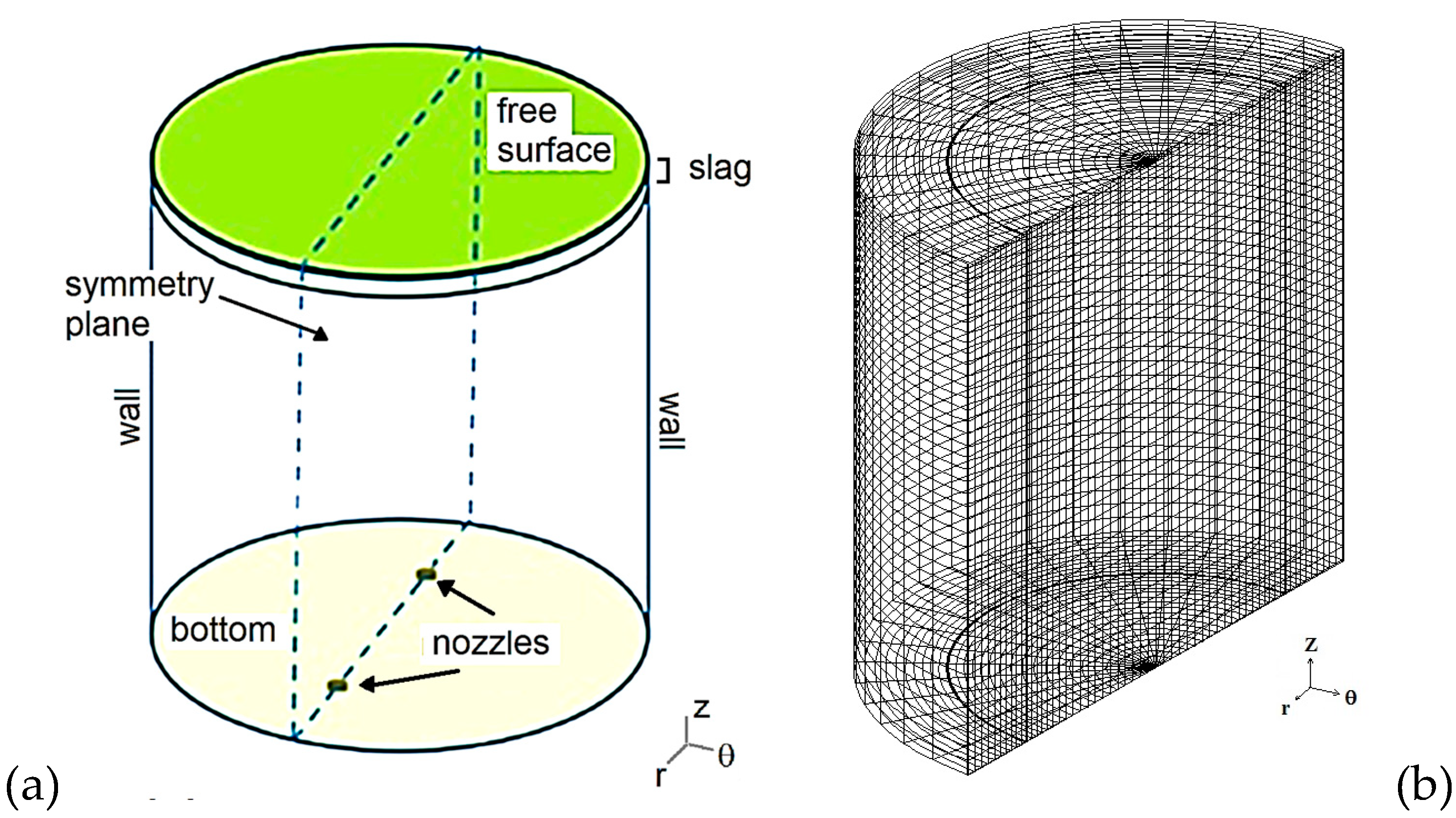
2.4. Initial and Boundary Conditions

2.4.1. Initial Conditions

Initially, all components of the velocity (u, v, w) for both phases are zero. Turbulence parameters are also zero for a static fluid. The entire domain is occupied by the two liquid phases (steel and a layer of slag above the steel) and no gas is originally present in the calculation (${\alpha }_l = 1, {\alpha }_l = 0)$. In the slag region; C₁ = 0 and C₃ = 1; in the steel region C₁ = 1 and C₃ = 0. Gas injection starts as the computation begins.

2.4.2. Boundary Conditions

The no-slip boundary condition is applied to the bottom and lateral walls of the ladle. This condition means that the components parallel and perpendicular to each wall are at zero speed so that all components of the liquid and gas phases are zero [6]. A standard wall function is applicable since the near-wall flows are not expected to be subjected to severe pressure gradients [6,32]. At the free surface zero axial gradients (or zero fluxes) of all variables are set except for the mass of gas, which is allowed to leave the system when bubbles reach the free surface. At the symmetry planes located at 0° and 180° in the azimuthal direction, as well as at the symmetry axis, all fluxes are zero. Finally, at the gas inlet (for single plug gas injection) or inlets (for dual plug gas injection), a mass flow rate of gas is set at the nozzle positions located at the bottom wall of the ladle.

Table 1. Boundary conditions of the mathematical model.

Variable/Boundary	Bottom Wall	Lateral Wall	Free Surface	Two Symmetry Planes (θ = 0° and θ = 180°)	Symmetry Axis at r = 0	Plug (Inlet or Inlets for both Single and Dual Gas Injection)
αg	$\frac{\partial {\alpha }_g}{\partial z}=0$	$\frac{\partial {\alpha }_g}{\partial r}=0$	$\frac{\partial {\alpha }_g}{\partial z}=0$	$\frac{\partial {\alpha }_g}{\partial \theta }=0$	$\frac{\partial {\alpha }_g}{\partial r}=0$	${\alpha }_g=1.0$
αl	$\frac{\partial {\alpha }_l}{\partial z}=0$	$\frac{\partial {\alpha }_l}{\partial r}=0$	$\frac{\partial {\alpha }_l}{\partial z}=0$	$\frac{\partial {\alpha }_l}{\partial \theta }=0$	$\frac{\partial {\alpha }_l}{\partial r}=0$	${\alpha }_l=0.0$
ug	$u_g=0.0$	$u_g=0.0$	$\frac{\partial u_g}{\partial z}=0$	$u_g=0.0$	$\frac{\partial u_g}{\partial r}=0$	$u_g=0.0$
vg	$v_g=0.0$	$v_g=0.0$	$\frac{\partial v_g}{\partial z}=0$	$\frac{\partial v_g}{\partial \theta }=0$	$v_g=0.0$	$v_g=0.0$
wg	$w_g=0.0$	$w_g=0.0$	$\frac{\partial w_g}{\partial z}=0$ But $w_g\ne 0.0$	$\frac{\partial w_g}{\partial \theta }=0$	$\frac{\partial v_g}{\partial r}=0$	$w_g=constant$ according to the gas flow rate and if the injection is single or dual
ul	$u_l=0.0$ standard wall functions	$u_l=0.0$ standard wall functions	$\frac{\partial u_l}{\partial z}=0$	$u_l=0.0$	$\frac{\partial u_l}{\partial r}=0$	$u_l=0.0$
vl	$v_l=0.0$ standard wall functions	$v_l=0.0$ standard wall functions	$\frac{\partial v_l}{\partial z}=0$	$\frac{\partial v_l}{\partial \theta }=0$	$v_l=0.0$	$v_l=0.0$
wl	$w_l=0.0$ standard wall functions	$w_l=0.0$ standard wall functions	$w_l=0.0$	$\frac{\partial w_l}{\partial \theta }=0$	$\frac{\partial w_l}{\partial r}=0$	$w_l=0.0$
k	k = 0.0	k = 0.0	$\frac{\partial k}{\partial z}=0$	$\frac{\partial k}{\partial \theta }=0$	$\frac{\partial k}{\partial r}=0$	k = 0.0
ε	ε = 0.0	ε = 0.0	$\frac{\partial \epsilon }{\partial z}=0$	$\frac{\partial \epsilon }{\partial \theta }=0$	$\frac{\partial k}{\partial r}=0$	ε = 0.0
C1	$\frac{\partial C_1}{\partial z}=0$	$\frac{\partial C_1}{\partial r}=0$	$\frac{\partial C_1}{\partial z}=0$	$\frac{\partial C_1}{\partial \theta }=0$	$\frac{\partial k}{\partial r}=0$	$C_1=0$
C3	$\frac{\partial C_3}{\partial z}=0$	$\frac{\partial C_3}{\partial r}=0$	$\frac{\partial C}{\partial z}=0$	$\frac{\partial C_3}{\partial \theta }=0$	$\frac{\partial k}{\partial r}=0$	$C_3=0$

gives a full description of the boundary conditions, based on the geometry shown in Figure 1a.

2.5. Solution Technique

The mathematical model was implemented in the CFD software PHOENICS (Version 2017, Concentration, Heat and Momentum Limited (CHAM), London, England). For validation purposes the experimental data from a scale water model were employed. Once the validation was completed, fluid flow phenomena in an industrial ladle furnace process was explored in more detail. The numerical solution involved the discretization of a 200 tons ladle into around 33,000 nodes in a polar cylindrical coordinate system with 22, 34 and 44 elements in angular radial and axial directions forming a non-uniform grid obtained after a thorough sensitivity analysis of the grid. A time step size of 0.5 s was used and convergence was achieved when imbalances of all conservation equations were below 1%. Figure 1b shows the grid of the ladle. As mentioned earlier, the commercial software PHOENICS used in this study is unable to couple IPSA and the VOF methods, due to inherent limitation of the solver. As such the VOF algorithm described in Section 2.2 was programmed through a separate subroutine, written in Fortran, and linked to the solver, in order to solve the marker equations associated to the VOF algorithm and then coupled to both the IPSA and VOF models.

3. Experimental Work

Ladle eye: A water-engine oil 1/17th physical model was employed to measure ladle eye. The geometric characteristics are listed in

Table 2. Geometrical and physical variables in the physical model.

Height of Liquid	Symbol	Value
Ladle
Diameter	D	0.21 m
Height of liquid	H	0.21 m
Nozzle
Diameter	D	0.005 m
Position	1/2 R for single injection
	2/3 R for dual injection
Air properties (room temperature)
Density	ρg	1.205 kg/m3
Viscosity	μg	1.74 × 10−5 kg/m·s
Bubble diameter	Dp	0.005 m
Gas flow rate	Q	13.8 × 10−5 m3/s
Water properties
Density	ρa	1000 kg/m3
Viscosity	μa	1 × 10−3 kg/m·s
Surface tension (water-air)	σ	728 mN/m
Engine oil properties
Density	ρe	800 kg/m3
Viscosity	μe	0.08 kg/m·s
Thickness	Δ	0.84 cm (4% in height)

. The ladle eye area was measured using a photographic technique. The area was computed using the image processing tools included in MATLAB. Formation of ladle eye is a highly dynamic process due to the discontinuous release of gas bubbles. Ladle eye was reported based on the average value of 15 photographs. Gas injection was carried out with one single nozzle located at 2/3 R. The oil thickness was constant equivalent to 4% of the height of water. The gas flow rate was 13.8 × 10⁻⁵ m³/s (8.3 NL min⁻¹).

Velocity patterns: Flow velocities and turbulent kinetic energy contours were obtained experimentally using particle image velocimetry (PIV, Dantec Dynamics, Denmark) with one single nozzle located at 2/3 R. PIV equipment was manufactured by Dantec Dynamics® and operated in the single frame with a time interval between pulses of 100 μs and using 30% of the total power of the laser of 10 mJ. Images were captured with a High Speed camera SpeedSense M320 (Skovlunde, Denmark) with a resolution of 1920 pixels × 1200 pixels. A total of 500 pair of photos were captured and statistically processed with the software DynamicStudio version 4.0 (Skovlunde, Denmark) to get the final results on flow patterns and turbulent intensity. Additional details can be found in [33].

4. Results

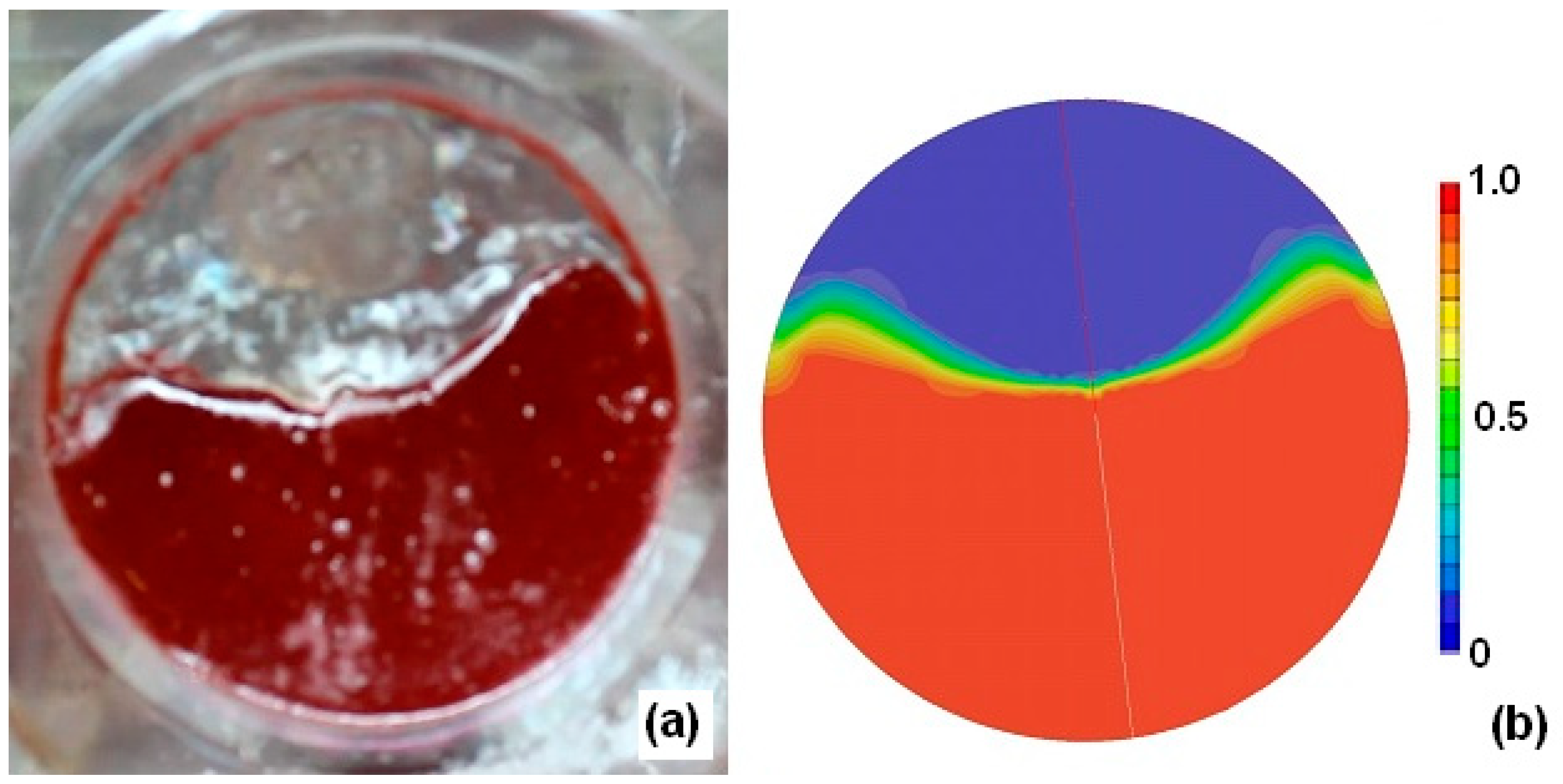
4.1. Model Validation

The mathematical model was validated using experimental data on ladle eye and velocity fields.

Figure 2 compares the slag eye area measured and that predicted by the model with a single plug gas injection. The experimental ladle eye was around 30%. The mathematical model also estimates a ladle eye area of around 30%. As seen, the agreement is quite good.

Figure 3 compares measured and computed turbulent kinetic energy contours in the longitudinal plane containing the nozzle for a single plug gas injection with a nozzle located 2/3 R and for a 1/17th physical model. Agreement is reasonably good since the maximum turbulent kinetic energy (k) is found in the plume and the order of magnitude is similar in both measured and computed contours as expected from the predictions and measurements. As seen in Figure 3, the mathematical model overestimates turbulence at the nozzle and at the free surface. The reason for the high values of k near the nozzle has been pointed out in Schwarz and Taylor [34]. Bubbles are formed at the nozzle, and the diameter of the bubbles is significantly larger than the nozzle. This means that the initial velocity of bubbles at the nozzle is comparatively smaller than the gas velocity through the nozzle. This deviation can be corrected using an “effective nozzle diameter”. This issue has been neglected in this study as at the nozzle, the gas holdup is very high so the local value of k computed does not seem to have any physical significance. At the free surface, the model does not allow the deformation of the free surface and therefore there is an overestimation that is explained by the flat free surface assumption. In spite of the deviation, it can be concluded that the mathematical model offers a good prediction of the experimental data with a maximum deviation of around 10% and if the over predicted zones of high k at the nozzle and at the free surface were eliminated, the predicted and measured k maps would have agreed much better. The Euler–Euler part of the model (IPSA) presented in this study has been extensively validated against experimental results of liquid velocity, gas holdup, and trace evolution in mixing experiments as indicated in [35]. The combination of the IPSA and VOF algorithms allowing the presence of two liquids is validated in this study through the slag eye area.

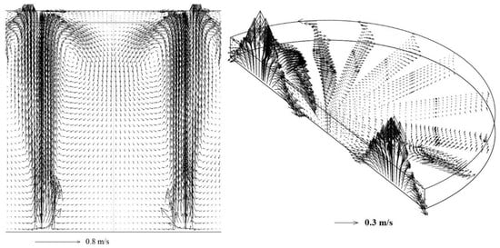
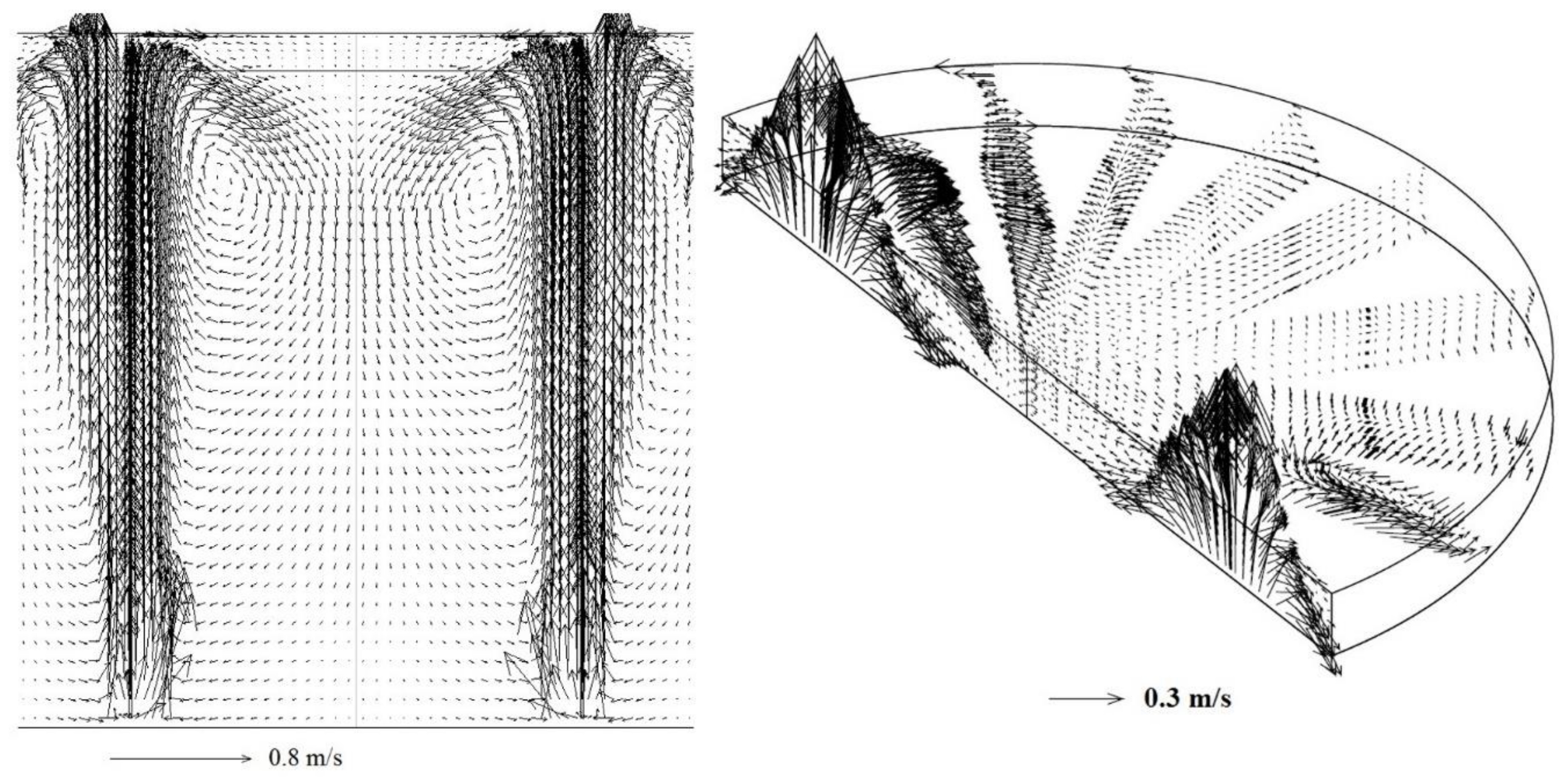
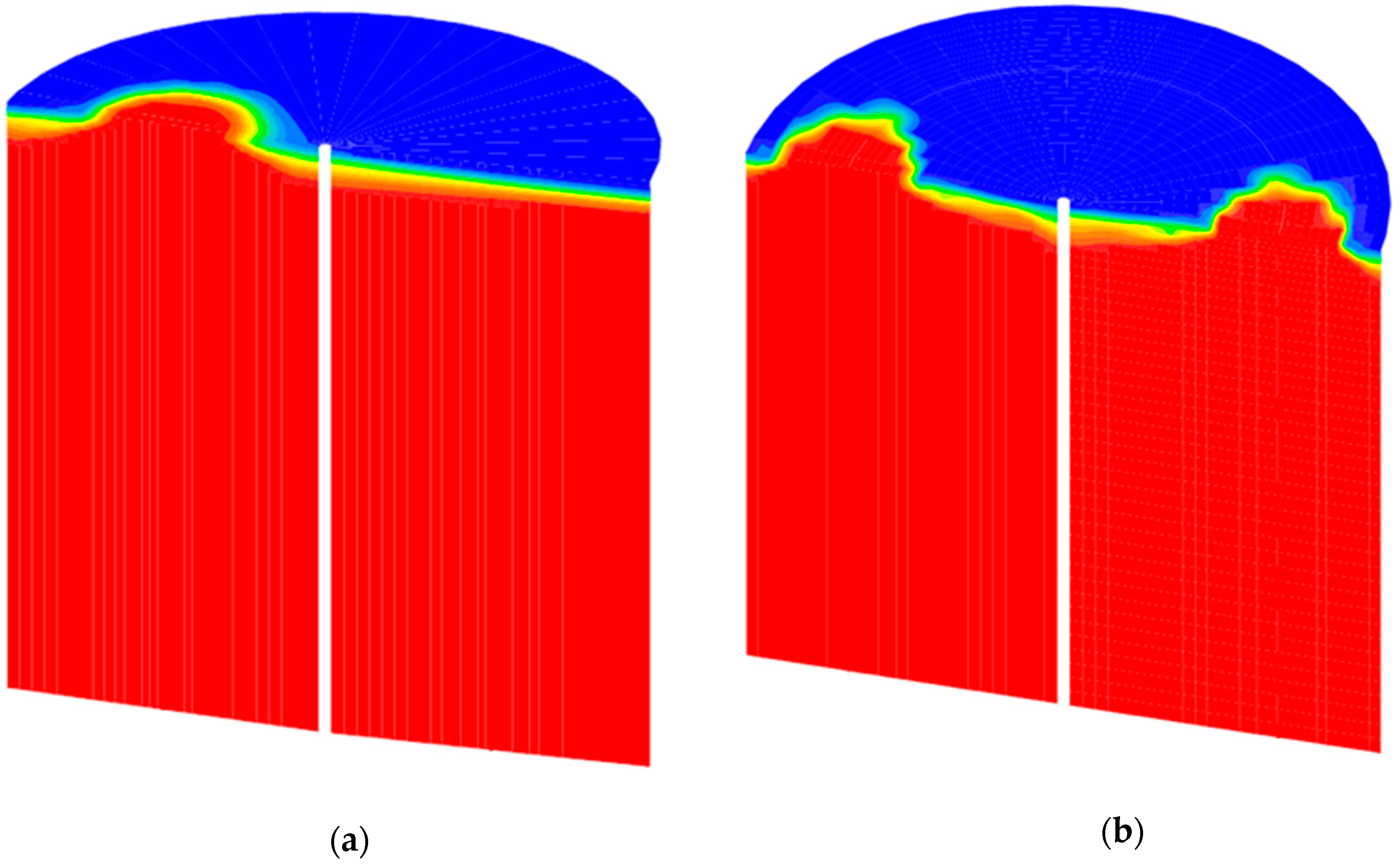
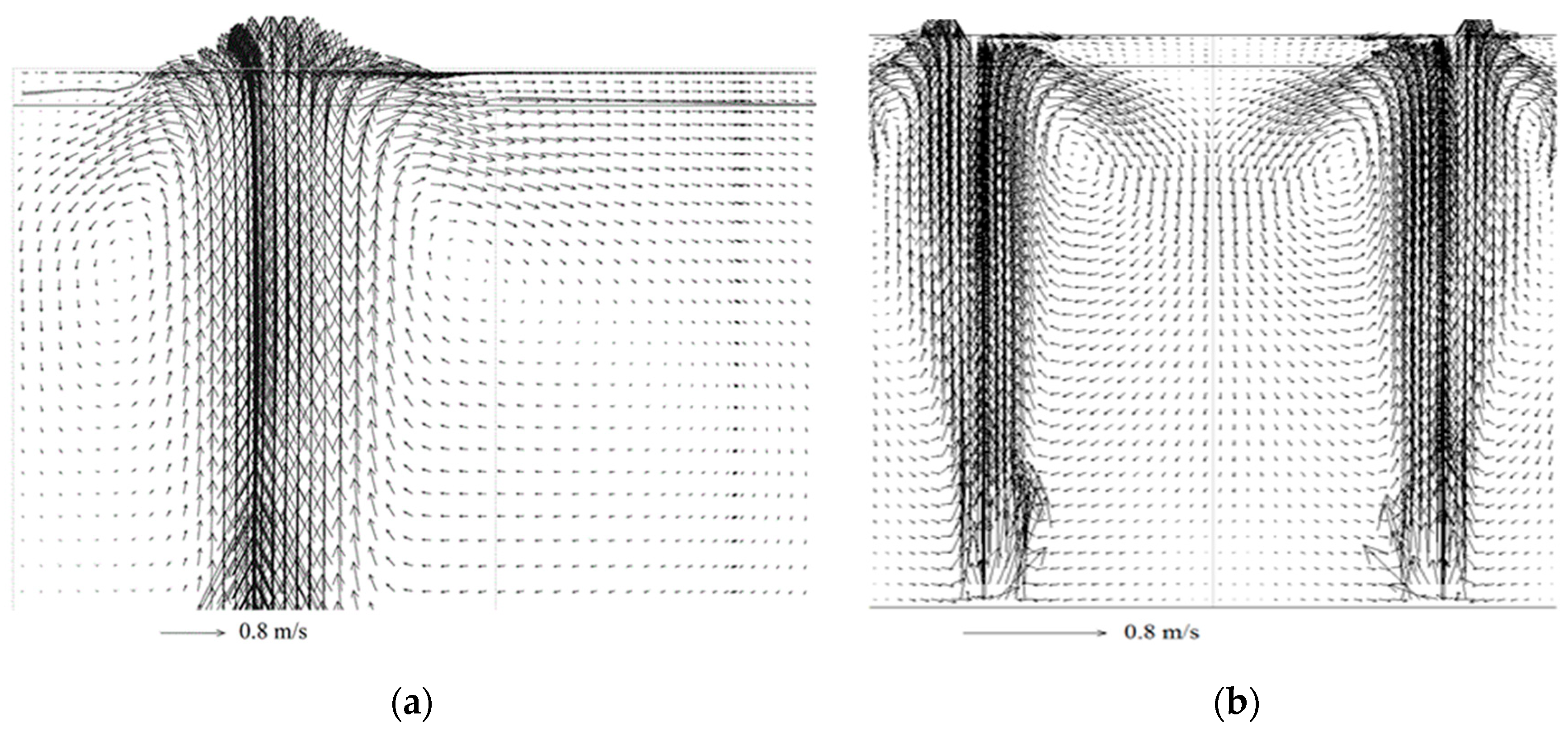
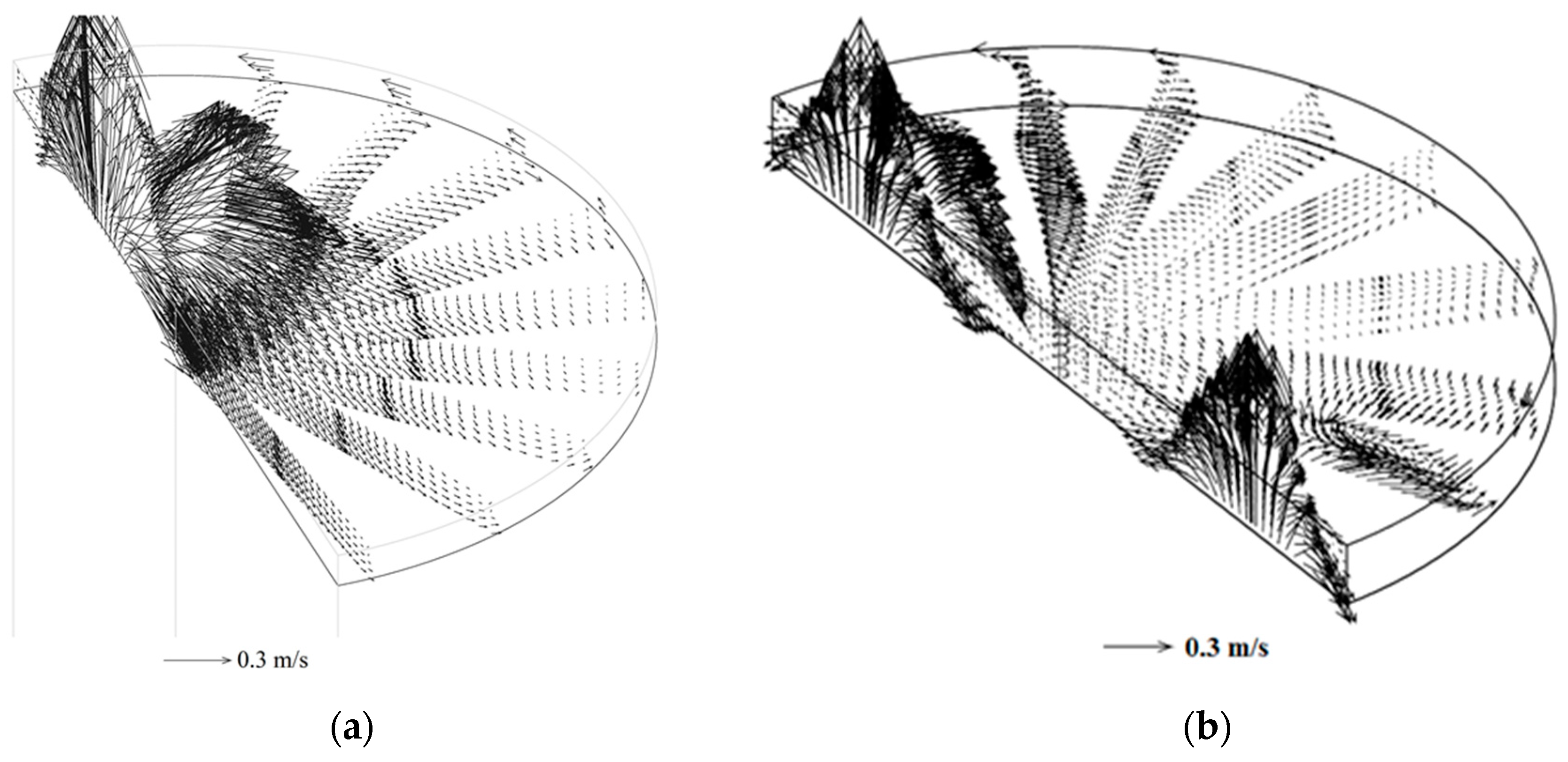
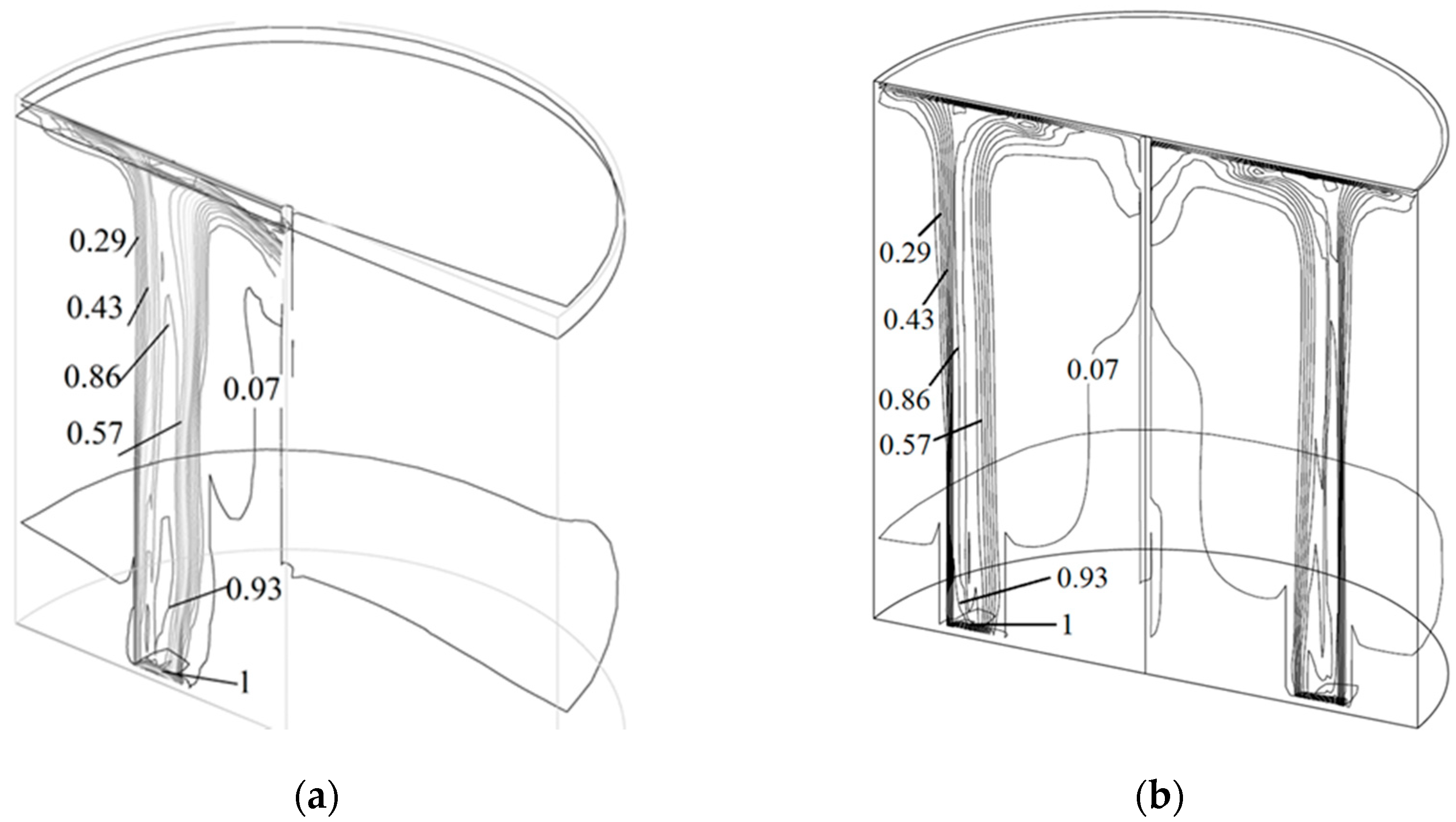
4.2. Flow Patterns of an Industrial Ladle

The mathematical model developed was applied to the industrial size ladle.

Table 3. Geometrical and physical variables needed for the simulations.

Parameter	Symbol	Value
Ladle
Diameter	D	3.58 m
Height	H	3.57 m
Nozzle
Diameter	D	0.013 m
Position	1/2 R, 2/3 R
Argon properties
Density	ρg	0.933 kg/m3
Viscosity	μg	2.2501 × 10−5 kg/m·s
Heat capacity	Cpg	520 J/kg K
Thermal conductivity	kg	0.01723 W/m·K
Bubble diameter	Dp	0.005 m
Gas flow rate	Q	9.72 × 10−3 m3/s
Argon temperature at inlet		311 K
Steel properties
Density	ρa	7200 kg/m3
Viscosity	μa	6.2 × 10−3 kg/m·s
Surface tension (argon-steel)	σ	1.8 N/m
Heat capacity	Cpa	789.9 J/kg·K
Thermal conductivity	ka	32.7 W/m·K
Emissivity	E	0.8
Initial Steel temperature	${\mathrm{T}}_{\mathrm{a}}^0$	1875 K
Slag properties
Density	ρe	2690 kg/m3
Viscosity	μe	0.266 kg/m·s
Heat capacity	Cpe	964.8 J/kg·K
Thermal conductivity	ke	1.5 W/m·K
Initial slag temperature	${\mathrm{T}}_{\mathrm{e}}^0$	1873 K
Slag layer	Δ	14.28 cm (4% thickness)

shows important physical and geometrical information of the 200 tons ladle from a steel plant in México used to run the calculations. The model was employed to get a full characterization of flow patterns, in terms of velocity fields, turbulence parameters and so on. Two simulations were performed. The first case includes one nozzle located at 2/3 R, a gas flow rate of 5.5 × 10⁻³ m³/s and a slag thickness of 4% H. The second simulation includes two nozzles located at 2/3 R, an angle of 180° between the nozzles, gas flow rates of 5.5 × 10⁻³ m³/s in each nozzle and the same slag thickness.

Figure 4 shows the two-liquid phase distribution in the ladle for both simulations. Only half of the ladle is shown due to symmetry. The two liquid phases are immiscible in each other and ideally a line should describe the interface. However, all mathematical models report some degree of error to represent an interface, called numerical diffusion. A finer grid around the interface, and higher-order convective schemes were used to mitigate the numerical diffusion. The results in this figure show that numerical diffusion is low, which is desired and is an indication of the accuracy of this model.

Figure 5a shows the liquid velocity fields for the single plug gas injection (i.e., one nozzle) case. The gas injected at the bottom forms bubbles that rise to the top surface. The two-phase region is called the plume. The motion of the bubbles drags liquid from the bottom to the top surface. On the top surface, gas escapes from the liquid opening the slag layer, forming the “slag eye”. Liquid molten steel collides with the top slag layer and is pushed backwards, forming a recirculation loop on each side of the plume. The position of the central part of each recirculation loop changes depending on the gas flow rate and slag thickness. Figure 6b shows the predicted velocity fields when two nozzles at 2/3 R are considered for the simulation. Here it can be seen that, due to the same effects explained above concerning the dragging of the liquid by the ascending currents of bubbles and to the collision of the liquid steel with the top slag layer, four recirculation loops are formed, each one on each side of the two plumes. Regarding the velocity fields in the slag layer, in Figure 5a it is observed in the case of one nozzle, that liquid steel flows away in opposite direction from the ascending plume when the top slag layer is reached and the slag appears to behave in a similar way flowing away from the spout to the opposite wall. Figure 5b shows a more complex velocity field in the slag layer when two nozzles are considered in the simulation, including the presence, in the slag layer region located between the plumes, of two recirculation loops.

Figure 6 shows more details of the velocity patterns in the slag layer. In Figure 6a, with single plug gas injection located at 1/2 R, it can be observed that when the slag flows away from the spout it reaches the reactor wall, turns to the left and follows through the peripheral region of the slag layer located near the wall, returning to the spout region. Figure 6b, with dual plug gas injection, shows the prediction of more complex flow patterns in the slag layer due to the interactions of the slag currents leaving each one of the two plumes regions and colliding with each other in the symmetry axis zone, and colliding with the reactor walls.

Figure 7 shows the volume gas fraction in the plumes or gas hold up for the two cases taken as examples of the model output (single gas injection with a nozzle at 1/2 R and dual injection with nozzles located at 2/3 R). The plume region is clearly determined from these plots, which forms a plume in the shape of a cylinder that shows a lateral dispersion at the free surface. The shape and size of the plume is an important parameter to estimate the degree of mixing of liquid steel. As the diameter of this plume increases, it is expected to get higher mixing as noted by Conejo et al. [36]. It is noticed that the gas fraction is higher in the central axis of each plume. This is because there are no diffusion barriers for the gas phase it would be expected a lower gas concentration in the central plume when the free surface is reached. The high value of gas hold up in this figure requires further analysis. Figure 8; Figure 9 shows characteristic slip velocities and the forces dominating the flow dynamics such as the ratio of inertial over viscous forces (Reynolds number) and inertial over surface tension forces (Weber number) in the plume regions for both simulations (single and dual plug gas injections) with the aim of providing with further description of the fluid flow behavior of the ladle. Weber numbers are below 10 with both the injections, while average Reynolds numbers are around 1500 and relative velocities of around 0.15 m/s are found in this regions.

The results depicted in Figure 8 and Figure 9 suggest that the numerical procedure proposed in this study is able to provide detailed information on the dominating forces and relative motion of the phases.

5. Conclusions

A comprehensive mathematical model has been developed with an improved methodology to study multiphase flow applying two algorithms, IPSA and VOF using the CFD code PHOENICS. This unconventional approach to represent a two-immiscible liquid phase system stirred by gas injection through single and dual plugs located at the bottom of the ladle was developed by a hybrid combination of a Eulerian representation of a two–phase (dispersed gas bubbles into a continuous single liquid) and a VOF method to separate the liquid into two immiscible liquids (steel and slag). A comparison of experimental data (both centric and off-centric) from a 1/17th water-oil stirred ladle model, involving the values of slag eye area and turbulent kinetic energy, show a reasonable agreement and it is considered that the model has been successfully validated. The application of the developed model in an industrial size ladle indicates the potential to reach a full representation of the flow structure in both liquids, steel and slag. The model provides information on the geometry of the plume, velocity fields and turbulence parameters.

References

1. Mazumdar, D.; Guthrie, R.I.L. The Physical and Mathematical Modelling of Gas Stirred Ladle Systems. ISIJ Int. 1995, 35, 1–20. [Google Scholar] [CrossRef]
2. Liu, Y.; Ersson, M.; Liu, H.; Jönsson, P.G.; Gan, Y. A review of physical and numerical approaches for the study of gas stirring in ladle metallurgy. Metall. Matls. Trans. B 2019, 501, 555–577. [Google Scholar] [CrossRef]
3. Joo, V.; Guthrie, R.I.L. Modeling flows and mixing in steelmaking ladles designed for single- and dual-plug bubbling operations. Met. Trans. B 1992, 23, 765–778. [Google Scholar] [CrossRef]
4. Goldschmit, M.B.; Owen, A.H.C. Numerical modelling of gas stirred ladles. Ironmak. Steelmak. 2001, 28, 337–341. [Google Scholar] [CrossRef]
5. Markatos, N.C. The mathematical modelling of turbulent flows. Appl. Math. Model. 1986, 10, 190–220. [Google Scholar] [CrossRef]
6. Launder, B.E.; Spalding, D.B. The numerical computation of turbulent flows. Comput. Methods Appl. Mech. Eng. 1974, 3, 269–289. [Google Scholar] [CrossRef]
7. Mazumdar, D.; Guthrie, R.I.L. A comparison of three mathematical modeling procedures for simulating fluid flow phenomena in bubble-stirred ladles. Metall. Mater. Trans. B 1994, 251, 308–312. [Google Scholar] [CrossRef]
8. Mazumdar, D.; Guthrie, R.I.L. On mathematical models and numerical solutions of gas stirred ladle systems. Appl. Math. Model. 1993, 17, 255–262. [Google Scholar] [CrossRef]
9. Sheng, Y.Y.; Irons, G.A. Measurement and modeling of turbulence in the gas/liquid two-phase zone during gas injection. Metall. Mater. Trans. B 1993, 24, 695–705. [Google Scholar] [CrossRef]
10. Sichen, D. Modeling Related to Secondary Steel Making. Steel Res. Int. 2012, 83, 825–841. [Google Scholar] [CrossRef]
11. Jonsson, L.; Jönsson, P. Modeling of Fluid Flow Conditions around the Slag/Metal Interface in a Gas-stirred Ladle. ISIJ Int. 1996, 36, 1127–1134. [Google Scholar] [CrossRef]
12. Méndez, C.G.; Nigro, N.; Cardona, A.; Begnis, S.S.; Chiapparoli, W.P. Physical and Numerical Modelling of a Gas Stirred Ladle. Mecánica Computacional 2002, 21, 2646–2654. [Google Scholar]
13. Han, J.W.; Heo, S.W.; Kam, D.H.; You, B.D.; Pak, J.J.; Song, H.S. Transient Fluid Flow Phenomena in a Gas Stirred Liquid Bath with Top Oil Layer—Approach by Numerical Simulation and Water Model Experiments. ISIJ Int. 2001, 41, 1165–1172. [Google Scholar] [CrossRef] [Green Version]
14. Olsen, J.E.; Cloete, S. Coupled DPM and VOF model for analyses of gas stirred ladles at higher gas rates. In Proceedings of the 7th International Conference on CFD in the Minerals and Process Industries, CSIRO, Melbourne, Australia, 9–11 December 2009; pp. 1–6. [Google Scholar]
15. Hoang, Q.N.; Ramírez-Argáez, M.A.; Conejo, A.N.; Blanpain, B.; Dutta, A. Numerical Modeling of Liquid-Liquid Mass Transfer and the Influence of Mixing in Gas-Stirred Ladles. J. Met. 2018, 70, 2109–2118. [Google Scholar] [CrossRef]
16. Li, B.; Yin, H.; Zhou, C.-Q.; Tsukihashi, F. Modeling of three-phase flows and behavior of slag/steel interface in an argon gas stirred ladle. ISIJ Int. 2008, 48, 1704–1711. [Google Scholar] [CrossRef]
17. Sulasalmi, P.; Visuri, V.V.; Kärnä, A.; Fabritius, T. Simulation of the Effect of Steel Flow Velocity on Slag Droplet Distribution and Interfacial Area Between Steel and Slag. Steel Res. Int. 2015, 86, 212–222. [Google Scholar] [CrossRef]
18. Huang, A.; Harmuth, H.; Doletschek, M.; Vollmann, S.; Feng, X. Toward CFD Modeling of Slag Entrainment in Gas Stirred Ladles. Steel Res. Int. 2015, 86, 1447–1454. [Google Scholar] [CrossRef]
19. Li, L.; Liu, Z.; Li, B.; Matsuura, H.; Tsukihashi, F. Water Model and CFD-PBM Coupled Model of Gas-Liquid-Slag Three-Phase Flow in Ladle Metallurgy. ISIJ Int. 2015, 55, 1337–1346. [Google Scholar] [CrossRef] [Green Version]
20. Singh, U.; Anapagaddi, R.; Mangal, S.; Padmanabhan, K.A.; Singh, A.K. Multiphase Modeling of Bottom-Stirred Ladle for Prediction of Slag–Steel Interface and Estimation of Desulfurization Behavior. Metall. Mater. Trans. B 2016, 47, 1804–1816. [Google Scholar] [CrossRef]
21. Haiyan, T.; Xiaochen, G.; Guanghui, W.; Yong, W. Effect of Gas Blown Modes on Mixing Phenomena in a Bottom Stirring Ladle with Dual Plugs. ISIJ Int. 2016, 56, 2161–2170. [Google Scholar] [CrossRef] [Green Version]
22. Hirt, C.W.; Nichols, B.D. Volume of fluid (VOF) method for the dynamics of free boundaries. J. Comput. Phys. 1981, 39, 201–225. [Google Scholar] [CrossRef]
23. Spalding, D.B. IPSA 1981: New Developments and Computed Results; Imperial College, CFDU Report HTS/81/2; Concentration, Heat & Momentum Limited: London, UK.
24. Schwarz, M.P. Simulation of gas injection into liquid melts. Appl. Math. Model. 1996, 20, 41–51. [Google Scholar] [CrossRef] [Green Version]
25. Davis, M.P.; Pericleous, K.; Cross, M.; Schwarz, M.P. Mathematical Modelling Tools for the Optimization of Direct Smelting Processes. Appl. Math. Model. 1998, 22, 921–940. [Google Scholar] [CrossRef]
26. Stephens, D.; Tabib, M.; Davis, M.; Schwarz, M.P. CFD Simulation of bath dynamics in the HIsmelt smelt reduction vessel for iron production. Prog. Comput. Fluid Dyn. 2012, 12, 196–206. [Google Scholar] [CrossRef]
27. Davidson, J.F.; Harrison, D. Fluidized Particles; Cambridge University Press: London, UK; New York, NY, USA, 1963. [Google Scholar]
28. Kuo, J.T.; Wallis, G.B. Flow of bubbles through nozzles. Int. J. Multiphase Flow 1998, 14, 547–564. [Google Scholar] [CrossRef]
29. Lopez de Bertodano, M. Turbulent Bubbly Flow in a Triangular Duct. Ph.D. Thesis, Rensselaer Polytechnic Institute, Troy, NY, USA, 1991. [Google Scholar]
30. Ramshaw, J.D.; Trapp, J.A. A numerical technique for low-speed homogeneous two-phase flow with sharp interfaces. J. Comput. Phys. 1976, 21, 438–453. [Google Scholar] [CrossRef]
31. Roe, P.L. Characteristic-Based Schemes for the Euler Equations. Ann. Rev. Fluid Mech. 1986, 18, 337–365. [Google Scholar] [CrossRef]
32. El Gharbi, N.; Absi, R.; Benzaoui, A.; Amara, E.H. Effect of near-wall treatments on airflow simulations. In Proceedings of the International Conference on Computational Methods for Energy Engineering and Environment: ICCM3E, Sousse, Tunisia, 20–22 November 2009; pp. 185–189. [Google Scholar]
33. Ramírez-Argáez, M.; González-Rivera, C. Modeling of Metal-Slag Mass and Momentum Exchanges in Gas-Stirred Ladles. In Proceedings of the 3rd Pan American Materials Congress; Springer: Berlin/Heidelberg, Germany, 2017; pp. 771–781. [Google Scholar]
34. Schwarz, M.P.; Taylor, I.F. CFD and Physical Modelling of Slag-Metal Contacting in a Smelter. In Proceedings of the 4th World Conference on Applied Fluid Mechanics, Freiburg, Germany, 7–11 June 1998; Volume 4, pp. 1–15. [Google Scholar]
35. Ramírez-Argáez, M.A. Mathematical Modeling of DC Electric Arc Furnace Operations. Ph.D. Thesis, MIT, Cambridge, MA, USA, 2000; pp. 165–174. [Google Scholar]
36. Conejo, A.; Kitamura, S.; Maruoka, N.; Kim, S. Effects of Top Layer, Nozzle Arrangement, and Gas Flow Rate on Mixing Time in Agitated Ladles by Bottom Gas Injection. Metall. Mater. Trans. B 2013, 44, 914–923. [Google Scholar] [CrossRef]
Figure 1. (a) Schematic view of the gas stirred ladle with nozzle (both single and dual plug gas injections), (b) Cylindrical grid coordinates of the ladle (axisymmetric section) used in the simulations.
Processes 07 00175 g001
Figure 2. (a) Physical model with a scale factor of 1/17th to observe steel–slag behavior using water–engine oil respectively (b) Calculated ladle eye with mathematical model.
Processes 07 00175 g002
Figure 3. Model validation using turbulent kinetic energy data obtained by (a) particle image velocimetry (PIV) and (b) numerical simulation. The computational fluid dynamics (CFD) model results show a good prediction of experimental results.
Processes 07 00175 g003
Figure 4. Steel–slag distribution (Steel, red phase; blue, slag phase) according to the mathematical model predictions considering the two cases in this study (a) single plug gas injection with nozzle at 1/3 R and (b) dual plug gas injection with nozzles at 2/3 R, observing a small numerical diffusion due to the use of a finer grid in the said interface, improving the degree of precision.
Processes 07 00175 g004
Figure 5. Velocity fields are shown in the plane of symmetry of the ladle furnace (a) single plug gas injection, the liquid metal shows two recirculation on the sides of the single nozzle, generated by the drag of the bubbles on the liquid steel, (b) dual plug gas injection creates two plumes with two circulating loops on each side of each plume. The flow patterns in the slag layer are different for both injections (single or dual).
Processes 07 00175 g005
Figure 6. Details of 3D velocity patterns on the top slag layer (a) Single plug gas injection (i.e., one nozzle) located at 1/2 R; (b) dual plug as injection (two nozzles) located at 2/3 R. In both the cases, a complex slag flow pattern is observed.
Processes 07 00175 g006
Figure 7. Gas plume that forms in the mathematical simulation of the ladle furnace adopted a cylindrical shape and shows a greater fraction of gas in the central axis of the plume and has a single plume for (a) single plug gas injection and two plumes for (b) dual plug gas injection.
Processes 07 00175 g007
Figure 8. Single plug gas injection (one nozzle) simulation: Gas-bubble characteristics in the system: (a) Weber number, (b) Reynolds number and (c) Slip velocity in m/s.
Processes 07 00175 g008
Figure 9. Dual plug gas injection (two nozzles) simulation: Gas-bubble characteristics in the system: (a) Weber number, (b) Reynolds number and (c) Slip velocity in m/s.
Processes 07 00175 g009