Energy-Efficient Train Driving Strategy with Considering the Steep Downhill Segment


Abstract
:1. Introduction
- Considering the route with a steep downhill, the solution space for a given cruising speed is analyzed to obtain the classical energy-efficient driving strategy for a given trip time.
- A local optimization approach is developed to reduce the traction energy consumption for trains running in the steep downhill segment by applying the dichotomization algorithm.
- A global optimization is achieved with the utilization of the adaptive gradient descent method to calculate the optimal cruising speed, which corresponds to the minimum traction energy consumption.
2. Problem Description
2.1. Assumptions
- The train is considered as a mass point when running on the track, and its mass is fixed.
- The slope of the centroid of the train represents the gradient of the entire vehicle.
- The traction efficiency is assumed to be constant, and the mechanical energy is used as the traction energy during the trip.
- The regenerative braking is not considered in the train model, because we only consider optimizing the driving strategy of a single train in this work.
2.2. Model Formulation
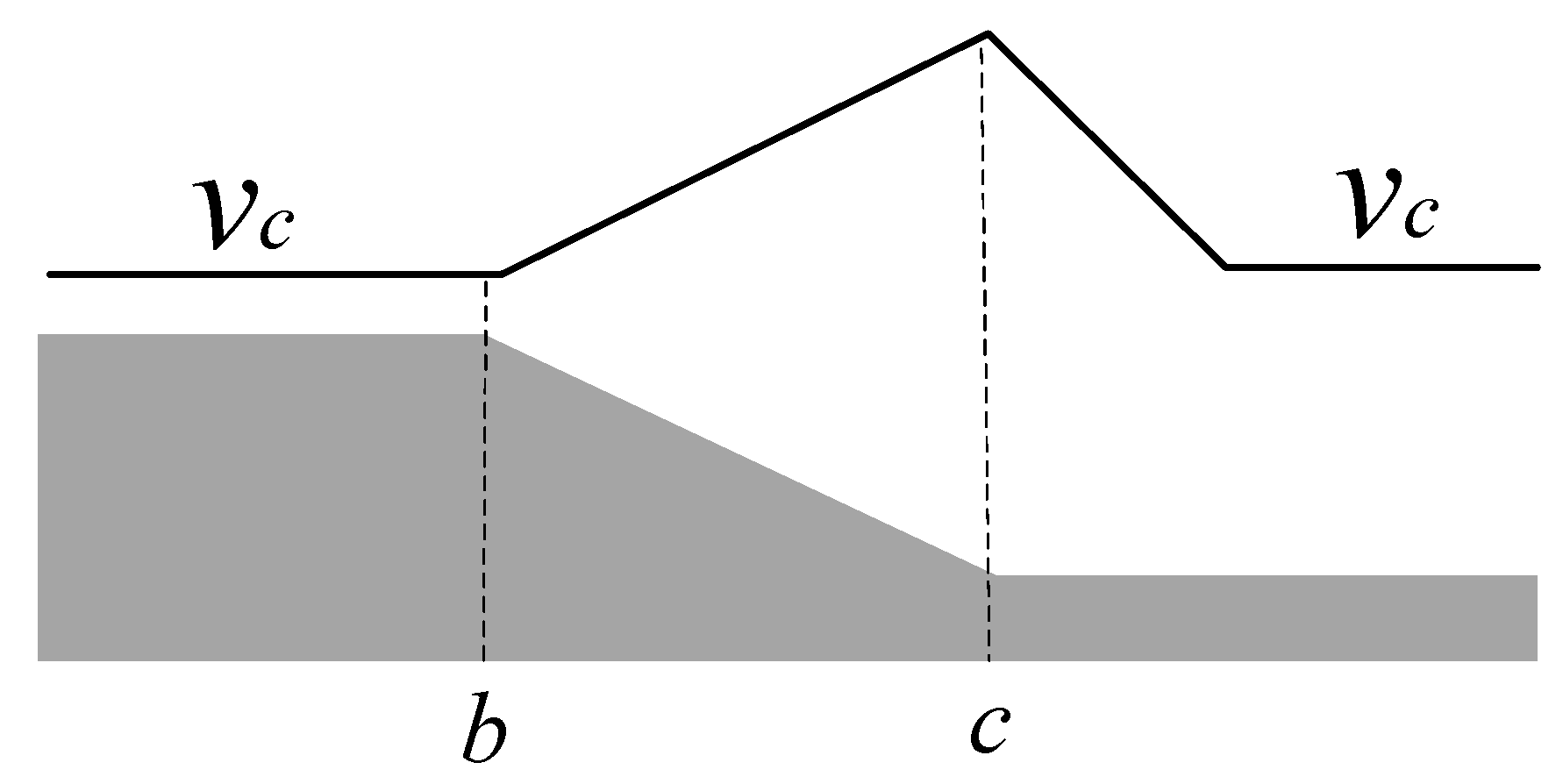
2.3. Definition of Steep Downhill
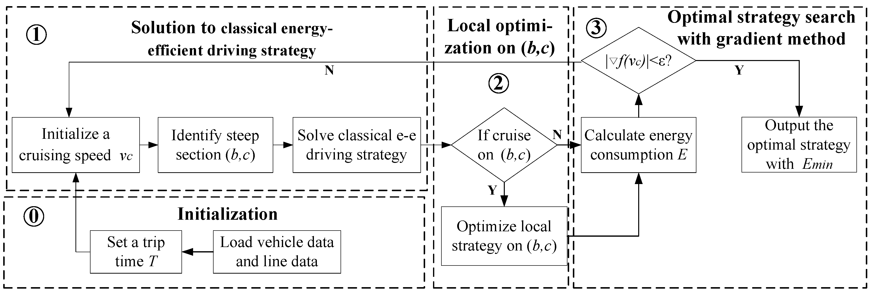
3. Solution Approach
- Initialization: Load line data and vehicle data and set a planned trip time T.
- Solution to classical energy-efficient driving strategy: Initialize a cruising speed , identify steep segment and solve classical energy-efficient driving strategy.
- Local optimization on : Judge the driving regime of the train in the steep downhill; if the train is cruising in this segment, then optimize the local driving strategy of the segment.
- Optimal strategy search with adaptive gradient method: Calculate energy consumption and use the gradient method to solve the cruising speed corresponding to the minimum traction energy consumption, and then obtain the optimal energy-efficient driving strategy.
3.1. Calculation of Classical Energy-Efficient Driving Strategy
3.1.1. Analysis of Energy-Efficient Driving Regimes
- : should be 1 and is 0, which implies the Maximum traction regime.
- : should be 0 and may vary in (0,1), which indicates the Partial traction phase; : should be 0, and may vary in (0,1), which suggests the Partial braking phase. These two phases only exist for the Cruising regime by analyzing Equation (11).
- : should be 1 and is 0, which implies the Maximum braking regime.
- : Both and should be 0, which suggests the Coasting regime.
3.1.2. Solution Space Analysis
- denotes the trip time of the driving strategy that the train begins to coast as soon as it reaches the cruising speed at the position .
- denotes the trip time of the driving strategy that the train begins to coast at the initial position of the steep slope.
- denotes the trip time of the driving strategy that the train begins to coast at the final position of the steep slope.
- denotes the trip time of the driving strategy that the train begins to coast at the position when the train speed reaches the braking profile.
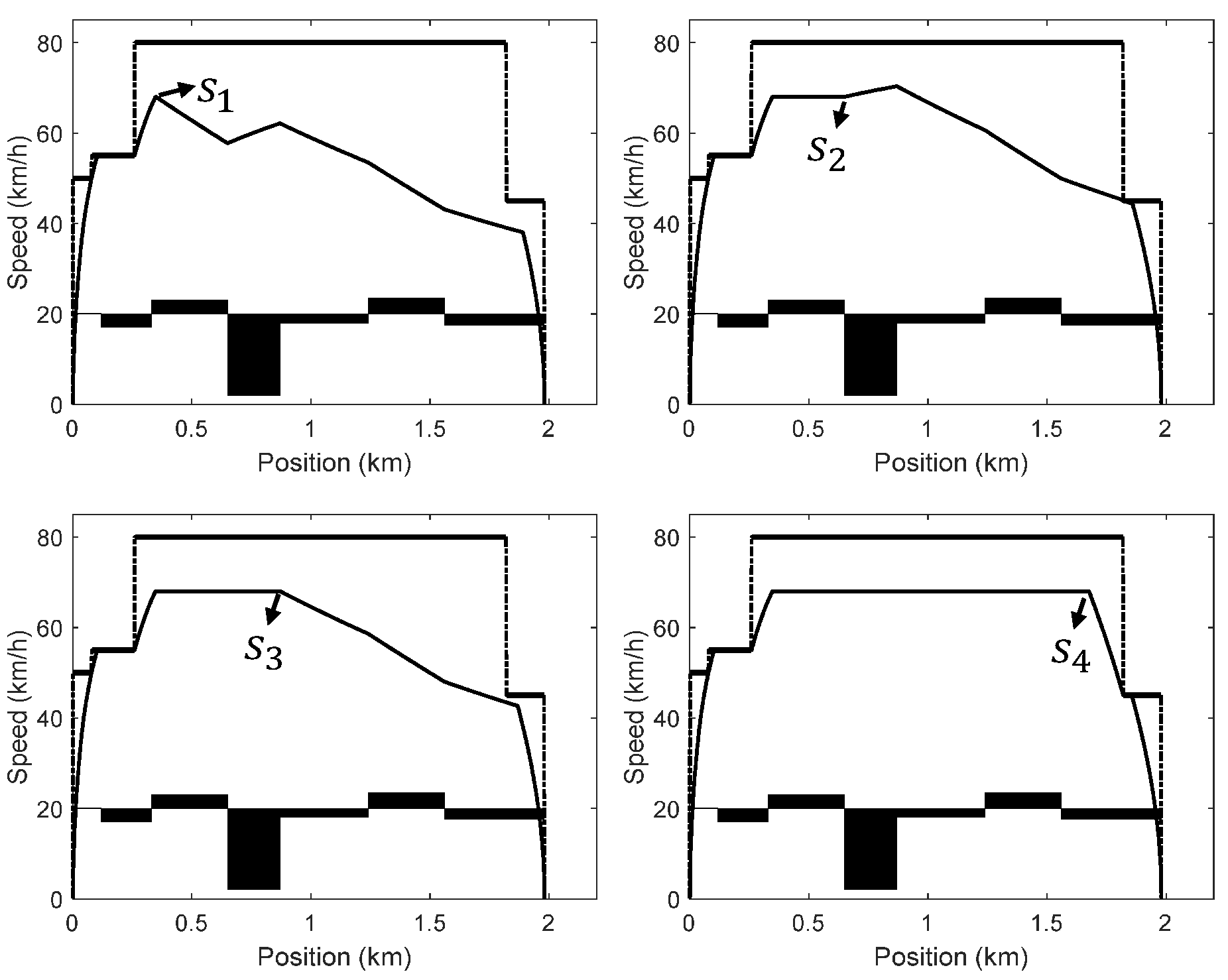
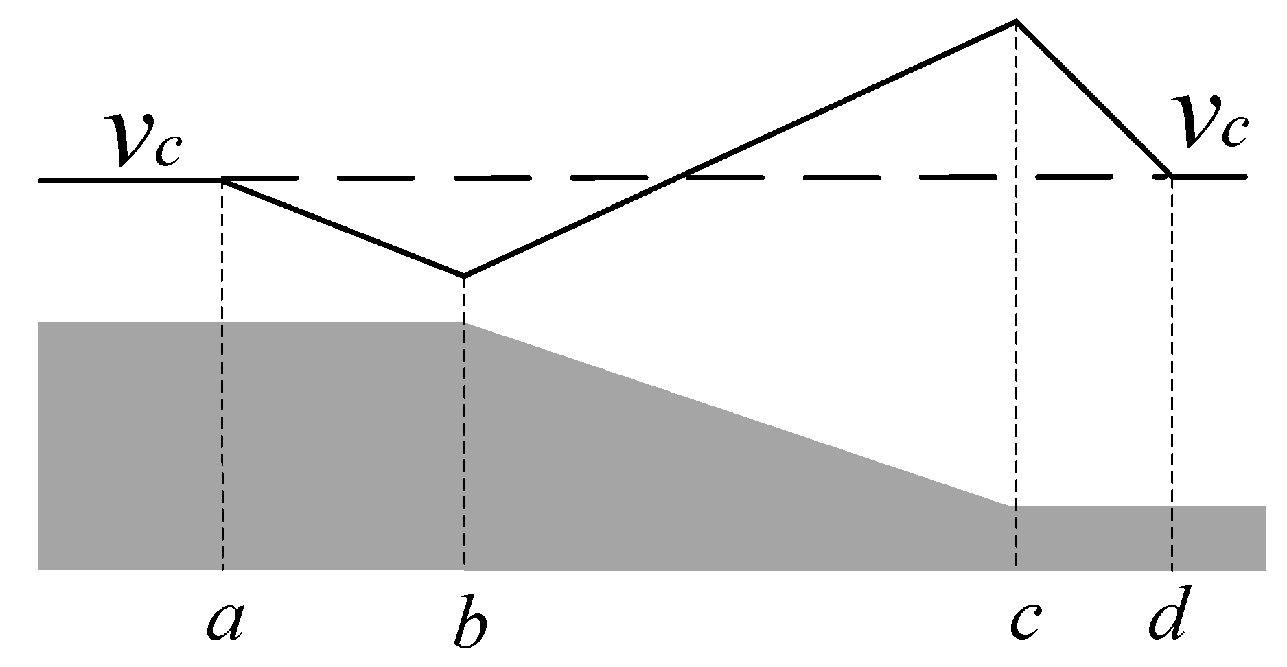
- Scenario 1: (Figure 5a). This situation always happens for the scenario that the steep downhill is relatively short and exists in the middle of the line. For the segment , when the train begins to coast later, the trip time with a higher average coasting speed will be shorter, i.e., . Coasting from the position makes the train speed increase due to the steep slope such that the speed in the steep slope and the following segment is higher, which indicates . In addition, a small steep slope has a small effect on the average train speed. Keeping the cruising speed on the segment can achieve a short trip time, i.e., . The train speed will decrease without traction and steep slopes after . Hence, we have . In conclusion, , , and will satisfy .
- Scenario 2: (Figure 5b). This situation generally happens for the scenario that the steep downhill exists in the second half of the line. Differing from the first situation, due to the steep slope exists in the second half, coasting from the position makes the average train speed higher than the cruising speed in the segment , i.e., . As a result, , , and will satisfy .
- Scenario 3: (Figure 5c). This situation always happens when the steep downhill is relatively short and exists in the first half of the line. After accelerating to the cruising speed, the train immediately enters the steep downhill segment, and the speed rises to exceed the cruising speed such that the average running speed of the train in the segment is greater than the cruising speed, i.e., . Thus, , , and will satisfy .
- Scenario 4: (Figure 5d). This situation exists when the steep downhill is relatively long and exists in the first half of the line. Because a longer steep slope has a greater effect on the average train speed, coasting from the position makes the average train speed higher than the cruising speed for the segment , i.e., . Therefore, , , and will satisfy .
- Scenario 5: (Figure 5e). This situation happens when the relatively long steep downhill exists in the first half of the line, and there is a downward slope, but not a steep downhill, in the segment . Compared with Scenario 4, a downward slope in the segment brings a higher initial speed before stepping into the steep downhill, hence, the average train speed will be higher than the cruising speed in the segment , that is, the trip time will be shorter (). Consequently, , , and will satisfy .
3.1.3. Coasting Position Calculation
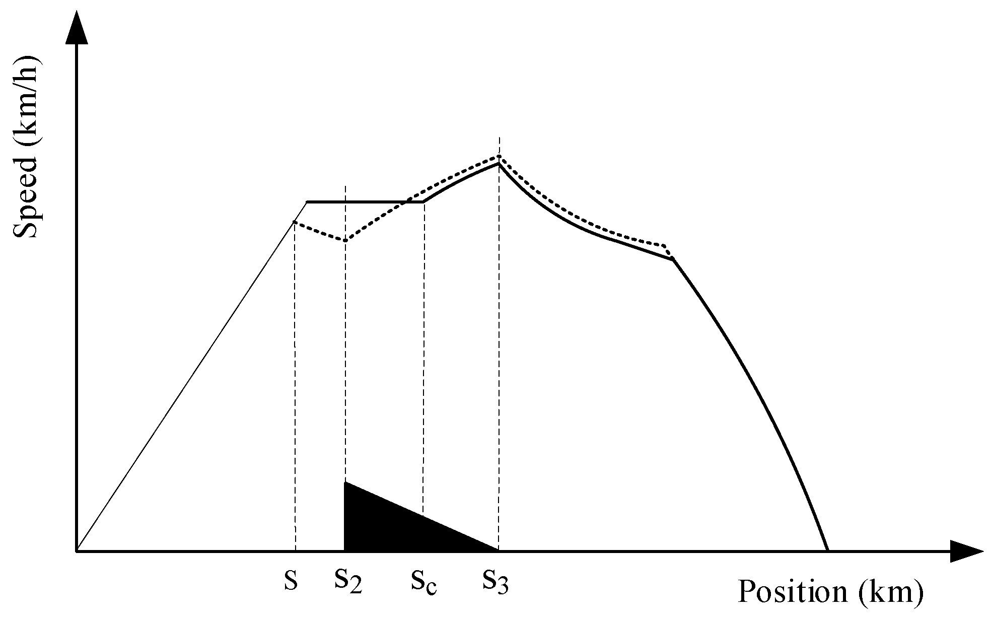
- or : In Figure 5a, the horizontal line from the ordinate T intersects the curve in the figure at a unique point or , which indicates the optimal coasting position with the trip time T exists in the segment or , and the solution is unique in these two situations.
- : There will be three solutions, which belong to , and , respectively. Due to the principle that, when the running times are the same, a longer coasting distance contributes to a smaller traction energy consumption, the optimal coasting position should be found in .
3.2. Local Optimization on Steep Downhill Segment
| Algorithm 1: The dichotomization algorithm for calculating the optimal coasting position. |
| Step 1. Give a search segment ( initially setting and ) and an error , and verify |
| ; |
| Step 2. Calculate the midpoint of the segment and its time function ; |
| Step 3. If , then turn to step (4); otherwise, turn to step (5); |
| Step 4. If , then output the coasting point ; otherwise, return to step (2) with setting |
| ; |
| Step 5. If , then output the coasting point ; otherwise, return to step (2) with setting |
| . |
3.3. Calculation of the Optimal Cruising Speed With Adaptive Gradient Descent Method
| Algorithm 2: The ADG algorithm for calculating the optimal cruising speed. |
| Step 1. Give a cruising speed set the allowable error , the number of iterations and initialize a step size parameter ; |
| Step 2. Calculate the traction energy consumption and the gradient with ; |
| Step 3. Take the negative gradient direction as the search direction and determine the step size by |
| Step 4. Search the next cruising speed and calculate and |
| Step 5. Determine whether the termination condition is satisfied. If yes, then output the optimal strategy with . Otherwise, set , and return to step (2). |
4. Simulation Results
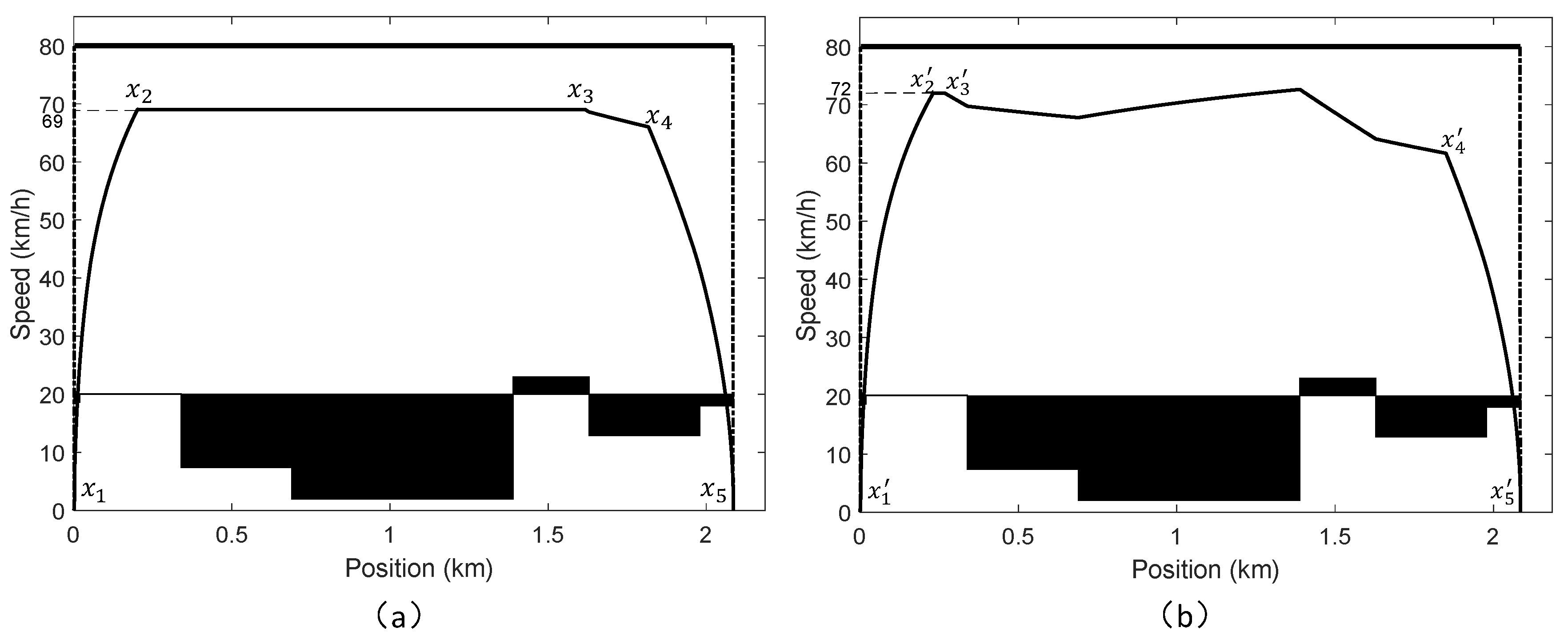
4.1. Case 1
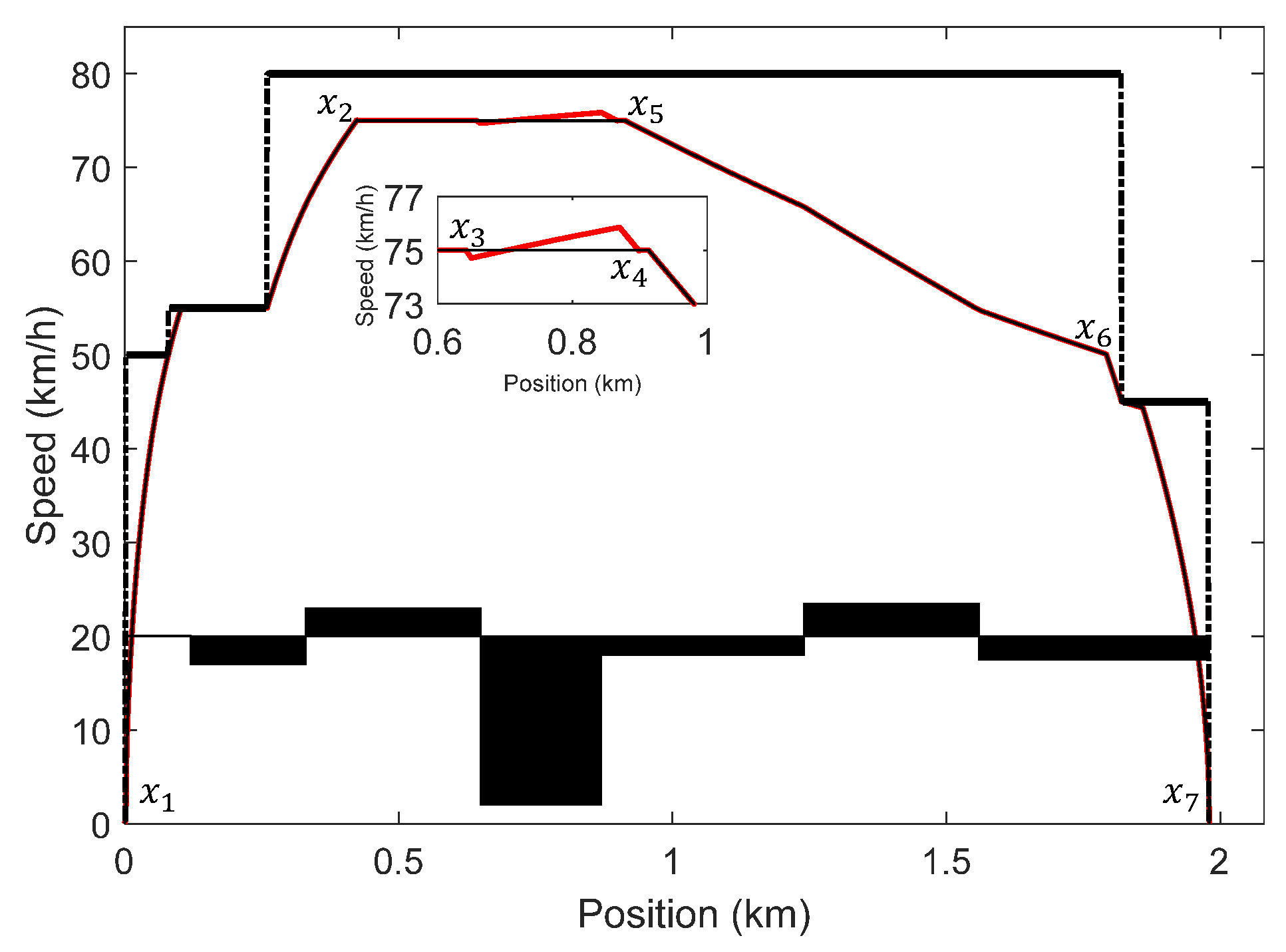
4.2. Case 2
5. Conclusions
Author Contributions
Funding
Conflicts of Interest
References
- Su, S.; Tang, T.; Li, X.; Gao, Z.Y. Optimization on multi-train operation in subway system. IEEE Trans. Intell. Transp. 2014, 15, 673–684. [Google Scholar]
- Liu, W.T.; Tang, T.; Su, S.; Chang, Y.H.; Li, X.L. Study on the energy-efficient driving strategy for trains running in the steep downhill section. In Proceedings of the International Conference on Electronic, Control Automation and Mechanical Engineering, Sanya, China, 19–20 November 2017; pp. 534–539. [Google Scholar]
- Milroy, I.P. Aspects of Automatic Train Control. Ph.D. Thesis, Loughborough University, Loughborough, UK, 1980. [Google Scholar]
- Asnis, I.; Dmitruk, A.; Osmolovskii, N. Control of the motion of a train by the maximum principle. Energy Optim. USSR Comput. Math. Math. Phys. 1985, 25, 37–44. [Google Scholar] [CrossRef]
- Howlett, P.G. An optimal strategy for the control of a train. J. Aust. Math. Soc. B 1990, 31, 454–471. [Google Scholar] [CrossRef]
- Howlett, P.G.; Milroy, I.P.; Pudney, P.J. Energy-efficient train control. Control Eng. Pract. 1994, 2, 193–200. [Google Scholar] [CrossRef]
- Khmelnitsky, E. On an optimal control problem of train operation. IEEE Trans. Autom. Control 2000, 45, 1257–1266. [Google Scholar] [CrossRef]
- Liu, R.F.; Golovitcher, I. Energy-efficient operation of rail vehicles. Transp. Res. A Policy Pract. 2003, 37, 917–932. [Google Scholar] [CrossRef]
- Su, S.; Li, X.; Tang, T. Driving strategy optimization for trains in subway systems. Proc. Inst. Mech. Eng. F J. Rail Rapid Transit 2018, 232, 369–383. [Google Scholar] [CrossRef]
- Su, S.; Tang, T.; Chen, L.; Liu, B. Energy-efficient train control in urban rail transit systems. Proc. Inst. Mech. Eng. F J. Rail Rapid Transit 2015, 229, 446–454. [Google Scholar] [CrossRef]
- Chang, C.S.; Sim, S.S. Optimising train movements through coast control using genetic algorithms. IEE Proc. Electr. Power Appl. 1997, 144, 65–73. [Google Scholar] [CrossRef]
- Ma, C.Y.; Mao, B.H.; Liang, X. Coast control of urban train movement for energy efficiency. J. Transp. Inf. Saf. 2010, 28, 37–42. [Google Scholar]
- Jin, W.D.; Wang, Z.L.; Li, C.W. Study on optimal method of train operation for saving energy. J. China Railw. Soc. 1997, 6, 58–62. [Google Scholar]
- Ke, B.R.; Chen, M.C.; Lin, C.L. Block-layout design using max-min ant system for saving energy on mass rapid transit systems. IEEE Trans. Intell. Transp. 2009, 10, 226–235. [Google Scholar]
- Ke, B.R.; Lin, C.L.; Yang, C.C. Optimisation of train energy-efficient operation for mass rapid transit systems. IET Intell. Transp. Syst. 2012, 6, 58–66. [Google Scholar] [CrossRef]
- Yang, X.; Li, X.; Ning, B. A survey on energy-efficient train operation for urban rail transit. IEEE Trans. Intell. Transp. 2016, 17, 2–13. [Google Scholar] [CrossRef]
- Cheng, J.; Howlett, P.G. Application of critical velocities to the minimisation of fuel consumption in the control of trains. Automatica 1992, 28, 165–169. [Google Scholar]
- Cheng, J.; Howlett, P.G. A note on the calculation of optimal strategies for the minimization of fuel consumption in the control of trains. IEEE Trans. Autom. Control 1993, 38, 1730–1734. [Google Scholar] [CrossRef]
- Pudney, P.J.; Howlett, P.G. Optimal driving strategy for a train journey with speed limits. J. Aust. Math. Soc. B 1994, 1, 38–49. [Google Scholar] [CrossRef]
- Howlett, P.G.; Cheng, J. Optimal driving strategies for a train on a track with continuously varying gradient. J. Aust. Math. Soc. B 1995, 3, 388–410. [Google Scholar] [CrossRef]
- Howlett, P.G.; Milroy, I.P.; Pudney, P.J. Energy-efficient train control. In Advances in Industrial Control; Springer: Berlin, Germany, 1995. [Google Scholar]
- Han, S. An optimal automatic train operation (ATO) control using genetic algorithms (GA). In Proceedings of the IEEE Region 10 Conference, Cheju Island, Korea, 15–17 September 1999; pp. 360–362. [Google Scholar]
- Ding, Y.; Liu, H.; Bai, Y. A two-level optimization model and algorithm for energy-efficient urban train operation. J. Transp. Syst. Eng. Inf. Technol. 2011, 11, 96–101. [Google Scholar] [CrossRef]
- Domínguez, M.; Fernández, A.; Cucala, A.P. Multi-objective particle swarm optimization algorithm for the design of efficient ATO speed profiles in metro lines. Eng. Appl. Artif. Intell. 2014, 29, 43–53. [Google Scholar] [CrossRef]
- Howlett, P.G.; Pudney, P.J.; Vu, X. Local energy minimization in optimal train control. Automatica 2009, 45, 2692–2698. [Google Scholar] [CrossRef]
- Albrecht, A.R.; Howlett, P.G.; Pudney, P.J.; Vu, X. Energy-efficient train control: From local convexity to global optimization and uniqueness. Automatica 2013, 49, 3072–3078. [Google Scholar] [CrossRef]
- Albrecht, A.; Howlett, P.G.; Pudney, P.J. The key principles of optimal train control-Part 1: Formulation of the model, strategies of optimal type, evolutionary lines, location of optimal switching points. Transp. Res. B Meth. 2016, 94, 482–508. [Google Scholar] [CrossRef]
- Albrecht, A.; Howlett, P.G.; Pudney, P.J. The key principles of optimal train control-Part 2: Existence of an optimal strategy, the local energy minimization principle, uniqueness, computational techniques. Transp. Res. B Meth. 2016, 94, 509–538. [Google Scholar] [CrossRef]
- Ko, H.; Koseki, T.; Miyatake, M. Application of dynamic programming to the optimization of the running profile of a train. In Computers in Railways IX; WIT Press: Southampton, UK, 2004; pp. 103–112. [Google Scholar]
- Ko, H.; Koseki, T.; Miyatake, M. Numerical study on dynamic programming applied to optimization of running profile of a train. IEEE Trans. Ind. Appl. 2005, 125, 1084–1092. [Google Scholar] [CrossRef]
- Su, S.; Li, X.; Tang, T.; Gao, Z.Y. A subway train timetable optimization approach based on energy-efficient operation strategy. IEEE Trans. Intell. Transp. 2013, 14, 883–893. [Google Scholar] [CrossRef]
- Rochard, B.P.; Schmid, F. A review of methods to measure and calculate train resistances. Proc. Inst. Mech. Eng. F J. Rail Rapid Transit 2000, 214, 185–199. [Google Scholar] [CrossRef]
- Wang, Y.H.; Schutter, B.D.; Ton, J.J. Optimal trajectory planning for trains-a pseudospectral method and a mixed integer linear programming approach. Transp. Res. C Emerg. Technol. 2013, 29, 97–114. [Google Scholar] [CrossRef]
- John, D.; Elad, H.; Yoram, S. Adaptive subgradient methods for online learning and stochastic optimization. J. Mach. Learn. Res. 2011, 12, 2121–2159. [Google Scholar]


| - | |||||||||
| - | - | - | |||||||
| Segments (m) | Gradients (‰) |
|---|---|
| 0–19 | −1.4006 |
| 20–339 | 0 |
| 340–689 | −15.6250 |
| 690–1389 | −24.3900 |
| 1390–1629 | 3.0030 |
| 1630–1979 | −10.1010 |
| 1980–2086 | −2 |
| Methods | Proposed | Classical | Proportion | ||
|---|---|---|---|---|---|
| E (kW·h) | |||||
| Trip Times | |||||
| 155 s | 17.52 | 19.27 | 9.08% | ||
| 157 s | 16.35 | 18.48 | 11.52% | ||
| 160 s | 14.79 | 16.56 | 10.69% | ||
| 162 s | 13.84 | 15.38 | 10.01% | ||
| 164 s | 13.00 | 15.03 | 13.50% | ||
| Average | - | - | 10.96% | ||
| Lines | Segments (m) | Gradients (‰) | Lines | Segments (m) | Gradients (‰) |
|---|---|---|---|---|---|
| 0–120 | 0 | 0–100 | 0 | ||
| 121–330 | −3 | 101–380 | 3 | ||
| 331–650 | 3 | 381–660 | −4 | ||
| Line 1 | 651–870 | −26 | Line 2 | 661–1200 | 2.5 |
| 871–1240 | −2 | 1201–1620 | −28 | ||
| 1241–1560 | 3.5 | 1621–1880 | 3.5 | ||
| 1561–1980 | −2.5 | 1881–1980 | 2 | ||
| 0–100 | 0 | 0–120 | 0 | ||
| 101–320 | 3.5 | 121–420 | 2 | ||
| 321–460 | 2 | 421–1400 | −26 | ||
| 461–780 | −26 | Line 4 | 1401–1650 | 3.5 | |
| Line 3 | 781–970 | 3 | 1651–1800 | −2 | |
| 971–1320 | −3 | 1801–2000 | 2 | ||
| 1321–1580 | 4 | 2001–2200 | 1.5 | ||
| 1581–1760 | −2 | ||||
| 1761–1980 | 2 | ||||
| 0–120 | 0 | ||||
| 121–280 | 2 | ||||
| 281–420 | −4 | ||||
| Line 5 | 421–1400 | −26 | |||
| 1401–1650 | 3.5 | ||||
| 1651–1800 | −2 | ||||
| 1801–2000 | 2 |
| Lines | T (s) | (km/h) | E (kW·h) |
|---|---|---|---|
| Line1 | 160 | 75 | 19.93 |
| Line2 | 160 | 74 | 19.19 |
| Line3 | 160 | 73 | 19.38 |
| Line4 | 164 | 73 | 15.85 |
| Line5 | 154 | 70 | 14.29 |
| Lines | (m) | (m) | (m) | (m) | s (m) |
| Line1 | 426 | 651 | 870 | 1626 | 914 |
| Line2 | 333 | 1201 | 1620 | 1689 | 622 |
| Line3 | 430 | 461 | 780 | 1579 | 1056 |
| Line4 | 319 | 421 | 1400 | 1906 | 343 |
| Line5 | 287 | 421 | 1400 | 1723 | 310 |
| Lines | (s) | (s) | (s) | (s) | T (s) |
| Line1 | 167.61 | 160.06 | 160.98 | 151.91 | 160 |
| Line2 | 168.02 | 149.22 | 149.84 | 149.76 | 160 |
| Line3 | 166.74 | 165.69 | 167.98 | 155.48 | 160 |
| Line4 | 164.56 | 162.21 | 166.26 | 161.77 | 164 |
| Line5 | 154.35 | 152.35 | 156.80 | 154.85 | 154 |
| Methods | Proposed | Classical | Proportion | ||
|---|---|---|---|---|---|
| E (kW·h) | |||||
| Lines | |||||
| Line 1 | 19.00 | 19.48 | 2.46% | ||
| Line 2 | 21.65 | 23.37 | 7.36% | ||
| Line 3 | 18.37 | 19.27 | 4.67% | ||
| Line 4 | 16.16 | 19.23 | 15.9% | ||
| Line 5 | 15.25 | 18.07 | 15.6% | ||
| Average | - | - | 9.20% | ||
© 2019 by the authors. Licensee MDPI, Basel, Switzerland. This article is an open access article distributed under the terms and conditions of the Creative Commons Attribution (CC BY) license (http://creativecommons.org/licenses/by/4.0/).
Share and Cite
Liu, W.; Tang, T.; Su, S.; Yin, J.; Cao, Y.; Wang, C. Energy-Efficient Train Driving Strategy with Considering the Steep Downhill Segment. Processes 2019, 7, 77. https://doi.org/10.3390/pr7020077
Liu W, Tang T, Su S, Yin J, Cao Y, Wang C. Energy-Efficient Train Driving Strategy with Considering the Steep Downhill Segment. Processes. 2019; 7(2):77. https://doi.org/10.3390/pr7020077
Chicago/Turabian StyleLiu, Wentao, Tao Tang, Shuai Su, Jiateng Yin, Yuan Cao, and Cheng Wang. 2019. "Energy-Efficient Train Driving Strategy with Considering the Steep Downhill Segment" Processes 7, no. 2: 77. https://doi.org/10.3390/pr7020077
APA StyleLiu, W., Tang, T., Su, S., Yin, J., Cao, Y., & Wang, C. (2019). Energy-Efficient Train Driving Strategy with Considering the Steep Downhill Segment. Processes, 7(2), 77. https://doi.org/10.3390/pr7020077