Discrete Element Method Model Optimization of Cylindrical Pellet Size

Abstract

The DEM (Discrete Element Method) is one option for studying the kinematic behaviour of cylindrical pellets. The DEM experiments attempted to optimize the numerical model parameters that affected time and velocity as a cylindrical vessel emptied. This vessel was filled with cylindrical pellets. Optimization was accomplished by changing the coefficient of friction between particles and selecting the length accuracy grade of the sample cylindrical pellets. The initial state was a series of ten vessel-discharge experiments evaluated using PIV (Particle Image Velocimetry). The cylindrical pellet test samples were described according to their length in three accuracy grades. These cylindrical pellet length accuracy grades were subsequently used in the DEM simulations. The article discusses a comparison of the influence of the length accuracy grade of cylindrical pellets on optimal calibration of time and velocity when the cylindrical vessel is emptied. The accuracy grade of cylindrical pellet length in the DEM sample plays a significant role in relation to the complexity of a created simulation.

1. Introduction

An increase in the demand for biomass is anticipated in the next few years. The world needs enormous amounts of power to maintain current economic development. Energy from biomass is contributing to social and economic development as an alternative for future power demands [1]. Biomass possesses some adverse properties for storage and transportation, such as a heterogeneous composition of irregularly shaped particles or low-density particles. Pelletizing biomass results in improved storage and transportation properties [2]. Knowledge of biomass flow properties in this case has been significantly substantiated [3]. M.R. Wu [4] deals with the measurement and comparison of various forms of solid biomass. Issues in movement of these particles is based on the effect of friction parameters, particle shape and hopper geometry [5]. Shie-Chen Yang [6] and Paul W. Cleary [7] experimented with general two-dimensional models. Discrete element methods (DEM) have also been frequently applied to verify the effect of friction parameters and the shape of particles in the material flow [8,9]. The study of DEM input parameters is specific to their application. In general, friction between particles, the coefficient of restitution, rolling friction, angle of repose, etc., have been determined [10,11,12,13,14]. C.J. Coetzee [15] presented a detailed overview of general DEM issues, calibration and validation. Using calibration and validation procedures, satisfactory results can be achieved with DEM models of silo discharge [16]. M. Marigo [17] used DEM modelling on cylindrical pellets for industrial applications. The accuracy of the shape of the modelled particles influences the calculation output. An optimal compromise between shape accuracy and the number of individual sub-particles used must usually be found. Although particle shape accuracy increases with a higher number of sub-particles, the computational effort increases [18].

To experimentally measure particle flow from a hopper, PIV (Particle Image Velocimetry) is often applied [19,20,21]. PIV technology is an efficient testing method for investigating the properties of the flow velocity field. PIV employs scanning technology such as high-speed cameras and software with algorithms for processing scanned images. Shin-ichi Satake [22] and Baocheng Shi [23,24] examined the issue of PIV algorithms. PIV measurement is suitable as a comparative method for DEM validation of simulation models [25].

In this article, PIV is used to determine the initial conditions of cylindrical pellets flowing from a flat-bottomed hopper. The initial conditions, described primarily by efflux velocity, were used to optimize the DEM model of the flow of cylindrical pellets.

2. Materials, Methods and Experiments

2.1. Materials

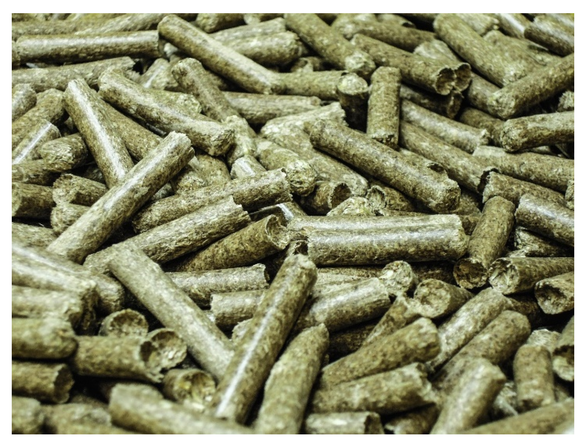
Cylindrical pellets made from energy grass black bent (Agrostis gigantea) were used in the experiments (Figure 1). Black bent is a medium-height (100 cm) winter perennial grass. It is used as a supplementary species in extensive permanent meadows and pasture grassland on heavier soils and wetlands. Black bent (Agrostis gigantea) was harvested in August 2017.

2.2. Methods

Dried grass was crushed in a pilot plant using a Green Energy 9FQ 50 hammer crusher and then pelleted on a Kahl 14-175 flat-die laboratory scale pellet press. The diameter of all cylindrical pellets was d = 6 mm. This sample was taken from a production cycle.

Pellet lengths were measured using a caliper gauge with an accuracy of 0.1 mm. A 1.5 kg batch consisting of 1600 pellets was manually measured.

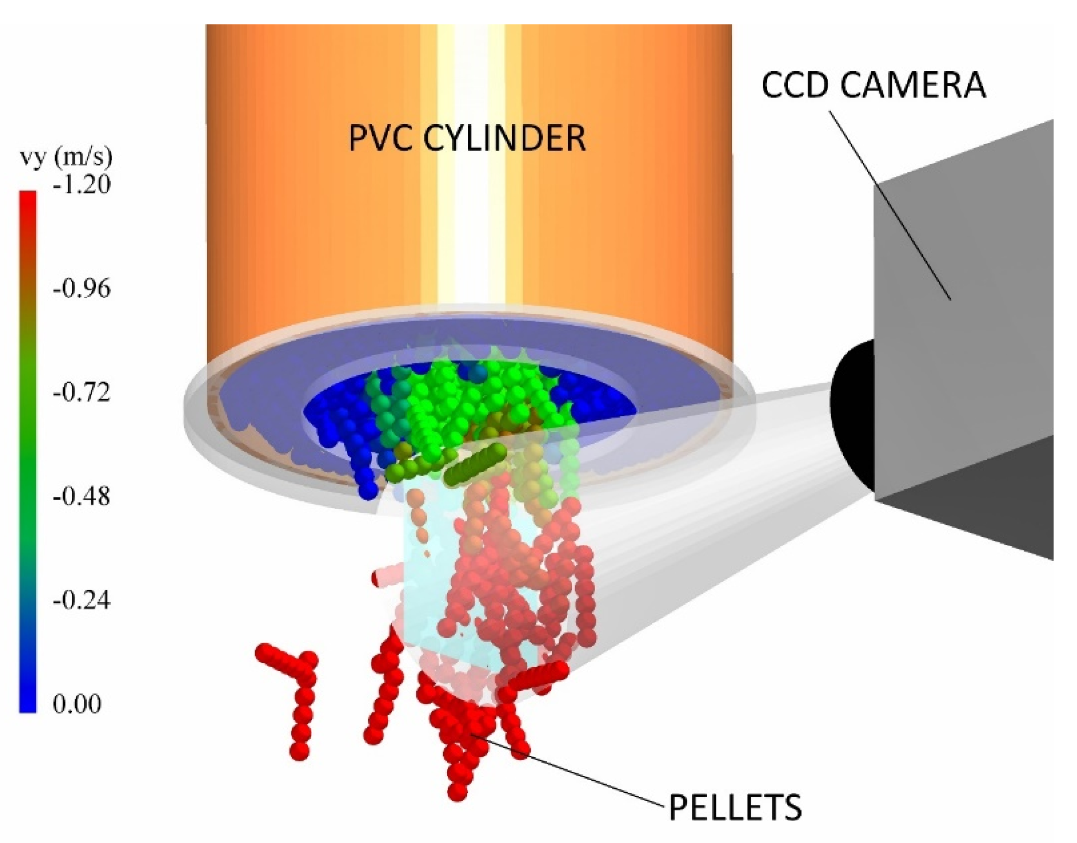
2.3. Experimental Procedure

A PVC cylinder with a flat plexiglass bottom was used in the experiments to ascertain the flow properties of the cylindrical pellets. The cylinder had an internal diameter of 152 mm and a height of 200 mm. The diameter of the outlet hole at the bottom was 100 mm.

All the measured cylindrical pellets were placed into the cylinder, which remained closed during filling. After the cylinder was filled, the outlet hole was opened, and the cylinder was allowed to discharge. The size of the outlet hole was selected so that the cylindrical pellets would not be obstructed from flowing throughout the entire cylinder discharge process. After the cylinder discharged, however, a small number of pellets remained in the cylinder, most likely because of the flat bottom. The flow of pellets from the cylinder was recorded with a high-speed camera. Filling, discharge and recording was repeated ten times. The experiment is illustrated in Figure 2.

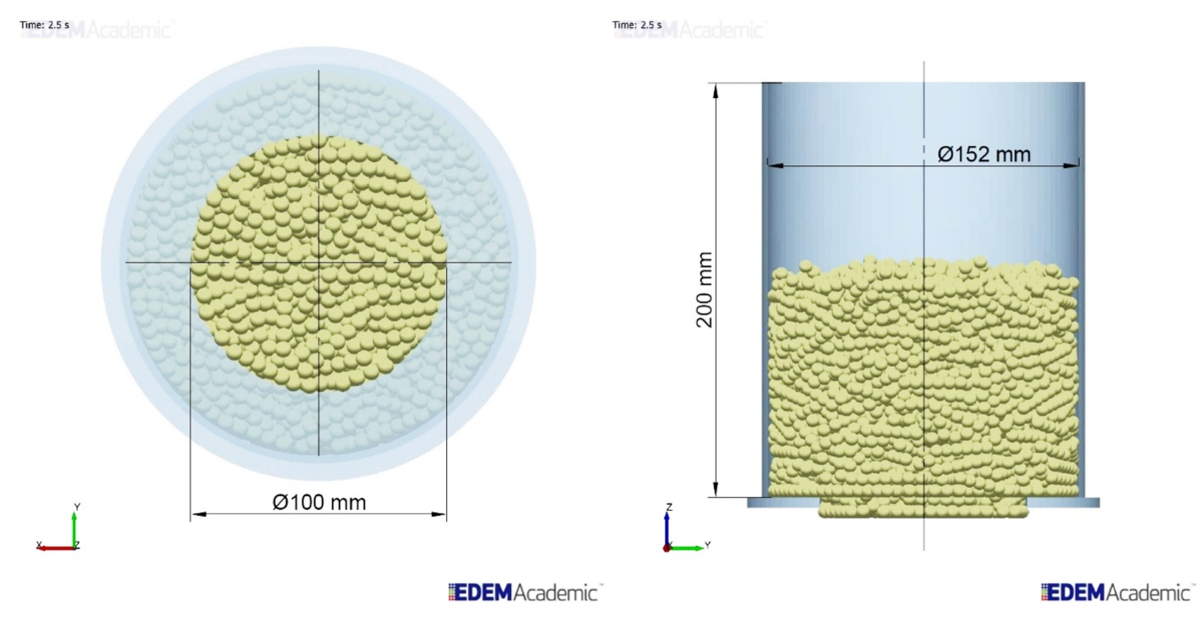
2.4. DEM Model

EDEM Academic software was used to simulate the experiments with the DEM. The basic geometric dimensions of the cylinder model are identical to the real model used for discharging the cylindrical pellets and PIV measurement. The DEM cylinder model is shown in Figure 3.

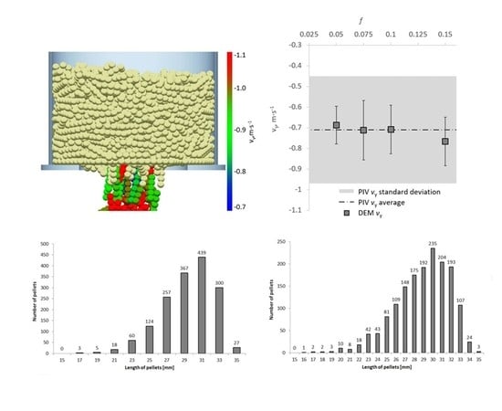
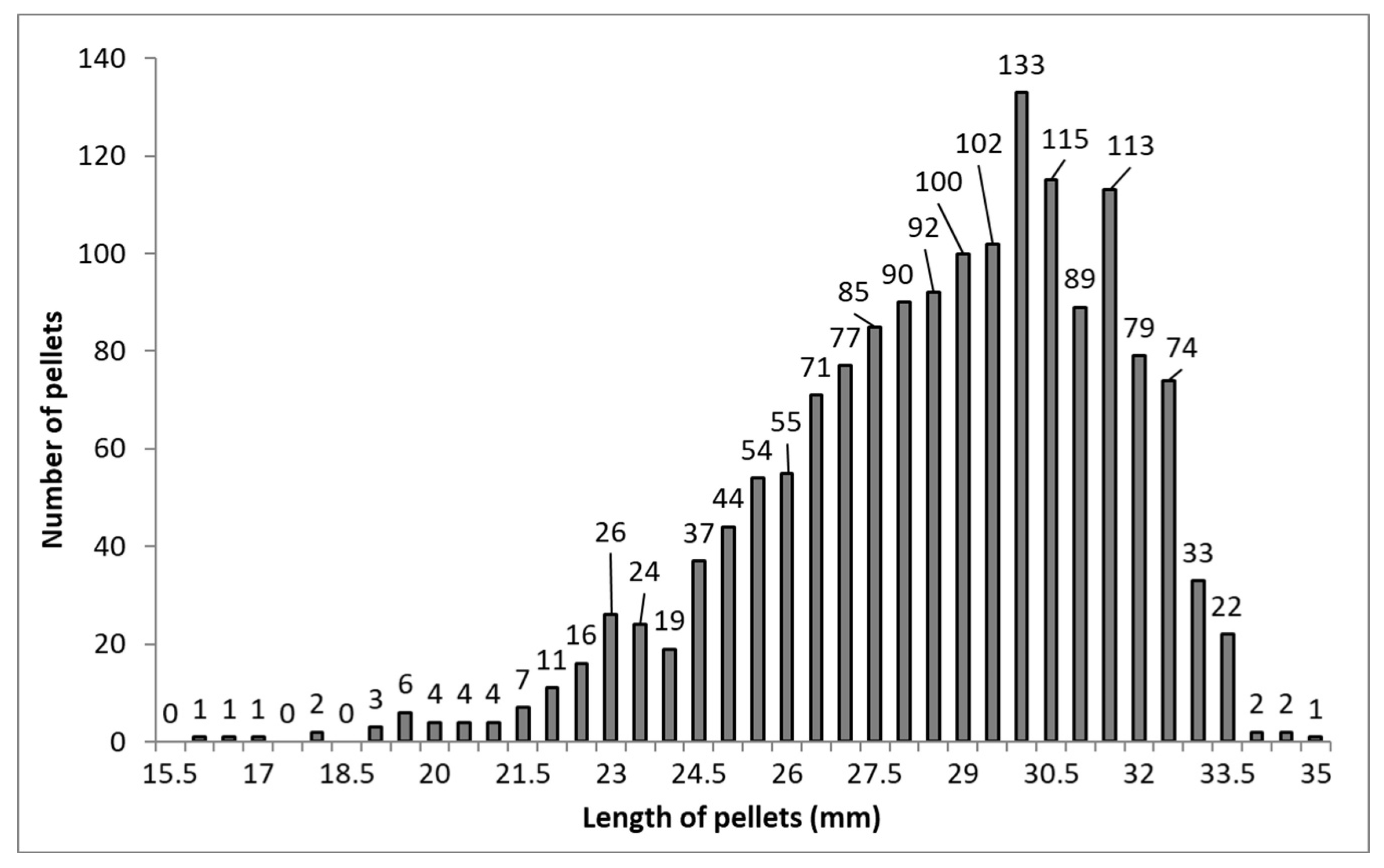
The primary pellet size distribution according to their actual measured lengths is shown in Figure 4, with a length accuracy grade of t₁ = 0.5 mm. The average length value of cylindrical pellets in the sample was L_p = 28.45 ± 2.93 mm. The standard deviation value of u = 2.93 mm according to normal Gaussian distribution is 10.3% of the average value of the measured length of cylindrical pellets L_p.

The most accurate grade of cylindrical pellet t₁ was derived from real measurements (as mentioned above).

The other two accuracy grades of cylindrical pellet, t₂ = 1 mm and t₃ = 2 mm, were derived from t₁, and a different step width was applied to them.

In this article, the length accuracy grade is the difference between the values of the two nearest size classes. The size class is a set of specific pellet lengths. If the degree of precision is 2 mm in length, the classes were graded in steps of 2 mm. For example, 21 mm, 23 mm and 25 mm. The length of the pellets ranges from 21.1 to 23 mm in the 23 mm class.

The input parameters for the DEM material properties are indicated in

Table 1. Material properties.

Input Parameter	Geometry	Pellet Material
Poisson’s Ratio (-)	0.25	0.33
Shear Modulus (Pa)	1.00 × 108	5.00 × 108
Density (kg·m−3)	2500	1564–1650

.

The high shear modulus values in Table 1 were used to achieve sufficient rigidity in individual particles [26]. Here, the values 1.00 × 10⁸–1.00 × 10⁹ did not affect the angle of repose or bulk density. For pellets, the shear modulus value was selected from approximately the centre of the 1.00 × 10⁸–1.00 × 10⁹ range. Poisson’s Ratio and the shear modulus was obtained from literature [27].

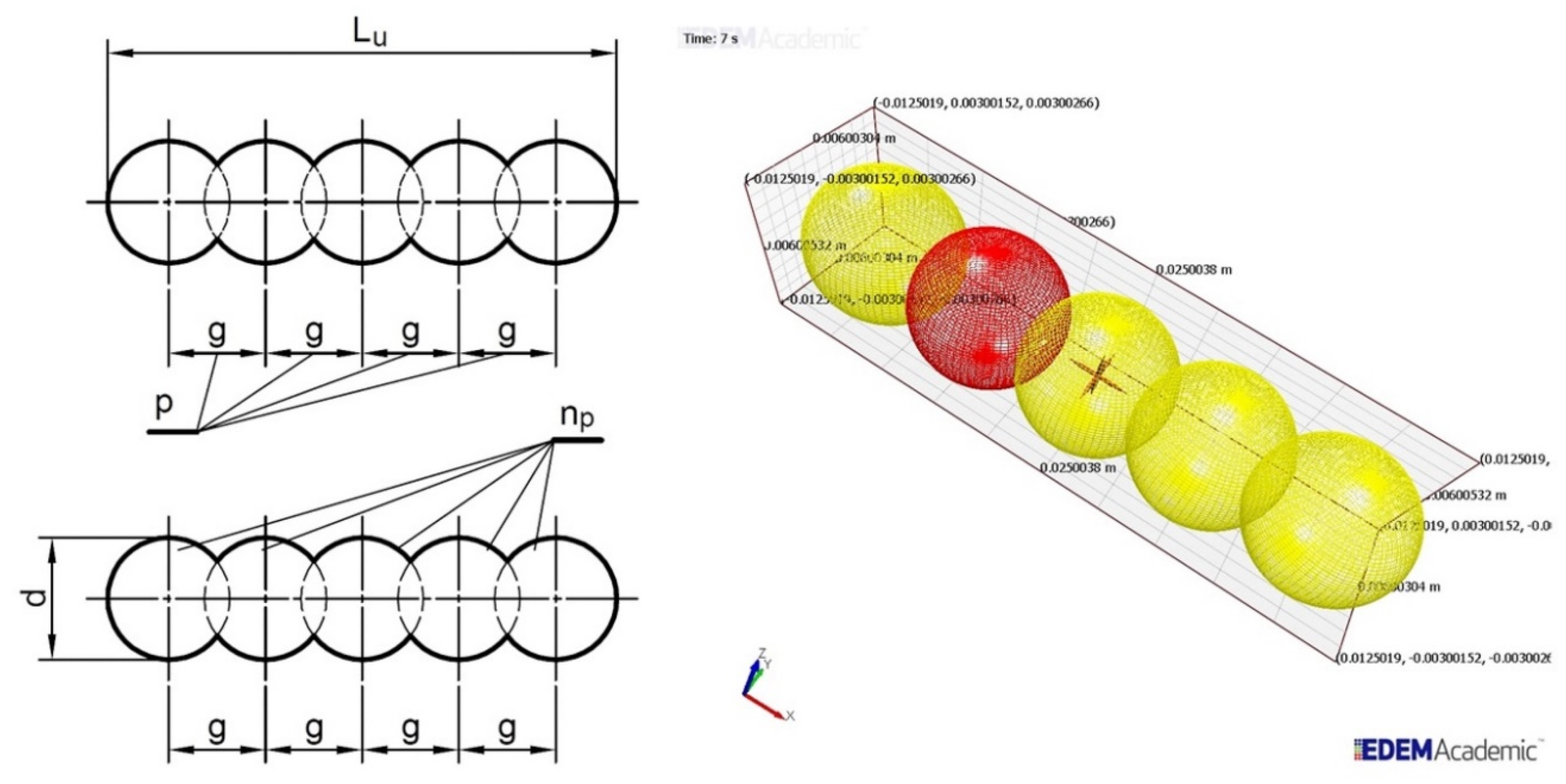
It was necessary to set the gap size between spherical particles in each cylindrical pellet, as well as the number of required spherical particles, as illustrated in Figure 5. This was based on the measured pellet length L_u. The number of spherical particles n_p making up the pellet was obtained by dividing the measured pellet length of L_u by the pellet diameter d, as given by Equation (1). This was rounded up to the nearest integer. The number of gaps between spherical particles p was calculated using Equation (2), and the gap size g was calculated using Equation (3).

$$n_p=\frac{L_u}{d}$$

(1)

$$p=n_p-1$$

(2)

$$g=\frac{L_u-d}{p}$$

(3)

The contact parameters for DEM simulations are given in

Table 2. Contact parameters.

Input Parameter	Pellet to Pellet	Pellet to Geometry
Coefficient of Restitution (-)	0.2	0.3
Coefficient of Static Friction (-)	0.005–0.15	0.15
Coefficient of Rolling Friction (-)	0	0

. Values for the pellets’ coefficient of restitution were selected. The character of the pellet flow in the container where the effect of the coefficient of restitution was not so dominant was also a prerequisite. Static friction coefficient values of f = 0.005, 0.0075, 0.1 and 0.15 were applied to pellet selection from t₁–t₃ marked as t₄–t₆ in the DEM, as shown below. These four friction values were used each time for each cylindrical pellet selection. For each friction coefficient in the DEM, ten simulations were performed. Forty simulations were performed for one length accuracy grade of the cylindrical pellets in the DEM. In all, a hundred and twenty simulations were performed. Physical interactions between the pellets and between the geometry and the pellets were according to Hertz-Mindlin (no slip) [12].

In general, the number of particles used in the simulation affected the simulation speed. A higher particle number increased the calculation time [18]. The specific lengths of these pellets were selected for DEM simulation of discharging the cylindrical pellets.

Three pellet selection (t₄–t₆) for the DEM were derived from the length accuracy grades of t₁, t₂ and t₃ (

Table 3. Pellet selection t₄, t₅ and t₆—lengths selected from t₁, t₂ and t₃ in the DEM model.

Lu (mm)	Pellet Selection	Number of Pellets (pcs)	g (mm)	np (pcs)
21	t6	18	5	4
22	t5	18	5.33	4
22.5	t4	16	5.5	4
23	t4, t5, t6	26, 42, 60	5.67	4
23.5	t4	24	5.83	4
24	t4, t5	19, 43	6	4
24.5	t4	37	4.63	5
25	t4, t5, t6	44, 81, 124	4.75	5
25.5	t4	54	4.88	5
26	t4, t5	55, 109	5	5
26.5	t4	71	5.13	5
27	t4, t5, t6	77, 148, 257	5.25	5
27.5	t4	85	5.38	5
28	t4, t5	90, 175	5.5	5
28.5	t4	92	5.63	5
29	t4, t5, t6	100, 192, 367	5.75	5
29.5	t4	102	5.88	5
30	t4, t5	133, 235	6	5
30.5	t4	115	4.9	6
31	t4, t5, t6	89, 204, 439	5	6
31.5	t4	113	5.1	6
32	t4, t5	79, 193	5.2	6
32.5	t4	74	5.3	6
33	t4, t5, t6	33, 107, 300	5.4	6
33.5	t4	22	5.5	6
34	t5	24	5.6	6
35	t6	27	5.8	6

). The derived t₄, t₅ and t₆ include simplification. Pellet sizes (lengths) with a value less than 1% of the total number of pellet samples were not included. The total number of pellets was 1600 (i.e., one percent being 16 pellets).

From the sample with a length accuracy grade of t₁, 23 sizes were taken. These pellets ranged from 22.5 mm to 33.5 mm in size (t₄, Table 3). From the sample with a length accuracy grade of t₂, 13 sizes were selected. These pellets ranged from 22 mm to 34 mm in size (t₅, Table 3). From the sample with a length accuracy grade of t₃, 8 sizes were selected. The pellets ranged from 21 mm to 35 mm in size (t₆, Table 3).

To obtain an assumed total weight of 1.5 kg in the DEM pellet sample, density values of 1650 kg·m⁻³ for t₄, 1628 kg·m⁻³ for t₅ and 1564 kg·m⁻³ for t₆ were used. These values were determined by direct correlation.

2.5. Particle Image Velocimetry

The camera frame rate was set to record at 500 frames per second. With a maximum resolution of 2016 × 2016 pixels and frequency of 500 fps, the CCD camera (LaVision Imager pro HS 4M) recorded 3600 pictures in a single shooting sequence, corresponding to a video length of 7.2 s. This interval was sufficient for all of the cylinder discharging process experiments. The recorded cylinder discharging process was evaluated using the PIV software DaVis 8.0.8 from the LaVision company. The aim was to determine the average components of vertical velocity v_y of the pellets in the area just outside the outlet hole. Particle Image Velocimetry (PIV) is an optical method used to visualize flow. The results of a PIV analysis are typically a two-dimensional vector field. The cross-correlation method (in Davis LaVision software) was used to evaluate the PIV data. The images were separated into regular windows of the same size. A velocity vector was determined in each of these windows. The software stacked the corresponding windows from the first and second time slots and then shifted the images toward each other. For each position, the software then counted the signal match rate in each individual pixel to form a correlation map. From the best matches, peaks were created, and the resulting vectors subsequently determined from their positions. In the final stage, the average velocity of pellet movement from a scanned area could be obtained using the Davis LaVision software.

The calibration was performed by linear scaling. In this way, the transfer of pixel to the length units (millimetres) and the coordinate system in the images were created directly in DaVis 8.0.8.

3. Results

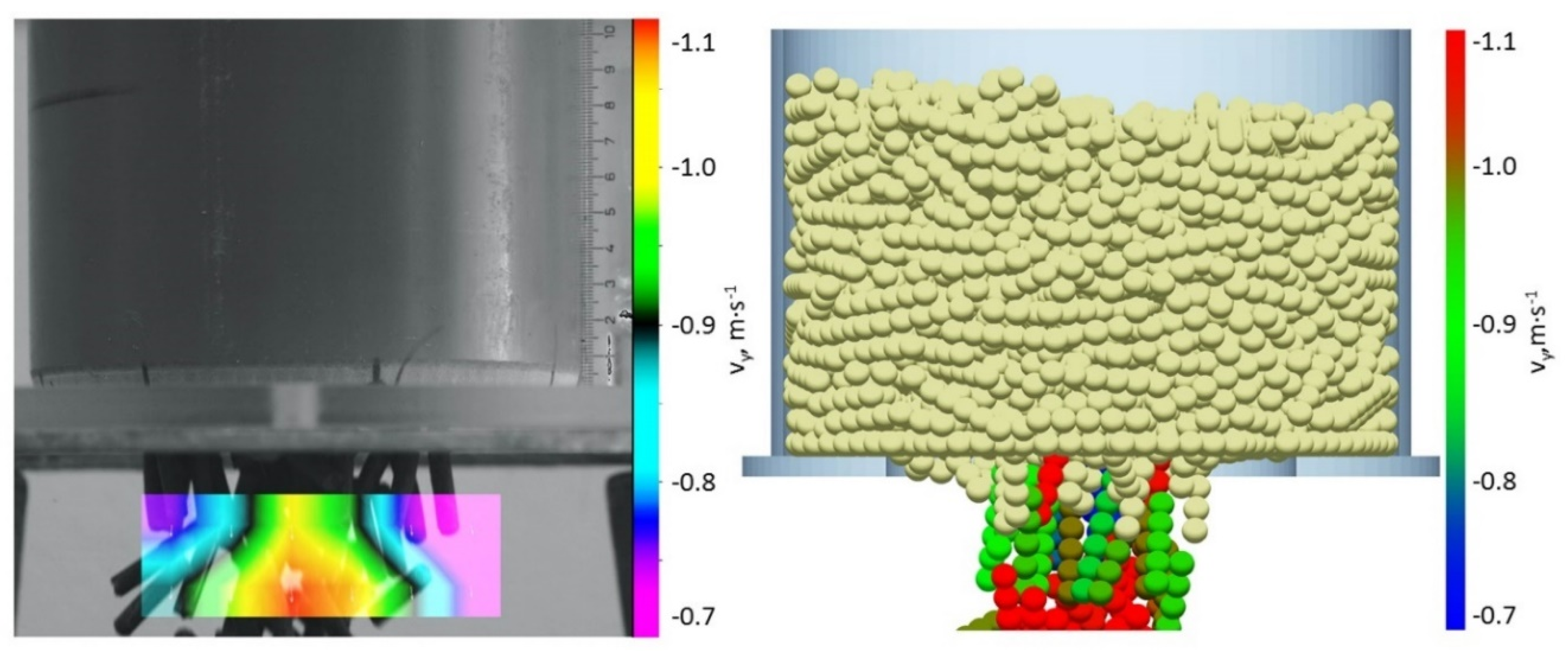
The objective of PIV and DEM measurement was to obtain average values of the vertical velocity component v_y and the discharge time t_e. Ten measurements with the same settings were repeated with PIV. The values v_y and t_e in both PIV and the DEM were evaluated at the moment 0.2 s after the outlet hole had opened. The reason for this was to exclude movement of the closure element at the cylinder’s opening from the video recording. This movement could have affected the PIV values of v_y near the vector field area. The vector field area just outside the outlet hole in the PIV and DEM is illustrated in Figure 6. The total average velocity of the ten repeated PIV measurements outside the outlet hole was −0.71 m·s⁻¹. The standard deviation was 0.26 m·s⁻¹. The average discharge process time observed from ten measurements was t_e = 3.05 s, and the standard time deviation was 0.65 s.

Comparison of the results of the DEM simulations and the PIV measurement for t₄–t₆ are given in Figure 7, Figure 8 and Figure 9. The individual figures show v_y just outside the outlet hole on the left, and the times t_e on the right. Four values of v_y and t_e are shown for frictions f = 0.05 to f = 0.15. Each v_y and t_e value in the DEM was created as an average of ten simulations. The standard deviation zones and average values of v_y and t_e in the PIV measurement are also indicated.

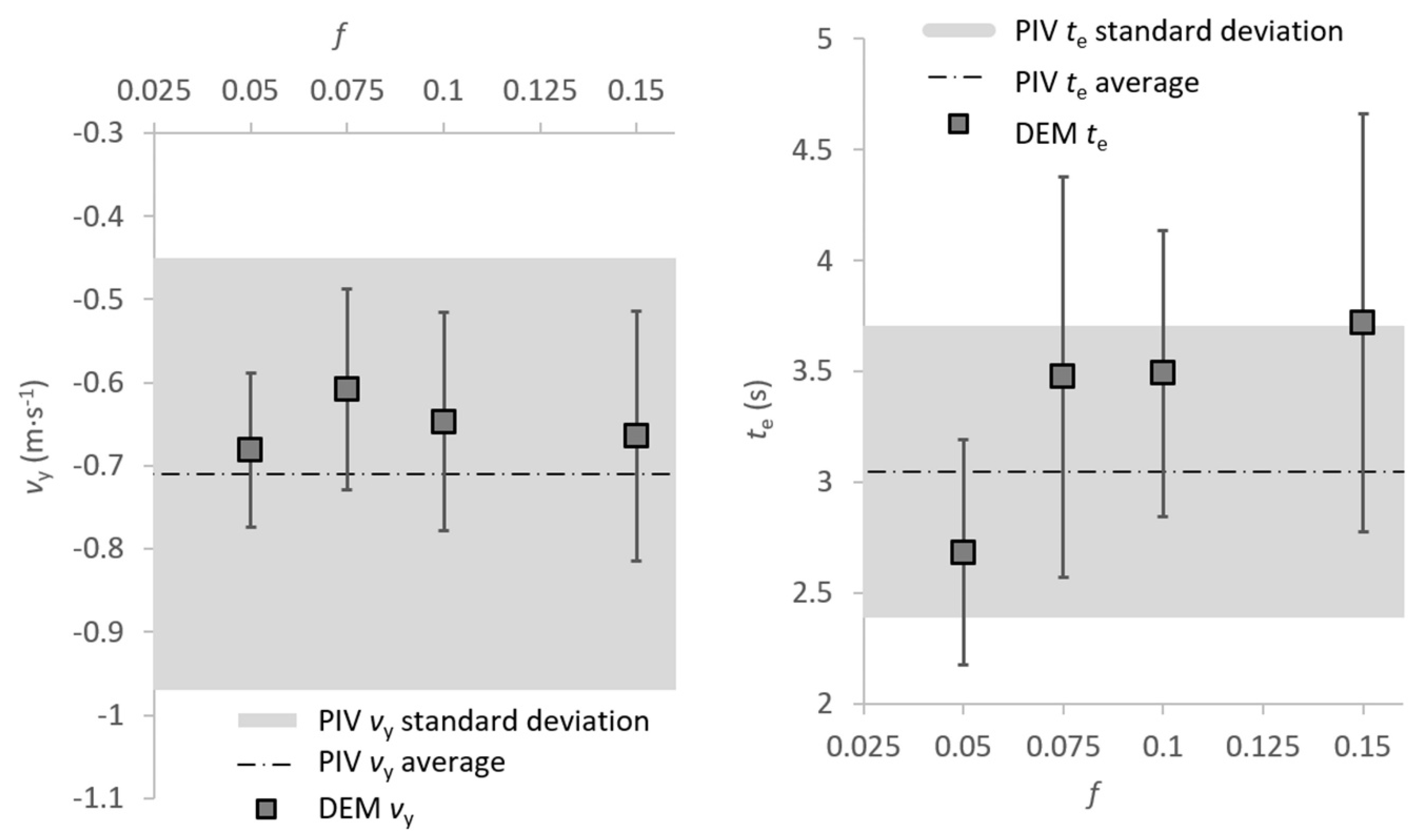
Figure 7 shows a graph of v_y just outside the outlet hole and time t_e for t₄ in the DEM from Table 3. The resultant DEM velocities v_y were near the average value from the PIV; the discharge times t_e; however, were different. The resultant combination of the pair of values v_y and t_e was best at a friction of f = 0.05. The highest deviation of the average value of t_e in the PIV simulations resulted in a friction of f = 0.15. The friction coefficient f between pellets shows a significant influence. As the friction coefficient f increased, the discharge time t_e increased. The difference between the highest and lowest average value of t_e was 1.04 s. The values of average velocities v_y in the DEM did not change distinctively as the friction f changed.

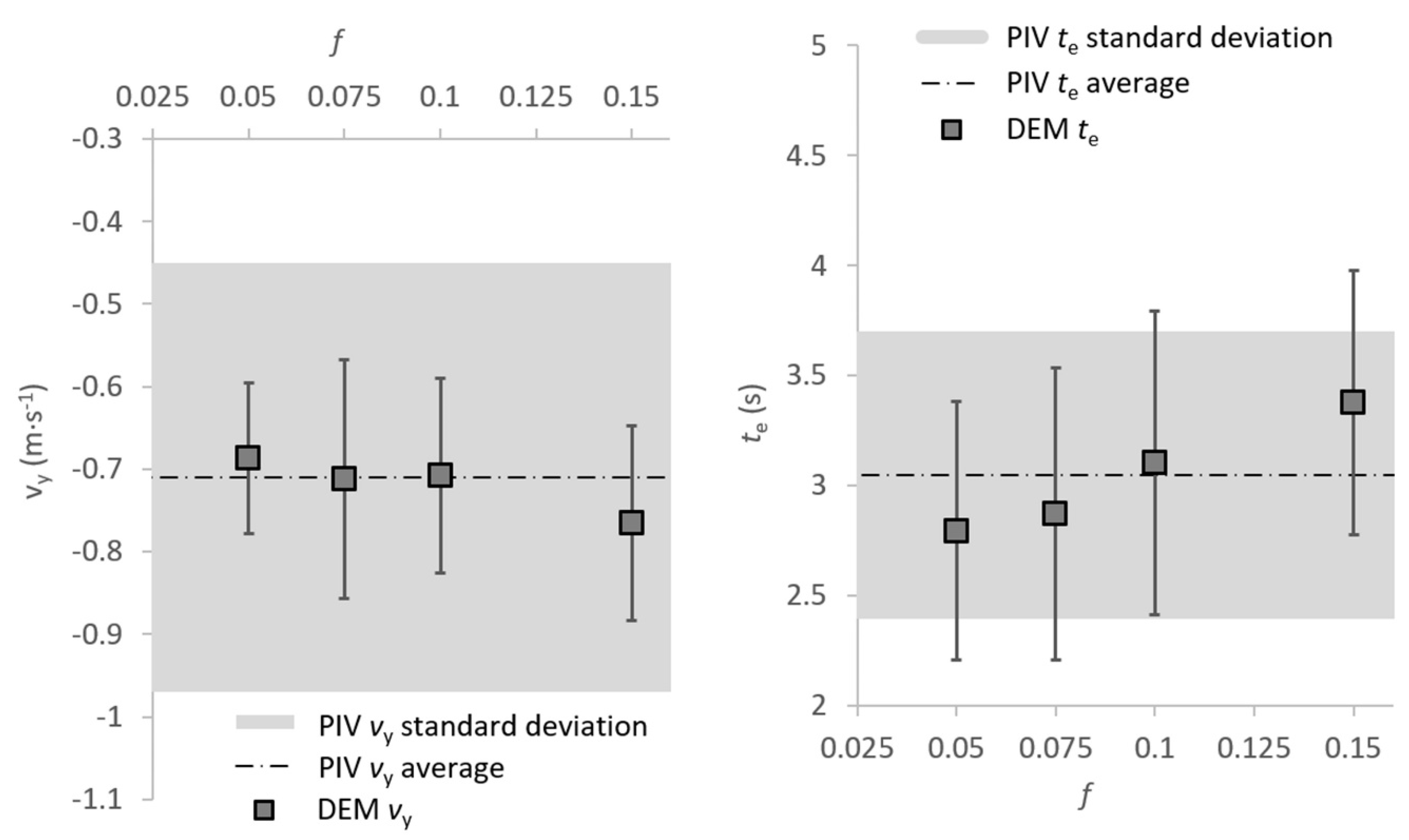
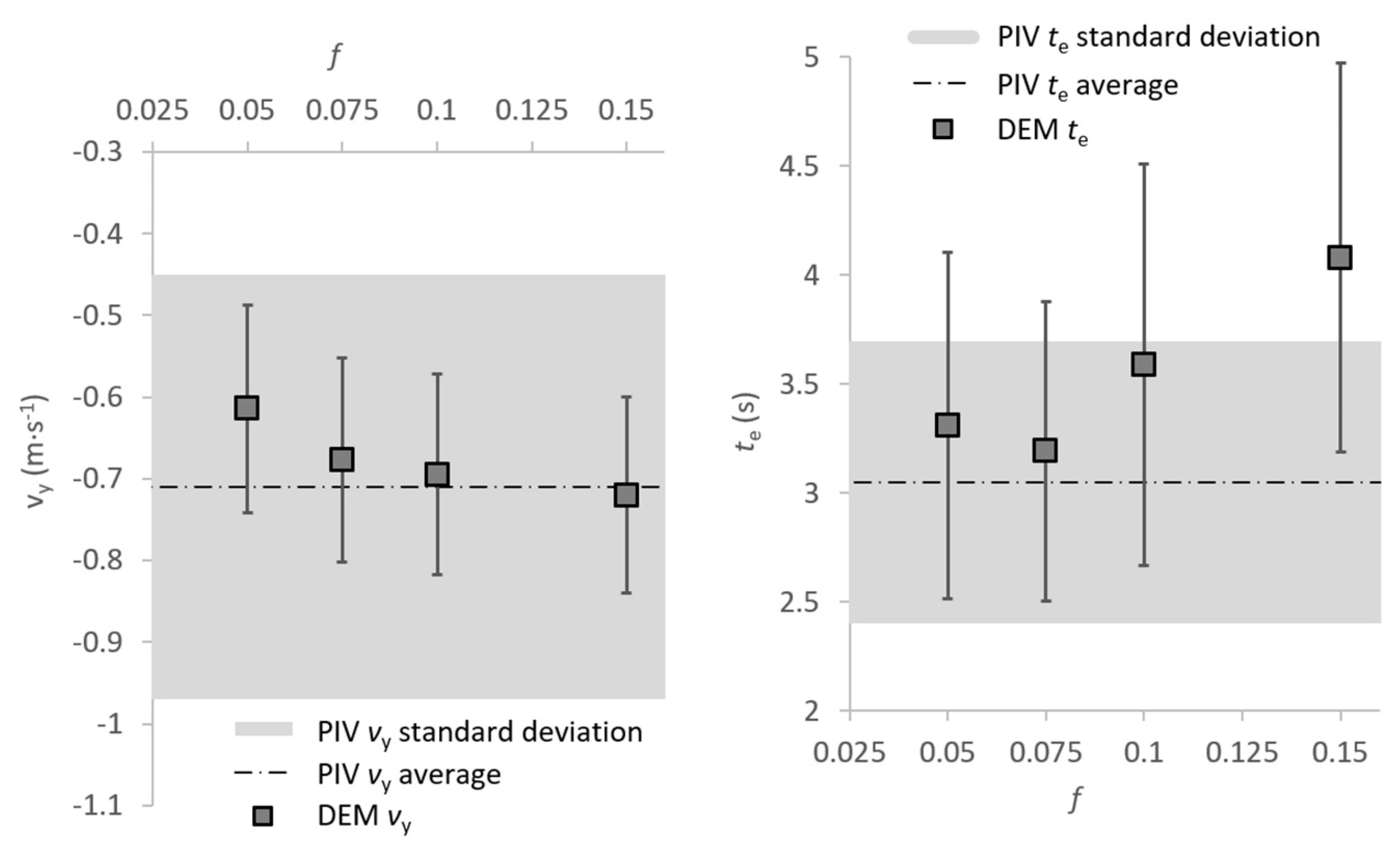
Figure 8 shows a graph of the vertical velocity component v_y just outside the outlet hole and time t_e for pellet selection t₅. The resultant DEM velocities v_y were near the average value from the PIV; the discharge times t_e, however, were different. The resultant combination of the pair of values v_y and t_e were optimal at friction f = 0.1.

The resulting average value of t_e from the simulations with a friction of f = 0.05 differed by 0.07 s from the result with f = 0.075. The obtained results reveal that t₅ was the most suitable of all the tested samples with a specific length accuracy grade. The resulting t_e for friction f of 0.05 to 0.1 had a similar character; the values did not differ from each other as much as in the case of samples t₄ and t₆. The difference between the average value of t_e from the PIV and the values in the DEM was a time of 0.25 s for friction f = 0.05, a time of 0.18 s for f = 0.075, a time of 0.05 s for f = 0.1, and a time of 0.33 s for f = 0.15. The difference between the average values between PIV and the DEM was highest at friction f = 0.15.

Figure 9 shows graphs of the vertical velocity component v_y just outside the outlet hole and time t_e for t₆. The resultant DEM velocities v_y were near the average value from the PIV; the discharge times t_e, however, were different. The highest average value of t_e was for friction f = 0.15.

The resulting average value of t_e in the DEM for f = 0.1 differed by 0.28 s from the result with f = 0.05. With regard to the average value v_y in the DEM, the result for f = 0.1 was better than that for f = 0.05; the average value of t_e in the DEM, however, was lower for f = 0.05 than for f = 0.1. The resulting average value t_e for friction f = 0.15, however, was higher for t₆ by 0.36 s than t₄. The difference between the average value of t_e in PIV and the values of t_e in the DEM was a time of 0.26 s for friction f = 0.05, a time of 0.14 s for f = 0.075, a time of 0.54 s for f = 0.1, and a time of 1.03 s for f = 0.15.

At first glance, from the values of pellet emptying times t_e and pellet velocity v_y, it follows that the optimal pellet model appears to be the case of t₅. This model showed the best range of velocities and times in the DEM across the whole range of friction coefficients. These values showed minimum dispersion (the least fluctuation) around the average values of the PIV measurements. The results of t_e for t₄ and t₆ differ most from the PIV with friction f = 0.15. Finding and examining the differences between the individual t₄–t₆ was necessary.

By comparing the values from Table 3, it was evident that t₅ was different to t₄ and t₆. All three pellet selections had pellets with 4, 5 and 6 particles, but t₅ had the largest proportion of four-particle pellets. t₅ had 1.21 times more than t₄ and 1.32 times more than t₆. The large impact these differences had and how it influenced the emptying time t_e for individual pellet selection with a friction setting of f = 0.15 was observed.

In the t_e comparison of t₄ with t₅ at a friction f = 0.15, a 20% difference can be seen in the proportion of the four-particle pellets already at the limit of the range of the average value in the PIV measurements. It could be said that a larger number of smaller particles had a positive effect on reducing friction (filling the space between larger pellets) and thus reduced time. All three created DEM pellet selections were suitable for validation. However, the usable limit was at f = 0.15. This limit is especially significant in pellet selection t₆. If the applied DEM pellet model had been calibrated to friction values even higher than f = 0.15, granulometry t₆ would probably not have been suitable.

4. Conclusions

This article compared the DEM simulations with the PIV results and determined the influence of the length accuracy grade of the pellets on the velocity and time during discharge of the hopper.

The DEM measurements revealed that verification of the hopper discharge process using PIV cannot be evaluated by knowing the velocity parameter v_y only. An important role is played by the discharge time t_e and the friction coefficient f that affects this time in determining the accuracy of the results.

The necessary friction coefficient f was set so that the resultant average values of v_y in the DEM were very close to the average values of v_y in PIV. The criterion to determine the accuracy of the results was the value of the discharge time t_e.

Three DEM pellet samples were created with different length accuracy grades and numbers of individual pellet sizes.

The sample with t₄ had the highest number of pellet length sizes, from which 23 sizes were selected. From the sample with t₅, 13 length sizes were selected. From the sample with t₆, 8 pellet length sizes were selected. The pellet selections contained a different number of the smallest particles.

Pellet selection t₅ contained the largest proportion of four-particle pellets. Compared to granulometry, t₅ had 1.21 times more than t₄ and 1.32 times more than t₆. The impact these differences had and how it influenced the emptying time t_e for individual granulometries with a friction setting of f = 0.15 was determined.

In the DEM simulations, the friction between pellets was set from f = 0.05 to f = 0.15. In all cases, time t_e increased as f increased. For correct calibration of t₄, the most optimal friction coefficient was f = 0.05. For sample t₅, the optimum friction coefficient was f = 0.1. For t₆, it was f = 0.075.

The most accurate average value of t_e in the DEM simulation compared to t_e from the PIV was observed in t₅ at friction coefficient f = 0.1. This setting can be regarded as the best in terms of DEM calibration in the given case.

It was discovered that a larger number of smaller particles had a positive effect on reducing friction and thus reduced the time t_e. All three DEM pellet selections were suitable for validation. However, the usable limit was at friction coefficient f = 0.15, especially for t₆. If the applied DEM pellet model had been calibrated to friction values even higher than f = 0.15, t₆ would probably not have been suitable.