Evolutionary Observer Ensemble for Leak Diagnosis in Water Pipelines

Abstract

This work deals with the Leak Detection and Isolation (LDI) problem in water pipelines based on some heuristic method and assuming only flow rate and pressure head measurements at both ends of the duct. By considering the single leak case at an interior node of the pipeline, it has been shown that observability is indeed satisfied in this case, which allows designing an observer for the unmeasurable state variables, i.e., the pressure head at leak position. Relying on the fact that the origin of the observation error is exponentially stable if all parameters (including the leak coefficients) are known and uniformly ultimately bounded otherwise, the authors propose a bank of observers as follows: taking into account that the physical pipeline parameters are well-known, and there is only uncertainty about leak coefficients (position and magnitude), a pair of such coefficients is taken from a search space and is assigned to an observer. Then, a Genetic Algorithm (GA) is exploited to minimize the integration of the square observation error. The minimum integral observation error will be reached in the observer where the estimated leak parameters match the real ones. Finally, some results are presented by using real-noisy databases coming from a test bed plant built at Cinvestav-Guadalajara, aiming to show the potentiality of this method.

1. Introduction

Fluid transport is a significant issue in the world today. Currently, cities are continually demanding utilities, including drinking water, the distribution of oil products, the treatment of wastewater, etc., and pipelines are predominantly used to do this. The pipeline networks have increased the growth and comfort of society. Nevertheless, there is also a constant risk (in particular, for fuel pipelines) that accidents, environmental pollution or economic losses may occur if the fluid spreads through leaks. In this context, several critical incidents have recently occurred within Mexico, such as San Martín Texmelucan, Puebla in 2010, and more recently in the Tuxpan-Tula poly-duct in the municipality of Tlahuelilpan, Hidalgo in 2019, where many people died as a result of an explosion caused by illegal fuel extraction. On the other hand, according to the National Water Committee (CONAGUA) [1], about 40% of drinking water is lost due to leakage. Although there are entirely different explanations for each problem, both can be solved by using similar techniques.

The scientific community has paid attention to that problem and has proposed several methodologies for monitoring and supervision purposes in order to avoid losses and accidents (see, e.g., [2,3,4,5,6,7,8,9,10,11]). In particular, in Begovich et al. [2], a LDI algorithm based on Billman and Isermann [3] has been implemented and tested with accurate results and based on steady-state conditions, which increase the convergence time in the leak parameter estimation process. The proposal in Verde et al. [5] deals with the location of multiple leaks in a pipeline. The key to the leak detector, which should operate in quasi-real-time, is a family of parameterized transient models for all scenarios in the pipeline. In this case, the equivalence in the steady-state of a leak at a position with two leaks allows obtaining the family of dynamic models. Then, to estimate the specific parameter of the leak, an off-line identification process is performed.

Likewise, a multi-leak diagnostic scheme has been suggested in Delgado-Aguiñaga et al. [4] based on Kalman observers. In general, it considers a model-based approach for detecting and isolating several non-concurrent leaks. The method modifies the nonlinear model for each new leakage event. Thus, it is an extension of the single-leak isolation problem. Although this scheme shows acceptable results, the complexity of computation increases as an additional leak occurs. In Rubio Scola et al. [12], the authors presented the development of a nonlinear state observer to locate a blockage in a pipeline. The technique uses a mathematical model derived from the equations of the water hammer together with the method of finite differences for its solution, providing a suitable location for the blockage. Besides, concerning the implementation problem, a recent algorithm based on the extended Kalman filter Delgado-Aguiñaga and Begovich [10] has successfully identified a leak in an aqueduct in Guadalajara, Mexico. A posterior study estimated that approximately 130 million liters of drinking water had been lost in this incident.

There are also other methods with successful application. For example, the approach presented in Ostapkowicz [6] uses a pressure wave method, and Liu et al. [11] presented a system based on acoustic waves. A hybrid approach based on a real-time transient simulation system, and a negative pressure wave method is proposed in Zhang et al. [7]. In the last reference, the authors argued that the most likely future development in pipeline leak detection and location tends to be the use of two or more different methods. Finally, Tian et al. [8] proposed an algorithm to locate leaks based on the pressure difference profile along the pipeline. It considers the effect of the static pressure increases at the leakage point.

On the other hand, analytical redundancy methods (the technique of several model-based methods) have demonstrated to be useful to improve the precision, reliability, and performance of a system. Notably, in the field of fault detection and isolation, the attention on this class of methods has increased lately in several topics, such as robotics Lyu et al. [13], control theory Chouchane et al. [14], diagnosis system Lunze [15], and the application of evolutionary algorithms and neural networks to fault diagnosis Witczak [16]. In particular, several works dealing the leak diagnosis problem in Water Distribution Networks (WDN) have also been proposed on the basis of genetic algorithms. In Vitkovsky et al. [17], a technique in conjunction with the inverse transient method is used to detect leaks and friction factors. Additionally, in [18], a model calibration process is formulated as an nonlinear optimization problem that is solved by using a genetic algorithm. Case studies are presented to demonstrate how the integrated approach is applied to water leak detection.

The framework previously stated encourages researchers to propose new model-based approaches that can be used in combination with other methods and thus contribute to the development of a robust leak diagnostic tool for single pipelines on the basis of analytical redundancy model.

By relying on an observability property, fulfilled for the single leak case, our approach considers building an observer ensemble together with a genetic algorithm to minimize the observation error and, in this way, estimate the leak parameters, i.e., position and magnitude. The extended Luenberger observer has been chosen to estimate the internal state variable (the pressure at the leak point). Such an observer is exponentially stable only if the parameters of the model are known. Otherwise, the observation error is, at last, uniformly ultimately bounded. Then, if only leak position and magnitude are the unknown parameters (the rest of the pipeline mathematical model parameters are well-known), it is possible to design a bunch of observers, each with different values of leak position and magnitude (the search space). Thus, the best estimation of the leak parameters provided by the observer ensemble is the one that gives the minimum residual. Now, the potential of the genetic algorithm could be exploited to find the best estimation of such parameters.

The paper is organized as follows. Section 2 provides the mathematical model. Section 3 describes the Leak Detection and Isolation scheme. Section 4 presents some successful experimental results. Finally, in Section 5, some conclusions and future work are discussed.

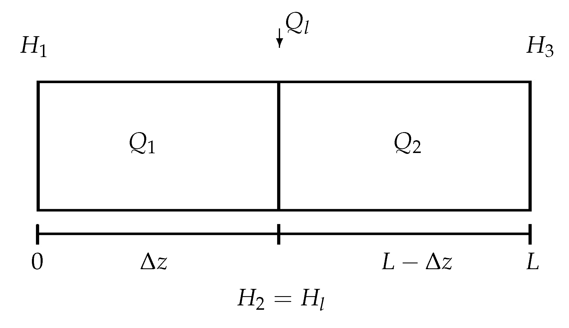
2. Pipeline Mathematical Model

The pipeline model is classically derived under the following assumptions: the pipeline is considered to be straight without any fitting and without slope; the fluid is slightly compressible; the duct wall is slightly deformable; and the convective velocity changes are negligible. Likewise, the pipeline cross-section area and fluid density are constant. Then, the Partial Differential Equations (PDE) governing the fluid transient response, can be written as Roberson et al. [19]:

Momentum Equation

$$\frac{\partial Q(z,t)}{\partial t}+g{A}_r\frac{\partial H(z,t)}{\partial z}+\mu Q(z,t)\left|Q(z,t)\right|=0$$

(1)

Continuity Equation

$$\frac{\partial H(z,t)}{\partial t}+\frac{b^2}{g{A}_r}\frac{\partial Q(z,t)}{\partial z}=0$$

(2)

where Q is the flow rate $[m^3/s]$; H is the pressure head $\left[m\right]$; z is the length coordinate $\left[m\right]$; t is the time coordinate $\left[s\right]$; g is the gravity acceleration $[m/s^2]$; $A_r$ is the cross-section area $\left[m^2\right]$; b is the pressure wave speed in the fluid $[m/s]$; $\mu =f\left(Q\right)/2\varphi A_r$, where $\varphi$ is the inner diameter $\left[m\right]$ and f is the friction factor; and the rest of physical parameters are computed as in Delgado-Aguiñaga et al. [20] considering a constant water temperature of 20 ${}^{\circ }\mathrm{C}$. The dynamics in Equations (1) and (2) is fully defined by related pairs of initial and boundary conditions.

Leak model: Furthermore, one leak arbitrarily located at point $z\in (0,L)$ (where L is the total length of the pipeline), can be modeled as follows Roberson et al. [19] (see Figure 1):

$$Q_l=\lambda \sqrt{H_l}$$

(3)

where the constant $\lambda$ is function of the orifice area and the discharge coefficient (for simplicity, the $\lambda$ coefficient is referred as “leak magnitude” from now on); $Q_l$ is the flow through the leak; and $H_l$ is the head pressure at the leak point Navarro et al. [21].

This leak produces a discontinuity in the system. Furthermore, due to the law of mass conservation, $Q_l$ must satisfy the next relation:

$$Q_2=Q_1+Q_l$$

(4)

where $Q_1$ and $Q_2$ are the flows before and after of the leak point, respectively.

Friction model: In modern pipes (pipes with a relative roughness usually less than $1\times {10}^{-3}$), it is difficult to reach a complete turbulence zone (i.e., the zone where friction factor is almost constant, see Figure 2).

Therefore, a friction factor deemed as a constant value could yield a poor mathematical model. For this reason, in the present work, the friction factor is calculated by using the well-known Swamee–Jain equation Brkić [22], Swamee and Jain [23]:

$$f\left(Q\right)=\frac{0.25}{{\left[{\mathit{log}}_{10}\left(\frac{ϵ}{3.7D}+\frac{5.4}{R{e}^{0.9}}\right)\right]}^2}$$

(5)

which is suitable for flow regime in the transition zone (as occurs in plastic pipelines) and where $ϵ\in \left[0.000001,0.05\right]$ [m] is the roughness height, $Re\in \left[5000,{10}^8\right]$ is the Reynolds number given by

$$Re=\frac{QD}{vA}$$

and v is the kinematic viscosity [m${}^2$/s].

Spatial Discretization of the Modeling Equations

In order to obtain a finite dimensional model from (1) and (2), such PDE’s are discretized with respect to the spatial variable z, as in Verde [24], Besançon et al. [25], by using the following relationships:

$$\frac{\partial H(z_i,t)}{\partial z}\backsimeq \frac{H_{i+1}-H_i}{z_i}\forall i=1,\cdots ,n$$

(6)

$$\frac{\partial Q(z_{i-1},t)}{\partial z}\backsimeq \frac{Q_i-Q_{i-1}}{z_{i-1}}\forall i=2,\cdots ,n$$

(7)

where $H_i$, $Q_i$ stand for $H(z_i,t)$, $Q(z_i,t)$, and n the number of pipeline sections. Assuming only one partition in the pipeline, as shown in Figure 1, $z_i$ ($i=1,2$) becomes the distance from upstream to the point of the leak and from the point of the leak to downstream, respectively. Notice that $\Delta z=z_1$ and $z_2=L-\Delta z$. The leak position is assumed to be $\Delta z\in (0,L)$ in this description. Applying the approximations in (6) and (7) to equations (1) and (2) together with (3), we get:

$$\left[\begin{array}{c}{\dot{x}}_1\\ {\dot{x}}_2\\ {\dot{x}}_3\end{array}\right]=\left[\begin{array}{c}-\frac{A_{r}g}{\Delta z}(x_2-u_1)-{\mu }_1{x}_1\left|x_1\right|\\ -\frac{b^2}{A_{r}g\Delta z}(x_3-x_1+\lambda \sqrt{x_2})\\ -\frac{A_{r}g}{L-\Delta z}(u_2-x_2)-{\mu }_2{x}_3\left|x_3\right|\end{array}\right]$$

(8)

Here, the state vector is defined as $x={\left[x_1{x}_2{x}_3\right]}^T={\left[Q_1{H}_2{Q}_2\right]}^T$, the input vector is $u={\left[u_1{u}_2\right]}^T={\left[H_1{H}_3\right]}^T$, and the pressure output vector is $y={\left[x_1{x}_3\right]}^T={\left[Q_1{Q}_2\right]}^T$, ${\mu }_i=f\left(Q_i\right)/2\varphi A_r$ with $i=1,2$. It is worth noting that $H_2$ represents the pressure head at the leak point. This value is impossible to measure since the leak position is not known “a priori”, but this value could be observed because, for the system (8), the observability property is fulfilled, as seen in the next section.

Notice that the mathematical model in (8) assumes a straight pipe without loss of generality, as, even if the pipe is not straight, it is possible to obtain an Equivalent Straight Length (ESL) of the pipe. This is done by considering losses due to each “non-straight element” (i.e., fitting). The equivalent straight pipe $L_e$ can be calculated as Mott [26]:

$$L_e=L_r+\frac{D{\sum }_{j=i}^n{K}_j}{f}$$

(9)

where $L_r$ stands for the pipeline physical length [m] measured between the sensors placed at the ends of the pipeline, $K_j$ is the fitting loss coefficient for the jth fitting, and n the total number of the pipeline fittings.

3. LDI Scheme Approach

The leak diagnosis process (the task of determining the magnitude $\lambda$ and location $\Delta z$ of the leak) proposed in this work is carried out by the design of a bank of observers together with a genetic algorithm method whose selection rule is to minimize the integration error of each observer.

Since the observability property of the system (8) is fulfilled, it is possible to design an extended Luenberger observer to estimate $H_2$. Such an observer is exponentially stable only if the parameters of the model ($A_r$, g, b, L, ${\mu }_1$, ${\mu }_2$, $\lambda$, and $\Delta z$, in (8)) are known; otherwise, the observation error will be uniformly ultimately bounded. Then, if only leak position ($\Delta z$) and magnitude ($\lambda$) are the unknown parameters (the rest of the pipeline mathematical model parameters are known), it is possible to design a bunch of observer, s each with different values of $\lambda$ and $\Delta z$, i.e., search space. Thus, the best leak position and leak magnitude estimation of the ensemble is the one that gives the minimum residual. Now, the potential of the genetic algorithm could be exploited to find the best estimation of such parameters.

The minimum integral observation error will be reached when the leak position and magnitude match the real ones.

3.1. Extended Luenberger Observer for MIMO Systems

First, let us consider that the space-state representation given by (8) can be rewritten in compact form:

$$\begin{array}{c}\hfill \dot{x}=f(x,u)\hfill \\ \hfill y=h\left(x\right)\hfill \end{array}$$

(10)

with the state $x\in {\mathbb{R}}^3$, the input $u\left(t\right)\in {\mathbb{R}}^2$, and the output $h\left(x\right)\in {\mathbb{R}}^2$ (with two components, $h_1$ and $h_2$). Then, the observability is guaranteed by invertibility of the following map (where $L_f$ denotes the Lie derivative):

$$Y=\left[\begin{array}{c}{y}_1\\ {\dot{y}}_1\\ y_2\end{array}\right]=\left[\begin{array}{c}{h}_1\\ L_f{h}_1\\ h_2\end{array}\right]=\left[\begin{array}{c}{x}_1\\ -\frac{A_{r}g}{\Delta z}(x_2-u_1)-{\mu }_1{x}_1\left|x_1\right|\\ x_3\end{array}\right]$$

(11)

which is in fact uniform in u. If one considers $x_1\left|x_1\right|=x_1^2$ (for unidirectional flow), such a map induces the following rank observability condition:

$$rank\left(\frac{\partial Y\left(x\right)}{\partial x}\right)=\left[\begin{array}{ccc}1& 0& 0\\ -2{\mu }_1{x}_1& -\frac{A_{r}g}{\Delta z}& 0\\ 0& 0& 1\end{array}\right]=3$$

(12)

such that the system in (10) is locally observable and satisfies the condition for the extended Luenberger observer design for MIMO systems Birk and Zeitz [27]. Then, the system (10) can be rewritten to obtain its additive output nonlinearity form:

$$\begin{array}{c}\hfill \dot{x}=Ax+\phi \left(x\right)+\varphi \left(u\right)+\xi \left(y\right)\hfill \\ \hfill y=Cx\hfill \end{array}$$

(13)

where matrices A, $\phi \left(x\right)$, $\varphi \left(u\right)$, $\xi \left(y\right)$, and C are given by:

$$A=\left[\begin{array}{ccc}0& -\frac{a_1}{\Delta z}& 0\\ \frac{a_2}{\Delta z}& 0& -\frac{a_2}{\Delta z}\\ 0& \frac{a_1}{L-\Delta z}& 0\end{array}\right]\phi \left(x\right)=\left[\begin{array}{c}0\\ -a_2\frac{\lambda }{\Delta z}\sqrt{x_2}\\ 0\end{array}\right]$$

$$\varphi \left(u\right)=\left[\begin{array}{c}\frac{a_1}{\Delta z}{u}_1\\ 0\\ -\frac{a_1}{L-\Delta z}{u}_2\end{array}\right]\xi \left(y\right)=\left[\begin{array}{c}-\mu y_1\left|y_1\right|\\ 0\\ -\mu y_2\left|y_2\right|\end{array}\right]$$

$$C=\left[\begin{array}{ccc}1& 0& 0\\ 0& 0& 1\end{array}\right]$$

where $a_1\dot{=}{A}_{r}g$ and $a_2\dot{=}\frac{b^2}{A_{r}g}$. Here, the additive output nonlinearity can be built from direct measurements and thus compensated in the observer design (as it was originally proposed by the authors in Krener and Isidori [28], J. Krener and Respondek [29], for instance). The representation (13) admits an observer of the form:

$$\begin{array}{c}\hfill \dot{\widehat{x}}=A\widehat{x}+\phi \left(\widehat{x}\right)+\varphi \left(u\right)+\xi \left(y\right)+K(y-C\widehat{x})\hfill \\ \hfill \widehat{y}=C\widehat{x}\hfill \end{array}$$

(14)

By defining the estimation error as $e=x-\widehat{x}$, the dynamic error model is:

$$\dot{e}=(A-KC)e+{\phi }^{\prime }(x,\widehat{x})$$

(15)

where ${\phi }^{\prime }(x,\widehat{x})={\left[\begin{array}{ccc}\hfill 0& -a_2\frac{\lambda }{\Delta z}(\sqrt{x_2}-\sqrt{\widehat{x_2}})& 0\hfill \end{array}\right]}^T$.

In this equation, $e=0$ is clearly an equilibrium. In addition, K can be chosen so that $(A-KC)$ is Hurwitz (since $(A,C)$ is observable), that is for any $Q=Q^T>0$, there exists $P=P^T$ satisfying the Lyapunov equation $P(A-KC)+{(A-KC)}^{T}P=-Q$.

Notice then that $\phi (x,\widehat{x})$ satisfies a linear growth bound $\parallel \phi (x,\widehat{x})\parallel \le \gamma \parallel e\parallel$ on the region of operation, and thus if $\gamma <{\zeta }_{min}\left(Q\right)/2{\zeta }_{max}\left(P\right)$, where ${\zeta }_{min}(·)$ and ${\zeta }_{max}(·)$ denote the minimum and maximum eigenvalue of a matrix, one can conclude that the origin of the error system in (13) is exponentially stable (see Khalil [30] for more details).

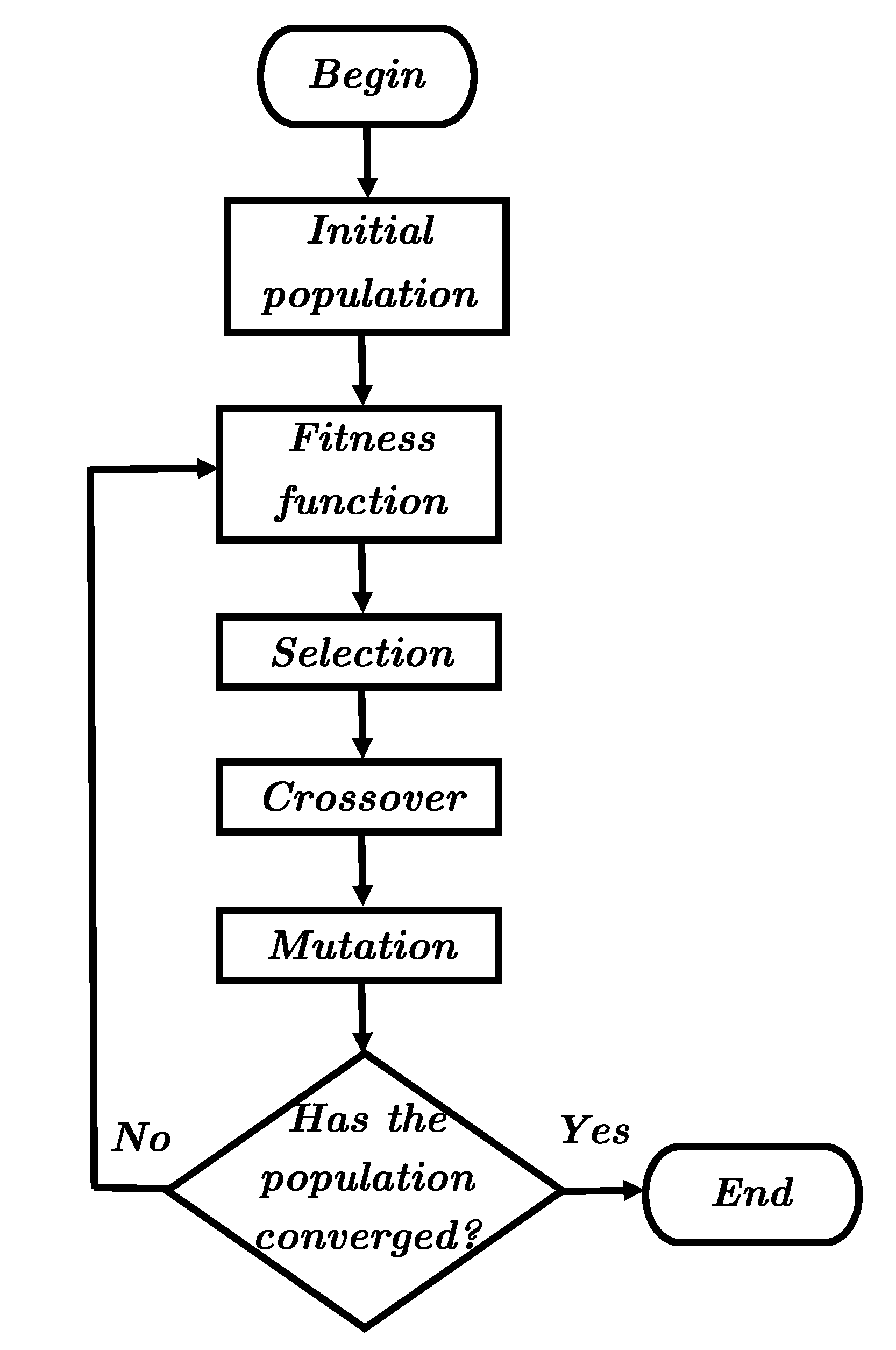
3.2. Genetic Algorithm

In computer science, the genetic algorithm is an algorithm inspired in the biological evolution that offers a suitable solution to optimization and search problems. The GA is a recursive algorithm where the aptest individuals of a population are discovered, emphasized, and recombined (reproduction) in order to produce descendants of the next generation. Six phases are considered in a genetic algorithm:

• Initial population. The first step of the process is to obtain a set of individuals randomly generated (initial population) in which each such individual is a candidate solution to a problem.
  As in the natural selection process, an individual is characterized by a set of parameters called genes. The solutions, known as chromosomes, are genes joined into a string.
  In a genetic algorithm, the chromosome is represented using a string in terms of an alphabet. Binary encoding (a string of ones and zeros) is the most common procedure to encode the genes in a chromosome.
• Fitness function. The fitness function defines how close an individual fits a solution and, in this way, determines which will reproduce and survive into the next generation. The fitness function provides a “fitness score” to each individual. Such “fitness score” settles the probability that an individual will be selected for reproduction.
• Selection. In this phase, the chromosomes in the population that more closely match the fitness function are selected. The solution (chromosome) that fits better during iteration is more likely to be selected to reproduce.
• Crossover. After the selection process, a recombination of the chromosomes is carried out in order to generate a new population for the next iteration. Crossover is applied to randomly pair strings and exchanges the sub-sequences before and after to create two offspring.
• Mutation. To preserve diversity within the population and prevent premature convergence, a mutation process is done. The mutation operation is applied after the crossover process is achieved. For each bit in a subset of the new offspring, some of their genes can be mutated with a low probability. This is done by flipping some bits in the chromosome bit string.
• Termination. If the algorithm does not produce new populations that are sufficiently different from the previous generation, the algorithm has converged. Then, the genetic algorithm has found a set of solutions to the problem, and it is terminated. Such a criteria is predefined by the designer according to specific constraints. In particular, for the proposed scheme, the algorithm is kept in operation during the entire experiment since a permanent pipeline monitoring is assumed no matter if a leak is occurring or not.

Some final remarks. The GA discussed thus far uses a binary string to encode the genes in a chromosome. Nevertheless, for many engineering problems, it is nearly impossible to represent the solution with a binary encoding (as in the case of the leak diagnosis). Thus, it is necessary to make a mapping between binary and real numbers before the process (crossover and mutation) is started. Such a mapping is built in two stages: First, a function $m=\psi \left(r\right)$, which assigns a real number r of a given search interval $r\in \left[0,R_{max}\right]$ to a closed set of integer number, $m\in \left[0,2^n\right]$, is defined:

$$\psi \left(r\right)=round\left((2^n-1)\frac{r}{R_{max}}\right)$$

(16)

where $round$ function rounds each element to the nearest integer, $R_{max}$ stands for the maximum real number of the interval, and n is a natural number. Naturally, the longer n is, the more accurate the mapping will be. Then, once m is obtained, the process to convert m into a binary number follows immediately.

To return from binary to a real number and, in this way, apply the fitness function and selection processes, the inverse mapping ${\psi }^{-1}$ is applied.

Figure 3 depicts the flowchart of GA (for more information, see Schmitt [31], Mitchell [32], Whitley [33]).

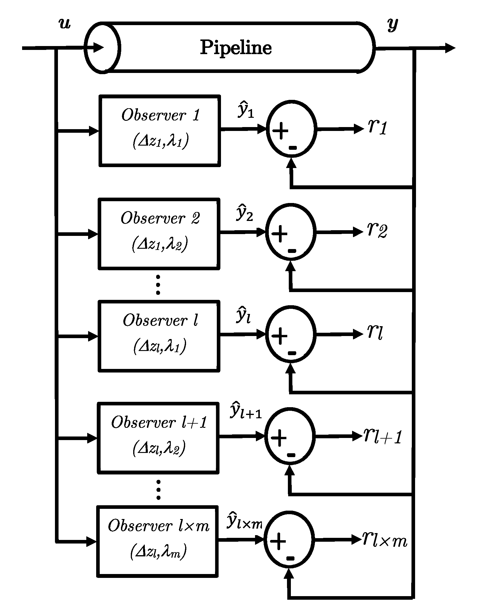
3.3. Evolutionary Ensemble of Observers

At this point, let us analyze an observer with the structure of (14), in the presence of parameter errors. First, one can consider that the leak parameters ($\lambda$ and $\Delta z$) match with real values. Then, if a parametric error appears (i.e., there is a deviation between the current $\lambda$ or $\Delta z$ and the real ones), the observer structure given by (14) changes in the following form:

$$\begin{array}{c}\hfill \dot{\widehat{x}}=(A+\delta \left(A\right))\widehat{x}-a_2\left[\begin{array}{c}0\\ \left(\frac{\lambda }{\Delta z}+\delta \left(\frac{\lambda }{\Delta z}\right)\right)\\ 0\end{array}\right]\sqrt{{\widehat{x}}_2}\\ \hfill +\left[\begin{array}{cc}\left(\frac{a_1}{\Delta z}+\delta \left(\frac{a_1}{\Delta z}\right)\right)& 0\\ 0& 0\\ 0& -\left(\frac{a_1}{L-\Delta z}+\delta \left(\frac{a_1}{L-\Delta z}\right)\right)\end{array}\right]u\\ \hfill +\xi \left(y\right)+K(y-\widehat{y})\hfill \\ \hfill \widehat{y}=C\widehat{x}\hfill \end{array}$$

(17)

where the symbol $\delta (•)$ denotes a parametric deviation from the real value. This means that $\delta \left(\lambda \right)$ is the difference of $\lambda$ as a sum error (i.e., the wrong value ${\lambda }_w$ could be separated as follows: ${\lambda }_w=\lambda +\delta \left(\lambda \right)$, where $\lambda$ is the real value). Then, (17) yields an error model in the following form:

$$\dot{e}=(A-KC)e+{\phi }^{\prime }(x,\widehat{x})+\delta \left(A\right)\widehat{x}+\left[\begin{array}{c}0\\ a_2\delta \left(\frac{\lambda }{\Delta z}\right)\\ 0\end{array}\right]\sqrt{{\widehat{x}}_2}$$

(18)

From (18), we have that

$$\delta \left(A\right)\widehat{x}+\left[\begin{array}{c}0\\ a_2\delta \left(\frac{\lambda }{\Delta z}\right)\\ 0\end{array}\right]\sqrt{\widehat{x_2}}$$

changes the equilibrium point of (15) away from 0. Thus, a residual $r\left(t\right)$ is induced in the output error $y-C\widehat{x}$ when an error presented in $\lambda$ or $\Delta z$ and this residual $r\left(t\right)$ is zero only when the $\lambda$ and $\Delta z$ match the real values. The present work exploits this system property (as long as the rest of the parameters are properly tuned). It is interesting to see that the residuals do not depend on the input signal $u\left(t\right)$.

Hence, it is possible to design an ensemble of observers, each with different values of $\lambda$ and $\Delta z$, such that the residuals of individual observers (namely, $r_1$, $r_2$,..., $r_n$) go away from zero as long as these values do not match with the real ones. Figure 4 depicts this idea.

If the residual is minimized somehow, then it is possible to estimate the correct values of the leak parameters. The present work proposes a GA that searches the correct values of $\lambda$ and $\Delta z$ by minimizing the integral squared residual of the ensemble of observers. In this GA, the population is built with the combination (cartesian product) of the possibles values of $\lambda$ and $\Delta z$. The following optimization problem is considered. Find $\left(\Delta z,\lambda \right)$ such that:

$$minimize\underset{t_0}{\overset{t_0+T}{\int }}{\left(r\left(t\right)\right)}^{2}dt$$

(19)

where the residual vector is defined as:

$$\mathbf{r}\left(t\right)=\left[\begin{array}{c}{r}_1\\ r_2\\ ⋮\\ r_n\end{array}\right]$$

(20)

Here, $r_i\left(t\right)=y\left(t\right)-{\widehat{y}}_i\left(t\right)$ is the residual of the ith observer and n is the cross product between the number of the position and magnitude that we are looking for, i.e., $n=l\times m$. Here, l and m are the number of position and magnitude, respectively, arbitrarily proposed by the designer. This work suggests to set $l=m$ such that each value of the variables $\Delta z_i$ and ${\lambda }_i$ belongs to a set of equally separated values, i.e., $\Delta z_i\in \{\Delta z_{min},2\Delta z_{min},\dots ,m\Delta z_{min}=\Delta z_{max}\}$ and ${\lambda }_i\in \{{\lambda }_{min},2{\lambda }_{min},\dots ,l{\lambda }_{min}={\lambda }_{max}\}$. Initial time $t_0$ can be deleted, as well as window length T.

4. Experimental Results

In this section, the proposed LDI methodology performance is evaluated. To ensure the method’s effectiveness, three experiments were carried out by using some database coming from the pilot plant built at Cinvestav-Guadalajara. Three different leaks were emulated by opening three electro-valves located at diverse positions along the pilot pipe.

The section continues as follows: First, a brief description of the pilot pipe is given, and then the experimental setup is stated. Finally, each experiment is described in detail.

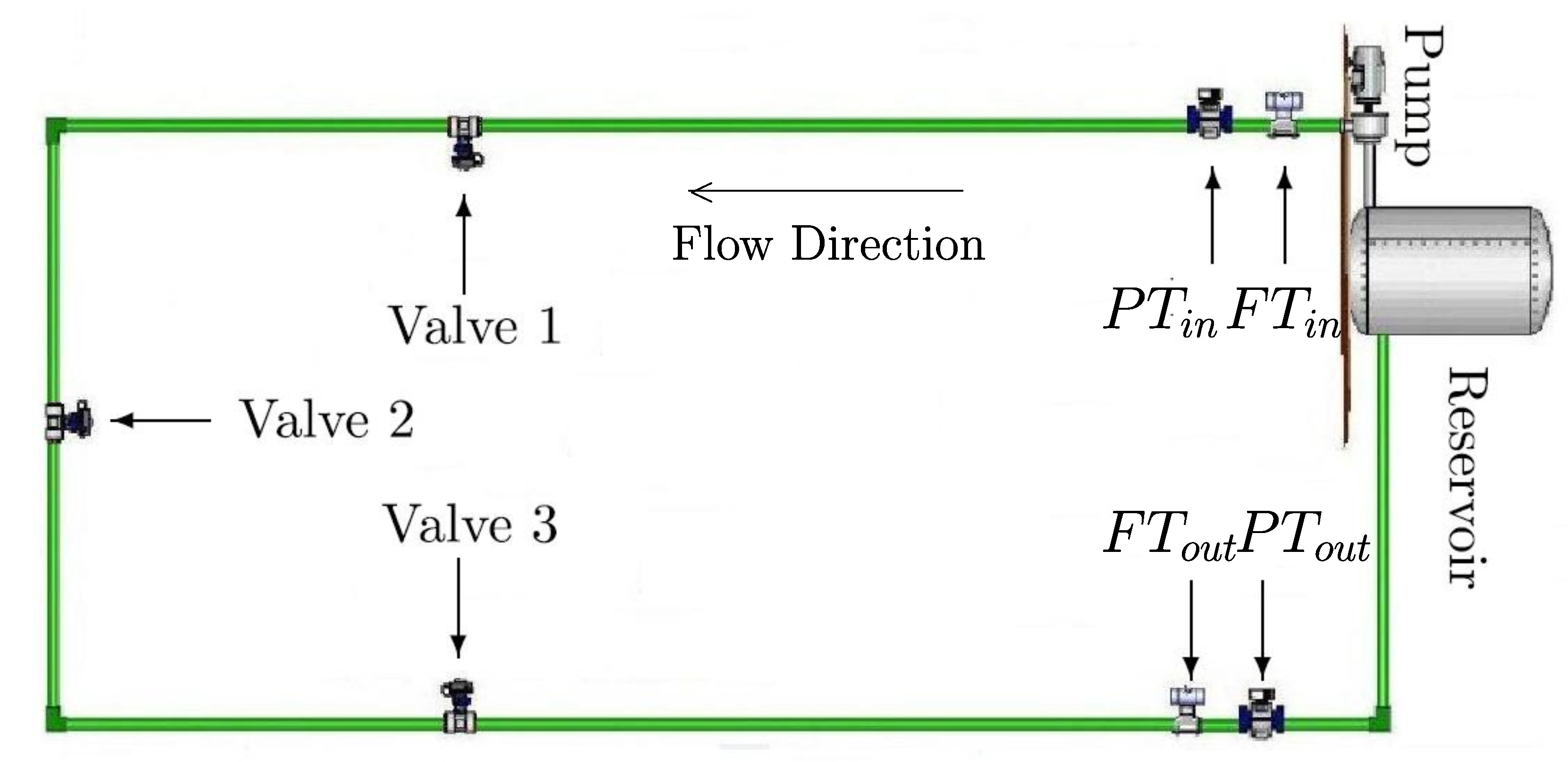
4.1. Experimental Setup

The pilot plant referred above was manufactured with PP-R (Polypropylene Copolymer Random), and it is equipped with: two flow rate transducers (FT) and two pressure-head transducers (PT) installed at both ends of the pipe. In addition, a 5 HP centrifugal pump was connected to a variable-frequency driver fixed at 50 Hz (to experiment on flow-rate variation effects over the LDI scheme); and three valves were used to emulate the leak effect. Figure 5 depicts a schematic diagram of the pipeline prototype. More information can be found in Begovich et al. [2]. The main parameters of the pipeline system are shown in

Table 1. Pipeline prototype parameters.

Parameter	Symbol	Value
Length between PT sensors	$L_r$	68.84 m
Internal diameter	$\varphi$	$6.54\times {10}^{-2}$ m
Friction factor	f	$1.635\times {10}^{-2}$
Gravity acceleration	g	9.81 m/s${}^2$
Pressure wave speed	b	341 m/s
Fitting loss coefficient sum	${\sum }_{j=i}^n{K}_j$	$9.09$ [-]

. The sampling rate was 300 Hz satisfying the Courant’s condition for system (8).

As mentioned above, the mathematical model used to derive the LDI algorithm given by (8) assumes a straight pipeline, and the prototype is not straight. Therefore, it is necessary to find an Equivalent Straight Length (ESL) for this prototype. Expression (9) is useful for this purpose (for more information, see Navarro et al. [34]).

Table 2. Distances in ESL.

Estimated in ESL Terms	Symbol	Value
Between PT sensors	L	105.1 m
Upstream to Valve 1	$z_{f1}$	30.92 m
Upstream to Valve 2	$z_{f2}$	43.64 m
Upstream to Valve 3	$z_{f3}$	62.99 m

establishes the ESL between sensors (see Figure 5) and also from upstream to each valve.

By substituting those pipeline parameters shown in Table 1 into the matrices A, $\phi \left(x\right)$, and $\varphi \left(u\right)$, $\xi \left(y\right)$ in (13), one can see that the observability matrix in (12) has full rank if $z_f\in (0,L_r)$, Torres et al. [35]. The experiments started in a free-leak condition, and at time $t_l\approx 40\left[s\right]$, a leak was induced by opening Valves 1–3, respectively. Each leak was detected once the following threshold was triggered:

$$|Q_{in}\left(t\right)-Q_{out}\left(t\right)|>\delta$$

(21)

where $\delta =1.55\times {10}^{-4}[m^3/s]$ was chosen considering the noise variance of the flow rate measurements in order to avoid false alarms. The ensemble of observers was turned on with the parameters shown in Table 1. The integration error of each residual was computed in a time-window of $T=22\left[s\right]$ in (19), where $T=t_i-t_{i-1}$, with $i\in \mathbb{N}$ and $t_0$ the time of leak occurrence. This procedure means that, once the leak was detected, executions of the GA were performed with period $T=22\left[s\right]$ (selection, crossover, and mutation). In Figures 7, 8, 10, 11, 13 and 14, this scheduled-process is indicated by: $t_1$, $t_2$, $t_3$, $t_4$, $t_5$ and $t_6$. Therefore, the integral in (19) becomes:

$$minimize\underset{t_{i-1}}{\overset{t_i}{\int }}{\left(r\left(t\right)\right)}^{2}dt$$

(22)

Notice that the selected values of the leak parameters, $\Delta z$ and $\lambda$, were held at time $t_{i-1}$ and reflected up to the next GA-process at time $t_i$.

In other words, the time-integration-window $t_i$ served for the election of $\Delta z$ and $\lambda$ used in next iteration $t_{i+1}$ and so on. In the period $t_1$, random values of $\Delta z$ and $\lambda$ were used.

The initial conditions of the observers were fixed as follows: ${\widehat{x}}_1^0={\widehat{Q}}_{in}^0$ and ${\widehat{x}}_3^0={\widehat{Q}}_{out}^0$ were equal to the mean values of the input and output flows in steady state in free-leak condition. ${\widehat{x}}_2^0={\widehat{H}}_2^0$, the pressure head at the pipeline middle point, was calculated at distance $\widehat{\Delta z}=L/2$. Finally, ${\widehat{\lambda }}_i$ (i.e., the leak magnitude of each observer) were fixed as zero, since the pipeline was not leaking.

Table 3. Initial conditions for the observer.

Estimated	Symbol	Value
${\widehat{Q}}_{in}^0$	${\widehat{x}}_1^0$	$8\times {10}^{-3}$ [m${}^3$/s]
${\widehat{H}}_2^0$	${\widehat{x}}_2^0$	12 [m]
${\widehat{Q}}_{out}^0$	${\widehat{x}}_3^0$	$8\times {10}^{-3}$ [m${}^3$/s]

summarizes those values.

To minimize the integration error in (22), the following considerations were made: the initial population vector of the algorithm was fixed by the cross product of two sets, both formed by uniformly spaced pipe sections $\Delta z_i\in \{\Delta z_{min},2\Delta z_{min},\dots ,m\Delta z_{min}=L\}$ and ${\lambda }_i\in \{{\lambda }_{min},2{\lambda }_{min},\dots ,l{\lambda }_{min}={\lambda }_{max}\}$, where $\Delta z_{min}=3.507\left[m\right]$ and ${\lambda }_{min}=6.697\times {10}^{-6}[m^{5/2}/s]$.

Remark 1.

It is worth noting that ${\lambda }_{max}$ was chosen such that the hole induces a flow through a leak $10\%$ the size of the pipeline nominal flow at most. A leak higher than this percent is considered as a failure (a catastrophic breakdown of the system’s ability to perform a required function under specified operating condition Isermann [36], and this topic goes beyond the scope of this paper).

The $SNR$ (signal-to-noise ratio) of each input and output signal is shown in

Table 4. Signal-to-noise ratio of the input and output signals.

Variable	SNR
$H_{in}$	$2.008\times {10}^1$
$H_{out}$	$6.689\times {10}^1$
$Q_{in}$	$1.338\times {10}^2$
$H_{out}$	$1.432\times {10}^2$

. The $SNR$ was calculated as the ratio of the signal power to the background noise Papoulis and Pillai [37]:

$$SNR=\frac{E\left[s^2\right]}{{\sigma }^2}$$

where $E\left[•\right]$ refers to the expected value and $\sigma$ stands for the standard deviation of the noisy signal.

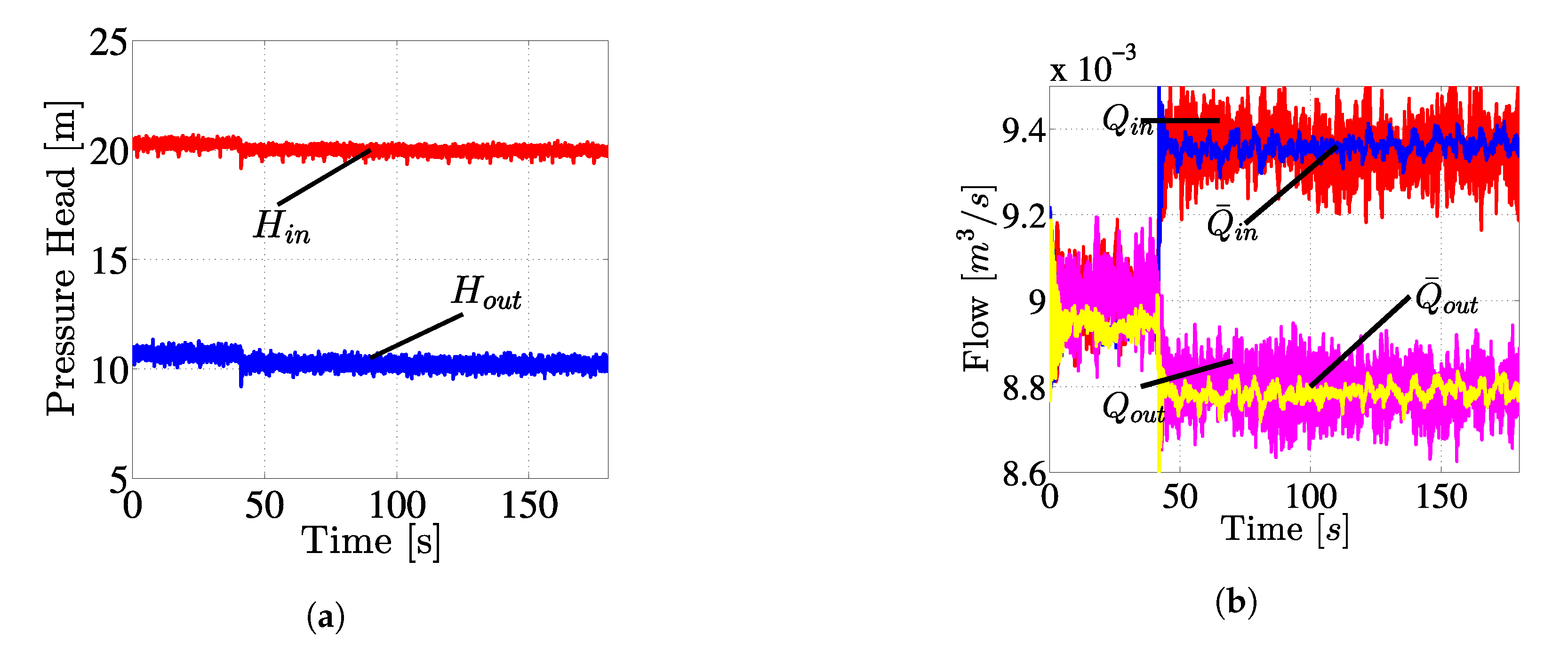
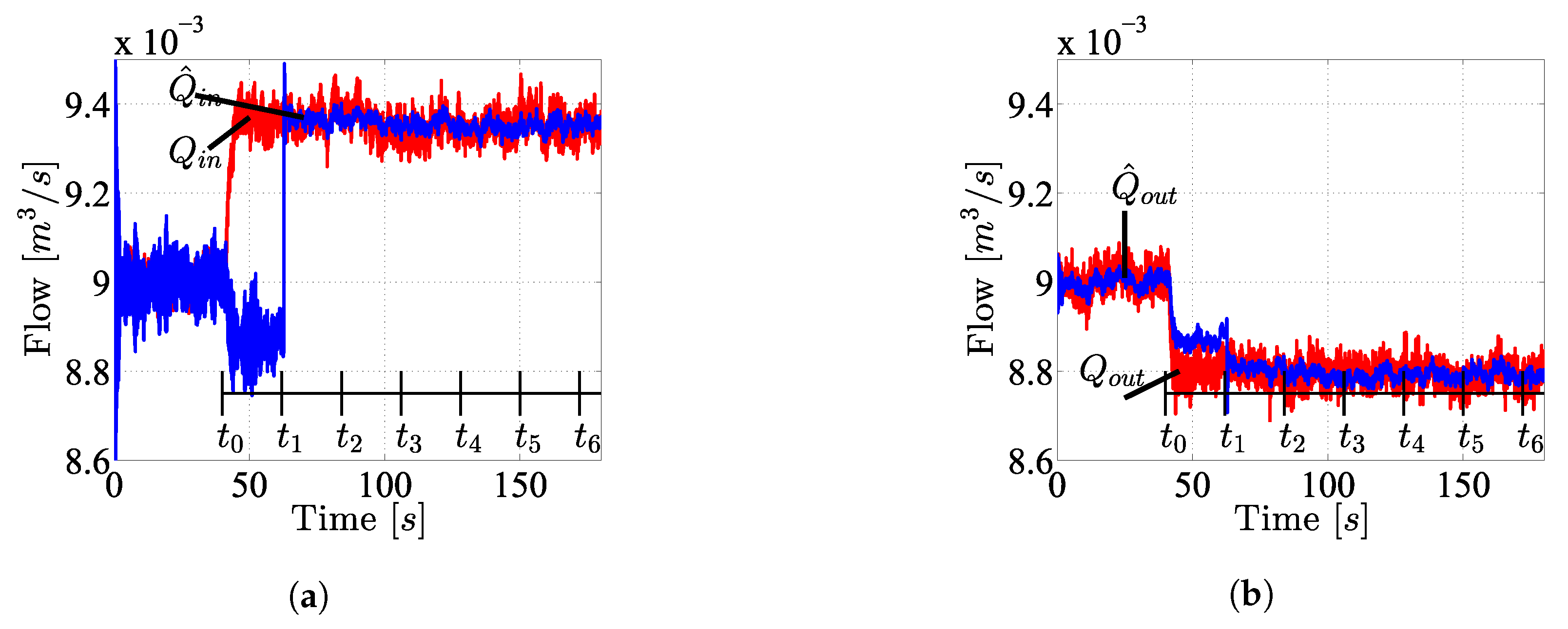
4.2. Leak Isolation Scheme Results

The proposed scheme was tested by three off-line experiments using some database. First, to ensure the validity of the mathematical model (8) in a free-leak and leak conditions, synthetic data were generated using the ESL parameters (shown in Table 2) and then were compared with their corresponding real data. Some discussions and results are described to demonstrate the Leak Isolation Scheme’s effectiveness.

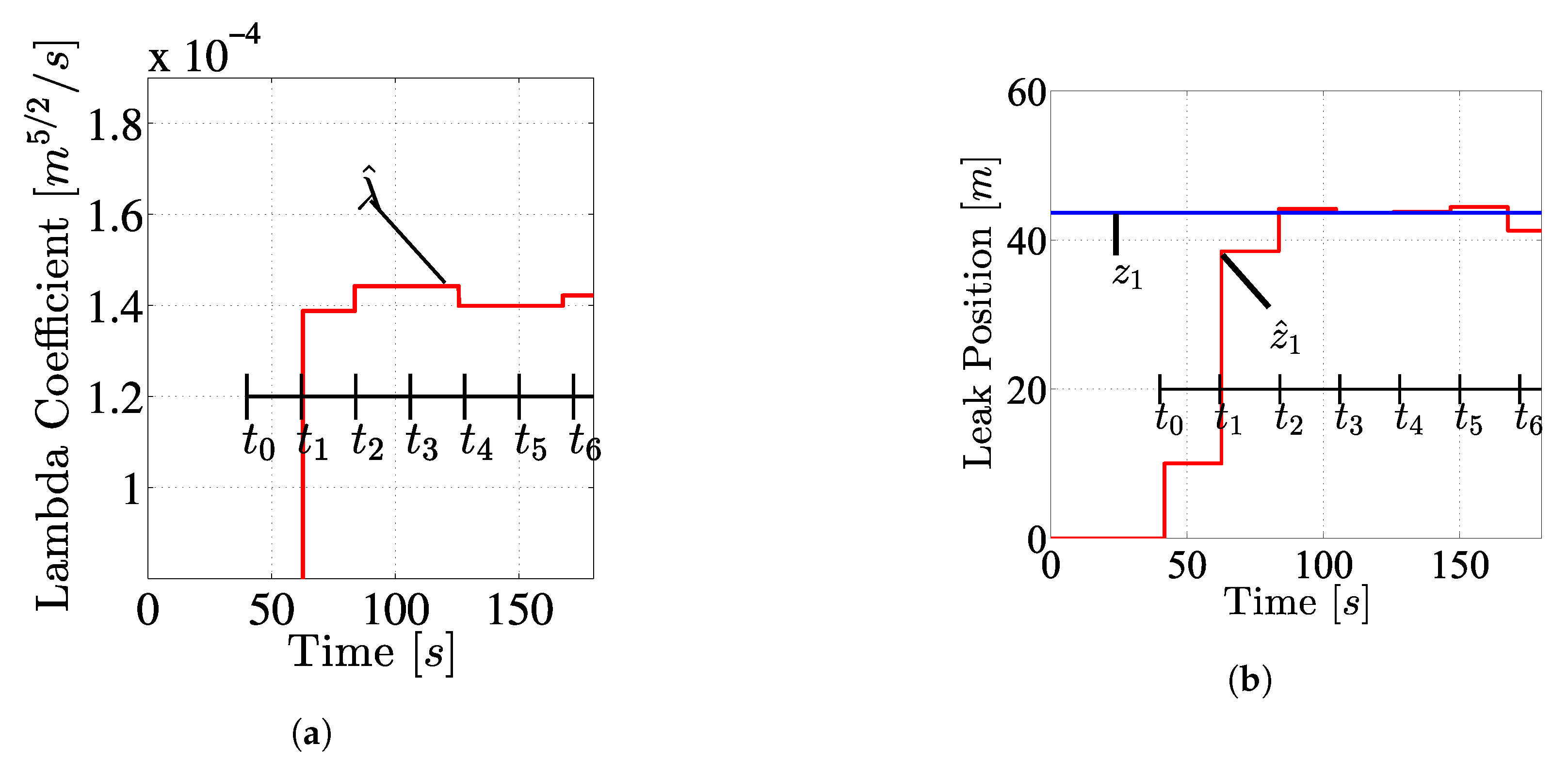
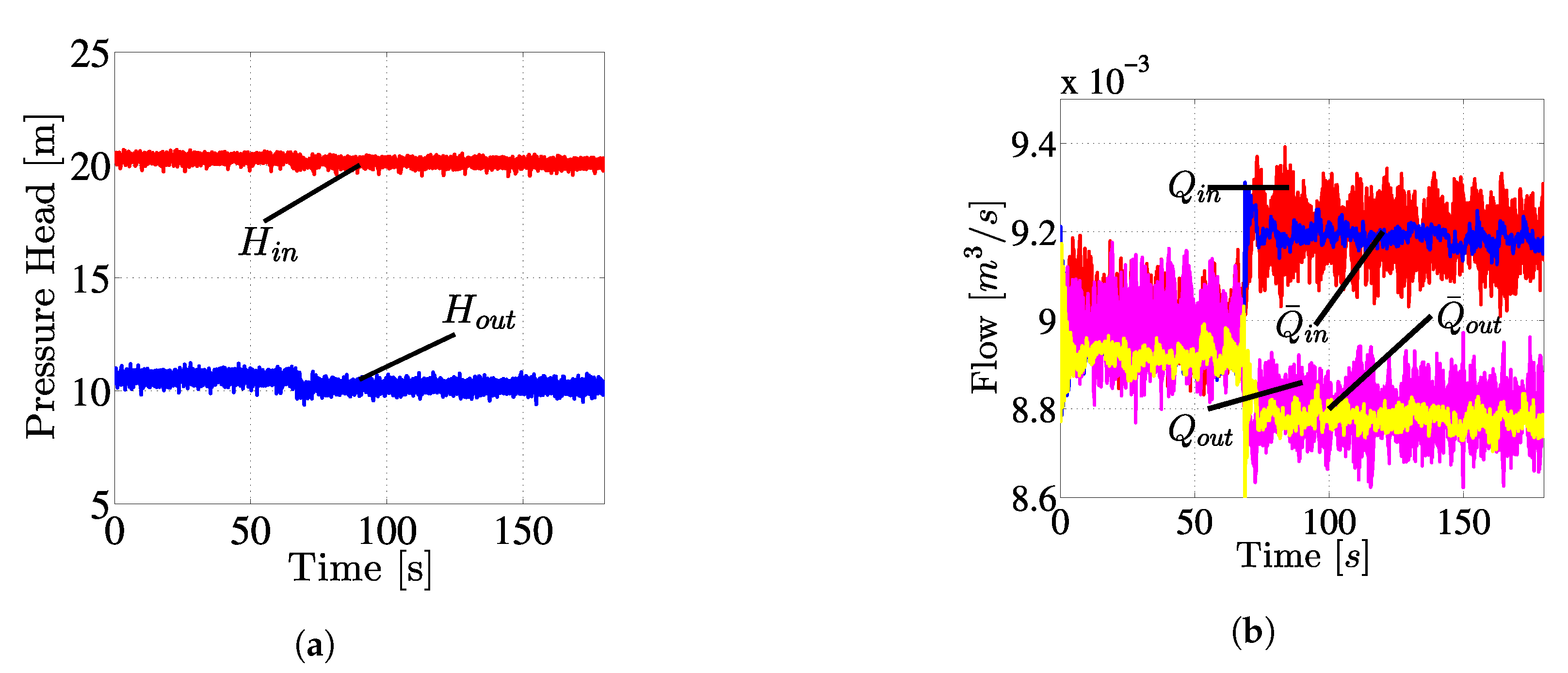
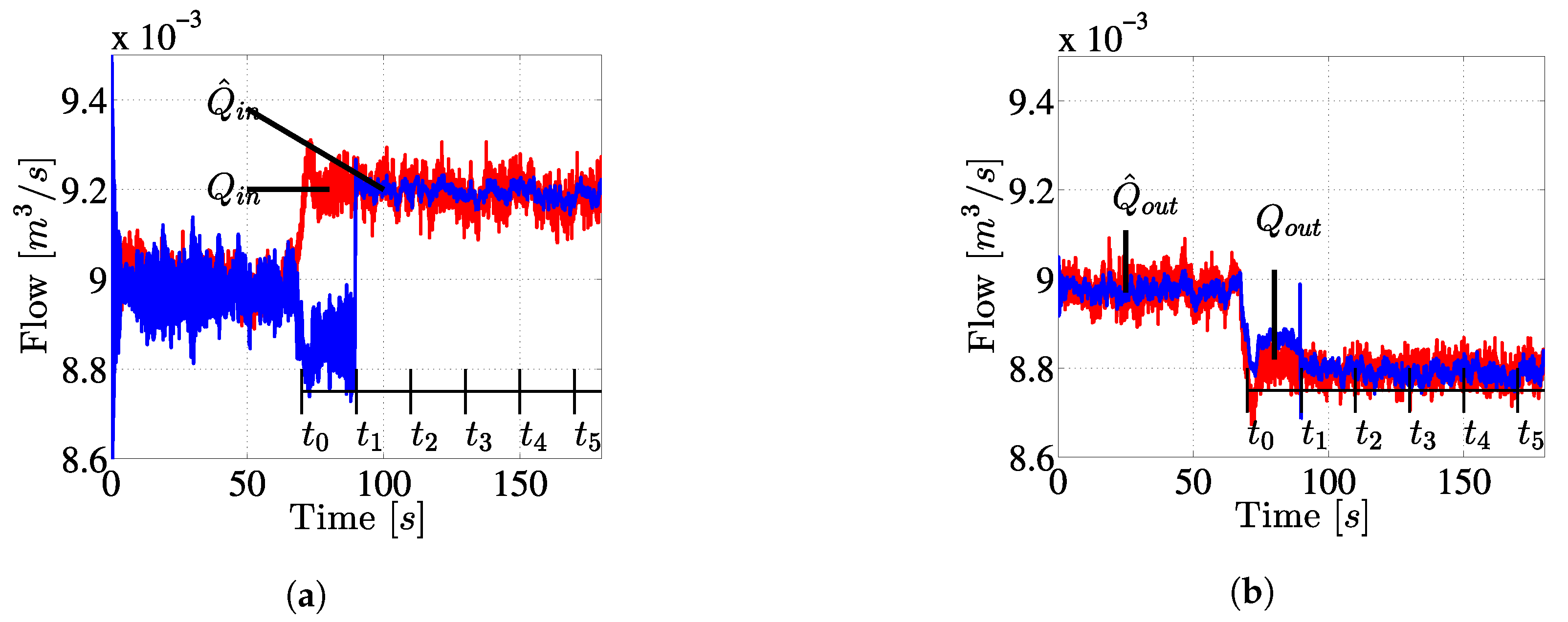
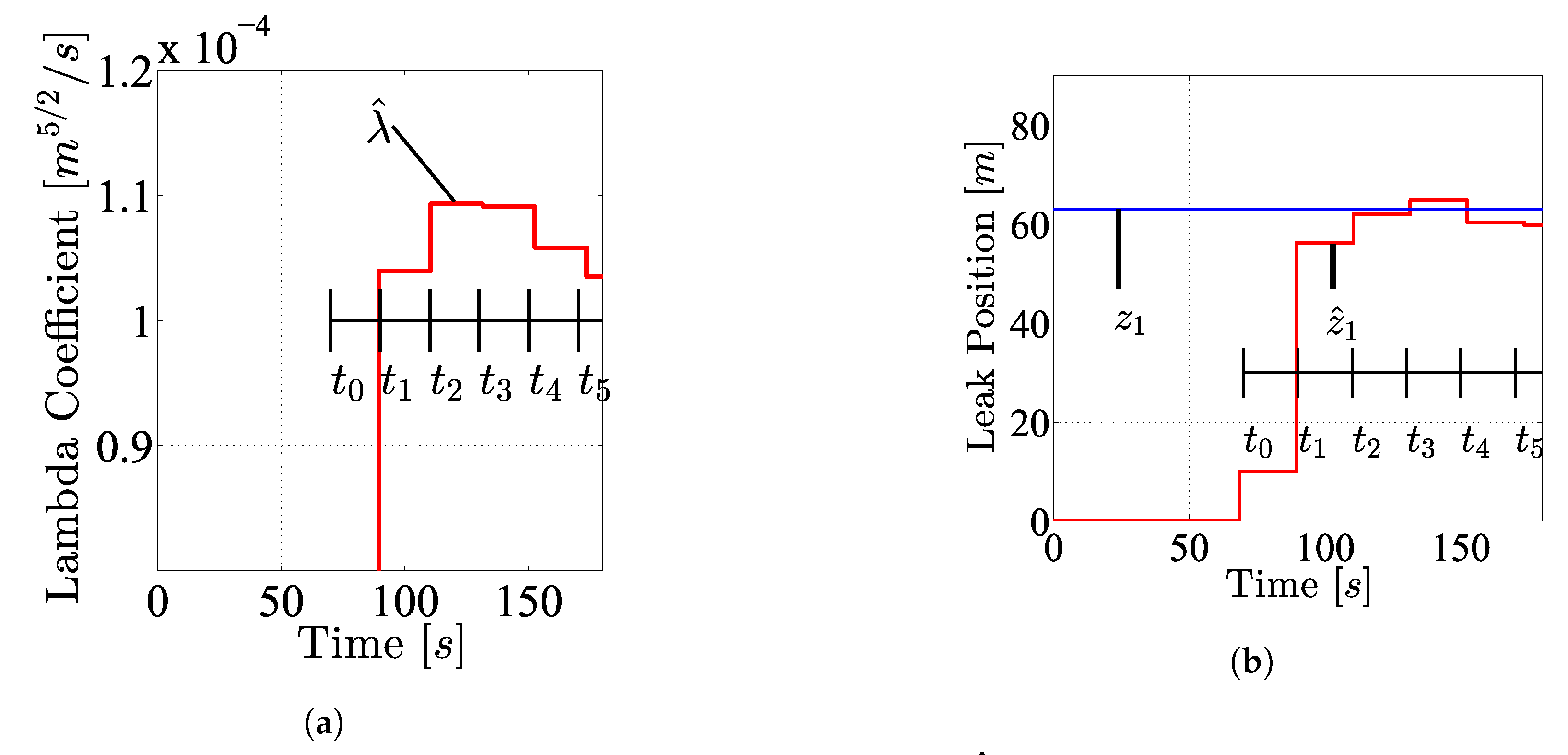
4.2.1. Leak Case in Valve 1

Initially, results in a leak induced in Valve 1 are shown. Figure 6a depicts the measured pressure head at inlet $(u_1=H_{in})$ and outlet $(u_2=H_{out})$ of the pipeline (i.e., the observation input). Figure 6b shows the measured flow upstream $(x_1=Q_{in})$ and downstream $(u_1=H_{in})$ of the pipe together with their respective synthetic data (${\overline{Q}}_{in}$ and ${\overline{Q}}_{out}$), generated by (8). As it can be seen, the mathematical model follows the real data in a proper way despite the measurement noise.

Figure 7a,b shows the evolution of the state observer: upstream and downstream flow rate, respectively. Notice that the inlet and outlet flow rate are well estimated after the first integration time, $t_1$. This fact shows that the GA chooses the appropriate values of $\Delta z$ and $\lambda$.

The results of the LDI scheme are depicted in Figure 8a,b, where the leak size and its position estimation are shown. As it can be seen, the leak position in all three cases is well estimated despite signal noise.

4.2.2. Leak Case in Valve 2

Now, results in a leak induced in Valve 2 are shown. As before, Figure 9a depicts the measured pressure head at inlet $(u_1=H_{in})$ and outlet $(u_2=H_{out})$ of the pipeline. Figure 9b shows the measured flow upstream $(x_1=Q_{in})$ and downstream $(u_1=H_{in})$ of the pipe together with their respective synthetic data (${\overline{Q}}_{in}$ and ${\overline{Q}}_{out}$). In this second case, the mathematical model follows the real data in a proper way, as well. Figure 10a,b depicts the evolution of the state observer: upstream and downstream flow rate, respectively. Figure 11a,b depicts the leak size and its position estimation.

4.2.3. Leak Case in Valve 3

Finally, the results in a leak induced in Valve 3 are shown. Figure 12a depicts the measured pressure head at inlet $(u_1=H_{in})$ and outlet $(u_2=H_{out})$ of the pipeline. Figure 12b shows the measured flow upstream $(x_1=Q_{in})$ and downstream $(u_1=H_{in})$ of the pipe together with their respective synthetic data (${\overline{Q}}_{in}$ and ${\overline{Q}}_{out}$). In the same way as before, the mathematical model follows the real data in a proper way. Figure 13a,b depicts the evolution of the state observer: upstream and downstream flow rate, respectively. Figure 14a,b depicts the leak size and its position estimation.

5. Conclusions and Future Work

The present work deals with the leak isolation problem (to estimate the position and magnitude of a leak in a water pipeline) using a heuristic method. The proposed scheme assumes only flow and pressure sensors at the upstream and downstream of the pipeline. Exploiting the fact that the pipeline mathematical model is observable, it is possible to design an observer where the observation dynamic error system is exponentially stable only if the leak size and location parameters are known and, at last, uniform ultimate boundedness in other cases. In this way, the authors propose to design a bank of observers together with a Genetic Algorithm. This scheme allows for minimizing the integral observation error. Then, the minimum integral observation error will be reached when the leak position and magnitude match the real ones.

The approach presented in the paper estimated the leak position and its intensity in a very acceptable way. This is corroborated since both downstream and upstream flow rates were well estimated in the presence of noise. It means that the genetic algorithm chooses the real values of the $\lambda$ (size of the leak) and $\Delta z$ (leak location). The use of the integration error as a fitness function helped obtain a good estimation despite the presence of noise.

As future work, this algorithm will be refined to achieve better performance. Moreover, the authors will explore the possibility of extending the present approach to two or more leaks. Finally, the algorithm will be tested to locate leaks in a hydraulic network.

References

1. CONAGUA. Sectorización en Redes de Agua Potable; Technical report; Semarnat: Mexico City, Mexico, 2007.
2. Begovich, O.; Pizano, A.; Besançon, G. Online implementation of a leak isolation algorithm in a plastic pipeline prototype. Lat. Am. Appl. Res. 2012, 57, 131–140. [Google Scholar]
3. Billman, L.; Isermann, R. Leak Detection Methods for Pipelines. Automatica 1987, 23, 381–385. [Google Scholar] [CrossRef]
4. Delgado-Aguiñaga, J.; Besançon, G.; Begovich, O.; Carvajal, J. Multi-leak diagnosis in pipelines based on Extended Kalman Filter. Control Eng. Pract. 2016, 49, 139–148. [Google Scholar] [CrossRef]
5. Verde, C.; Molina, L.; Torres, L. Parameterized transient model of a pipeline for multiple leaks location. J. Loss Prev. Process. Ind. 2014, 29, 177–185. [Google Scholar] [CrossRef]
6. Ostapkowicz, P. Leakage detection from liquid transmission pipelines using improved pressure wave technique. Eksploatacja i Niezawodność Maintenance Reliability 2014, 16, 9–16. [Google Scholar]
7. Zhang, T.; Tan, Y.; Zhang, X.; Zhao, J. A novel hybrid technique for leak detection and location in straight pipelines. J. Loss Prev. Process. Ind. 2015, 35, 157–168. [Google Scholar] [CrossRef]
8. Tian, S.; Du, J.; Shao, S.; Xu, H.; Tian, C. A study on a real-time leak detection method for pressurized liquid refrigerant pipeline based on pressure and flow rate. Appl. Therm. Eng. 2016, 95, 462–470. [Google Scholar] [CrossRef]
9. Santos-Ruiz, I.; Bermúdez, J.; López-Estrada, F.; Puig, V.; Torres, L.; Delgado-Aguiñaga, J. Online leak diagnosis in pipelines using an EKF-based and steady-state mixed approach. Control Eng. Pract. 2018, 81, 55–64. [Google Scholar] [CrossRef]
10. Delgado-Aguiñaga, J.A.; Begovich, O. Water Leak Diagnosis in Pressurized Pipelines: A Real Case Study. In Modeling and Monitoring of Pipelines and Networks; Verde, C., Torres, L., Eds.; Springer International Publishing: Cham, Switzerland, 2017; Volume 7, pp. 235–262. [Google Scholar] [CrossRef]
11. Liu, C.; Li, Y.; Fang, L.; Xu, M. New leak-localization approaches for gas pipelines using acoustic waves. Measurement 2019, 134, 54–65. [Google Scholar] [CrossRef]
12. Rubio Scola, I.; Besancon, G.; Georges, D.; Guillén, M.; Dulhoste, J.F.; Santos, R. On the design of a nonlinear state observer for the location of a blockage in a pipeline. In Proceedings of the XII International Congress on Numerical Methods in Engineering and Applied Sciences, Pampatar, Magarita Island, Venezuela, 24–26 March 2014. [Google Scholar]
13. Lyu, P.; Liu, S.; Lai, J.; Liu, J. An analytical fault diagnosis method for yaw estimation of quadrotors. Control Eng. Pract. 2019, 86, 118–128. [Google Scholar] [CrossRef]
14. Chouchane, A.; Khedher, A.; Nasri, O.; Kamoun, A. Diagnosis of Partially Observed Petri Net Based on Analytical Redundancy Relationships. Asian J. Control 2019. [Google Scholar] [CrossRef]
15. Lunze, J. A method to get analytical redundancy relations for fault diagnosis. IFAC-PapersOnLine 2017, 50, 1006–1012. [Google Scholar] [CrossRef]
16. Witczak, M. Advances in model-based fault diagnosis with evolutionary algorithms and neural networks. Int. J. Appl. Math. Comput. Sci. 2006, 16, 85–99. [Google Scholar]
17. Vitkovsky, J.P.; Simpson, A.R.; Lambert, M.F. Leak Detection and Calibration Using Transients and Genetic Algorithms. J. Water Resour. Plan. Manag. 2000, 126, 262–265. [Google Scholar] [CrossRef] [Green Version]
18. Wu, Z.Y.; Sage, P. Water Loss Detection via Genetic Algorithm Optimization-based Model Calibration. In Proceedings of the Water Distribution Systems Analysis Symposium 2006, Cincinnati, OH, USA, 27–30 August 2006; pp. 1–11. [Google Scholar] [CrossRef] [Green Version]
19. Roberson, J.A.; Cassidy, J.J.; Chaudhry, M.H. Hydraulic Engineering; Wiley: Hoboken, NJ, USA, 1998. [Google Scholar]
20. Delgado-Aguiñaga, J.; Begovich, O.; Besançon, G. Exact-differentiation-based leak detection and isolation in a plastic pipeline under temperature variations. J. Process. Control 2016, 42, 114–124. [Google Scholar] [CrossRef]
21. Navarro, A.; Begovich, O.; Sánchez Torres, J.D.; Besancon, G. Real-Time Leak Isolation Based on State Estimation with Fitting Loss Coefficient Calibration in a Plastic Pipeline: Real-Time Leak Isolation based on State Estimation. Asian J. Control 2016. [Google Scholar] [CrossRef]
22. Brkić, D. Review of explicit approximations to the Colebrook relation for flow friction. J. Pet. Sci. Eng. 2011, 77, 34–48. [Google Scholar] [CrossRef] [Green Version]
23. Swamee, P.K.; Jain, A.K. Explicit equations for pipe-flow problems. J. Hydraul. Div. 1976, 102, 657–664. [Google Scholar]
24. Verde, C. Accommodation of multi-leak location in a pipeline. Control Eng. Pract. 2005, 13, 1071–1078. [Google Scholar] [CrossRef]
25. Besançon, G.; Georges, D.; Begovich, O.; Verde, C.; Aldana, C. Direct observer design for leak detection and estimation in pipelines. In Proceedings of the European Control Conference, ECC’07, Kos, Greece, 2–5 July 2007; pp. 5666–5670. [Google Scholar]
26. Mott, R.L. Applied Fluid Mechanics, 6th ed.; Prentice-Hall: Upper Saddle River, NJ, USA, 2006. [Google Scholar]
27. Birk, J.; Zeitz, M. Extended Luenberger observer for non-linear multivariable systems. Int. J. Control 1988, 47, 1823–1836. [Google Scholar] [CrossRef]
28. Krener, A.J.; Isidori, A. Linearization by output injection and nonlinear observers. Syst. Control Lett. 1983, 3, 47–52. [Google Scholar] [CrossRef]
29. J. Krener, A.; Respondek, W. Nonlinear Observer with Linearizable Error Dynamics. SIAM J. Control Optim. 1985, 23. [Google Scholar] [CrossRef]
30. Khalil, H.K. Nonlinear Systems, 2nd ed.; Prentice-Hall: Upper Saddle River, NJ, USA, 1996. [Google Scholar]
31. Schmitt, L.M. Theory of Genetic Algorithms. Theor. Comput. Sci. 2001, 259, 1–61. [Google Scholar] [CrossRef] [Green Version]
32. Mitchell, M. An Introduction to Genetic Algorithms; MIT Press: Cambridge, MA, USA, 1998. [Google Scholar]
33. Whitley, D. A genetic algorithm tutorial. Stat. Comput. 1994, 4, 65–85. [Google Scholar] [CrossRef]
34. Navarro, A.; Begovich, O.; Besançon, G.; Dulhoste, J. Real-time leak isolation based on state estimation in a plastic pipeline. In Proceedings of the IEEE International Conference on Control Applications (CCA), Denver, CO, USA, 28–30 September 2011; pp. 953–957. [Google Scholar] [CrossRef]
35. Torres, L.; Besançon, G.; Georges, D.; Navarro, A.; Begovich, O. Examples of pipeline monitoring with nonlinear observers and real-data validation. In Proceedings of the 8th International Multi-Conference on Systems, Signals and Devices, Sousse, Tunisia, 22–25 March 2011. [Google Scholar]
36. Isermann, R. Fault Diagnosis Systems an Introduction from Fault Detection to Fault Tolerance; Springer: Heidelberg/Berlin, Germany, 2006. [Google Scholar]
37. Papoulis, A.; Pillai, S.U. Probability, Random Variables, and Stochastic Processes, 4th ed.; McGraw Hill: Boston, MA, USA, 2002. [Google Scholar]
Figure 1. Discretization of the pipeline with a leak Q l .
Processes 07 00913 g001
Figure 2. Moody chart.
Processes 07 00913 g002
Figure 3. Genetic algorithm block diagram.
Processes 07 00913 g003
Figure 4. Evolutionary ensemble of observer block diagram.
Processes 07 00913 g004
Figure 5. Schematic diagram of the pipeline prototype.
Processes 07 00913 g005
Figure 6. Model validation for a leak induced in Valve 1: (a) pressure head at inlet an outlet of the pipeline u = [ u 1 u 2 ] T = [ H i n H o u t ] T (input signals); and (b) synthetic and real flow rates at inlet ( Q ¯ i n and Q i n ) and outlet ( Q ¯ o u t and Q o u t ) of the pipe.
Processes 07 00913 g006
Figure 7. Flow rate estimations at the ends of the pipeline: (a) flow rate at inlet of the pipe ( Q i n ) and its estimation ( Q ^ i n ); and (b) flow rate at outlet of the pipe ( Q o u t ) and its estimation ( Q ^ o u t ).
Processes 07 00913 g007
Figure 8. Leak parameters: (a) lambda parameter estimation λ ^ concerning Valve 1 (leak magnitude); and (b) leak position estimation Δ z concerning Valve 1.
Processes 07 00913 g008
Figure 9. Model validation for a leak induced in Valve 2: (a) pressure head at inlet an outlet of the pipeline u = [ u 1 u 2 ] T = [ H i n H o u t ] T (input signals); and (b) synthetic and real flow rates at inlet ( Q ¯ i n and Q i n ) and outlet ( Q ¯ o u t and Q o u t ) of the pipe.
Processes 07 00913 g009
Figure 10. Flow rate estimations at the ends of the pipeline: (a) flow rate at inlet of the pipe ( Q i n ) and its estimation ( Q ^ i n ); and (b) flow rate at outlet of the pipe ( Q o u t ) and its estimation ( Q ^ o u t ).
Processes 07 00913 g010
Figure 11. Leak parameters: (a) lambda parameter estimation λ ^ concerning Valve 2 (leak magnitude); and (b) leak position estimation Δ z concerning Valve 2.
Processes 07 00913 g011
Figure 12. Model validation for a leak induced in Valve 3: (a) pressure head at inlet an outlet of the pipeline u = [ u 1 u 2 ] T = [ H i n H o u t ] T (input signals); and (b) synthetic and real flow rates at inlet ( Q ¯ i n and Q i n ) and outlet ( Q ¯ o u t and Q o u t ) of the pipe.
Processes 07 00913 g012
Figure 13. Flow rate estimations at the ends of the pipeline: (a) flow rate at inlet of the pipe ( Q i n ) and its estimation ( Q ^ i n ); and (b) flow rate at outlet of the pipe ( Q o u t ) and its estimation ( Q ^ o u t ).
Processes 07 00913 g013
Figure 14. Leak parameters: (a) lambda parameter estimation λ ^ concerning Valve 3 (leak magnitude); and (b) leak position estimation Δ z concerning Valve 3.
Processes 07 00913 g014