Generalized Proportional Model of Relay Protection Based on Adaptive Homotopy Algorithm Transient Stability

Abstract

Relay protection equipment is important to ensure the safe and stable operation of power systems. The risks should be evaluated, which are caused by the failure of relay protection. At present, the fault data and the fault status monitoring information are used to evaluate the failure risks of relay protection. However, there is a lack of attention to the information value of monitoring information in the normal operation condition. In order to comprehensively improve monitoring information accuracy and reduce, a generalized proportional hazard model (GPHM) is established to fully exploit the whole monitoring condition information during the whole operation process, not just the monitoring fault condition data, with the maximum likelihood estimation (MLE) used to estimate the parameters of the GPHM. For solving the nonlinear equation in the process of parameter estimations, the adaptive homotopy algorithm is adopted, which could ensure the reversibility of the Jacobi matrix. Three testing cases have been reviewed, to demonstrate that the adaptive homotopy algorithm is better than traditional algorithms, such as the Newton homotopy algorithm, regarding the calculation speed and convergence. Therefore, GPHM could not only reflect the real time state of the equipment, but also provide a sound theoretical basis for the selection of equipment maintenance types.

1. Introduction

Because a relay protection device can curb the deterioration of a power grid by its fast and correct action [1], it is always seen as the first line of defense to ensure the safe and stable operation of power systems. In recent years, there have been frequent blackouts around the world, and most of them are related to the incorrect action of relay protection. Therefore, evaluation of the reliability of relay protection is the focus of many scholars, and the relay protection failure rate is one of the indexes to estimate its reliability [2,3].

At present, the research on the failure rate model is generally based on the time-failure rate model and equipment state model [4]. The commonly used fault distribution forms for the time-failure rate model are gamma distribution, Weibull distribution, and exponential distribution [5]. The failure rate of exponential distribution is constant and it only represents the accidental failure period. However, the failure rates of most electrical equipment follow the typical curve, namely the bathtub curve, and the bathtub curve includes the early failure period, the accidental failure period, and the three stages of loss failure period. Therefore, the exponential distribution generally is not adopted. By contrast, the Weibull distribution can match the bathtub curve well, so that it has been widely used. Nevertheless, the Weibull distribution only pays attention to the effect of equipment running enlistment age on the failure rate, which ignores the effect of some external factors such as the equipment maintenance on the equipment failure rate [6]. Accordingly, Weibull distribution has some limitations. The equipment state model is established based on the current state of the equipment [7], so that it does not take the effects of man-made maintenance and historical condition on the failure rate into account, and so it is difficult to predict the future failure rate. Furthermore, there are differences between countries/power companies. The British EA company and Canada Kinectrics Company focus on the health state [8,9]. In China, the failure rate model is an exponential function, which considers the health state as the independent variable [10,11,12], and from the model, the failure rate may increase exponentially when the equipment state worsens, and the failure rate is beyond 1, so that it doesn’t conform to the actual situation. In other words, it is difficult to predict the future failure rate. Aiming at the shortcoming of the two kinds of failure rate model, a Weibull proportional hazards model (PHM), which considered the fault diagnosis value of failure time and used maximum likelihood estimation (MLE) to estimate the model parameters, has been proposed in [13]. In [14], the proportional covariate model (PCM) was put forward in order to solve the lack of data in the fault interval. For a repairable system, the proportional intensity model (PIM) were first proposed by Kumar [15]. Kumar said that the fault rate in a repairable system was affected by many factors, such as operating environment, equipment materials, history operation, design features, and so on. However, the PIM always assumed that the covariates were changed only when failure/maintenance occurred, and maintained constant during the interval of failure/maintenance [16,17]. This assumption ignored the influence of the concomitant variables on the failure rate during the failure/maintenance interval. In [18], the PHM was used to estimate the reliability of thin oxide dielectrics, and used the partial maximum likelihood method to estimate the parameters. In [19], the scholars pointed out that the environmental factors influencing relay reliability mainly included temperature, humidity, vibration, and so on. Additionally, the application of Cox-proportional hazards modeling with respect to the effect of ambient temperature on electromagnetic relays was discussed.

For the above model, ignoring the whole monitoring condition values is the common point. Therefore, based on the above model, this paper analyzes the influence of variables during the failure/maintenance interval, and takes the time varying covariates in the failure/maintenance interval into account, not only the monitoring state value at failure time; then, the generalized proportional hazards model (GPHM) Weibull is built. In order to get the expressions of fault rate, the parameters of Weibull distribution are needed to estimate, which involves the solution for nonlinear equations. At present, there are many the solutions for nonlinear equations, such as the Newton method, the least square method [20], the Marquardt method [21], and so on. There are also many achievements on the solution of nonlinear equations, whereas they still have a fatal defect, namely, local convergence [22]. Because the initial value must be close to the exact one, the requirement of the initial value is very harsh. In the meantime, the calculation is a large amount which brings certain challenges to the running time and space. Actually, for many nonlinear equations, the initial value is not easy to set, which brings inconvenience to the solution of nonlinear equations. Fortunately, the homotopy algorithm has a large convergence range and its requirement on the initial value is not strict, so that it brings a breakthrough to solve nonlinear equations [23]. Howver, the Jacobi matrix of the homotopy algorithm must be reversible, otherwise the homotopy algorithm loses its significance [24]. For solving this problem, the adjusting factor is introduced to construct an adaptive homotopy algorithm to ensure the non-singularity of the Jacobi matrix in this paper. Then, the nonlinear equation can be solved. In summary, in order to fully consider the influence of time–varying covariates in the failure/maintenance interval on the failure rate, the GPHM-Weibull is proposed, which can reflect the real-time state. MLE is used to estimate parameters of GPHM, and the adaptive homotopy algorithm is used to solve nonlinear equation, where the piecewise function expression of fault rate is solved. According to the failure rate, the operation personnel can make the differential operation strategy and realize the economic, stable operation of the power system.

Section 2 presents the generalized proportional hazard model. Section 3 describes the adaptive homotopy algorithm. Section 4 discusses the estimation of Weibull distribution parameters, the solution of nonlinear equations and the calculation of the initial value. Section 5 presents a summary of the proposed method and draws relevant conclusions.

2. Generalized Proportional Hazard Model

With reference to survival function model in medical science [25], based on GPHM, the failure rate model is constructed, and its mathematical expression is as follows:

$$\lambda (t|Z)={\lambda }_0(t)\psi (Z(t))$$

(1)

Here, λ₀(t) is the basic failure rate. Ψ(Z(t)) is the link function, representing the impact of different states Z(t) on failure rate. Z(t) is a vector of covariates, which is composed of n time-varying covariates. Each covariate can represent a particular state. The expression is Z(t) = [Z₁(t), Z₂(t) … Z_n(t)]. In practice, the covariate could be an internal variable which can reflect the state of the device, such as the detection information of device. It can also be an external variable which can affect the operation of the device, such as the environmental conditions. In general, the link function can be expressed as follows:

$$\psi \left(Z\left(t\right)\right)=exp({\gamma }_1{Z}_1\left(t\right)+{\gamma }_2{Z}_2\left(t\right)+\cdots +{\gamma }_n{Z}_n\left(t\right))$$

(2)

Here, γ = (γ₁, γ₂ … γ_n) represents the corresponding regression coefficient of each covariate. The assumptions of GPHM are as follows:

(1) The basic failure rate λ₀ (t) subjects to Weibull distribution, and its expression is

$${\lambda }_0(t)=\frac{\beta }{\eta }{(\frac{t}{\eta })}^{\beta -1}.$$

(3)

Here, β is the shape parameter, and η is the scale parameter.

(2) The fault interval is longer than maintenance time, so that the maintenance time can be neglected.

(3) The effect of covariates on the failure rate maintain constant and it cannot be changed with time.

Choosing the best covariates is the key to establish the GPHM. Age, operating environment, maintenance times, health index, and manufacturer are selected as covariates, as shown in Figure 1 [25].

Health index (HI) reflects the overall health level of the relay protection equipment, which is closely related to the equipment failure rate. In order to facilitate quantitative comparison, HI is divided into five levels (normal, attention, serious, emergency, and fault), and their corresponding values are listed in

Table 1. Values of Health Index (HI).

Grade	Normal	Attention	Emergency	Serious	Fault
values of HI	0	0.1	0.3	0.6	1

.

In [26], research’s results indicated that when the equipment is in the loss period, the failure rate meets Weibull distribution, and Weibull distribution is a function of time. It means that the failure rate is related to age. In [27], the scholars pointed out that the failure rate function directly is multiplied by the age reduction factor, and failure rate increase factor after repairmen. Because the age reduction factor and failure rate increase factor are related to the maintenance type and maintenance times, the failure rate λ_k+1(t) after kth maintenance is defined recursively as:

$${\lambda }_{k+1}(t)={\beta }_k{\lambda }_k(t+{\alpha }_k{T}_k)$$

(4)

Here, k is the kth maintenance. T_k represents the interval for the kth maintenance. β_k is age reduction factor, which can simulate the equipment damage caused by each maintenance. α_k is failure rate increase factor, which can describe the degree of improvement in equipment failure rate after maintenance.

According to [28], the failure rate can be affected the operating environment. Therefore, the business district and the industrial area differ considerably. Different manufacturers may have different familial defects which may affect the history data. With reference to [27], the values of the operating environment and manufacturers are given as

Table 2. Values of operating environment.

Operating Environment	Business District	Industrial Area
value	1	2

and

Table 3. Of the manufacturer.

Manufacturer	NR Electronic	Beijing Sifang	Changyuan Shenrui	Guodian Nanzi	Xuji Dianqi
value	1	2	3	4	5

shown.

Therefore, the expression of the failure rate $\lambda (t|Z)$ which takes the influence of covariates into consideration can be expressed as

$$\begin{array}{ll}\lambda (t|Z)=& \frac{\beta }{\eta }{(\frac{t}{\eta })}^{\beta -1}\exp ({\gamma }_{pm}{Z}_{pm}(t)+{\gamma }_{cm}{Z}_{cm}(t)+{\gamma }_{age}{Z}_{age}(t)\\ & +{\gamma }_{env}{Z}_{env}(t)+{\gamma }_{HI}{Z}_{HI}(t)+{\gamma }_{mau}{Z}_{mau}(t))\end{array}$$

(5)

Here, covariant Z_pm, Z_cm, Z_age, Z_env, Z_HI, and Z_mau respectively represent the times of preventive maintenance and corrective maintenance, age, the operating environment, the HI of equipment and manufacturer; the corresponding coefficient of the covariates are λ_pm, λ_cm, λ_age, λ_env, λ_HI, and λ_mau. Equation (5) illustrates that if you want to get to the expression of failure rate, β/η/γ_i is needed in order to estimate. The maximum likelihood function (MLE) and the adaptive homotopy algorithm are used to solve the nonlinear equations.

3. Adaptive Homotopy Algorithm

3.1. The Basicprinciple of Homotopy Algorithm

Considering the following nonlinear Equation (6):

$$\{\begin{array}{c}{f}_1(x_1,x_2,x_3,x_4\dots \dots ,x_n)=0\\ f_2(x_1,x_2,x_3,x_4\dots \dots ,x_n)=0\\ ⋮\\ f_n(x_1,x_2,x_3,x_4\dots \dots ,x_n)=0\end{array}$$

(6)

Here, x = (x₁, x₂, x₃, x₄ … x_n) ∈ Rⁿ can be obtained. f_i(x₁, x₂, x₃, x₄ … x_n) is a real function defined on a regional D, i = (1, 2, 3 … n). Its vector notation is:

$$\overrightarrow{F}(x)=\left[\begin{array}{c}{f}_1(x)\\ f_2(x)\\ ⋮\\ f_n(x)\end{array}\right]\overrightarrow{x}=\left[\begin{array}{c}{x}_1\\ x_2\\ ⋮\\ x_n\end{array}\right]\in R^n\overrightarrow{0}=\left[\begin{array}{c}0\\ 0\\ ⋮\\ 0\end{array}\right]$$

(7)

Then, Equation (7) can be converted to:

$$\overrightarrow{F}(x)=\overrightarrow{0}$$

(8)

In Equation (8), parameter t is introduced to construct a set of homotopy mapping H(x, t) which subjects to:

$$\{\begin{array}{l}H(x,0)=G(x_0)=0\\ H(x,1)=F(x)+(t-1)G(x)\end{array}$$

(9)

From Equation (9), the equations can be obtained, which are t = 0, H(x, 0) = G(x₀) and t = 1, H(x, 1) = F(x). Then, the solution of equation F(x) = 0 is transformed into the solution of equation x = x (t) which subjects to equation H(x, 1) = 0. Equation (9) indicates that due to different G(x), there are different homotopy equations.

A Fixed Point Homotopy Algorithm

If G(x) = x − x₀, then a fixed point homotopy algorithm is formed as:

$$H(x,t)=F(x)+(t-1)(x-x_0)$$

(10)

Newton Homotopy Algorithm

If G(x) = F(x) − F(x₀), then a Newton homotopy algorithm is formed as:

$$H(x,t)=tF(x)+(1-t)(F(x)-F(x_0))$$

(11)

The derivative of parameter t in H(x, t) = 0 is:

$$\frac{\partial H}{\partial x}\frac{dx}{dt}+\frac{\partial H}{\partial t}=0$$

(12)

If the inverse matrix ${(\frac{\partial H}{\partial x})}^{-1}$ exists, then:

$$\frac{dx}{dt}=-{(\frac{\partial H}{\partial x})}^{-1}.\frac{\partial H}{\partial t}$$

(13)

Adaptive Homotopy Equation

However, when inverse matrix ${(\partial H/\partial x)}^{-1}$ doesn’t exist, the homotopy algorithm will lose its significance. Because the diagonal factor $G(x)=diag[e^{g_i(x)}]$ in the exponential homotopy method is multiplied by F to construct a new homotopy algorithm, it is only feasible in theory, and the calculation is complicated and not suitable for the large-scale nonlinear equation. However, in reference to the idea of exponential homotopy algorithm, the equation for adaptive homotopy algorithm can be obtained as:

$$H(x,t)=F(x)-(1-t)[F(x_0)-a(1+t)(x-x_0)]$$

(14)

$${(\frac{\partial H}{\partial x})}^{-1}={[F^{\prime }(x)+a(1-t^2)I]}^{-1}$$

(15)

Because a (1 − t²) I is a nonsingular matrix and when ${(\partial H/\partial x)}^{-1}$ is singular, through adjusting the parameter a, it can account for the diagonal dominance, as long as a is large enough. In the actual calculation, the initial value of parameter a is set as 0. When the Jacobi matrix F′(x) becomes singular after some calculation steps, a automatic increase Δa. Thus, the solution of the Equation (7) can be obtained by finding the solution of the homotopy Equation (9).

3.2. Numerical Calculation of the Adaptive Homotopy Algorithm

Equation (13) presents that the calculation of nonlinear equations can be converted into the calculation of IVP (initial value problem), which can be expressed as:

$$\{\begin{array}{l}\frac{dx}{dt}=-{(\frac{\partial H}{\partial x})}^{-1}.\frac{\partial H}{\partial t}={[F^{\prime }(x)+a(1-t^2)I]}^{-1}.\frac{\partial H}{\partial t}\\ x_0=x(0)\end{array}$$

(16)

In order to solve the Equation (16), the Euler method is used to estimate, and the Runge Kutta method is used to correct.

Euler method

We begin to track the path from the starting point (t₀, x₀) of the homotopy path, and the Euler method is adopted to estimate the next approximate point (t₁, ${\tilde{x}}_1$), so that the expression is:

$${\tilde{x}}_1=x_0+\frac{dx}{dt}\Delta t=x_0-{(\frac{\partial H}{\partial x_0})}^{-1}\frac{\partial H}{\partial t_0}\Delta t$$

(17)

With the iterative equation as:

$$\{\begin{array}{l}{\tilde{x}}_n=x_{n-1}-{(\frac{\partial H}{\partial x_{n-1}})}^{-1}\frac{\partial H}{\partial t_{n-1}}\Delta t\\ t_{n-1}=t_1+(n-1)\times h\\ h=\frac{1}{N}\end{array}$$

(18)

Here, h is the step size, and n is the number of iterations.

The Fouth Runge Kutta method

Through using the Runge Kutta method, the local truncation error of the fourth Runge Kutta method is about o (h5) [13], and its calculation speed is fast. Therefore, the fouth Runge Kutta method is adopted to calculate the initial parameters.

Assuming $\frac{dx}{dt}=-J{(x)}^{-1}F(x_0)=y(x_n,t_n)$, according to Equation (18), the point (t₁, x₁) can be obtained. Then, the point (t₁, x₁) is set as the starting point. For obtaining the next round of prediction-correction, the equations are used as follows:

$$\{\begin{array}{l}{x}_n={\tilde{x}}_n-{(\frac{\partial H}{\partial x})}^{-1}H(t_n,{\tilde{x}}_n)\\ t_n=t_0+h\times n\end{array}$$

(19)

$$\{\begin{array}{l}{\tilde{x}}_{n+1}=x_n+h(\frac{k_1+2k_2+2k_3+k_4}{6})\\ k_1=y(x_n,t_n)\\ k_2=y(x_n+\frac{1}{2}h,t_n+\frac{1}{2}h{k}_1)\\ k_3=y(x_n+\frac{1}{2}h,t_n+\frac{1}{2}h{k}_1)\\ k_3=y(x_n+h,t_n+h{k}_3)\end{array}$$

(20)

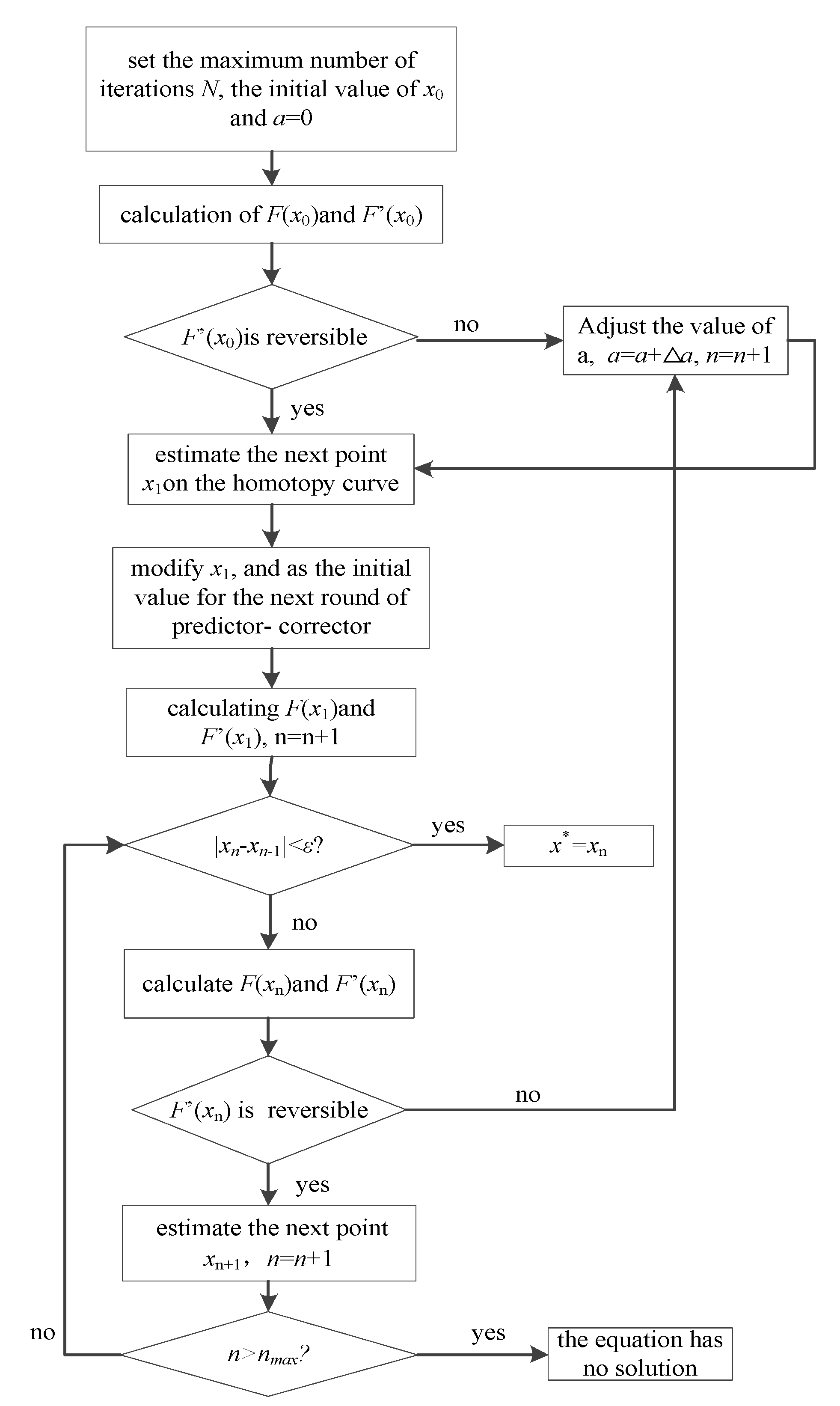
And the prediction-correction process is stopped until t = 1. After several iterations, x_n+1 may not be the exact solution x*, according to mathematical convergence theory. If |x_n+1 − x_n| < ε (ε is the set of coefficients of accuracy), it is considered that the exact solution is found, otherwise the above steps are repeated to perform the predictive-correction process. In order to elucidate the adaptive homotopy algorithm further, Figure 2 shows a flow diagram of this algorithm, which was implemented in MATLAB.

• Step 1: Set the maximum number of iterations n_max, the initial value x₀ and a = 0;
• Step 2: According to Equation (9), calculate F(x₀) and F′(x₀);
• Step 3: Judge the reversibility of F′(x₀), if YES, then turn to step 4, if not, then turn to step 9;
• Step 4: Based on Equation (18), estimate the next point x₁;
• Step 5: According to Equation (20), modify x₁ and choose the modified x₁ as the initial value for the next round. Meanwhile calculate F(x₁) and F′(x₁), n set as n + 1;
• Step 6: Assume that nth step has been carried out and obtain the solution x_n. judge whether the inequality |x_n − x_n−1| < ε is true or not. If YES, output the exact solution x* = x_n, otherwise turn step 7;
• Step 7: Calculate F(x_n) and F′(x_n), and judge whether F′(x_n) is reversible or not. If YES, based on Equation (18), estimate the next point x_n+1, and n automatically add 1, namely, n = n + 1. If not, turn step 9;
• Step 8: Judge whether the inequality n > n_max is true or not. If YES, the equation without solution. If not, then turn step 6;
• Step 9: Adjust the value of a, and define a = a + Δa. n automatically add 1, namely, n = n + 1, and turn to step 3.

4. Parameter Estimation

4.1. Weibull Distribution Parameters Estimation

There are two reasons which may lead to the relay protection equipment withdrawal from the power system. One is its failure, and the other one is the maintenance. The former possesses fault data and belongs to the corrective maintenance (CM). The latter possesses the truncated data and belongs to the preventive maintenance (PM). If the relay protection equipment is still running at the end of the observation, the data can also be censored. Considering the censored data, based on maximum likelihood, the parameters’ estimation can be described as follows:

The failure time at 0 < t_i < … < t_n (T) is observed in the time interval (0 T]. MLE is used to calculate the parameters of GPHM. It is supposed that (t_i, z_i, δ_i) and (i = 1, 2, …, n) are the records of failure and maintenance, respectively; n is the total number of events, including all the CM times and all the PM times, so that n can be expressed as n = N_cm(t) + N_pm(t). t_i is the failure time of PM and CM; z_i is the state information of the equipment at t_i, δ_i is corresponding censoring indicator variables, and the equation δ_i = 0 represents no failure at t_i. The equation δ_i = 1 represents failure at t_i.

The corresponding likelihood function is given as:

$$L(\beta ,\eta )={\displaystyle \prod _{i=1}^{l}f(t_i}{)}^{{}^{{\delta }_i}}R{(t_i)}^{{}^{1-{\delta }_i}}$$

(21)

Defining f(t) = R(t)λ(t), then

$$R(t)=\exp [-{\displaystyle {\int }_0^t{\lambda }_0(t)\exp (\gamma Z(t)})]$$

(22)

Therefore, Equation (21) can be converted into

$$\begin{array}{ll}L(\beta ,\eta )& ={\displaystyle \prod _{i=1}^{l}f(t_i}{)}^{{\delta }_i}R{(t_i)}^{1-{\delta }_i}\\ & ={\displaystyle \prod _{i=1}^r\lambda (t_i}){\displaystyle \prod _{i=1}^{l}R(t_i)}\\ & ={\displaystyle \prod _{i=1}^r\frac{\beta }{\eta }{(\frac{t_i}{\eta })}^{\beta -1}}\exp ({\displaystyle \sum _{j=1}^6{\gamma }_j{Z}_j(t_i)})\ast \\ & \hspace{1em}{\displaystyle \prod _{i=1}^l\exp (-{\displaystyle {\int }_0^T\frac{\beta }{\eta }{(\frac{t_i}{\eta })}^{\beta -1}})\exp ({\displaystyle \sum _{j=1}^6{\gamma }_j{Z}_j(t_i)}))}\end{array}$$

(23)

Here, l represents the total number of the relay protection equipment and r represents the number of faulty relay protection equipment. Then, the corresponding log likelihood function is:

$$\begin{array}{ll}\ln L=& r\ln \frac{\beta }{\eta }+{\displaystyle \sum _{i=1}^r[(\beta -1})\ln (\frac{t_i}{\eta })+{\displaystyle \sum _{j=1}^6{\gamma }_j{Z}_j(t_i)}]\\ & -{\displaystyle \sum _{i=1}^n({(\frac{t_i}{\eta })}^{\beta }.\exp {\displaystyle \sum _{j=1}^6{\gamma }_j{Z}_j(t_i)}})\end{array}$$

(24)

Taking the partial derivatives of β and η separately:

$$\frac{\partial \ln L}{\partial \beta }=\frac{r}{\beta }{\displaystyle \sum _{i=1}^r\ln }(\frac{t_i}{\eta })-{\displaystyle \sum _{i=1}^n{(\frac{t_i}{\eta })}^{\beta }.\ln (\frac{t_i}{\eta })}.\exp ({\displaystyle \sum _{j=1}^6{\gamma }_j{Z}_j(t_i)})$$

(25)

$$\frac{\partial \ln L}{\partial \eta }=-\frac{\beta r}{\eta }+{\displaystyle \sum _{i=1}^n}+\frac{\beta }{\eta }{(\frac{t_i}{\eta })}^{\beta }\exp {\displaystyle \sum _{j=1}^6{\gamma }_j{Z}_j(t_i)}$$

(26)

The maximum likelihood functions are:

$$\frac{\partial \ln L}{\partial \beta }=0$$

(27)

$$\frac{\partial \ln L}{\partial \eta }=0$$

(28)

Taking the second derivative operations, then:

$$\frac{{\partial }^2\ln L}{\partial {\beta }^2}=-\frac{r}{{\beta }^2}-{\displaystyle \sum _{i=1}^n{(\frac{t_i}{\eta })}^{\beta }[\ln }(\frac{t_i}{\eta }){]}^2\exp ({\displaystyle \sum _{j=1}^6{\gamma }_j{Z}_j(t_i)})$$

(29)

$$\frac{{\partial }^2\ln L}{\partial {\eta }^2}=-\frac{r\beta }{{\eta }^2}-{\displaystyle \sum _{i=1}^n}{(\frac{t_i}{\eta })}^{\beta }.\frac{{\beta }^2+\beta }{{\eta }^2}\exp ({\displaystyle \sum _{j=1}^6{\gamma }_j{Z}_j(t_i)})$$

(30)

$$\frac{{\partial }^2\ln L}{\partial \beta \partial \eta }=-\frac{r}{\eta }+{\displaystyle \sum _{i=1}^n\frac{1}{\eta }{(\frac{t_i}{\eta })}^{\beta }[1+\beta \ln }{t}_i]\exp ({\displaystyle \sum _{j=1}^6{\gamma }_j{Z}_j(t_i)})$$

(31)

$$\frac{{\partial }^2\ln L}{\partial \eta \partial \beta }=-\frac{r}{\eta }+{\displaystyle \sum _{i=1}^n\frac{1}{\eta }{(\frac{t_i}{\eta })}^{\beta }[1+\beta \ln }{t}_i]\exp ({\displaystyle \sum _{j=1}^6{\gamma }_j{Z}_j(t_i)})$$

(32)

Then, a second order derivative matrix can be obtained, namely Jacobi matrix:

$$J=\left[\begin{array}{cc}\frac{{\partial }^2\ln L}{\partial {\beta }^2}& \frac{{\partial }^2\ln L}{\partial \beta \partial \eta }\\ \frac{{\partial }^2\ln L}{\partial \eta \partial \beta }& \frac{{\partial }^2\ln L}{\partial {\eta }^2}\end{array}\right]$$

(33)

4.2. The Solution of Nonlinear Equations Based on Adaptive Homotopy Algorithm

According to the adaptive homotopy algorithm mentioned, the iteration equation is:

$${\left(\begin{array}{l}\beta \\ \eta \end{array}\right)}_{k+1}={\left(\begin{array}{l}\beta \\ \eta \end{array}\right)}_k-{(J_k+a_k(1-t^2)I)}^{-1}\left(\begin{array}{l}\frac{\partial \ln L}{\partial \beta }\\ \frac{\partial \ln L}{\partial \eta }\end{array}\right)$$

(34)

Here, β₀ and η₀ are the initial values of corresponding parameters when k = 0. After the initial values are selected, two parameters can be calculated according to the Equation (34).

4.3. Calculation of the Initial Value

Selecting two data points, namely, (t_d, λ_d) and (t_g, λ_g) in the Weibull distribution, the initial values can be solved by the following equation.

$$\{\begin{array}{c}\frac{{\beta }_0}{{\eta }_0}{(\frac{t_d}{{\eta }_0})}^{\beta -1}={\lambda }_d\\ \frac{{\beta }_0}{{\eta }_0}{(\frac{t_g}{{\eta }_0})}^{\beta -1}={\lambda }_g\end{array}$$

(35)

According to the above analysis, MLE can be used to estimate the parameter of GPHM. And the adaptive homotopy algorithm can be used to solve the nonlinear equation in the parameter estimation process. Then, the fault rate model is established.

5. Case Analysis

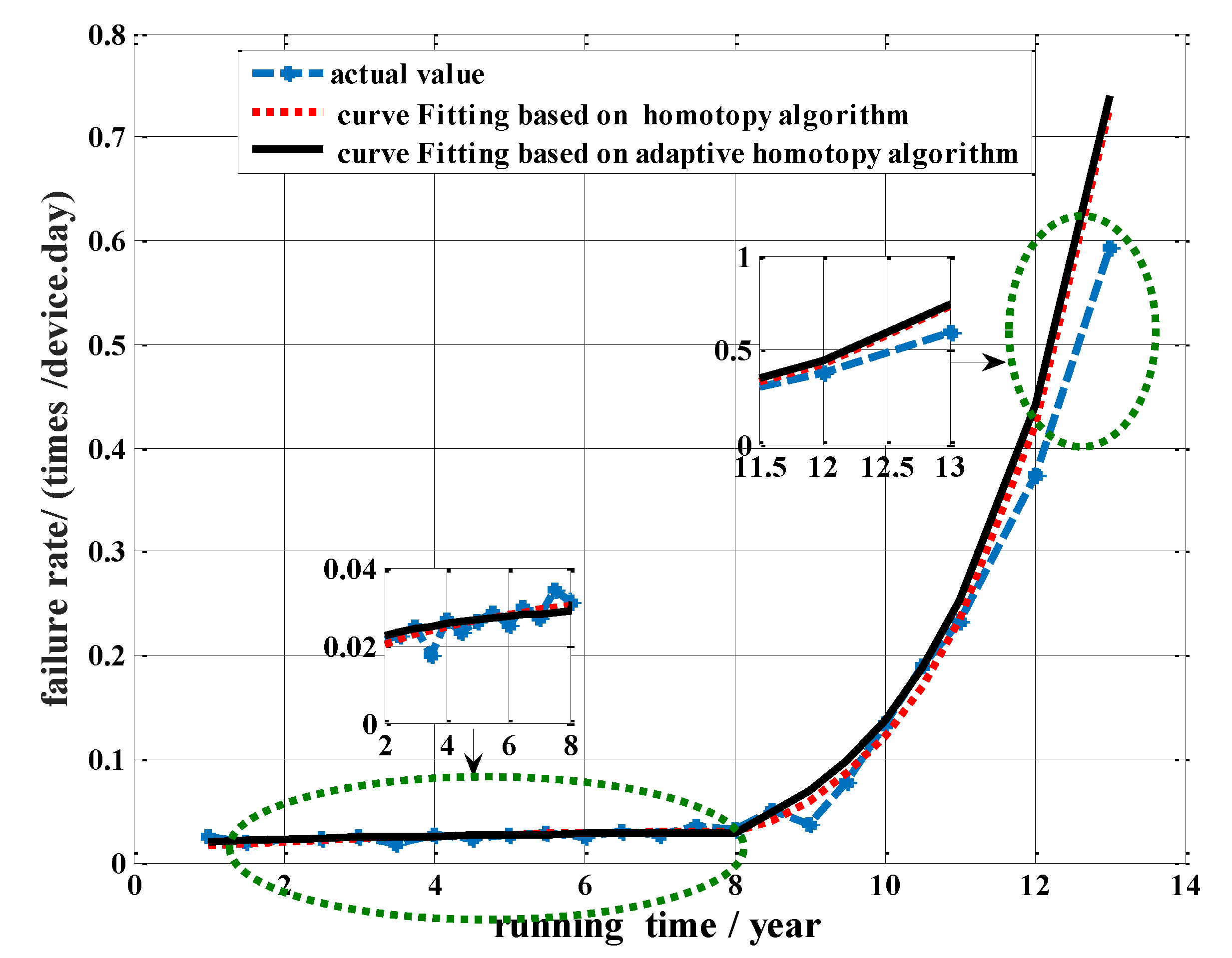
Case 1: The machine account and defect information of the relay protection equipment are collected, which are running in the similar environment or have the same type, and its failure rate is shown in

Table 4. Statistics of failure rate of relay protection.

Running Time/Year	Failure Rate/(Times/Device. Year)	Running Time/Year	Failure Rate (Times/Device. Year)
1	0.0251	7	0.0272
1.5	0.0202	7.5	0.0342
2.5	0.0226	8	0.0311
3	0.025	8.5	0.0496
3.5	0.0177	9	0.0364
4	0.0268	9.5	0.0774
4.5	0.0232	10	0.133
5	0.0261	10.5	0.189
5.5	0.0283	11	0.232
6	0.0253	12	0.374
6.5	0.0296	13	0.593

. According the above failure rate, the failure rate curve can be drawn as Figure 3 shown. Based on the adaptive homotopy algorithm and the Newton homotopy algorithm, the failure rate parameters are computed iteratively. Then, failure rate parameters of the Weibull distribution can be obtained and shown in

Table 5. Estimation of parameters based on adaptive homotopy algorithm.

Stage of Fault Distribution	Random Failure Period		Loss Failure Period
	β	η	β	η
parameter values	1.2903	29.1759	7.818	12.526
relative error	0.0971		0.1711
iteration number	5

and

Table 6. Estimation of parameters based on Newton homotopy algorithm.

Stage of Fault Distribution	Random Failure Period		Loss Failure Period
	β	η	β	η
parameter values	1.177	31.936	7.248	12.435
relative error	0.1532		0.2518
iteration number	11

, so that their fitting curve can also be seen in Figure 3.

Through analyzing the data of Table 5 and Table 6 and the curves in Figure 3, the iterations number of the adaptive homotopy algorithm is significantly smaller the iterations number of other algorithms. When the equipment is in the random failure period, the relative error of the adaptive homotopy algorithm is 0.0971, and the Newton homotopy algorithm is 0.1532. When the equipment is in the loss failure period, the relative error of the adaptive homotopy method is 0.1711 and the Newton homotopy algorithm is 0.2518, whose error is large. This is caused by the fact that when the equipment is running, all parts of the equipment occur material fatigue, aging or rust and other undesirable conditions. In order to ensure the normal operation of the equipment, the appropriate maintenance should be done, namely, PM, or CM. However, these two types of maintenance inevitably affect the equipment failure rate. Therefore, the model considering the run-time regardless of the current state will be not correct. The result has big difference with the actual operation.

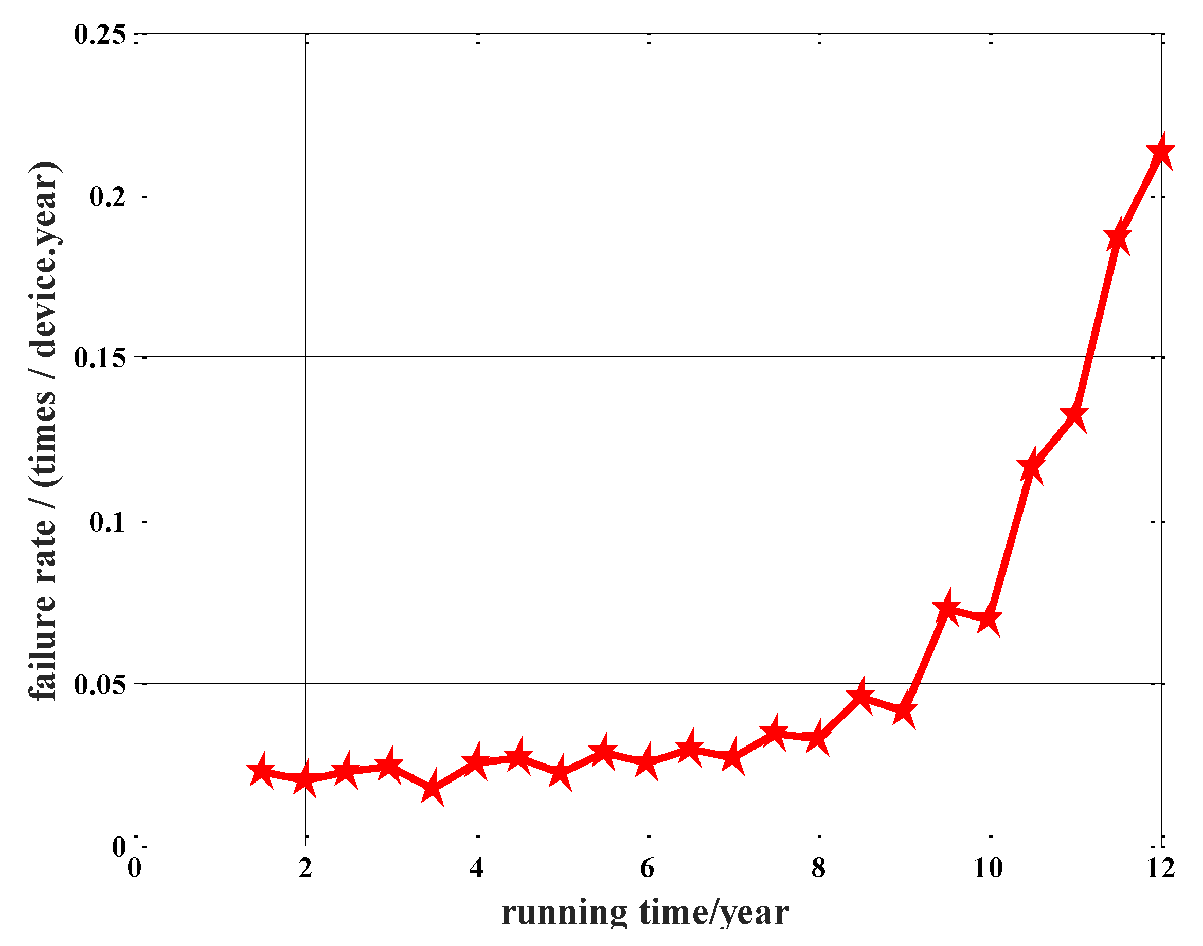
Case 2: Similar to case 1, the operation data of relay protection equipment is shown in

Table 7. Operation data of relay protection.

Running Time/Year	Failure Rate (Times/Device. Year)	Running Time/Year	Failure Rate (Times/Device. Year)
1.5	0.0224	7.0	0.0268
2	0.0202	7.5	0.0342
2.5	0.0226	8.0	0.0327
3	0.024	8.5	0.0453
3.5	0.0175	9.0	0.0411
4	0.0252	9.5	0.0726
4.5	0.0267	10.0	0.0693
5	0.0223	10.5	0.116
5.5	0.0283	11	0.132
6	0.0253	11.5	0.187
6.5	0.0296	12	0.213

. Based on Table 7, the failure rate curve of relay protection equipment can be obtained in Figure 4.

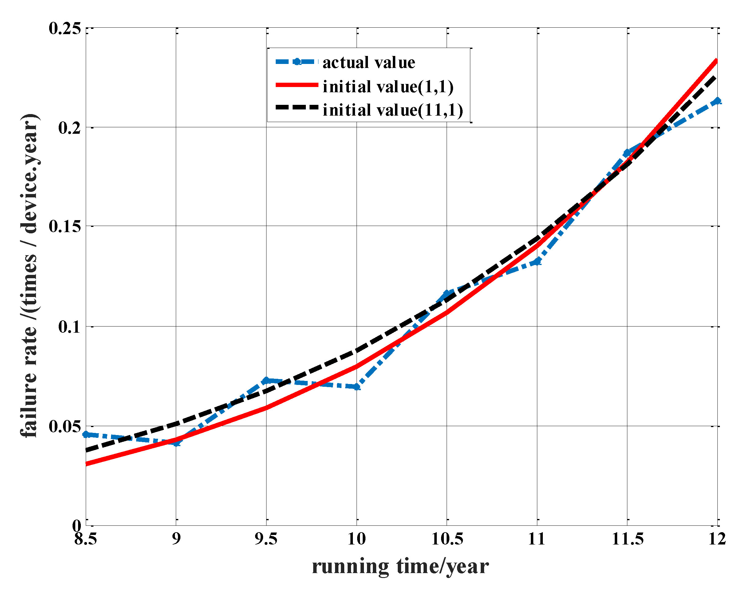
Based on the data from Table 7, the convergence characteristics of different algorithms can be obtained. From

Table 8. Comparisons of two algorithms.

Initial Value	Newton Homotopy Algorithm		Adaptive Homotopy Algorithm
	convergence	(β, η)	convergence	iteration number	a	(β, η)
(1, 1)	non-converging	-	convergence	10	3	6.201, 13.790
(11, 1)	non-converging	-	convergence	35	−1	6.201, 12.971

, it can be found that the Newton homotopy algorithm is non-converging. However, the adaptive homotopy algorithm can guarantee the singularity of the equation by controlling the parameter a. According to Equation (15), a_n affects singularity of nonlinear equations, so that the optimal parameter a is selected which can make the iteration number need less. According to Table 8, although there will be differences between the initial values/parameter values/iterations number, the difference of the final parameter estimates’ results are in the allowed error range. Therefore, it can be proved that the homotopy algorithm is independent of the setting of the initial value, and the different initial values are the different optimal values of a. For example, when the initial value is (1, 1), the iteration number is 10, and then the optimal value of a is 3. While the initial value is (11, 1), the iteration number is 35, and then the optimal value of a is −1. Figure 5 shows the curves corresponding to different initial values. From Figure 5, the trend of the curve can fully verify the above analysis results.

Case 3: It is necessary to do the corresponding maintenance for equipment after the device is put into operation for some time. According to Equation (15), it can be found that the choice of maintenance can affect the failure rate.

Table 9. Operation data of relay protection equipment.

Running Time/Day	Failure Rate/(Times/Device. Day)	Running Time/Day	Failure Rate/(Times/Device. Day)
215	0.0130	1300	0.0186
310	0.0141	1557	0.0212
471	0.0182	1754	0.0215
680	0.024	1891	0.0200
763	0.0221	2058	0.0211
841	0.0202	2177	0.0200
1008	0.0168	2482	0.066168
1193	0.019

gives the operating data of the equipment maintenance. In order to solve the parameters of GPHM, the life data of relay protection equipment is analyzed, firstly. Then, the regression coefficient vector γ is estimated by Statistical Analysis Software (SPSS). On the basis of γ, the adaptive homotopy algorithm is used to estimate the other parameters.

Model I: selecting the times of maintenance as a covariate; Models II/III: on the basis of model I, the condition monitoring data of the corrective or preventive maintenance moment are fitted, such as age, the operating environment, the HI of equipment, and the manufacturer; Model IV: on the basis of Models II/III, the condition monitoring data of the whole period (such as age, the operating environment, the HI of equipment, and the manufacturer) are fitted, not just the state of corrective or preventive maintenance moment.

From

Table 10. Parameter estimation of models with different factor combinations.

Model	Estimated Log Likelihood	Parameter Estimation
		β	η	γpm	γcm	γage	γenv	γHI	γmau
I	−55.409	1.424	29.58	0.013	−0.001	0	0	0	0
II	−57.940	1.25	33.49	0	−0.001	−0.001	0.911	−0.079	−0.288
III	−54.404	1.434	25.673	0.0137	0	0.0004	0.728	0.053	0.482
IV	−53.930	1.424	29.581	0.0138	−0.001	0.0003	0.773	−0.047	0.516

, by comparing the estimated log likelihood, the fourth methods are optimal and its log likelihood is −53.930. Obviously, based on the monitoring data of the entire running time, GPHM has better fitting characteristics. According to parameter estimation results, it can be found that the failure maintenances frequency, γ_cm, is negative in the above three approaches, so that CM can effectively reduce the failure rate. The preventive maintenances frequency, γ_pm, is positive, so that PM can’t effectively reduce the failure rate. This conclusion can provide a theoretical basis for maintenance personnel to choose the appropriate maintenance mode, and improve maintenance efficiency in case of the blind maintenance. The results also show that when the environment and the internal state of the covariates deviate from the rated or normal state, the failure rate will be higher. The quantitative analysis is consistent with the experience. Based on GPHM model, the curve of equipment failure rate can be obtained as Figure 5 shown. From Figure 6, we can find that the curve based on GPHM is closed to the actual value, while the Weibull model is away from the actual value, especially in the loss period. That is because in the loss period the equipment has to implement the maintenance. It is inevitable to affect the fault rate.

6. Conclusions

In order to fully analyze the impact of the whole process of the monitoring state on the failure rate, this paper presents GPHM-Weibull, whose covariates include the times of PM and CM, age, the operating environment, HI, and manufacturer. The baseline function obeys Weibull distribution, and the adaptive homotopy algorithm is adopted to estimate the parameters of Weibull distribution. The regression coefficient vector γ is estimated by SPSS. Finally, three cases have been presented to demonstrate the following conclusions.

(1) The curve drawn by the GPHM is very close to the actual value. However, due to GPHM taking the whole running state of the equipment into consideration, the curve drawn by the Weibull model is away from the actual value, especially in the loss period.

(2) The adaptive homotopy algorithm ensures the singularity of the equation by adjusting the parameter a, and the result of the parameter estimation is less affected by the initial value.

References

1. Lin, X.; Yu, K.; Tong, N.; Li, Z.; Khalid, M.S.; Huang, J.; Li, Z.; Zhang, R. Countermeasures on preventing backup protection mal-operation during load flow transferring. Int. J. Electr. Power Energy Syst. 2016, 79, 27–33. [Google Scholar] [CrossRef]
2. Alam, M.N.; Das, B.; Pant, V. An interior point method based protection coordination scheme for directional overcurrent relays in meshed networks. Int. J. Electr. Power Energy Syst. 2016, 81, 153–164. [Google Scholar] [CrossRef]
3. Dai, Z.H.; Wang, Z.P. Overview of research on protection reliability. Power Syst. Prot. Control 2010, 38, 161–167. [Google Scholar]
4. Zhou, X. New Technology of Power System Reliability; China Electric Power Press: Beijing, China, 2014. [Google Scholar]
5. Moeini, A.; Jenab, K.; Mohammadi, M.; Foumani, M. Fitting the three-parameter Weibull distribution with Cross Entropy. Appl. Math. Model. 2013, 37, 6354–6363. [Google Scholar] [CrossRef]
6. Dombi, J.; Jónás, T.; Tóth, Z.E. Clustering Empirical Failure Rate Curves for Reliability Prediction Purposes in the Case of Consumer Electronic Products. Qual. Reliab. Eng. Int. 2015, 32, 1071–1083. [Google Scholar] [CrossRef]
7. Wang, H.; Yang, H.; He, B.; Wang, Y. Improvement of state failure rate model for Power transmission and transforming equipment. Autom. Electr. Power Syst. 2011, 15, 27–31. [Google Scholar]
8. Jahromi, A.; Piercy, R.; Cress, S.; Service, J.; Fan, W. An approach to power transformer asset management using health index. IEEE Electr. Insul. Mag. 2009, 2, 20–34. [Google Scholar] [CrossRef]
9. Hughes, D.; Dennis, G.; Walker, J.; Williamson, C. Condition Based Risk Management (CBRM)—Enabling Asset Condition Information to be Central to Corporate Decision Making; Engineering Asset Management; Springer: London, UK, 2006; pp. 1212–1217. [Google Scholar]
10. Earp, G. Condition based risk assessment of electricity towers using high resolution images from a helicopter Electricity Distribution. In Proceedings of the 18th International Conference and Exhibition on Electricity Distribution (CIRED 2005), Turin, Italy, 6–9 June 2005; IET (Britain): London, UK, 2005; pp. 1–5. [Google Scholar]
11. Chan, J.K.; Shaw, L. Modeling repairable systems with failure rates that depend on age and maintenance. IEEE Trans. Reliab. 1993, 42, 566–571. [Google Scholar] [CrossRef]
12. Dui, H.; Si, S.; Zuo, M.J.; Sun, S. Semi-Markov process-based integrated importance measure for multi-state systems. IEEE Trans. Reliab. 2015, 64, 754–765. [Google Scholar] [CrossRef]
13. Jardine, A.; Anderson, P.; Mann, D. Application of the Weibull proportional hazards model to aircraft and marine engine failure data. Qual. Reliab. Eng. Int. 1987, 3, 77–82. [Google Scholar] [CrossRef]
14. Sun, Y.; Ma, L.; Mathew, J.; Wang, W.; Zhang, S. Mechanical systems hazard estimation using condition monitoring. Mech. Syst. Signal Process. 2006, 20, 1189–1201. [Google Scholar] [CrossRef]
15. Kumar, D. Proportional hazards modelling of repairable systems. Qual. Reliab. Eng. Int. 1995, 11, 361–369. [Google Scholar] [CrossRef]
16. Syamsundar, A.; Naikan, V.N.A. Mathematical modelling of maintained systems using point processes. IMA J. Manag. Math. 2009, 20, 275–301. [Google Scholar] [CrossRef]
17. Lugtigheid, D. Modelling repairable system reliability with explanatory variables and repair and maintenance actions. IMA J. Manag. Math. 2004, 15, 89–93. [Google Scholar] [CrossRef]
18. Elsayed, E.; Chan, C. Estimation of thin-oxide reliability using proportional hazards models. IEEE Trans. Reliab. 2002, 39, 329–335. [Google Scholar] [CrossRef]
19. Li, L.; Ma, D.; Li, Z. Cox-Proportional Hazards Modeling in Reliability Analysis—A Study of Electromagnetic Relays Data. IEEE Trans. Compon. Packag. Manuf. Technol. 2015, 5, 1582–1589. [Google Scholar]
20. Zhang, R.; Cai, W.; Ni, L.; Lebby, G.L. Power system load forecasting using partial least square method. In Proceedings of the 40th Southeastern Symposium on System Theory (SSST), New Orleans, LA, USA, 16–18 March 2008; pp. 169–173. [Google Scholar]
21. Bouaricha, A.; Schnabel, R.B. Tensor methods for large sparse systems of nonlinear equations. Math. Program. 1998, 82, 377–400. [Google Scholar] [CrossRef]
22. Reif, K.; Weinzierl, K.; Zell, A.; Unbehauen, R. A homotopy approach for nonlinear control synthesis. IEEE Trans. Autom. Control 1998, 43, 1311–1318. [Google Scholar] [CrossRef]
23. Li, T.Y.; Zeng, Z.; Cong, L. Solving eigenvalue problems of real nonsymmetric matrices with real homotopies. SIAM J. Numer. Anal. 1992, 29, 229–248. [Google Scholar] [CrossRef]
24. Bayat, M.; Pakar, I.; Bayat, M. Approximate analytical solution of nonlinear systems using homotopy perturbation method. J. Process Mech. Eng. 2016, 230, 10–17. [Google Scholar] [CrossRef]
25. Kumar, D.; Westberg, U. Proportional hazards modeling of time-dependent covariates using linear regression: A case study: Mine power cable reliability. IEEE Trans. Reliab. 1996, 45, 386–392. [Google Scholar] [CrossRef]
26. Wang, H.; Zhao, W.; Du, Z. Economic Life Prediction of Power Transformers Based on the Lifetime Data. Power Syst. Technol. 2015, 39, 810–816. [Google Scholar]
27. Percy, D.F.; Kobbacy, K.A.H.; Ascher, H.E. Using proportional-intensities models to schedule preventive–maintenance intervals. IMA J. Math. Appl. Bus. Ind. 1998, 9, 289–302. [Google Scholar] [CrossRef]
28. Liu, X.; Shahidehpour, M.; Cao, Y.; Li, Z.; Tian, W. Risk Assessment in Extreme Events Considering the Reliability of Protection Systems. IEEE Trans. Smart Grid 2015, 6, 1073–1081. [Google Scholar] [CrossRef]
Figure 1. Selection of covariates.
Processes 07 00899 g001
Figure 2. Calculation flow chart of adaptive homotopy algorithm.
Processes 07 00899 g002
Figure 3. Curve fitting of failure rate.
Processes 07 00899 g003
Figure 4. The failure rate curve of equipment.
Processes 07 00899 g004
Figure 5. The failure rate curve of equipment.
Processes 07 00899 g005
Figure 6. Curve fitting based on the generalized proportional hazard model (GPHM).
Processes 07 00899 g006