Development of New Algorithm for Aniline Point Estimation of Petroleum Fraction

Abstract

The aniline point (AP) is an important physical property of a petroleum fraction. The AP gives an indication of the aromatic hydrocarbon content in a hydrocarbon mixture and can also be an indicator of the ignition point of a diesel fraction. In this study, common estimation methods were introduced and evaluated, and their limitations were analyzed. Multiple linear regression was used in constructing a quantitative function to solve for the AP using the average boiling point and specific gravity. The iterative modification algorithm of the ternary interaction algorithm was used to obtain the predicted value of the petroleum fraction AP, and the proposed algorithm was tested using 127 actual petroleum fractions. The average estimation deviation of the proposed method was 3.55%; hence, compared to the commonly used estimation methods, the prediction accuracy was significantly improved. This method offers important practical value in the calculation of the petroleum fraction AP and other petroleum fraction properties, thereby providing reference significance.

1. Introduction

During the petroleum (such as gasoline and diesel oil) production process, the real-time monitoring of oil products is the most direct means of ensuring production safety and maintaining oil quality stability. The aniline point (AP) [1] is defined as the lowest temperature at which an equal volume of aniline (C6H7N) is completely miscible with the tested sample. The AP temperature contributes to the characterization of pure hydrocarbons and the analysis of hydrocarbon mixtures. It is commonly used to estimate the aromatic content of petroleum, and it is therefore important for determining the composition of petroleum fractions and the quality of petroleum products. Petroleum feedstocks with high APs have higher alkane contents and lower amounts of aromatics and naphthenes. APs can also be used to calculate petroleum fraction properties, such as combustion heat, the hydrogen content, the diesel index, and the smoke point [2,3].

At present, experimental methods for determining the AP are usually developed according to the domestic general standard, GB/T 262-2010 [4]. Equal volumes of aniline and the solvent to be tested are mixed, the mixture is heated at a constant rate until the two phases become completely miscible, and then the mixture is cooled at a constant rate. The temperature at which the two phases separate is recorded as the AP. In general, a higher content of aromatics results in a lower AP, while a higher alkane content results in a higher AP. The AP of cycloalkane and olefin is somewhere between these values. When experimental values of APs are not available or cannot be determined, a convenient and rapid method for predicting the APs must be used [5]. Yonggang has suggested that the aniline purification level and the cooling rate have a significant influence on AP determination [2]. It is very difficult to determine the AP of the petroleum fraction experimentally. Huizhen combined an artificial neural network (ANN) and the group contribution method to predict petroleum fraction physical properties and substituted the predicted value of the group into the AP ANN model to improve the estimation accuracy [3]. Farhad used a genetic algorithm and multiple linear regression to statistically validate molecular descriptors in pure hydrocarbons and returned multilinear models to generate neural networks to effectively predict pure hydrocarbon APs [1,5], which were pure components. some new methods have also been provided to estimate APs, e.g., Yinyan conducted a quantitative structure–property relationship (QSPR) study on the APs of 126 hydrocarbons from a molecular structure perspective and realized a function predicting the APs of hydrocarbons based on their molecular structure [6]. Although the above methods are advanced, they are not suitable for engineering computing applications, and their accuracy has not been systematically verified. On the basis of the difference in the properties of the estimated materials, the aniline point estimation method can be divided into a pure component aniline point estimation method and a petroleum fraction aniline point estimation method. At present, methods for estimating models, such as the genetic algorithm-multiple linear regression (GA-MLR), have been established, and structural parameters reflecting molecular structure information are calculated based on molecular structure. This method uses a genetic function algorithm to select the structural parameters that are closely related to the aniline point of hydrocarbons from many structural parameters. The algorithm then uses these parameters as a molecular description to characterize the structural characteristics of the corresponding compounds. Thereafter, multiple linear regression is used to establish predictive hydrocarbons. Using this model, the target properties can be quickly calculated and predicted, and the kinetic energy of the aniline point of hydrocarbons can be predicted according to the molecular structure. This is of great significance in the estimation of aniline points of petroleum fractions.

In the estimation process of the petroleum fraction model, there are enormous challenges to accurately estimating its characteristics [7,8,9] due to the diverse components in the material. Therefore, on the basis of the analysis and fitting of petroleum fraction physical properties, it is good to establish an aniline point estimation model for petroleum fractions. Actual estimation methods that are commonly used in domestic and foreign research include the American Petroleum Institute (API) method [10], Winn method [11], Linden method [12], Walsh–Mortimer method [13], and Albahari method [14]. The estimation of APs has also been researched extensively by local scholars, including Chen Xionghua [15] and Shoude Qing [16]. However, these algorithms have certain defects in terms of practical applications: the accuracy of the Winn method depends on the accuracy of the input parameters; the limitation of the Linden method is that the correlation was originally developed based on only 37 original datapoints, and hence the estimation of other petroleum fractions may induce a large deviation; the difficulty of the Walsh–Mortimer method is that it is necessary to accurately find a normal paraffin with the same normal boiling point and average boiling point; a model extrapolation of the Shoudeqing method cannot be applied to a wide range of petroleum fractions, and the verification experiment is performed afterward; and the Albahri method uses the refractive index as a basic characteristic variable (the effect is unknown, which will be further verified below). Evaluation results of the above seven commonly used model evaluations have demonstrated that the API and Chen–Xionghua methods exhibit the lowest deviation from the AP estimation, and an analysis of the correlation formula has indicated that the average boiling point and specific gravity (the API gravity is calculated by the specific gravity) have a significant effect on the AP. The AP is not just linearly associated with the average boiling point or specific gravity, but it is also related to the interaction between the two parameters [17]. The aniline point estimation methods that have been established by the group contribution method, artificial neural networks, and genetic algorithms have mostly been used for the estimation of pure hydrocarbon aniline points. Due to the special nature of the petroleum fraction, the aniline point should be estimated using an empirically relevant method.

This study introduces seven methods that are commonly used in the estimation of APs in petroleum fractions. An analysis and evaluation of these methods is presented. A new algorithm is proposed to improve the accuracy of AP estimation.

2. Common AP Estimation Methods and Evaluation

2.1. Common AP Estimation Models

2.1.1. API Method

The API Technical Data Book uses the mean average boiling point, specific gravity, and Watson characteristic factor of the petroleum fraction to predict the petroleum fraction AP, according to the following model [10]:

$$AP=-969.65-0.139MeABP+59.889K_w+482.611SG,$$

(1)

$$K_w=\frac{1.8MeAB{P}^{1/3}}{SG}.$$

(2)

2.1.2. Winn Method

In the Winn method, the AP is obtained from the correlation between the mean average boiling point and the API gravity or specific gravity [11]. According to the Winn nomogram, the aniline point can also be obtained from the correlation between the mean average boiling point and the API gravity or specific gravity as follows: take the point mapping, use the quasi-Newton method (BFGS) and the general global optimization method for fitting, and get the correlation of R = 1, as shown in Figure 1

Equation (3) is

$$\begin{array}{c}AP=316.66-\frac{1223.20}{1+{\left(\left(MeABP-28.62\right)/175.55\right)}^2}-\frac{32.65}{1+\left(1+{\left(\left(31.40-API\right)/3.20\right)}^2\right)}\\ -\frac{2.59}{\left(1+{\left(\left(MeABP-28.62\right)/175.55\right)}^2\right)\left(1+{\left(\left(31.40-API\right)/3.20\right)}^2\right)}\end{array}$$

(3)

2.1.3. Linden Method

According to the characterization methods of Watson and Nelson, the approach proposed by Linden uses the API gravity and mean average boiling point to predict the AP of the petroleum fraction [12], as follows:

$$AP=-183.3+0.27API·MeAB{P}^{1/3}+0.317MeABP,$$

(4)

$$API=\frac{141.5}{SG}-131.5.$$

(5)

2.1.4. Walsh–Mortimer Method

On the basis of the study of gas chromatography, Walsh and Mortimer proposed that the AP is predicted by a polynomial of the carbon content and the specific gravity of normal paraffin, with the normal boiling point equal to the mean average boiling point [13,18]:

$$AP=-204.9-1.498C_{50}+\frac{100.5C_{50}^{1/3}}{SG},$$

(6)

$$C_{50}=\frac{M_P-14}{2},$$

(7)

$$M_P={\left[\frac{6.98291-\ln \left(1070-MeABP\right)}{0.02013}\right]}^{3/2}.$$

(8)

2.1.5. Albahri Method

This method uses the refractive index as a basic characteristic parameter to predict the AP of the petroleum fraction [14,19]:

$$AP=-9805.269R_i+711.85761SG+9778.7069,$$

(9)

$$R_i=n_{20}-\frac{d_{20}}{2},$$

(10)

$$n_{20}={\left(\frac{1+2I}{1-2I}\right)}^{\frac{1}{2}},$$

(11)

$$I=0.012419MeAB{P}^{0.006438}S{G}^{-1.6117}{e}^{0.0007272MeABP+3.3223SG-0.0008867MeABP·SG},$$

(12)

$$d_{20}=SG-0.0045\left(2.34-1.9SG\right).$$

(13)

2.1.6. Chen–Xionghua (Chen)

In this method, the API gravity and the mean average boiling point of 65 petroleum fractions are used as the parameters, and the measured AP value is employed as the standard to fit the correlation formula [15]:

$$AP=-140.9942+3.6913API+0.4618MeABP-0.0224AP{I}^2-0.00025305MeAB{P}^2.$$

(14)

2.1.7. Shoude Qing (Shou)

By measuring 174 petroleum fractions of six representative crude oils, including Daqing, Shengli, Dagang, Renqiu, Gudao, and Yangsanmu, as well as the catalytic cracking distillates of Daqing and Shengli (reforming and extracting oil) and the winning coking fractions, the physical properties (e.g., the mean average boiling point, density, and AP) of 95 petroleum fractions of representative secondary processing oils are determined. Using the above data as parameters, the empirical correlation of the estimated AP is obtained through Equation (15) [7,16]:

$$AP=1.63677\times {10}^{-5}MeAB{P}^{2.29383}S{G}^{-4.40113}.$$

(15)

2.2. Data Sources

From the actual oil products provided by the factory, 24 petroleum fractions within the applicable range were selected for testing and compared to the measured values. These 24 petroleum fractions were from the literature [3]. The average relative deviation (ARD) and average absolute deviation (AAD) of the predicted results were calculated. The oil APs used for verification ranged from 45 to 107 °C, the average boiling point ranged from 115 to 545 °C, and the API gravity ranged from 14 to 56.

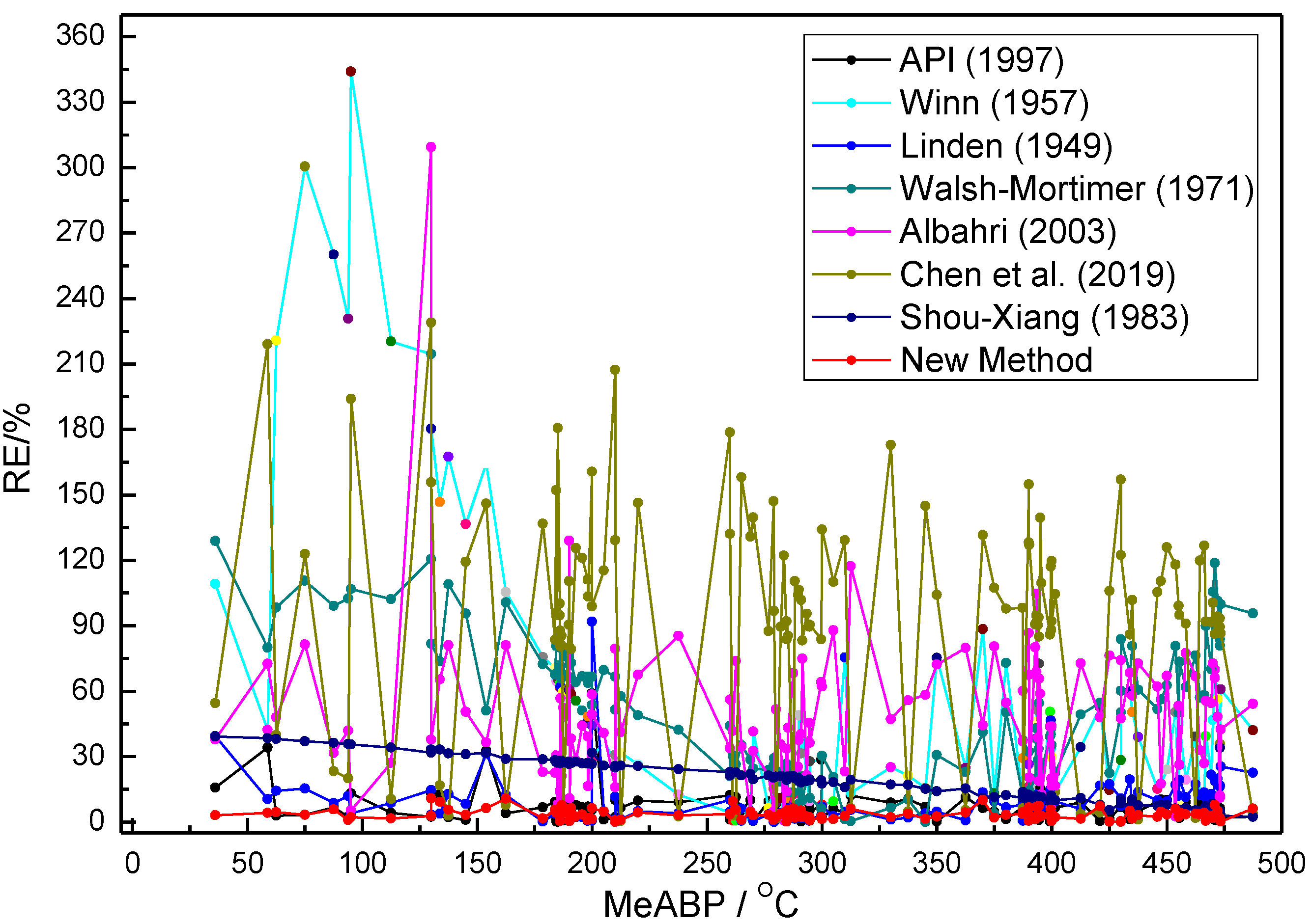
2.3. Evaluation Results

A comparison of the evaluation results of the seven algorithms introduced above is presented in

Table 1. Error analysis of existing aniline point (AP) estimation methods. ARD: average relative deviation; AAD: average absolute deviation.

Method	ARD (%)	AAD (°C)
API Method	7.31	5.44
Winn Method	28.32	10.65
Walsh–Mortimer Method	9.46	6.74
Linden Method	12.28	12.93
Albahri Method	10.66	15.07
Chen Method	9.83	6.46
Shou Method	22.54	19.11

.

As can be observed from Table 1, the AADs of the seven estimation methods were 5.44 °C, 10.65 °C, 6.74 °C, 12.93 °C, 15.07 °C, 6.46 °C, and 19.11 °C. The ARDs of the seven methods were approximately 7.31% to 28.32%, and the minimum ARD was above 5%. The error in the method was obtained as follows: the accuracy of the Winn method depends on the accuracy of the input parameters. The limitation of the Linden method is that the correlation was originally developed based on only 37 original datapoints. Thus, the estimated ARD for other petroleum fractions was 12.28%. The difficulty of the Walsh–Mortimer method is that it is necessary to accurately determine normal paraffin with the same normal boiling point and medium average boiling point. The estimated ARD and ADD of the Shou method were the biggest among the evaluated methods, which showed that the model extrapolation was not strong. The ARD of the Albahri method was 10.66%. The ARDs of the API and the Chen–Xionghua methods were 7.31% and 9.83%, which were both less than 10%, indicating that using the refractive index as a basic characteristic variable is not as effective in the API method and that the model prediction effect of the Chen–Xionghua method is accurate. Although the API method showed a minimum deviation of 7.31% when estimating 24 kinds of real oil, this was still more than 5%, which makes it difficult to meet the high accuracy of the actual estimation.

In summary, the commonly used AP estimation models had a medium average boiling point range of 115 to 545 °C and an API gravity range of 14 to 56. In actual oil products, the calculation results exhibited significant deviations, which is difficult to handle in practice. Therefore, estimation is necessary, and a more accurate AP estimation model is required. With reference to the variables used in the API method, it is suggested that a new average model and the actual values of real oil be used to return a new average correlation.

3. New Algorithm for AP Estimation

3.1. Proposal of New Model for AP

To avoid the singularity of the previous methods, the complex interactions between the three should be considered. Thus, the formula for estimating the petroleum fraction AP is as follows:

$$AP=f(MeABP)+g(SG)+h(MeABP,SG).$$

(16)

As is indicated in Equation (16), the model consists of three parts: f(MeABP), which is affected by the mean average boiling point; g(SG), which is affected by the specific gravity; and h(MeABP, SG), which is affected by the interaction between the mean average boiling point and specific gravity.

For the univariate regression terms f(MeABP) and g(SG), a total of 142 actual oil data points were used, which were derived from the existing literature and measured values [8,9,20]. These 142 data points can be recorded in detail in Appendix A,

Table A1. Summary of 142 oil datapoints measured for regression models.

No.	Specific Gravity (15.5 °C)	Average Boiling Point (K)	Aniline Point Experimental Value (K)	New Method (K)
1	0.5164	306.95	326.92	326.22
2	0.5191	373.15	359.01	355.70
3	0.5449	371.09	358.32	358.01
4	0.5606	371.09	358.32	359.05
5	0.5606	333.35	342.78	343.70
6	0.5612	371.09	358.32	359.01
7	0.6275	674.62	406.79	408.01
8	0.6562	373.15	356.79	356.70
9	0.6623	763.66	412.43	413.89
10	0.6673	208.50	307.79	307.48
11	0.6928	360.86	335.18	335.88
12	0.7163	292.36	264.93	265.50
13	0.7163	371.09	327.72	327.07
14	0.7423	542.68	374.48	378.93
16	0.7596	542.68	370.08	369.93
17	0.7596	417.80	329.40	328.68
18	0.7606	673.21	390.90	389.38
19	0.7606	211.59	236.06	235.82
20	0.7606	278.20	236.06	235.52
21	0.7606	301.10	236.90	309.05
22	0.7606	338.59	266.02	266.12
23	0.7606	338.59	338.59	337.18
24	0.7658	257.19	233.21	233.30
25	0.8425	430.51	280.68	280.77
26	0.8500	333.35	209.79	209.56
27	0.8316	542.68	346.99	351.93
28	0.8114	542.68	354.40	355.93
29	0.8066	542.68	356.04	357.13
30	0.8110	542.41	354.46	353.21
31	0.8118	536.28	352.42	354.21
32	0.8010	508.35	347.82	346.84
33	0.8222	508.35	338.98	337.84
34	0.8440	367.67	232.41	232.51
35	0.8460	367.67	231.25	230.51
36	0.7930	371.09	269.51	268.29
37	0.8370	371.09	238.86	239.29
38	0.8232	672.28	378.54	378.09
39	0.8217	360.86	199.07	198.42
40	0.8001	317.87	317.87	316.45
41	0.8477	752.27	385.48	388.18
42	0.7772	257.16	227.24	227.82
43	0.8104	194.58	211.34	211.82
44	0.7658	257.16	172.40	172.82
Boscan	1.0354	746.00	328.42	327.28
Buzurgan	1.0285	661.00	297.48	295.56
Cambimas vacuum	1.0298	622.00	274.46	274.82
D.A. feed crack stock	1.0246	687.00	311.70	310.31
D.A. feed lube oil	1.0231	693.00	314.96	314.85
D-1 diesel oil (avg)	0.9541	578.00	299.99	299.45
DAO C4	1.0100	781.00	348.12	347.71
DAO L.O	1.0246	804.00	348.45	349.11
Diesel oil T-097-96	0.9529	578.00	300.75	300.42
F.C.C. heavy gas oil M.C.	1.0000	688.00	324.35	324.94
Gasoline 31 API #1	0.9321	572.00	310.29	310.68
Hydroc. Feed VGO	1.0025	697.00	326.44	327.22
Kerosene 31 API #2	0.9242	574.00	315.78	315.79
Kuwait crude cut #7	0.8753	613.00	351.52	353.09
Kuwait vacuum	1.0254	682.00	309.12	308.80
Petroleum cut #2	0.9590	578.00	296.84	296.15
Petroleum cut #3	0.9710	447.00	202.84	202.22
Vacuum gas oil 31 API #2	0.9485	713.00	352.44	353.87
Vacuum gas oil crude assay 91	0.9107	676.00	355.81	354.47
Arabian light atmosphere	1.0328	740.00	327.59	325.75
Athambasaca	1.0366	697.00	309.57	311.28
Atmospheric residue crude assay 84	0.9189	752.00	369.49	370.60
Atmospheric residue crude assay 91	0.9189	752.00	369.49	369.62
Atmospheric residue crude assay 94	0.9107	748.00	370.86	371.99
Cold Lake	1.0513	722.00	312.24	313.25
DAO C5	1.0209	772.00	341.91	342.37
Deasphalting unit DAO C4	0.9800	548.00	262.43	262.36
Deasphalting unit DAO C5	0.9923	772.00	352.01	352.48
Deasphalting unit DAO(lube oil)	1.0000	804.00	356.52	355.45
Deasphalting unit feed	0.9760	525.00	249.21	249.11
Deasphalting unit feed	1.0030	739.00	339.64	338.55
Deasphalting unit feed lube oil	0.9979	693.00	327.13	327.85
Diesel oil T-106-96	0.9491	578.00	303.13	302.45
FCC H. G.O cut M.C.	1.0030	688.00	322.93	325.08
Gasoline 31 API #2	0.9367	583.00	313.03	313.20
Hydroc. VGO	1.0000	683.00	322.49	322.65
Jobo	1.0768	728.00	301.12	300.98
Kerosene 31 API #1	0.9240	585.00	320.87	320.79
Kerosene 31 API #3	0.9250	573.00	314.86	315.05
Kerosene 31 API #4	0.9321	573.00	310.79	311.45
Kuwait crude cut #1	0.8528	543.00	338.35	338.70
Kuwait crude cut #2	0.8551	553.00	340.91	340.61
Kuwait crude cut #3	0.8577	563.00	343.21	343.94
Kuwait crude cut #4	0.8624	573.00	344.56	343.28
Kuwait crude cut #5	0.8635	583.00	347.22	348.32
Kuwait crude cut #6	0.8712	593.00	347.31	348.95
Kuwait crude cut #8	0.8811	623.00	352.20	354.15
Marine diesel oil (avg)	0.9529	576.00	299.65	299.65
Marine diesel oil T-075-96	0.9491	576.00	302.06	301.48
Marine diesel oil T-093-96	0.9491	576.00	302.06	301.02
Petroleum cut #1	0.9590	576.00	295.70	295.15
Petroleum cut #4	0.9740	475.00	217.15	218.16
Petroleum cut #5	0.9740	508.00	238.79	238.61
Residue 31 API #1	0.9491	740.00	159.33	158.34
Residue 31 API #2	0.9491	681.00	343.64	344.54
Saudi Arabia vacuum	1.0335	670.00	298.95	299.76
Tar sand triangle	1.0355	743.00	327.39	328.30
TIA Juan vacuum	1.0832	620.00	230.52	228.77
Vacuum gas oil 31 API #1	0.9402	651.00	338.01	338.39
Vacuum gas oil 31 API #3	0.9491	677.00	342.47	343.92
Vacuum gas oil crude assay 94	0.9065	662.00	353.71	353.69
Aboozar	0.8370	269.85	318.70	318.22
Abualbu	0.8425	279.85	345.61	346.02
Alba	0.8477	289.85	323.94	324.04
Alif	0.8528	299.85	328.28	328.22
Amna	0.8577	309.85	349.32	349.39
Arabhy	0.8624	319.85	349.95	350.55
Arablt1	0.8712	339.85	353.09	352.95
Arablt2	0.8753	349.85	354.15	354.18
Arabmd1	0.9189	388.85	350.69	349.43
Arabmd2	0.9240	402.85	351.47	351.36
Arimbi	0.9710	474.85	351.99	353.44
Ashtart	0.9800	478.85	350.62	351.40
Attaka	0.9760	478.85	351.60	352.73
Auk	0.7772	311.85	373.79	373.98
Cabinda	0.8001	300.85	365.79	365.71
Canseco	0.8066	299.85	364.05	363.61
Canolimo	0.8110	299.85	362.45	362.30
Ceuta	0.8316	298.85	355.68	355.50
Champion	0.8551	309.85	350.20	350.34
Cinta	0.9065	377.85	350.39	350.85
Cldlakbl	0.9367	439.85	355.87	356.30
Cooperbs1	0.9189	403.85	353.92	353.35
Cormora1	1.0025	466.85	338.96	340.12
Cormora2	1.0285	407.85	308.54	306.98
Cusiaba	0.8217	302.85	360.02	359.74
Daihung	0.8232	302.85	359.48	359.26
Dan	0.8114	304.85	363.45	363.35
Danish	0.8104	304.85	363.42	363.35
Djenobl	0.8222	302.85	359.65	359.58
Dorrood	0.8118	304.85	363.45	363.23
Dubai	0.7930	302.85	368.15	368.12
Dukhan	0.8010	304.85	366.15	366.34
Dulang	0.8440	173.85	292.08	292.40
Dunlin	0.8460	201.85	310.14	310.02
Duri	0.8500	234.85	325.69	325.27
Estzeitm	1.0030	251.85	228.11	228.18
Ekofisk	0.9590	274.85	277.94	278.27
Emerald	0.9740	498.85	357.48	357.87
Eocene	1.0246	419.85	314.85	314.19
Essider	0.9321	530.85	375.45	375.00

. By employing the quasi-Newton method and using the average boiling point and specific gravity of the petroleum fraction, the objective functions of f(MeABP) and g(SG) were regressed [21,22] to obtain the parameters, and the correlations are presented in Equations (18) and (19), respectively.

In this case, the unit of the average boiling point is converted into °F:

$$MeAB{P}_R=1.8MeABP-459.67,$$

(17)

$$\begin{array}{c}f(MeABP)=-19.15+0.3145MeAB{P}_R-0.0002289MeAB{P}_R{}^2+7.861\times {10}^{-8}MeAB{P}_R{}^3\\ +5.390\times {10}^{-11}MeAB{P}_R{}^4-4.165\times {10}^{-14}MeAB{P}_R{}^5\end{array},$$

(18)

$$g(SG)=421.545-908.765SG+879.615S{G}^2-479.83S{G}^3+103.645S{G}^4+1.87S{G}^5.$$

(19)

According to the original model mentioned in previous articles [3,7,8,10,11,15,16], it can be concluded that the AP is usually related to the mean average boiling point and specific gravity. Therefore, when the initial AP value is used, the parameters of the mean average boiling point and specific gravity (following a fitting correction) are employed. This is conducted in a proportional manner, as indicated in Equation (20), where a and b are weighting factors, representing the determined proportions of Equations (18) and (19) in the initial AP value:

$$A{P}_0=a·f(MeABP)+b·g(SG).$$

(20)

An iterative correction algorithm with a new correlation is applied for the h(MeABP, SG) component, combined with the concept of multiple linear regression of the QSPR model in the pure component [6] and using the interaction relationship between the AP, mean average boiling point, and specific gravity. Using the above 142 actual oil data types, the regression is performed according to the model-free method [22], and the iterative relationship is obtained as follows:

$$h(MeABP,SG)=\Delta AP=\frac{k_1-k_{2}A{P}_0-k_{3}A{P}_0{}^2-A{P}_0{}^3{k}_4/3}{-k_2-k_2{k}_{3}A{P}_0-A{P}_0{}^2{k}_4}<0.0001.$$

(21)

The parameters are as follows:

$$k_1=0.9181463S{G}_{AP}+MeAB{P}_{AP}-133.5112,$$

(22)

$$k_2=-0.00001261948S{G}_{AP}+0.0004269,$$

(23)

$$k_3=1.367184\times {10}^{-7}S{G}_{AP}+4.00032\times {10}^{-6},$$

(24)

$$k_4=0.001170141S{G}_{AP}+0.17084.$$

(25)

When the iteration criterion indicates that the estimated AP has converged, the iteration is stopped. According to the concept of the limit, we let Equation (21) be 0 and arrange the above calculation process to obtain a one-dimensional multiple equation, which is simplified to obtain the following:

$$\begin{array}{l}-(0.0012S{G}_{AP}+0.17)AP+(0.000013S{G}_{AP}-0.0004)A{P}^2-(4.56\times {10}^{-8}S{G}_{AP}\\ +1.33\times {10}^{-6})A{P}^3+0.92S{G}_{AP}+MeAB{P}_{AP}-133.51=0\end{array}.$$

(26)

At this time, the AP is determined to be the estimated AP value, and the unit is K.

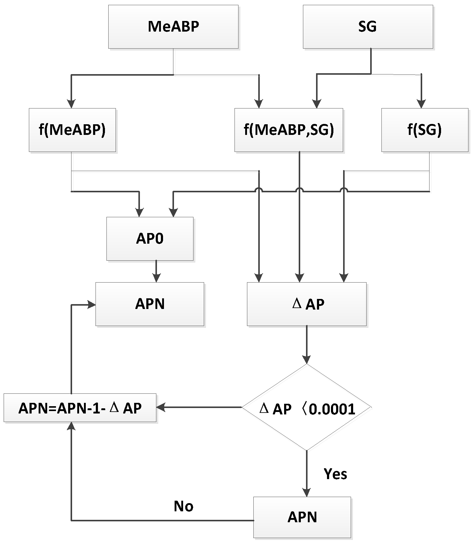
3.2. Application of New Algorithm

A calculation flow chart for the new AP estimation algorithm is presented in Figure 2. The estimation steps are as follows: First, according to the values of the average boiling point and specific gravity, Equations (18), (19), and (21) are applied to calculate f(MeABP), g(SG), and h(MeABP, SG), respectively. Thereafter, the calculated value of the previous step is incorporated into Equation (20) to obtain the initial value required for the iteration, and the iterative calculation is started. Finally, when the iterative condition is judged to converge, the calculation ends, and the estimation result is the output.

The method has a medium average boiling point of approximately 63.33 °C to 593.33 °C and a specific gravity of approximately 0.65 to 1.08. The measurement results are more accurate, and the requirements of most real oil measurements can be met.

3.3. Cross-Validation

As is shown in Equations (18), (19), and (22)–(25), the models presented in this paper involve 21 parameters. To facilitate differentiation, these parameters are named by different variables. The names of the parameters, source formula, and standard values in the equations are shown in

Table 2. Names of model parameters, source formulas, and standard values.

Parameter Name	Source Formula	Standard Value
M0	Equation (18)	−19.15
M1	Equation (18)	0.3145
M2	Equation (18)	−2.289 × 10−4
M3	Equation (18)	7.861 × 10−8
M4	Equation (18)	5.390 × 10−11
M5	Equation (18)	−4.165 × 10−14
S0	Equation (19)	421.5
S1	Equation (19)	−908.8
S2	Equation (19)	879.6
S3	Equation (19)	−479.8
S4	Equation (19)	103.6
S5	Equation (19)	1.87
K1_1	Equation (22)	0.9181
K1_2	Equation (22)	1
K1_3	Equation (22)	−133.5
K2_1	Equation (23)	−1.262 × 10−5
K2_2	Equation (23)	4.269 × 10−4
K3_1	Equation (24)	1.367 × 10−7
K3_2	Equation (24)	4.000 × 10−6
K4_1	Equation (25)	1.170 × 10−3
K4_2	Equation (25)	0.1708

.

In order to verify the stability of the obtained model parameters, we cross-validated the parameters obtained using 142 datapoints. We randomly divided 142 datapoints into 10 groups (where 8 groups contained 14 datapoints and 2 groups contained 15 datapoints). We selected 9 groups as the training set and used the remaining group as the verification set for model validation. through this method, we could obtain 10 training/verification sets. In each experiment, the training set was used to train the parameters of the model, and the ARD of the obtained model was evaluated using the validation set. In addition, in order to prevent instability in random grouping stages, we repeated the experiment 21 times, that is, a total of 21 × 10 = 210 cross-validation experiments. We recorded the model parameters obtained in each experiment and the corresponding average error. For display convenience, we solved the average value of the parameters and the relative error in 30 cross-validation experiments. The results are shown in

Table 3. ARD table corresponding to the mean value of the model parameters obtained with the cross-validation experiment.

N	1	2	3	4	5	6	7	Average
M0	−19.02	−19.23	−19.11	−19.15	−19.21	−19.26	−19.16	−19.163
M1	0.3181	0.3122	0.3147	0.3145	0.3156	0.3135	0.3122	0.31440
M2	−2.24 × 10−4	−2.27 × 10−4	−2.29 × 10−4	−2.28 × 10−4	−2.28 × 10−4	−2.34 × 10−4	−2.27 × 10−4	−2.28 × 10−4
M3	7.91 × 10−8	7.94 × 10−8	7.91 × 10−8	7.87 × 10−8	7.95 × 10−8	7.98 × 10−8	7.88 × 10−8	7.920 × 10−8
M4	5.39 × 10−11	5.39 × 10−11	5.49 × 10−11	5.38 × 10−11	5.37 × 10−11	5.38 × 10−11	5.42 × 10−11	5.403 × 10−11
M5	−3.96 × 10−14	−4.12 × 10−14	−4.17 × 10−14	−4.16 × 10−14	−4.16 × 10−14	−4.15 × 10−14	−4.17 × 10−14	−4.127 × 10−14
S0	421.1	422.1	421.1	421.7	420.9	421.5	421.5	421.41
S1	−911.2	−908.4	−910.2	−909.1	−909.2	−908.3	−907.1	−909.05
S2	880.6	877.6	880.7	880.1	880.2	879.1	879.5	879.67
S3	−479.1	−479.7	−479.8	−479.8	−479.5	−480.1	−479.9	−479.70
S4	104.1	104.2	103.6	103.6	103.7	103.6	103.6	103.77
S5	1.855	1.867	1.861	1.875	1.866	1.876	1.856	1.8656
K1_1	0.9180	0.9121	0.9083	0.9182	0.9151	0.9204	0.9167	0.91554
K1_2	0.9802	0.9995	0.9994	1.000	1.000	1.014	0.9887	0.99740
K1_3	−132.5	−133.5	−132.5	−132.5	−132.5	−132.5	−132.5	−132.64
K2_1	−1.32 × 10−5	−1.27 × 10−5	−1.25 × 10−5	−1.262× 10−5	−1.264 × 10−5	−1.283 × 10−5	−1.241 × 10−5	−1.270 × 10−5
K2_2	4.289 × 10−4	4.267 × 10−4	4.269 × 10−4	4.272 × 10−4	4.271 × 10−4	4.312 × 10−4	4.288 × 10−4	4.2811 × 10−4
K3_1	1.357× 10−7	1.352 × 10−7	1.377 × 10−7	1.370 × 10−7	1.367 × 10−7	1.351 × 10−7	1.347 × 10−7	1.3601 × 10−7
K3_2	3.979× 10−6	4.002 × 10−6	3.979 × 10−6	4.009 × 10−6	4.009 × 10−6	4.001 × 10−6	4.101 × 10−6	4.0114 × 10−6
K4_1	1.163 × 10−3	1.165 × 10−3	1.177 × 10−3	1.172 × 10−3	1.210 × 10−3	1.162 × 10−3	1.165 × 10−3	1.1734 × 10−3
K4_2	0.1709	0.1801	0.1652	0.1633	0.1723	0.1710	0.1722	0.17071
ARD	0.01012	0.00618	0.00749	0.00881	0.00545	0.00449	0.00960	0.00274

.

It can be seen from Table 3 that under the cross-validation test, the models obtained through training with partial datasets could also have high accuracy, and the ARD was basically less than 1%. In addition, we also compared the average value of the parameters obtained with 210 crossover experiments to the standard parameters of the proposed model. The results showed that the deviation of 21 parameters was also within 1%, which proved that the model parameters obtained by the 142 datapoints had high stability.

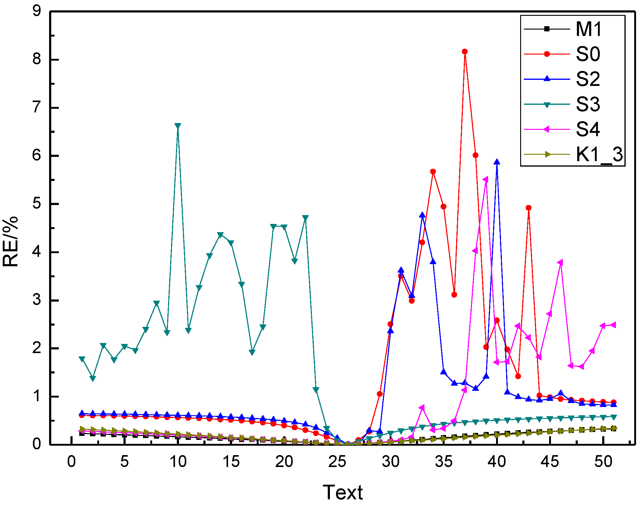
3.4. Parameter Sensitivity Analysis

Parameter sensitivity is a good measure of the stability of an algorithm. In this section, we performed a sensitivity analysis of the 21 parameters in the proposed model. The sensitive parameters in the model could be obtained by evaluating the decline in the accuracy of the model with changing parameters. To further understand the sensitivity of the parameters, the sensitivity range of the sensitive parameters was determined.

3.4.1. Sensitivity Analysis of Individual Parameters

We analyzed 21 parameters in the proposed model one by one. On the basis of the standard values of the model parameters, the tested parameter was changed in each experiment, and the other 20 parameters were fixed. We used a normal distribution to sample new values of the tested parameter. The mean of the normal distribution was the standard value of the parameter, and the standard deviation was 0.2 times the parameter. For example, for a parameter with a standard value of X, the normal distribution was ~N(X, 0.2X). Random sampling was performed within this normal distribution to obtain new model parameters. We used a normal distribution to sample new values of the tested parameter, and the relative errors were counted. In order to prevent large deviations in the random sampling process, we performed 20 experiments on each parameter, sampling 20 new parameters within the normal distribution of the tested parameters. The relative error of the 20 models with the new parameters was estimated, and the ARD was calculated, which was a good index of the sensitivity of the parameter. The results are shown in

Table 4. Sensitivity analysis of 21 parameters in the model.

Parameters	M0	M1	M2	M3	M4	M5	S0
ARD	0.012718	0.11784	0.045702	0.008102	0.003569	0.003712	1.707076
Parameters	S1	S2	S3	S4	S5	K1_1	K1_2
ARD	0.018394	2.110738	1.558631	3.229368	0.002512	0.056777	0.059139
Parameters	K1_3	K2_1	K2_2	K3_1	K3_2	K4_1	K4_2
ARD	0.122109	0.010831	0.004586	0.003963	0.001617	0.00787	0.016993

.

It can be seen from Table 4 that the ARD of the parameters M1 and K1_3 reached more than 10% under this test condition, which indicates that a little variation in the parameter involved a certain impact on the accuracy of the model; therefore, the parameter sensitivity of M1 and K1_3 was high. For the parameters S0, S2, S3, and S4, the ARD even reached more than 150%, which indicates that these four parameters were extremely sensitive, and slight changes could cause large errors. The ARDs of the other 15 parameters were less than 6%. The changes in the parameters had little effect on the accuracy of the model, and the sensitivity of the parameters was low. The experimental results showed that among the 21 parameters of the proposed model, six parameters (M1, K1_3, S0, S2, S3, and S4) were sensitive, and the sensitivity of S0, S2, S3, and S4 was extremely high for the aniline point prediction performed by this model. An adjustment of these parameters should be carefully considered.

3.4.2. Estimation of the Sensitive Range of Sensitive Parameters

In order to have a deep recognition of the sensitivity of the model parameters, we analyzed the sensitivity range of the sensitive parameters obtained in Section 3.4.1. In this experiment, the tested parameter variation range was set at ±50% of the standard value (50%–150% of the standard value). The changing step was set at 2%, that is, 51 experiments were performed for each sensitive parameter. As with the experiments in Section 3.4.1, we estimated 142 datapoints using the model (with the changed parameters) and counted the ARDs of each experiment. The ARDs of each sensitive parameter at different variation ratios are shown in Figure 3.

It can be seen from Figure 3 that for M1 and K1_3, as the parameters gradually moved away from the true value, the ARD also gradually increased. When the parameter change rate was within ±15%, the ARD was less than 10%. Outside this range, the error was greater than 10%. When the rate of change reached 40% or more, the ARD reached 20%. Although these two parameters were more sensitive, as the proportion of parameter changes gradually increased, the ARD growth was also relatively stable. For parameter S3, when the parameter variation range was in the range of −2% to 6%, the ARD was less than 10%, and when the variation was above 6%, the ARD gradually increased, and the change speed was significantly higher than in M1 and K1_3. When the change was less than −2%, the ARD increased rapidly and reached more than 100% at -6%. For parameter S4, when the variation range was in the range of -16% to 10%, the ARD was less than 10%. When the variation was less than −16%, the ARD gradually increased, and the rate of change was similar to that of M1 and K1_3. When the change was greater than 10%, the ARD increased rapidly, and when the rate of change reached 24% or more, the ARD exceeded 100%. For the parameter S0, when the variation range was within ±2%, the ARD was less than 10%. When the variation was less than −2%, the ARD gradually increased, and the change speed was significantly higher than that of the two parameters M1 and K1_3. When the change was greater than 2%, the ARD increased rapidly, and above 6%, the error reached 100% or more. The condition of parameter S2 was close to S0. When the variation range was within ±2%, the ARD was less than 10%. When the variation was less than −2%, the ARD gradually increased, and the variation was similar to S0. When it was greater than 2%, the ARD increased rapidly, and at 8%, the error reached 100% or more. The above results show that the four parameters S0, S2, S3, and S4 were very sensitive and had different sensitivity ranges. When M1 and K1_3 increased and decreased, the relative error changed slowly. The parameter S3 was more sensitive when it was small, and the parameters S0, S2, and S4 were more sensitive when they became larger. Therefore, when using this formula for aniline point estimation, negative adjustments should be avoided for S3, and positive adjustments should be avoided for S0, S2, and S4.

3.5. Data Source Evaluation

The data used for the evaluation in this study consisted of two parts, some of which were from an oil- and gas-related manual [7,23,24,25] that collects a dataset on crude oil analysis and specifications of petroleum products globally to provide an assessment of algorithm accuracy (and therefore serves as an important reference). The other part was composed of actual measured oil data, including Tarim oil (from the literature [3]), Dagang oil, Shengli oil, Renqiu oil, Yangsanmu oil, Daqing oil, and Gudao oil [7,15,16], as well as data on 44 oils collected through actual processes. The data on the oil products of the AP were as follows: aviation coal, catalytic hydrogenation, diesel hydrogenation, catalytic cracking, and atmospheric and vacuum reduction.

The specific gravity and medium average boiling point data of 127 petroleum fractions were selected for this study. The 127 data points used for verification can be recorded in detail in Appendix A,

Table A2. Summary of 127 oil datapoints measured and used to validate the model.

Oil Source	Average Boiling Point (K)	Specific Gravity (15.5 °C)	Aniline Point Experimental Value (K)	Average Boiling Point (K)	Specific Gravity (15.5 °C)	Aniline Point Experimental Value (K)
Tarim [3]	309.15	0.6375	330.25	535.65	0.8358	347.13
	335.65	0.6674	337.83	553.15	0.8393	348.85
	360.65	0.702	333.35	560.65	0.8486	350.85
	367.05	0.7018	334.23	585.65	0.8645	352.35
	385.65	0.728	330.45	610.65	0.8755	353.95
	406.85	0.7365	342.5	635.65	0.8835	358.37
	410.65	0.7526	326.4	660.65	0.8946	361.27
	435.65	0.7701	327.95	685.65	0.902	362.15
	460.65	0.7834	334.6	694.15	0.9118	353.15
	485.65	0.8024	339.65	710.65	0.9062	362.15
	510.75	0.8172	344.3	735.65	0.9119	364.77
	534.35	0.831	347.2	760.65	0.9196	365.2
Dagang [16]	331.95	0.7112	326.55	603.15	0.8767	350.00
	403.15	0.7584	320.40	663.15	0.8860	362.28
	483.15	0.8236	327.60	703.15	0.8928	367.15
	533.15	0.8586	338.25
Shengli [7]	368.15	0.7345	322.65	538.15	0.8298	345.52
	458.15	0.7956	328.10	618.15	0.8508	362.10
	473.15	0.8073	332.12	668.15	0.8691	368.95
Renqiu [7]	403.15	0.7495	333.65	573.15	0.8132	360.51
	493.15	0.8100	341.51	663.15	0.8418	372.06
	533.15	0.8118	348.89	723.15	0.8968	373.29
Yangsanmu [7]	427.15	0.8243	322.08	583.15	0.9062	327.56
	483.15	0.8504	322.46	643.15	0.9295	333.74
	543.15	0.883	325.56	703.15	0.9434	351.42
Daqing [7]	348.15	0.6931	329.35	578.15	0.8271	359.65
	418.15	0.7509	332.25	648.15	0.8399	372.25
	478.15	0.7888	339.05	698.15	0.8489	377.25
Gudao [7]	463.15	0.8278	320.25	653.15	0.9306	340.38
	473.15	0.9484	320.80	708.15	0.9356	356.75
	563.15	0.8912	330.45	743.15	0.9456	362.00
	623.15	0.9211	335.30
Unknown source of petroleum fraction	451.65	0.7784	337.15	572.75	0.8774	339.95
	457.05	0.7950	333.55	660.45	0.8467	374.65
	457.55	0.7858	332.55	663.35	0.8505	373.55
	457.75	0.7846	332.65	665.85	0.8617	369.35
	459.05	0.8092	324.85	666.45	0.9045	350.15
	459.15	0.7723	341.15	666.45	0.9073	353.15
	459.25	0.7804	338.65	667.05	0.8761	366.45
	459.35	0.7902	329.95	667.35	0.8921	356.65
	459.75	0.8052	330.95	667.55	0.9292	342.05
	459.85	0.8071	329.35	668.65	0.8641	371.65
	462.95	0.8043	331.55	672.45	0.9028	351.15
	463.35	0.8260	322.05	672.65	0.9020	353.25
	463.95	0.8165	325.15	672.95	0.8989	360.55
	466.15	0.7895	338.75	673.05	0.8528	375.65
	468.85	0.8073	331.35	673.15	0.8880	361.85
	471.15	0.8005	334.45	674.55	0.8607	372.15
	471.35	0.7966	337.05	707.15	0.9231	351.15
	542.05	0.8189	355.35	719.05	0.8813	377.55
	549.85	0.8368	349.75	720.65	0.8869	376.85
	552.15	0.8477	342.95	726.95	0.9247	357.95
	552.25	0.8169	357.15	728.35	0.8711	382.65
	555.15	0.8505	346.15	728.65	0.9139	360.55
	556.55	0.8276	356.05	731.35	0.8894	376.85
	557.85	0.8517	341.15	737.65	0.8763	383.15
	557.85	0.8440	346.75	739.45	0.8776	381.95
	558.45	0.8566	346.15	740.05	0.9267	365.75
	561.35	0.8404	350.95	742.55	0.8949	376.75
	562.65	0.8370	353.45	744.15	0.9593	350.35
	564.05	0.8702	335.05	745.25	0.9385	356.55
	564.55	0.8847	333.25	746.35	0.9140	368.15
	566.45	0.8526	344.45	746.35	0.9099	369.05
	567.65	0.8351	354.95	746.65	0.9354	354.15
	567.95	0.8744	338.45

. The petroleum fraction was obtained through the distillation of crude oil through a real boiling point curve, covering various types of crude oil and its fractions both locally and globally. The AP of each oil was predicted by the new algorithm, and the results and relative deviations were analyzed.

4. Evaluation Results of New AP Algorithm

4.1. Evaluation Results of New Algorithm

The petroleum fraction used in the model verification had a specific gravity ranging from 0.65 to 1.10, and the average boiling point range was 300.48–866.48 K. A scatterplot of the predicted values using the new algorithm and the actual values of the AP is presented in Figure 4.

It can be observed from the figure that the distribution of the predicted and actual values of the oil was similar to the straight line y = x; that is, the predicted value of the oil was approximately equal to the true value. The proposed new algorithm exhibited an estimated relative deviation of more than 90% of the actual oil AP (less than 0.5%), an ARD of 0.17% for all oils, and a maximum relative deviation (MRD) of 0.634%. It could be proven that the proposed AP estimation algorithm provided higher accuracy in estimating the AP of the oil substances used in the test.

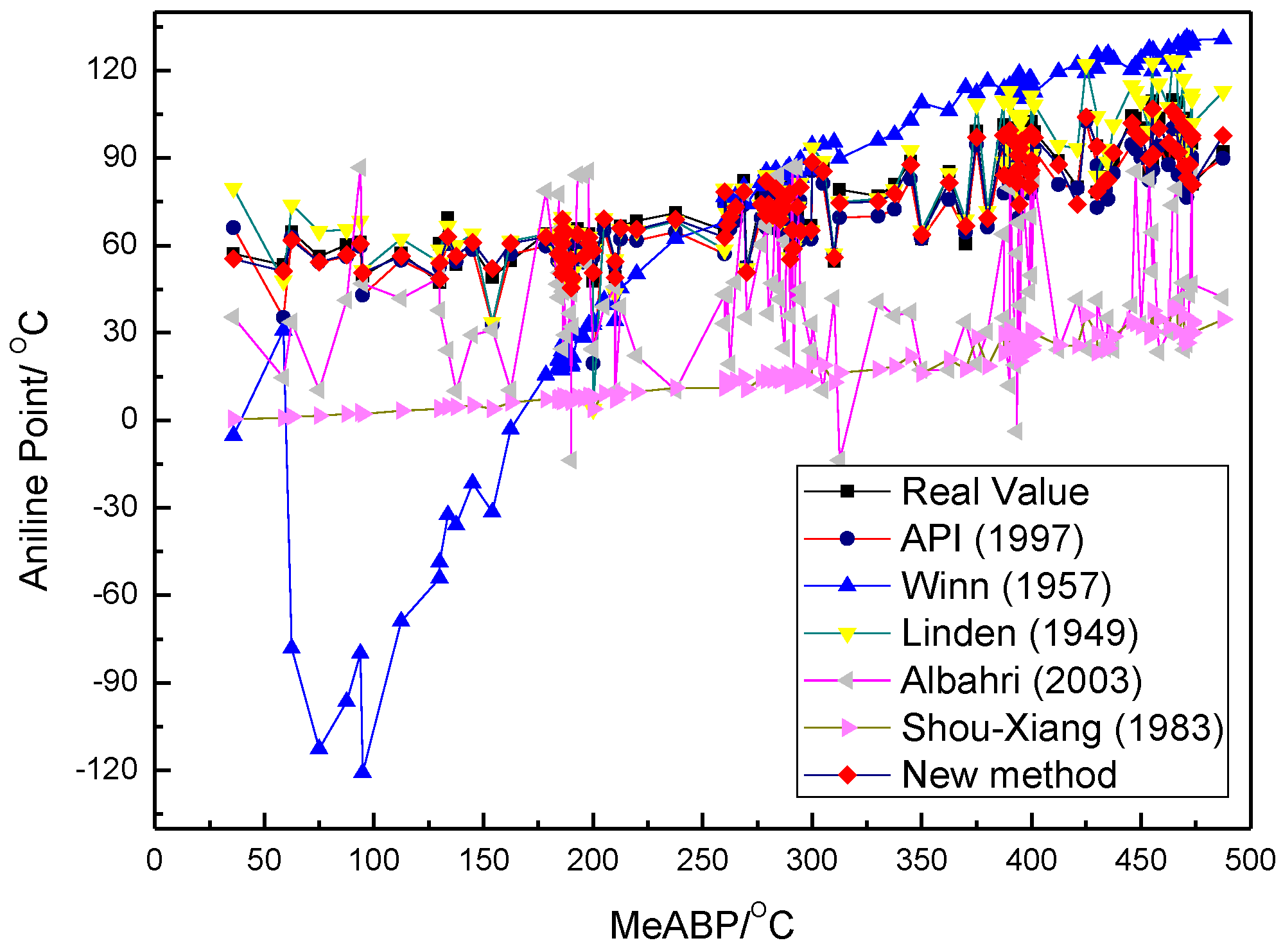
4.2. Comparison of New Algorithm and Common Models

The test results are illustrated in Figure 5.

As is indicated in Figure 5, the Winn method had a relatively large relative deviation, while the three methods with small deviations were the newly proposed method, the Shoudeqing method, and the API method. The estimated and measured values of each method were compared, as is illustrated in Figure 6.

According to Figure 5 and Figure 6, as the measured value of the petroleum fraction gradually increased, the trend of the Shoudeqing method became consistent with the measured value, but a large deviation occurred. The predicted values of the Albahri and Chen–Xionghua methods fluctuated significantly. In the Linden method, a higher average boiling point temperature resulted in a larger deviation. The Winn method exhibited a larger deviation in the average boiling point range below 200 °C. The new algorithm exhibited less deviation in the predicted value of the petroleum fraction used for verification. The statistics on the estimated deviations of each method are presented in

Table 5. Relative deviation distribution of AP estimation results of petroleum fractions.

The Relative Error Range (%)	Number
	API	Winn	Linden	Walsh–Mortimer	Albahri	Chen	Shou	New Method
≤5%	47	7	55	6	6	13	6	96
5%–10%	59	9	33	5	4	5	21	28
10%–20%	18	25	34	11	13	2	41	3
≥20%	3	86	5	105	104	104	59	0

.

In terms of the deviation distribution, the relative deviation of the new AP estimation algorithm for 96 oil test results was less than 5%, while the other methods only yielded 55 oils with AP estimation results with a relative deviation of less than 5%. The new AP estimation algorithm significantly reduced the AP estimation bias. Moreover, the AAD, ARD, maximum absolute deviation (MAD), and MRD of the test results were calculated. The results are displayed in

Table 6. Comparison of AP estimation results of petroleum fractions. MAD: maximum absolute deviation; MRD: maximum relative deviation.

Method	N	AAD (°C)	ARD (%)	MAD (°C)	MRD (%)
API	127	5.17	7.01	28.14	59.05
Winn	127	34.37	32.61	70.30	44.03
Linden	127	6.38	8.46	43.80	51.92
Walsh–Mortimer	127	37.73	28.8	43.83	52.92
Albahri	127	35.36	47.48	46.18	59.38
Chen	127	40.30	44.71	47.53	59.00
Shou	127	57.74	18.70	72.08	28.54
New method	127	2.58	3.55	6.98	10.90

.

As is indicated in Table 6, the ARDs of the API, Winn, Walsh–Mortimer, Linden, Albahari, Chen–Xionghua, and Shoudeqing methods were all above 5%. Moreover, the smallest deviation of the API method reached 7.01%. The ARD of the new AP estimation algorithm was approximately 3.55%, which was roughly two times lower than the estimated deviation of the existing models, indicating that the proposed method could effectively improve the AP estimation accuracy.

In summary, the proposed AP estimation algorithm exhibited higher accuracy and provided a greater improvement than the commonly used algorithms did. In terms of model adaptability, the API and Albahri methods yielded a relatively accurate prediction value when the average boiling point ranged from 320.48 to 580.48 K and the specific gravity ranged from 0.75 to 0.90. In particular, for the API algorithm, the ARD between the predicted and measured values of the AP was 5.33% for datapoints with an average boiling point less than 672.04 K. For datapoints with a medium average boiling point greater than 672.04 K, the ARD between the predicted and measured values was 10.08%; therefore, this method is not applicable when calculating the average boiling point of hydrocarbon compounds or the APs of petroleum fractions greater than 672.04 K. The proposed AP estimation algorithm had a moderate average boiling point of approximately 336.48−866.48 K, and the specific gravity was approximately 0.65 to 1.08. The prediction results were more accurate and offered a wider application range than those of the other algorithms. Therefore, the proposed AP estimation method provides higher accuracy and greater stability, as well as wider applicability.

5. Conclusions

Seven classical AP estimation methods, including the API and Winn methods, were summarized and evaluated. A new AP estimation algorithm was proposed. Through verification of the new method and a comparison to the original methods, the following conclusions could be obtained:

(1)

Using experimental data, AP estimation tests were carried out on the seven methods. The results demonstrated that these algorithms generally exhibited large deviations in the calculation of APs. The accuracy of the API method was slightly higher than those of the other six methods, but the ARD of the AP calculation of the petroleum fraction was more than 5%. The reasons for the inaccurate calculations of the original methods were analyzed and were mainly determined to be a lack of original data, simple models, simple regression methods, and no postprocessing;

(2)

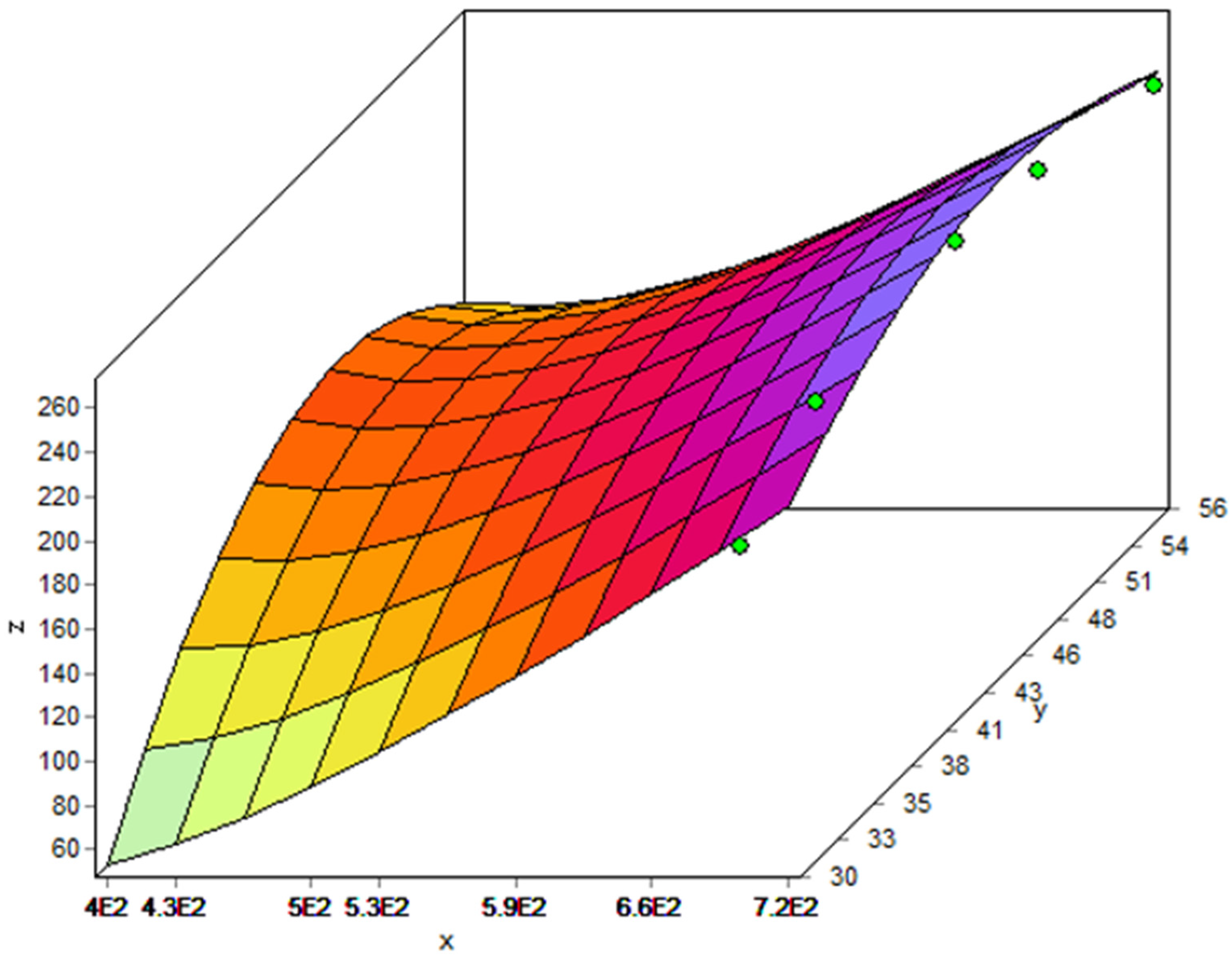
Using multiple linear regression, the average boiling point and specific gravity were taken as the main structural parameters. A new algorithm for the AP of petroleum fractions was developed by means of data regression and iterative correction. The superiority of this method compared to the original methods was confirmed, as it uses a wider range of experimental data to obtain a new correlation;

(3)

When comparing the estimation results of APs by different models, the ARD of the new algorithm was 3.55% and the MRD was less than 7%. Compared to the best existing estimation model, the AP model estimated that the ARD would be reduced by approximately twice the initial ARD and that the MRD would be reduced by approximately six times the initial ARD.

In summary, the new algorithm for the petroleum fraction AP offers significant value, both as a theoretical algorithm and for actual oil prediction. The objective function regression–iteration correction method not only offers application potential in the estimation of petroleum fraction APs, but also provides a solid reference for other hydrocarbon material properties.

References

1. Gharagheizi, F.; Tirandazi, B.; Barzin, R. Estimation of Aniline Point Temperature of Pure Hydrocarbons: A Quantitative Structure−Property Relationship Approach. Ind. Eng. Chem. Res. 2009, 48, 1678–1682. [Google Scholar] [CrossRef]
2. Guo, Y.G. Determination and Correlation of Electrochemical Oil Aniline Point. Lubr. Fuels 2016, z1, 30–31. [Google Scholar]
3. Jiang, H.Q. Prediction of the Physical Properties of Tarim Distillate Oil; China University of Petroleum: Beijing, China, 2010; pp. 58–67. [Google Scholar]
4. GB/T 262-2010. Determination of Aniline Point and Mixed Aniline Point in Petroleum Products and Hydrocarbon Solvents; Chemical Industry Press: Beijing, China, 1964; pp. 301–304. Available online: https://www.antpedia.com/standard/6159574.html (accessed on 10 September 2019).
5. Gharagheizi, F. QSPR analysis for intrinsic viscosity of polymer solutions by means of GA-MLR and RBFNN. Comput. Mater. Sci. 2007, 40, 159–167. [Google Scholar] [CrossRef]
6. Zhang, Y.Y. Prediction of aniline point of hydrocarbons based on QSPR method. J. Saf. Environ. 2015, 06, 126–131. [Google Scholar] [CrossRef] [PubMed]
7. Shou, D.Q. Study on the Basic Properties of Petroleum in China (I)—Determination and Correlation of Average Molecular Weight of Petroleum Straight Distillate. J. East China Pet. Univ. 1983, 03, 334–342. [Google Scholar]
8. Albahri, T. Specific Gravity, RVP, Octane Number, and Saturates, Olefins, and Aromatics Fractional Composition of Gasoline and Petroleum Fractions by Neural Network Algorithms. Pet. Sci. Technol. 2014, 32–35. [Google Scholar] [CrossRef]
9. Riazi, M.R. Characterization and Properties of Petroleum Fractions; Hydrocarbon Process: Washington, DC, USA, 1999; pp. 137–138. [Google Scholar]
10. American Petroleum Institute. Technical Data Book Petroleum Refining, 6th ed.; American Petroleum Institute: Washington, DC, USA, 1997; pp. 356–368. [Google Scholar]
11. Winn, E.W. Physical Properties by Nomogram. Pet. Refin. 1957, 36, 157–159. [Google Scholar]
12. Linden, H.R. The Relationship of Physical Properties and Ultimate Analysis of Liquid Hydrocarbon. Oil Gas J. 1949, 48, 60–65. [Google Scholar]
13. Walsh, R.E. New Way to Test Product Quality. Hydrocarb. Process. 1971, 50, 153–158. [Google Scholar]
14. Albahri, T.A.; Riazi, M.R.; Alqattan, A.A. Analysis of Quality of the Petroleum Fuels. Energy Fuels 2003, 17, 689–693. [Google Scholar] [CrossRef]
15. Chen, X.H.; Li, L. A new mathematical correlation of aniline points in petroleum fractions. Guangdong J. Chem. Eng. 2019, 08, 57–58. [Google Scholar] [CrossRef]
16. Shou, D.Q. Research on the Basic Properties of Petroleum in China (I). Pet. Refin. Chem. Eng. 1984, 04, 1–8. [Google Scholar]
17. Yin, C.S.; Liu, X.H.; Guo, W.M.; Liu, S.S.; Han, S.K.; Wang, L.S. Multi-objective modeling and assessment of partition properties: A GA-based quantitative structure-property relationship approach. Chin. J. Chem. 2003, 21, 1150–1158. [Google Scholar] [CrossRef]
18. Jenkins, G.I. Quick Measure of Jet Fuel Properties. Hydrocarb. Process. 1968, 47, 161–164. [Google Scholar]
19. Riazi, M.; Albahri, T.; Alqattan, A. Prediction of Reid Vapor Pressure of Petroleum Fuels. Pet. Sci. Technol. 2005, 23, 75–86. [Google Scholar] [CrossRef]
20. Gary, J.H.; Handwerk, G.E.; Kaiser, M.J. Petroleum Refining: Technology and Economics[M]; CRC Press: Boca Raton, FL, USA, 2007. [Google Scholar]
21. Li, W. Research on Small Sample Multivariate Experimental Design and Optimization Analysis System; Wuhan University of Technology: Wuhan, China, 2012; pp. 4–8. [Google Scholar]
22. Xiao, S.J.; Zhu, X.F. An Improved Fast and Efficient Differential Evolution Algorithm. J. Hefei Univ. Technol. Nat. Sci. 2009, 32, 1700–1703. [Google Scholar]
23. Albahri, T.A. Prediction of the aniline point temperature of pure hydrocarbon liquids and their mixtures from molecular structure. J. Mol. Liq. 2012, 174, 80–85. [Google Scholar] [CrossRef]
24. Carl, L.Y. Thermophysical Properties of Chemicals and Hydrocarbons [M]; William Andrew Publishing: New York, NY, USA, 2008; p. 802. [Google Scholar]
25. Speight, J.G. The Chemistry and Technology of Coal, 2nd ed.; CRC Press: Boca Raton, FL, USA, 1983; Volume 36, pp. 170–172. [Google Scholar]
Figure 1. Molecular weight and characteristic factors of the petroleum fractions proposed by Winn.
Processes 07 00912 g001
Figure 2. Proposed new model calculation flow chart.
Processes 07 00912 g002
Figure 3. ARDs of the six sensitive parameters (M1, S0, S2, S3, S4, and K1_3) at varying ratios.
Processes 07 00912 g003
Figure 4. Contrastive analysis chart of predicted and real oil products.
Processes 07 00912 g004
Figure 5. Error distributions of different methods and real values.
Processes 07 00912 g005
Figure 6. Trend charts of results for different methods and real values.
Processes 07 00912 g006