Abstract
Aiming at addressing the problem that the faults in axial piston pumps are complex and difficult to effectively diagnose, an axial piston pump fault diagnosis method that is based on the combination of Mel-frequency cepstrum coefficients (MFCC) and the extreme learning machine (ELM) is proposed. Firstly, a sound sensor is used to realize contactless sound signal acquisition of the axial piston pump. The wavelet packet default threshold denoises the original acquired sound signals. Afterwards, windowing and framing are added to the de-noised sound signals. The MFCC voiceprint characteristics of the processed sound signals are extracted. The voiceprint characteristics are divided into a training sample set and test sample set. ELM models with different numbers of neurons in the hidden layers are established for training and testing. The relationship between the number of neurons in the hidden layer and the recognition accuracy rate is obtained. The ELM model with the optimal number of hidden layer neurons is established and trained with the training sample set. The trained ELM model is applied to the test sample set for fault diagnosis. The fault diagnosis results are obtained. The fault diagnosis results of the ELM model are compared with those of the back propagation (BP) neural network and the support vector machine. The results show that the fault diagnosis method that is proposed in this paper has a higher recognition accuracy rate, shorter training and diagnosis times, and better application prospect.
1. Introduction
Hydraulic systems are highly nonlinear systems [1]. Circuits are coupled with each other. As a result, performance degradation and fault mechanisms are complex and varied. Hydraulic systems transmit power through hydraulic oil. The system parameters are difficult to effectively observe and the fault information is difficult to obtain. Therefore, fault diagnosis of hydraulic systems is difficult.
In recent years, hydraulic systems have been developing in the direction of lightweight, small volume, high-pressure, high power density, and variable pressure characteristics [2]. The complexity and automation level of hydraulic systems have been continuously improving [3]. As the heart of the hydraulic system, the running state of the hydraulic pump will directly affect the working state of the entire hydraulic system and even the industrial equipment as a whole. Therefore, it is particularly important to conduct status monitoring and diagnosis [4,5,6,7]. The failure forms of the axial piston mainly pump include loose slipper, slipper wear, swash plate wear, center spring failure, etc. Monitoring the working state of the hydraulic pump and the accurate diagnosis of fault types cannot only guide maintenance personnel to achieve timely repair, but can also improve the production efficiency and reduce production costs.
The traditional fault diagnosis method of hydraulic systems mainly relies on the rich working experience of maintenance personnel [8]. The identification accuracy of hydraulic systems is low by means of sensory diagnosis, oil sample analysis, and fault tree analysis. With the development of signal processing technology, computer technology, and control theory, the fault diagnosis theory of hydraulic systems is rapidly developing. Some advanced fault diagnosis methods have been successively applied to the fault diagnosis of hydraulic pumps. Relatively ideal fault diagnosis results have been obtained. For example, Wang et al. [9] proposed a variety of fault pattern recognition methods for hydraulic pumps based on the neural network, and achieved satisfactory results in terms of diagnosis and identification; Jiang et al. [10] proposed that the correlation dimension analysis method could effectively monitor the working status of a hydraulic pump and diagnose the occurrence of faults; Wang et al. [11] proposed that the wavelet de-noising method could effectively improve the characteristics of the weak fault signal of the hydraulic pump, so as to improve the fault diagnosis effect; Peng et al. [12] proposed a fault diagnosis method for the hydraulic pump that was based on the neural network method, which could significantly shorten the training time of the model; and, Tang et al. [13] proposed a fault diagnosis method for the hydraulic pump based on empirical mode decomposition (EMD) envelope spectrum analysis, which could effectively extract the fault characteristics of the hydraulic pump early in the morning and accurately realize the fault diagnosis of the hydraulic pump [14].
The traditional fault diagnosis method mainly relies on installing a vibration sensor on the equipment to extract fault information regarding the equipment [15]. However, it is difficult to install the sensor due to the limitation of the installation space of some equipment. This paper proposes to extract the state information of the equipment by monitoring the sound signals around the equipment to avoid the complicated installation process of traditional contact sensors in order to solve this problem. The contactless sensor is easy to install and operate and it is more suitable for industrial use.
Sound signals are important carriers of information. Sound has a strong diffraction ability and it is easy to collect when compared with other signals [16]. With the development of Mel-frequency cepstrum coefficients (MFCC) feature extraction and other theories, there have been breakthroughs in speech recognition and other fields [17]. Zhu Yu et al. applied MFCC to effectively identify the void under concrete pavement slabs [18]. Liu Sisi et al. used MFCC to effectively identify the existence of abnormal noise in the car window motor [19].
The single hidden layer feedforward neural network has good learning ability. It has been widely used in many fields. As the feedforward neural network mostly adopts the gradient descent algorithm for training, it has some shortcomings, such as a slow training speed, ease of falling into the local optimal, and sensitivity to the learning rate. With the development of artificial intelligence technology, various intelligent algorithms have been widely applied in the field of fault diagnosis. For example, Jiang et al. [20] applied the variational mode decomposition method and the kernel fuzzy c-means clustering method for rolling bearing fault diagnosis and obtained a fault identification rate of 97.5%; Zheng et al. [21] proposed that the local mean decomposition and generalized morphological fractal dimension should be applied in gear fault diagnosis; Tamilselvan et al. [22] proposed a classification model of aviation engine health based on the deep confidence neural network (DBN); and, Zhao et al. [23] proposed a method of rolling bearing health assessment that was based on stacked denoising auto encoder (SDAE). The extreme learning machine (ELM) is an emerging learning algorithm [24]. This algorithm randomly generates the connection weights between the input layer and the hidden layer and the threshold value of hidden layer neurons. In the training process, the algorithm adjusts itself according to the training samples without manual participation. The unique optimal solution can only be obtained by setting the number of neurons in the hidden layer. It has the advantages of a fast learning speed and strong generalization ability. It is widely used in classification, regression, clustering, feature learning, and other problems. However, it has not been applied to the fault diagnosis of the axial piston pump based on sound signals.
This paper presents a fault diagnosis method for the axial piston pump that is based on the combination of voiceprint characteristics and ELM. Figure 1 shows the diagnosis process. The whole fault diagnosis process is divided into three stages, which are data acquisition and preprocessing, feature learning, and fault diagnosis. Firstly, the fault sound signal of the axial piston pump is collected and denoised by the wavelet packet method. Subsequently, the sound signal after noise elimination is preweighted, and so on. The Mel frequency scale triangular filtering method is used to solve the MFCC voiceprint characteristics of the axial piston pump sound signal. The MFCC is taken as the characteristic vector. Finally, ELM is applied to the feature learning and fault diagnosis of the feature vector.
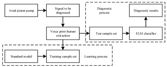
Figure 1.
Fault diagnosis process of the axial piston pump.
2. Voiceprint Characteristics Extraction Method Based on the MFCC
Voiceprint recognition technology is a method that is used to judge a speaker by extracting the features of the voice signal. It establishes the speaker’s feature vector database to determine the identity of the speaker [25]. The sound signals of mechanical equipment contain rich information, which can reflect its own working state and fault condition to a certain extent. Therefore, the voiceprint characteristics identify the sound signal of the axial piston pump. Subsequently, the fault state is accurately diagnosed. It can provide theoretical guidance for the on-condition maintenance of the axial piston pump.
The MFCC is based on the human ear’s non-linear perception of sound. The sensitivity of the human ear to sound varies with frequency, and it is more sensitive to low frequency than high frequency. The sound signal of the axial piston pump has strong nonlinearity and it is non-stationary. In this study, the MFCC was used to extract the voiceprint characteristic information in the sound signal of the axial piston pump. At present, the Mel frequency scale triangular filtering method is commonly used to solve the MFCC features. Figure 2 shows the specific feature extraction process. Firstly, wavelet packet denoising was carried out on the sound signal . Afterwards, the window and frame preprocessing methods were used to denoise the signal . Fast Fourier transform (FFT) was applied to the processed time domain signal . The signal was converted from the time domain to the frequency domain, and the amplitude spectrum was obtained. The amplitude spectrum was passed through the Mel filter bank to obtain the Mel spectrum . The logarithmic energy of each Mel spectrum was calculated. The Discrete Cosine Transform (DCT) was conducted on all to obtain the MFCC.
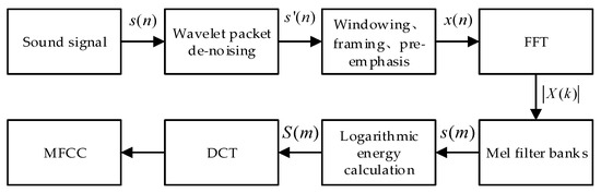
Figure 2.
The extraction process of the Mel-frequency cepstrum coefficient (MFCC) voiceprint characteristics.
2.1. Denoising Method Based on the Wavelet Packet Default Threshold
The wavelet packet threshold denoising method used was as follows. Firstly, an orthogonal wavelet basis was selected. The processing signal was decomposed by K-layer wavelet packet decomposition. An appropriate threshold value was selected for threshold quantization for each decomposed wavelet packet coefficient. Finally, the de-noising signal was obtained by wavelet packet reconstruction.
In the wavelet packet denoising process, the selection of the threshold function is more critical. The commonly used threshold functions have hard threshold and soft threshold functions. For hard threshold methods, the coefficient remains unchanged when the absolute value of wavelet packet decomposition coefficient is greater than the threshold value; otherwise, zero is set. This quantization method is an easy way to make the signal oscillate [26]. Therefore, this study chose the soft threshold processing method.
The hard threshold function is defined as [26].
The soft threshold function is defined as [25]
where is the wavelet packet coefficients after threshold processing. is the original wavelet packet decomposition coefficient. is the threshold value.
2.2. Pre-Emphasis, Windowing, and Framing of the Signal
The purpose of pre-emphasis is to make the energy of the low frequency part and the high frequency part have similar amplitudes. It is necessary to strengthen the high frequency part of the collected sound signal, so that the model can make better use of the high frequency formant, thereby improving the accuracy of recognition. Pre-emphasis is achieved by a first-order high-pass filter, whose frequency domain representation is
where is the coefficient, which is usually 0.97.
As a typical non-stationary signal, the noise signal of the equipment takes F sampling points as an observation unit, which is called a frame. In this paper, a frame is a sample, and the process of framing involves dividing the original signal into p samples. Figure 3 shows the relationship between the frame shift and frame length.
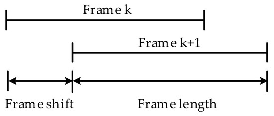
Figure 3.
Relationship between frame shift and frame length.
Each frame is multiplied by a window function to increase the continuity of the left and right signals. Other signals are shielded, also known as short-time signal processing. The sound signal after adding window function is
where is the sound signal after denoising. is the time domain signal for each frame after windowing processing. is the Hamming window function.
2.3. Fast Fourier Transform
It is difficult to identify the signal characteristics in the time domain. When the working state of the axial piston pump changes, the energy distribution of its sound signal in the frequency domain will also change. FFT of the preprocessed sound signal obtains the frequency spectrum of each sample. The discrete Fourier transform of the sound signal is
where is the spectrum of the sound signal. is the number of sampling iterations of the Fourier transform.
2.4. Mel Frequency Filtering
The power spectrum was obtained by taking the squared modulus of the frequency spectrum of the signal and then making it pass through the Mel filter bank to calculate its logarithmic energy.
where is the frequency response of the filter bank. M is the number of the triangle filter.
2.5. Discrete Cosine Transform
DCT was applied to the logarithmic energy of the signal. The Mel-frequency cepstrum coefficient was obtained. The calculation method was as follows:
where is the order of MFCC.
The standard MFCC only reflects the static characteristics of the signal. The first-order difference (ΔMFCC) of the MFCC was introduced for describing the dynamic characteristics of the signal.
ΔMFCC can describe the dynamic characteristics of sound signals and it has good noise robustness. The calculation method used was
where is a constant, generally 2 or 3, which indicates the number of frames participating in the difference operation before and after the current frame. In this study, was assumed to be 2. is the Mel cepstrum coefficient.
3. Extreme Learning Machine Theory
The ELM is a single hidden layer feedforward neural network. Figure 4 shows its network structure. It consists of an input layer, hidden layer, and output layer. There is a full connection between the neurons of the input layer and hidden layer or the hidden layer and output layer. The input layer has n neurons, which correspond to n eigenvalues. The hidden layer has l neurons. The output layer has m neurons, which correspond to the m working states of the axial piston pump.
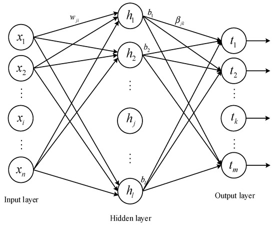
Figure 4.
Network structure of the extreme learning machine (ELM).
The fault sample set is , where X is the input sample matrix and Y is the desired output matrix corresponding to X. p is the number of samples. is the input vector of the j-th sample in X. n is the dimension of the sample. is the j-th expected output vector in Y. m is the dimension of output vector. The activation function of the hidden layer neurons is . The output matrix T of the single hidden layer feedforward neural network with l hidden layer nodes is [27,28].
where, , is the weight vector between the input neurons and the i-th hidden layer neuron, is a weight between the i-th hidden layer neuron and the k-th output layer neuron, the biases of the hidden layer neurons are , and is the bias of the i-th hidden layer neuron.
Equations (9) and (10) can be expressed as
where is the transposition of the output matrix of the neural network and is the hidden layer output matrix of the neural network. The specific form of is [29].
When the number of hidden layer neurons of the single hidden layer feedforward neural network is equal to the number of the training sets p, for any weight matrix and bias vector , the neural network can approach the training samples with zero error [30], which is
However, when the number of training samples p is large, the number of neurons l in the hidden layer is usually smaller than p in order to reduce the computation of the neural network, so the training error of the neural network approaches an arbitrary , that is
Therefore, when the activation function of the hidden layer is infinitely differentiable, the weight matrix and the hidden layer bias of the input layer and the hidden layer can be randomly determined before training and remain unchanged during the training [31]. At this time, the output matrix of the hidden layer is a constant matrix. The connection weight matrix between the hidden layer and the output layer can be obtained by solving the least squares solution of the linear equations , which is
where, is the Moore–Penrose generalized inverse of the output matrix H of the hidden layer.
The learning algorithm of the ELM mainly has the following steps:
- (1)
- Determining the number of hidden neurons. The connection weight matrix between the input layer and the hidden layer and bias vector of hidden layer neurons are randomly set.
- (2)
- Selecting an infinitely differentiable function as the activation function of the hidden layer neurons. Subsequently, the hidden layer output matrix H is calculated [32].
- (3)
- The output layer weight is calculated.
4. Data Acquisition and Fault Feature Extraction
4.1. Axial Piston Pump Fault Simulation Test Bench
Figure 5 shows the fault simulation test bench diagram used in this paper. The vane pump supplies oil to the axial piston pump. The axial piston pump [33] supplies pressurized oil to the system. The test bench can simulate the typical faults of the axial piston pump, such as single plunger slipper wear, single plunger loose slipper, swash plate wear, etc. The testbed meets the requirements of the test verification.
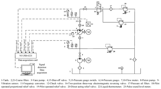
Figure 5.
Hydraulic system diagram of the hydraulic pump fault simulation testbed.
The outlet pressure of the axial piston pump remains unchanged when the working pressure of the overflow valve of the system is adjusted. The rotational speed of the motor determines the rotational speed of the axial piston pump. Meanwhile, the rotational speed of the quantitative pump determines the flow rate of the pump. The outlet pressure, flow rate, and rotational speed of the axial piston pump will not change in the stable working process. Therefore, the change of working environment of the quantitative hydraulic pump with time was not considered in the test process. During the test, the system pressure was set to 10 MPa by pilot type relief valve 19. Table 1 shows the model and performance parameters of the motor, axial piston pump, sensor, and data acquisition card selected for the test bench.

Table 1.
Model and performance parameters of the test elements.
The adopted test bench hydraulic pump installation arrangement was the upper type (horizontal type). This arrangement not only facilitates the disassembly and assembly of the pump, but also facilitates the installation of the sensor [34]. The arrangement of the sensor is shown in Figure 6.
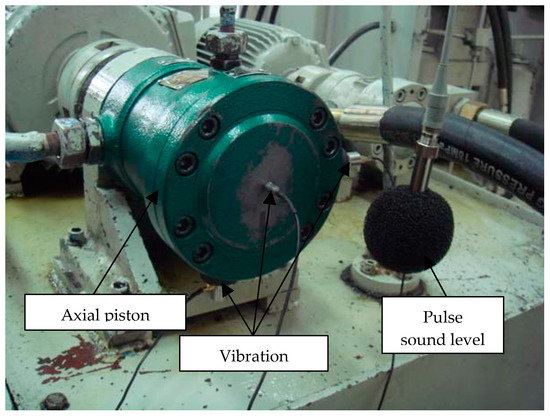
Figure 6.
Hydraulic pump fault simulation test bed.
During the test, sound signals of the pump were collected in four different states, which were the normal working state, single slipper loose fault, single slipper wear fault, and swash plate wear failure.
LabVIEW was used to write the data acquisition program. A USB-6221 data acquisition card that was produced by National Instruments was selected for data acquisition, and 250 kS/s was the highest sampling frequency. During the sampling process, the sampling frequency was set to 20 kHz and the sampling time was set to 15 s. Figure 7 shows the front panel of the acquisition program.
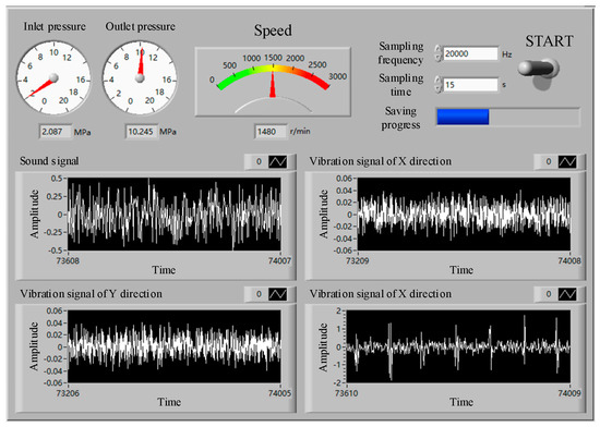
Figure 7.
Front panel of the LabVIEW data acquisition program.
4.2. Feature Extraction of Vibration Signals Based on the MFCC
In the process of collecting sound signals, the collected signals were doped with many noise components due to the influence of environmental noise. The wavelet packet default threshold denoising was first applied to the collected sound signals in order to extract effective information from the sound signals. The method performed noise cancellation. When comparing Figure 8a,b, the method of applying wavelet packet denoising was able to remove the noise component in the original sound signal to some extent. The high-frequency part of the sound signal was pre-emphasized after denoising in order to improve the recognition accuracy. Generally, pre-emphasis is performed for flattening the magnitude spectrum and balancing the high and low frequency components. During the propagation of sound signal, high frequency and low frequency signals will attenuate to different degrees. The model can make better use of the high-frequency formant of the sound signal by accentuating the high-frequency part of the sound and increasing the high frequency amplitude of the sound. Figure 8c shows the time domain diagram of the pre-emphasis of the sound signal of the single slipper wear fault. When comparing Figure 8b with Figure 8c, it can be seen that the emphasis of the original sound signal made the amplitude of the signal smaller.
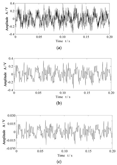
Figure 8.
Time domain diagram of the single slipper wear fault sound signal: (a) Original sound signal; (b) sound signal after wavelet packet denoising by the default threshold; (c) sound signal after denoising and pre-emphasis.
Figure 9 shows the power spectral density, being plotted by the voice signal of the single slipper wear fault. The pre-weighted signal was effectively enhanced in the high frequency part. For example, the signal spectrum values at 5500, 7173, and 8840 Hz were increased by 8.3, 12.17, and 13.37 dB, respectively. At the same time, with the increase of signal frequency, the frequency spectrum value more obviously increased.
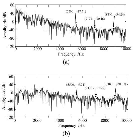
Figure 9.
Power spectral density of the sound signal of the single slipper wear fault: (a) original sound signal; and, (b) sound signal after pre-emphasis.
The enhanced sound signal was windowed and framed, and every 4000 points of the original sound signal were intercepted as one frame, and the frame shift was 25%, which is, 1000 points. 4000 points corresponded to the hydraulic pump rotating about five turns since the pump speed was 1480 r/min. and the sampling frequency was 20 kHz.
FFT was applied to the pre-processed sound signal, which changed from the time domain to the frequency domain, and the signal then passed through the triangular Mel filter bank to obtain the MFCC. The DCT was performed after taking the logarithm. Afterwards, the cepstrum was changed and the MFCC and the first-order difference coefficient(ΔMFCC) were obtained, that is, the 12-dimensional MFCC and the 12-dimensional ΔMFCC together constituted the characteristic parameters of the sound signal. Figure 10 shows the MFCC and the ΔMFCC of one of the training samples. Among them, dimensions 1–12 are the MFCC and dimensions 13–24 are the ΔMFCC.
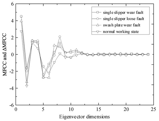
Figure 10.
MFCC and △MFCC of the axial piston pump sound signal.
It can be seen from Figure 10 that the difference of the first 12-dimensional MFCC in the characteristic parameters of the axial piston pump is more obvious, and the latter 12-dimensional ΔMFCC cannot reflect the different working states of the axial piston pump. Therefore, the first 12-dimensional MFCC was selected as the feature vector for the axial piston pump working state in this study. Four working states of the axial piston pump, which is the normal working state, single slipper wear fault, single slipper loose fault, and swash plate wear fault were selected, each of which was 1200 frames, i.e., 1200 samples, of which 1000 samples in each working state were used as a training set and 200 samples were used as a test set.
5. Fault Diagnosis of the Hydraulic Pump Based on ELM
In the training process of ELM, only the number of hidden layer neurons needs to be set to obtain the unique optimal solution. Therefore, 1000 samples of each of the four hydraulic pump states were first selected as training samples and 200 samples of each state were selected as test samples in order to obtain the appropriate number of neurons. Figure 11 shows the relationship between the recognition accuracy and the number of ELM hidden layer neurons. As can be seen from the figure, the recognition accuracy gradually increased with the increase in the number of hidden layer neurons. The number of hidden layer neurons selected in ELM in this study was 15. Therefore, the structure of ELM that was used in this study was as follows: the number of input neurons was 12, the number of output layer neurons was four, and the number of hidden layer neurons l was 15. Figure 12 shows the identification results.
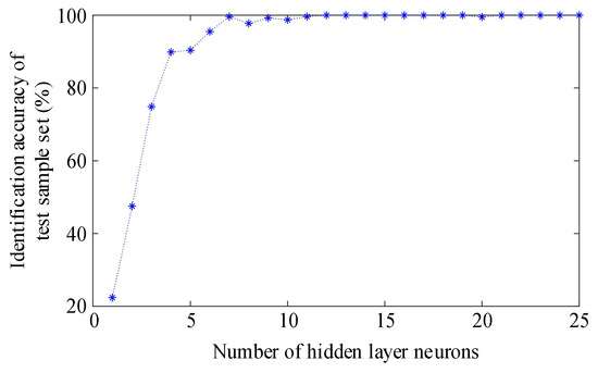
Figure 11.
The relationship between the recognition accuracy and the number of ELM hidden layer neurons.
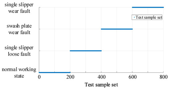
Figure 12.
The identification results of the ELM.
Under the same conditions, the BP neural network (12 input neurons, 15 hidden layer neurons, and four output layer neurons) and support vector machine (SVM) were applied to study the training samples, and the test samples were identified to obtain the identification results, as shown in Table 2.
Table 2.
Comparison of fault diagnosis results.
According to Table 2, all three fault diagnosis methods satisfactorily completed the fault diagnosis task, and, among them, the identification accuracy of ELM was the highest. Table 3 shows a comparison of the training and test times of the three methods. The training time represents the time that is required by the model to train 4000 samples, and the test time represents the time that is required by the model to identify 800 samples. It can be seen that there were big differences in the training and test times of the three fault diagnosis methods. In the training process, the BP neural network took the longest (0.75 s) and the ELM took the shortest (0.015 s). In the test process, the BP neural network took the longest (0.049 s). At the same time, SVM and ELM took the shortest (0.002 s). A large number of samples cannot be collected and the fault types diagnosed by the model are few due to the limitation of test conditions, resulting in a small model scale. With the increase of equipment complexity and fault types, the scale of fault diagnosis model will be multiplied, and the model’s ability to quickly train and process large amounts of data becomes very important. The equipment condition monitoring model needs to continuously learn and optimize the diagnostic model in the process of equipment operation, so the rapid training and fast reasoning ability of the model are particularly important. ELM will have more obvious advantages with regard to big data training and reasoning. On the whole, ELM is more efficient and suitable for online learning and fault diagnosis.
Table 3.
Comparison of training and testing times of the three fault diagnosis methods.
6. Conclusions
In this paper, the acoustic signal of an axial piston pump was collected by using a non-contact sound sensor, and the fault diagnosis method combining MFCC and ELM was adopted to realize the diagnosis and identification of the normal working state, single slipper wear fault, single slipper loose fault, and swash plate wear fault of the axial piston pump. The following conclusions were drawn:
- (1)
- In this paper, we verified that the sound sensor can be used to collect the sound signal of the axial piston pump. The characteristic information reflecting the working states of axial piston pump can be extracted through an effective data processing method. When the MFCC voice print feature extraction method was applied to the fault feature extraction of acoustic signals of the axial plunger pump, the cepstrum coefficients in MFCC were more obvious to the fault feature of the axial plunger pump, while the cepstrum coefficients in ΔMFCC were less sensitive to faults.
- (2)
- As a new learning method, ELM has obvious advantages over the traditional BP neural network and SVM in terms of training time, and it has the same test time as SVM. Therefore, the fault diagnosis method that combines MFCC and ELM has more advantages in terms of rapidity.
- (3)
- The extreme learning machine was shown to have more advantages than the BP and SVM methods by comparing the recognition accuracy and time of the three fault diagnosis methods. At the same time, the effectiveness and superiority of the fault diagnosis method of the axial piston pump based on the combination of voice print feature and ELM were fully verified.
Author Contributions
Formal analysis, Z.L.; Funding acquisition, W.J.; Investigation, Y.Z.; Methodology, J.L.; Project administration, W.J.; Resources, P.Z.; Software, Z.L.; Validation, Y.Z. and P.Z.; Writing—original draft, Z.L. and J.L.; Writing—review & editing, W.J.
Funding
This work is supported by National Natural Science Foundation of China (Grant No. 51875498, 51475405, 51805214), Key Project of Natural Science Foundation of Hebei Province, China (Grant No. E2018203339), and China Postdoctoral Science Foundation (Grant No. 2019M651722). The support is gratefully acknowledged. The authors would also like to thank the reviewers for their valuable suggestions and comments.
Conflicts of Interest
The authors declare no conflict of interest.
References
- Zhu, Y.; Qian, P.; Tang, S.; Jiang, W.L.; Li, W.; Zhao, J. Amplitude-frequency characteristics analysis for vertical vibration of hydraulic AGC system under nonlinear action. AIP Adv. 2019, 9, 035019. [Google Scholar] [CrossRef]
- Chen, B.; Wang, Z.L.; Qiu, L.H. Main developmental trend of aircraft hydraulic systems. Acta Aeronautica et Astronautica Sinica 1998, 19, 2–7. [Google Scholar]
- Zhu, Y.; Tang, S.; Wang, C.; Jiang, W.L.; Yuan, X.; Lei, Y.F. Bifurcation characteristic research on the load vertical vibration of a hydraulic automatic gauge control system. Processes 2019, 7, 718. [Google Scholar] [CrossRef]
- Niu, H.F.; Jiang, W.L. Application of hybrid approach based on immune algorithm and support vector machine for fault diagnosis of hydraulic pump. China Mech. Eng. 2008, 14, 1736–1743. [Google Scholar]
- Jiang, W.L.; Zhang, S.Q.; Wang, Y.Q. Wavelet transform method for fault diagnosis of hydraulic pump. Chin. J. Mech. Eng. 2001, 37, 34–37. [Google Scholar] [CrossRef]
- Liu, X.X.; Tan, Y.F. Research on Key Technology of Knowledge-Based Intelligent Fault Diagnosis of Hydraulic System. Appl. Mech. Mater. 2012, 241–244, 313–316. [Google Scholar] [CrossRef]
- Hao, Y.X.; Liu, Y.Y.; Zhou, J.J.; Zhou, Y.; Zheng, S.J.; Lei, C. Fault diagnosis on hydraulic driving system of shield cutterhead based on Variable-Weighted-Principal-Component-Analysis (VW-PCA). Tunn. Constr. 2018, 38, 118–123. [Google Scholar]
- Zhu, Y.; Tang, S.; Wang, C.; Jiang, W.L.; Zhao, J.; Li, G. Absolute stability condition derivation for position closed-loop system in hydraulic automatic gauge control. Processes 2019, 7, 766. [Google Scholar] [CrossRef]
- Wang, S.P.; Wang, Z.L. Fault diagnosis of hydraulic pump based on artificial neural network. J. Beijing Univ. Aeronaut. Astronaut. 1997, 6, 714–718. [Google Scholar]
- Jiang, W.L.; Chen, D.N.; Yao, C.Y. Correlation dimension analytical method and its application in fault diagnosis of hydraulic pump. Chin. J. Sens. Actuators 2004, 17, 62–65. [Google Scholar]
- Wang, S.P.; Yuan, Z.K.; Yang, G.Q. Study on fault diagnosis based on wavelet for hydraulic pump. China Mech. Eng. 2004, 15, 1160–1163. [Google Scholar]
- Peng, T.; Pei, T.R. The application of neural network method in hydraulic pump fault diagnosis. Nat. Sci. J. Xiangtan Univ. 2009, 31, 148–151. [Google Scholar]
- Tang, H.B.; Wu, Y.X.; Hua, G.J.; Ma, C.X. Fault diagnosis of pump using EMD and envelope spectrum analysis. J. Vib. Shock 2012, 31, 44–48. [Google Scholar]
- Wang, C.; Chen, X.X.; Qiu, N.; Zhu, Y.; Shi, W.D. Numerical and experimental study on the pressure fluctuation, vibration, and noise of multistage pump with radial diffuser. J. Braz. Soc. Mech. Sci. Eng. 2018, 40, 481. [Google Scholar] [CrossRef]
- Zhu, Y.; Tang, S.; Quan, L.; Jiang, W.; Zhou, L. Extraction method for signal effective component based on extreme-point symmetric mode decomposition and Kullback-Leibler divergence. J. Braz. Soc. Mech. Sci. Eng. 2019, 41, 100. [Google Scholar] [CrossRef]
- Zhao, H.X.; Yang, W.S. Vehicle recognition by acoustic signals based on short-time and Mel cepstrum coefficient. Sci. Technol. Eng. 2018, 451, 202–206. [Google Scholar]
- Yin, B.C.; Wang, W.T.; Wang, L.C. Review of deep learning. J. Beijing Univ. Technol. 2015, 41, 48–59. [Google Scholar]
- Zhu, Y.; Wang, N. Application research of identifying the empty beneath the concrete pavement slab based on Mel-scale Frequency Cepstral Coefficient. J. Qinghai Univ. 2018, 36, 27–33. [Google Scholar]
- Liu, S.S.; Tan, J.P.; Yi, Z.K. A window motor abnormal noiseidentification method based on MFCC and SVM. J. Vib. Shock 2017, 36, 102–107. [Google Scholar]
- Jiang, W.L.; Wang, H.N.; Zhu, Y.; Wang, Z.W.; Dong, K.Y. Integrated VMD denoising and KFCM clustering fault identification method of rolling bearings. China Mech. Eng. 2017, 28, 1215–1226. [Google Scholar]
- Zheng, Z.; Jiang, W.L.; Wang, Z.W.; Zhu, Y.; Yang, K. Gear fault diagnosis method based on local mean decomposition and generalized morphological fractal dimensions. Mech. Mach. Theory 2015, 91, 151–167. [Google Scholar] [CrossRef]
- Tamilselvan, P.; Wang, P. Failure diagnosis using deep belief learning based health state classification. Reliab. Eng. Syst. Saf. 2013, 115, 124–135. [Google Scholar] [CrossRef]
- Gugulothu, N.; Tv, V.; Malhotra, P.; Vig, L.; Agarwal, P.; Shroff, G. Predicting remaining useful life using time series embeddings based on recurrent neural networks. In Proceedings of the 2nd ACM SIGKDD Workshop on Machine Learning for Prognostics and Health Management, Halifax, NS, Canada, 13–17 August 2017. [Google Scholar]
- Yuan, J.S.; Zhang, L.W.; Wang, Y.; Shang, H.K. Study of transformers fault diagnosis based on extreme learning machine. Electr. Meas. Instrum. 2013, 50, 21–26. [Google Scholar]
- Wang, F.H.; Wang, S.J.; Chen, S. Voiceprint recognition model of power transformers based on improved MFCC and VQ. Proc. CSEE 2017, 37, 1535–1542. [Google Scholar]
- Lü, N.N.; Su, S.J.; Zhai, C.R. Application of improved wavelet packet threshold algorithm in vibration signal denoising. J. Detect. Control 2018, 40, 119–124. [Google Scholar]
- Dong, H.; Li, M.X.; Zhang, S.Q.; Han, L.Q.; Li, J.F.; Su, X.S. Short-term power load forecasting based on kernel principal component analysis and extreme learning machine. J. Electron. Meas. Instrum. 2018, 32, 188–193. [Google Scholar]
- Shi, P.; Yuan, Y.M.; Kuang, L.; Li, G.H.; Zhang, H.Y. Water temperature prediction in pond aquaculture based on EMD-IGA-SELM neural network. Trans. Chin. Soc. Agric. Mach. 2018, 49, 319–326. [Google Scholar]
- He, Q.; Wang, H.; Jiang, G.Q.; Xie, P.; Li, J.M.; Wang, T.C. Research of Wind Turbine Main Bearing Condition Monitoring Based on Correlation PCA and ELM. Jiliang Xuebao/Acta Metrol. Sin. 2018, 39, 89–93. [Google Scholar]
- Samal, L.; Samal, D.; Sahu, B. Recognition and Classification of Multiple Power Quality Disturbances with S-Transform and Fast S-Transform Using ELM Based Classifier. In Proceedings of the 2018 2nd International Conference on Data Science and Business Analytics (ICDSBA), Changsha, China, 21–23 September 2018. [Google Scholar]
- Zhang, Q.; Song, H.; Jiang, Y.; Cheng, Y.; Sheng, G.; Jiang, X. Partial Discharge Pattern Recognition of Transformer Based on OS-ELM. Gaodianya Jishu/High Volt. Eng. 2018, 44, 1122–1130. [Google Scholar]
- Pani, A.K.; Nayak, N. Short Term Photo Voltaic Power Prediction Using R-ELM Algorithm. In Proceedings of the 2nd International Conference on Data Science and Business Analytics (ICDSBA), Changsha, China, 21–23 September 2018. [Google Scholar]
- Wang, C.; He, X.K.; Shi, W.D.; Wang, X.K.; Wang, X.L.; Qiu, N. Numerical study on pressure fluctuation of a multistage centrifugal pump based on whole flow field. AIP Adv. 2019, 9, 035118. [Google Scholar] [CrossRef]
- He, X.K.; Jiao, W.X.; Wang, C.; Cao, W.D. Influence of surface roughness on the pump performance based on computational fluid dynamics. IEEE Access 2019, 7, 105331–105341. [Google Scholar] [CrossRef]
© 2019 by the authors. Licensee MDPI, Basel, Switzerland. This article is an open access article distributed under the terms and conditions of the Creative Commons Attribution (CC BY) license (http://creativecommons.org/licenses/by/4.0/).