Article

Using Real-Time Electricity Prices to Leverage Electrical Energy Storage and Flexible Loads in a Smart Grid Environment Utilizing Machine Learning Techniques

Department of Chemical Engineering, University of Utah, Salt Lake City, UT 84112-9203, USA
*
Author to whom correspondence should be addressed.
Processes 2019, 7(12), 870; https://doi.org/10.3390/pr7120870
Submission received: 26 September 2019 / Revised: 16 November 2019 / Accepted: 19 November 2019 / Published: 21 November 2019

Abstract

:
With exposure to real-time market pricing structures, consumers would be incentivized to invest in electrical energy storage systems and smart predictive automation of their home energy systems. Smart home automation through optimizing HVAC (heating, ventilation, and air conditioning) temperature set points, along with distributed energy storage, could be utilized in the process of optimizing the operation of the electric grid. Using electricity prices as decision variables to leverage electrical energy storage and flexible loads can be a valuable tool to optimize the performance of the power grid and reduce electricity costs both on the supply and demand sides. Energy demand prediction is important for proper allocation and utilization of the available resources. Manipulating energy prices to leverage storage and flexible loads through these demand prediction models is a novel idea that needs to be studied. In this paper, different models for proactive prediction of the energy demand for an entire city using different machine learning techniques are presented and compared. The results of the machine learning techniques show that the proposed nonlinear autoregressive with exogenous inputs neural network model resulted in the most accurate predictions. These prediction models pave the way for the demand side to become an important asset for grid regulation by responding to variable price signals through battery energy storage and passive thermal energy storage using HVAC temperature set points.

1. Introduction

The rapid adoption of variable renewable energy sources (VREs) is creating a growing need for energy storage, flexible loads, and smart automation technologies for better management of a fluctuating electric grid. In deregulated markets, market mechanisms are used at a wholesale level to ensure that supply meets the demand. However, in the vast majority of markets, small- and medium-scale end users are insulated from the market and have fixed or simplified electric rate structures. While there are reasons for this simplicity, it removes any incentive for these end-users to invest in storage or smart scheduling technology. With a flat rate, for example, only total energy consumption matters, financially, to customers. Alternatively, if customers had variable, or even real-time prices, when they use energy might be as important as how much energy they use. This would create a financial incentive for them to invest in battery storage technologies and to use systems that automate their energy usage (such as with smart HVAC scheduling). This would be difficult or impossible for consumers to manage on their own. However, with optimization-based, proactive automation to charge and discharge the battery as well as manage HVAC set points, the consumer would not have to manage their energy usage actively. The combination of variable prices reflecting supply and demand on the market, widespread adoption of energy storage, and smart automation technologies have the potential to transform energy users into a valuable asset for grid management. While there are substantial regulatory hurdles for this scenario to become a reality, the purpose of this paper is to model, at the grid level, the potential impact of the confluence of these three factors and to develop energy demand prediction models would represent this system. The developed energy demand prediction models would then be used, in future studies, to optimize the operation of the grid.
Demand-side management (DSM) is an essential part of a smart grid that creates a decision platform for key stakeholders to trade energy between the consumers and providers [1]. DSM is defined as the planning and implementation of those activities designed to influence consumer use of electricity in ways that will result in changes in the utility’s load shape [2]. Different DSM techniques are being practiced throughout the world with several targets. Among these targets are the following: increasing energy efficiency by reducing demand in the long term and employing demand response programs that can influence the demand in the short term in response to variable energy price signals. The formulation and impacts of DSM models and techniques on the smart grid have been widely studied in the literature. Many researchers have proposed models to perform load shifting in smart grids with the inclusion of electric vehicles [3,4,5]. Other researchers have studied DSM for smart building automation [6,7,8,9]. In fact, studies related to DSM and its impact on the power sector cannot be just summarized in a few lines. However, various review articles have deeply discussed and surveyed these issues [10,11,12,13].
With the presence of DSM along with multi-scale renewable generation, energy demand prediction is becoming important as it helps to improve the efficiency of the smart grid network on both the distribution end and the generation stations [14,15]. Different techniques have been proposed for energy load forecasting in recent years. Computational intelligence for energy forecasting can use a single machine learning model or hybrid models. Single models include fuzzy logic sets, artificial neural networks (ANN), support vector machines (SVM), linear and nonlinear regression, clustering techniques, genetic algorithms (GA), artificial bee algorithm, artificial immune systems (AIS), and particle swarm optimization (PSO). Hybrid models include neuro-fuzzy (NF), artificial neural network and wavelet transform, optimization algorithms integrated with ANN, ANN and clustering techniques, and optimization algorithms integrated with SVM. Fallah et al. discussed the aforementioned techniques showing the advantages and disadvantages of each of them and the challenges for the future [1]. Many researchers have developed different models and optimization techniques for predicting the energy demand for various entities of the demand side of the electricity grid using machine learning mainly for minimizing the operational cost or optimizing energy usage [16,17,18,19]. Other researchers have developed energy demand prediction models, scheduling techniques, and energy management systems considering the demand side and the supply side as well for several purposes, including cost minimization and grid frequency control [20,21,22]. Dahraie et al. presented a scheduling approach to balance the supply and demand with an overall purpose of minimizing the operational cost taking into consideration the constraints related to the maximum and minimum capacities of the included energy storage devices and renewable energy resources under different demand response programs [23]. Muralitharan et al. developed an energy demand prediction model and mentioned that with the developed model it would be possible to improve the management of demand and supply, planning of power grid and prediction of future energy requirement in the smart grid, but the authors never mentioned how the developed model would do so [15]. To the best of our knowledge, no deeper investigation has been done into how energy price signals with a real-time pricing structure (RTP) would affect the energy demand required from non-renewable energy resources (e.g., thermal power plants) in a smart grid environment. Using energy price signals as a manipulated variable to leverage battery energy storage and flexible loads (i.e., air conditioning temperature set points) within residential buildings is a novel idea that needs to be addressed.
This study aims to illustrate how using price signals as decision variables would encourage homeowners to use energy storage systems and flexible loads to reduce their bills significantly. In doing that, energy demand prediction models were developed using weather forecasts, historical demand data, and energy price signals. Three different single model machine learning techniques have been used to develop the demand prediction models; linear autoregressive with exogenous inputs regression model (L-ARX regression model), nonlinear autoregressive with exogenous inputs regression model (N-ARX regression model), and nonlinear autoregressive with exogenous inputs neural network (N-ARXnet model). A smart grid model for a city of 60,000 houses is presented to illustrate the relationship between all the parameters of the grid and how making the energy price signals a decision variable would affect the control and operation of the grid. The energy demand prediction models presented in this study will be used to solve a grid-level optimization problem in another future study. The ultimate goal is to motivate homeowners to invest in ESS and to encourage policymakers to implement real-time pricing rate structures while making them available to homeowners.
The remainder of this manuscript is organized as follows. Section 2 presents the smart grid model and its components in general. Section 3 presents the model formulation, including the smart houses, solar power plant, conventional natural gas thermal power plant, and frequency control. Problems related to the electricity grid and potential solutions using energy prices are discussed in Section 4. A clear illustration of the novelty of this work is presented in Section 4. A description of the machine learning techniques used is presented in Section 5. The results and discussion are presented in Section 6. Finally, the conclusion and future work are summarized in Section 7.

2. System Description

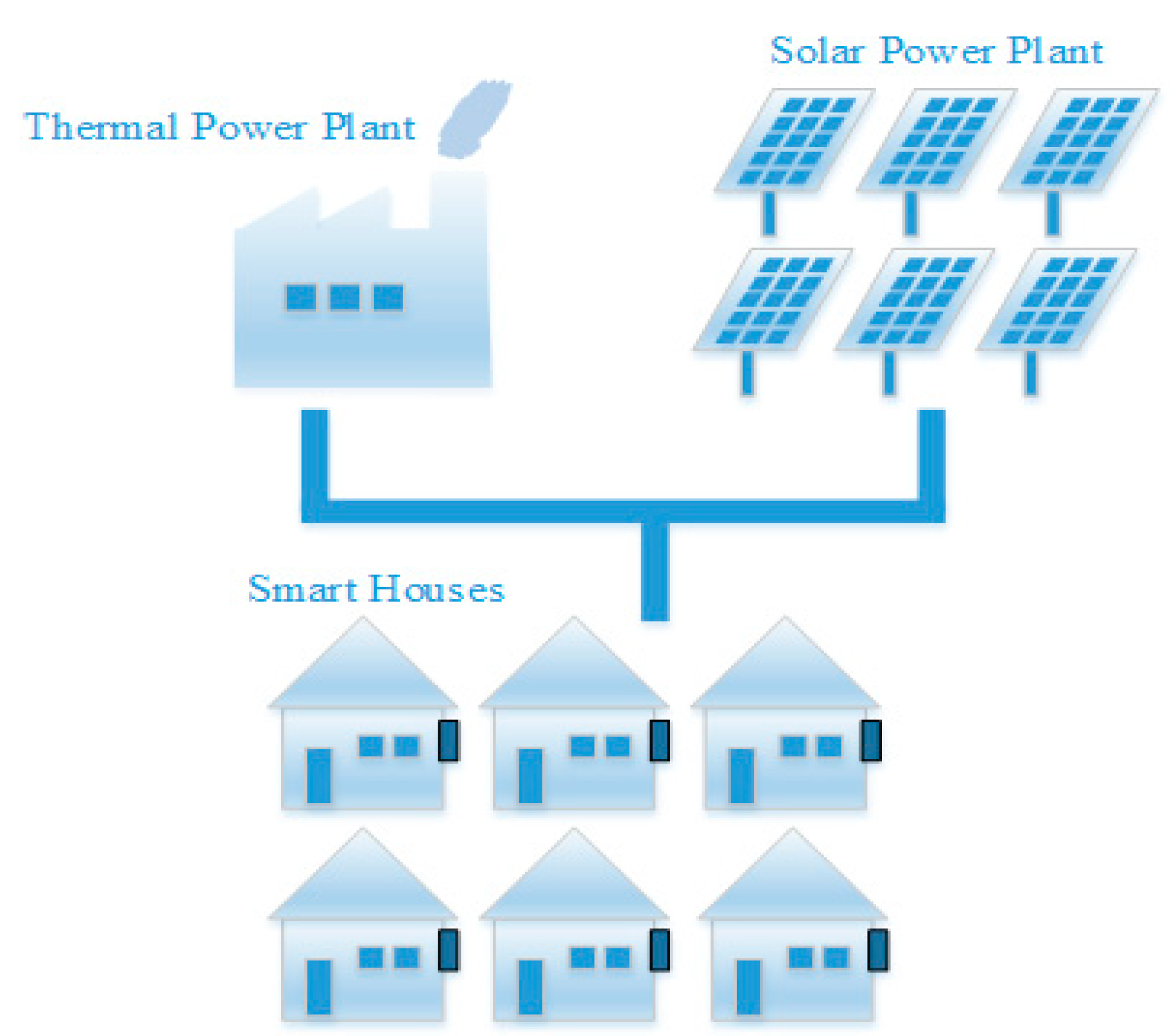
The smart grid system used in this study is composed of a city of 60,000 houses, a solar power plant, and a thermal power plant.
Figure 1 shows a simple schematic of the system. The first element of the grid is the smart houses representing the power demand for a city of 60,000 houses. The houses are referred to as smart houses because of the smart automation of the HVAC system implemented within each house, in addition to the use of battery energy storage.
The second element of the grid is a conventional natural gas thermal power plant. While the thermal power plant is the primary energy source in this study, it is flexible and dispatchable, so it is used as a manipulated variable to regulate the frequency of the grid at 60 Hz. Figure 2 illustrates the operation of the grid. The energy demand from the city, together with the generated power from the thermal and solar power plants are used to calculate the frequency of the grid. Each house in the city has a proactive energy management system, where it charges or discharges the battery and regulates the HVAC temperature setpoint based on the price signals and the weather forecast. The calculated frequency is then sent to a PI controller, which has a set point of 60 Hz. The PI controller determines the required generation from the thermal power plant that would keep the frequency of the grid at 60 Hz using a very tight control scheme.
The third element of the grid is a solar power plant. The solar power plant is a secondary power supply that provides energy as available from the sun while relying on the thermal power plant to regulate the frequency and to ensure that supply meets demand at all times. In this model, the size of the solar plant can be changed to determine how much solar energy the aforementioned storage and automation techniques can accommodate.
The model formulation of the system, including the houses energy management systems, solar power plant, thermal power plant, and the energy demand models is discussed in Section 3.

3. Model Formulation

3.1. Smart Houses

Different models in the literature have been used for home modeling applications [24,25,26]. In this study, the model developed by Sheha and Powell was used to simulate the smart houses [27]. In this model, the rate of change of the indoor temperature within each house is described by the following equation:
A d T d t = B ( T a m b T h o u s e ) Q + C
Typical meteorological year (TMY3) weather files for Salt Lake City, Utah, were used to simulate the ambient temperature. This is only for research purposes, but for an actual system, accurate weather predictions should be used instead of TMY3 data. The term “A” accounts for the total thermal masses of each house, while the term “B” accounts for the overall heat transfer coefficient and surface area through the boundaries of each house. The term “C” is a constant term accounting for any neglected sources that might affect the indoor temperature (e.g., ground temperature, direct normal irradiance, etc.). The term “B” for each house was determined using the relevant data extracted from BEopt (building energy optimization) software (National Renewable Energy Laboratory, Golden, CO, USA), while the term “C” was a fitting parameter to make the results of the model close enough to the results of BEopt. “Q” represents the cooling energy within each house. The effect of ground temperature, direct normal irradiance, relative humidity, etc., was found to be negligible, but was still taken into account through the term “C.”. More details about this simplification can be found in the study done by Sheha and Powell [27].
The main feature of the smart houses used in this study is cost optimization. The model developed by Sheha et al. was used to perform the cost optimization within each house [28]. Cost optimization is formulated as a linear programming problem with multiple decision variables. Those decision variables are the hourly temperature set points of the air conditioner over 24 h, the hourly energy input to the battery over 24 h, the hourly energy output from the battery over 24 h, and the hourly state of charge of the battery for the same period. Note that the prediction horizon is 24 h, not one hour, but only the results for the first hour get implemented and then the optimization problem gets solved again for the next 24 h, and so on. This is because of the variability in the weather forecast that gets updated continuously and to avoid any system/model mismatch. For example, the house model might not be able to reach the targeted set point obtained from the optimization problem within the specified hour, which changes the initial condition for the next hour. The objective function of the problem is described in Equation (2).
min i = 1 24 R i × ( Q i + P C i P D C i )
where R is the electricity price in $/kWh, Q is the cooling electricity consumption in kWh, P C is the charging energy of the battery, and P D C is the discharging energy of the battery.
The optimization is subject to two equality constraints every hour, which are the discretized form of Equation (1) and the discretized form of the following battery function:
d ( S O C ) d t = η C P C P D C η D C
where d ( S O C ) d t is the rate of change of the state of charge of the battery with time in kWh per unit time. η C and η D C are the charging and discharging efficiencies of the battery, respectively. Note that, there is no such case where the battery can both charge and discharge at the same time. Thus no constraints are needed to ensure this.
Also, each decision variable is subject to a lower and upper bound. Table 1 summarizes all the optimization formulation equations together. The operating range for the temperature setpoint expands during the unoccupied period of each house. Standard home battery capacities were used as per the Tesla Powerwall, which has two different designs; 6.4 kWh and 13.5 kWh maximum capacities [29]. Note that, for this study, it was assumed that the battery SOC could reach a value of zero. This is just a theoretical assumption used in this study, but a real battery shall have a minimum SOC, which is not zero.
The electricity pricing structure used is real-time pricing with prices ranging from −0.1 $/kWh to 0.23 $/kWh, with the average daily energy price being 0.11 $/kWh, which is the average energy price in Utah [30]. A negative energy price is a possible scenario that might happen when the grid becomes a net producing grid (i.e., the energy demand is less than the energy supply). At this time, an incentive to let people use the grid energy is to impose a negative energy price (i.e., pay money to the consumers who would use energy from the grid at this time to balance supply and demand). Eleven different real-time pricing profiles within the same range of prices were used, where one of them is used for training the machine learning methods, and the other ten profiles are used for validating the resulting models. Figure 3 illustrates the 11 real-time pricing profiles used throughout four days in August. Notice that for each profile, the price is varied every four hours to allow enough time for the model to catch the effect of the changes happening within the system. The top left price profile in (highlighted in red color) is the one used for the training and validation phases, while the other ten profiles are used for the testing phase. The system was solved dynamically in a real-time optimization form (D-RTO) using Matlab/Simulink.
In this paper, only the cooling systems are studied, nothing related to home heating systems is studied because the houses are assumed to be gas heated. The cooling system of each house is formulated as a feedback PI controller, where the controller takes the indoor temperature and the setpoint temperature of each house and then adjusts the required cooling energy based on how far the indoor temperature is from the temperature set point. This description is illustrated in Figure 4.

3.2. Solar Power Plant

A solar plant model with 100,000 solar panels and a standard panel size of 39 × 78 is used in this study. The following equation determines the power produced per panel:
P = S × A × η p a n e l
where P is the produced power, S is the absorbed solar radiation, A is the panel area, and η p a n e l is panel efficiency. A panel efficiency of 22% is used in this study. The effect of panel temperature on its efficiency is neglected and is outside the scope of this study.
The absorbed solar radiation is obtained from [31]:
S = ( τ α ) n M [ G B R B K θ , B + G D K θ , D ( 1 + cos β 2 ) + G ρ G K θ , G ( 1 cos β 2 ) ]
The definitions of the different terms in Equation (5) and their calculations are listed in Appendix A.

3.3. Natural Gas Thermal Power Plant

The energy produced from the thermal power plant is employed as a manipulated variable to control the frequency of the grid at 60 Hz. The rate of change of the frequency of the grid is calculated from the following differential equation:
d f d t = P t h e r m a l + P s o l a r P d e m a n d τ
where d f d t is the rate of change of the grid frequency per unit time, P t h e r m a l is the power produced from the thermal power plant, P s o l a r is the power produced from the solar power plant, P d e m a n d is the power demand from the city of 60,000 houses, and “ τ ” is a constant representing the inertia of the grid itself.
A PI controller to regulate the frequency of the grid was used with a set point of 60 Hz and with the power produced from the thermal power plant being the manipulated variable. The PI controller takes in the frequency reading at every time step and adjusts the required power from the thermal power plant accordingly based on how far the frequency is from the set point of 60 Hz. The control has to be tight and keep the frequency at almost 60 Hz at all times to avoid any complications within the grid, such as power shortage or overloading. Figure 5a illustrates the frequency profile over ten days during May, and Figure 5b illustrates the supply and demand profiles for the same period. Notice the tight control over the frequency in Figure 5a.

4. Scenarios with the Operation of the Grid

4.1. Scenarios Description

Higher levels of solar penetration are foreseen in the future of the grid. When using the developed grid model and different levels of solar penetration, some challenges start to appear. Figure 6 illustrates the net energy demand (required production from the thermal power plant) at different levels of solar penetration with no consideration of the pricing structure and no smart home automation. The net demand drops down as solar production increases. Researchers refer to this drop in demand as the “duck curve” [32]. Potential problems that could arise from this duck curve are overgeneration during the periods of solar irradiance availability and extreme ramping requirements at the periods of falling solar irradiance. In Figure 6, net demand 5 goes below zero from 12:30 PM until 2 PM. This negative value means that the overgeneration problem is happening at this period. Also, net demand 5 moves from a value of almost zero to a value of over 100 MWh in roughly four hours. Depending on the thermal power plant configuration, this big change might be achievable but puts increased strain on the grid. Each power plant has its capabilities regarding starting up the plant and reaching maximum capacity in a certain amount of time. High levels of solar penetration might create this ramping problem, especially during the sunset period. Another potential problem, in general, is that the thermal power plant’s maximum production capacity might not be enough to handle the system at night. These problems introduce the need for smart home automation along with a variable energy pricing structure to help in optimizing grid-level energy demand.

4.2. Using Prices as a Grid Regulatory Mechanism

Figure 7 presents the same net demand 5 from Figure 6 vs. a case that has the same level of solar penetration and proactive energy management systems within the houses by utilizing variable/real-time price signals. It can be observed that using real-time pricing increases the energy demand when the energy price is lower (batteries charging and lower indoor temperature set points) and decreases the energy demand when the energy price is higher (batteries discharging and higher temperature setpoints). Note that, in the period from 12 AM till 6 AM, the ambient temperature is low (no air conditioning is needed), the residents are not using a lot of electricity (mainly they are using the fridge and maybe some lighting), the electricity prices are high (no incentive to charge the battery), and the battery is empty at its initial condition so there is no energy to be discharged from the battery. Thus, there is no incentive for load shifting during this period. The real-time pricing profile presented in Figure 7 was found using the manual trial and error over the system. Different hypothetical real-time pricing profiles have been tried until one of them managed to flatten the net energy demand curve significantly. These results demonstrate that, by manipulating prices only, consumers with storage and proactive automation could significantly alter the net demand profile. The optimized energy demand reduces the ramping requirements of the power plant, decreases the maximum required capacity, and has no overgeneration. This suggested criterion is novel and has never been studied before in the literature. While Figure 7 demonstrates the impact that prices can have on net demand, there remains a much larger problem of developing predictive models to determine, quantitatively, the impact that the prices will have on the net demand, which is the focus of this work. Future work will seek to optimize these pricing profiles, systematically instead of manually, to minimize the extreme ramping by the thermal power plant and to accommodate as much solar power as possible, while maintaining stable grid frequencies.
A numeric relation between electricity prices and the energy demand needs to be developed to solve this optimization problem. In other words, energy demand prediction models need to be developed using energy prices as inputs. These prediction models would use energy price and environmental conditions as inputs and give the energy demand of the city as an output. These models would then be incorporated into the optimization problem with the energy prices being the decision variables. Different values for the energy prices would affect the local optimization at each house that would utilize the variable prices to optimize air conditioning systems (passive thermal energy storage) and battery energy consumption (electrical energy storage), thus affecting the total energy demand of the city by leveraging energy storage (novelty of this work).
This paper focuses on developing energy demand prediction models and comparing them based on their performance vs. actual model data. A future study will focus on the grid-level optimization problem utilizing the developed models in this current study. The big picture is to explore the impact that variable electricity prices in the residential sector, combined with energy storage and proactive energy management systems, can have on the grid.
Because the grid is complex and the economic relationships between supply and demand cannot be easily modeled with engineering principles, data-driven models are required. Furthermore, because the problem to be solved is fundamentally one of energy storage, these models must be dynamic, with time interdependencies caused by the battery storage and the passive thermal storage in the homes. For these reasons, machine learning models incorporating dynamics are used.

5. Machine Learning Techniques

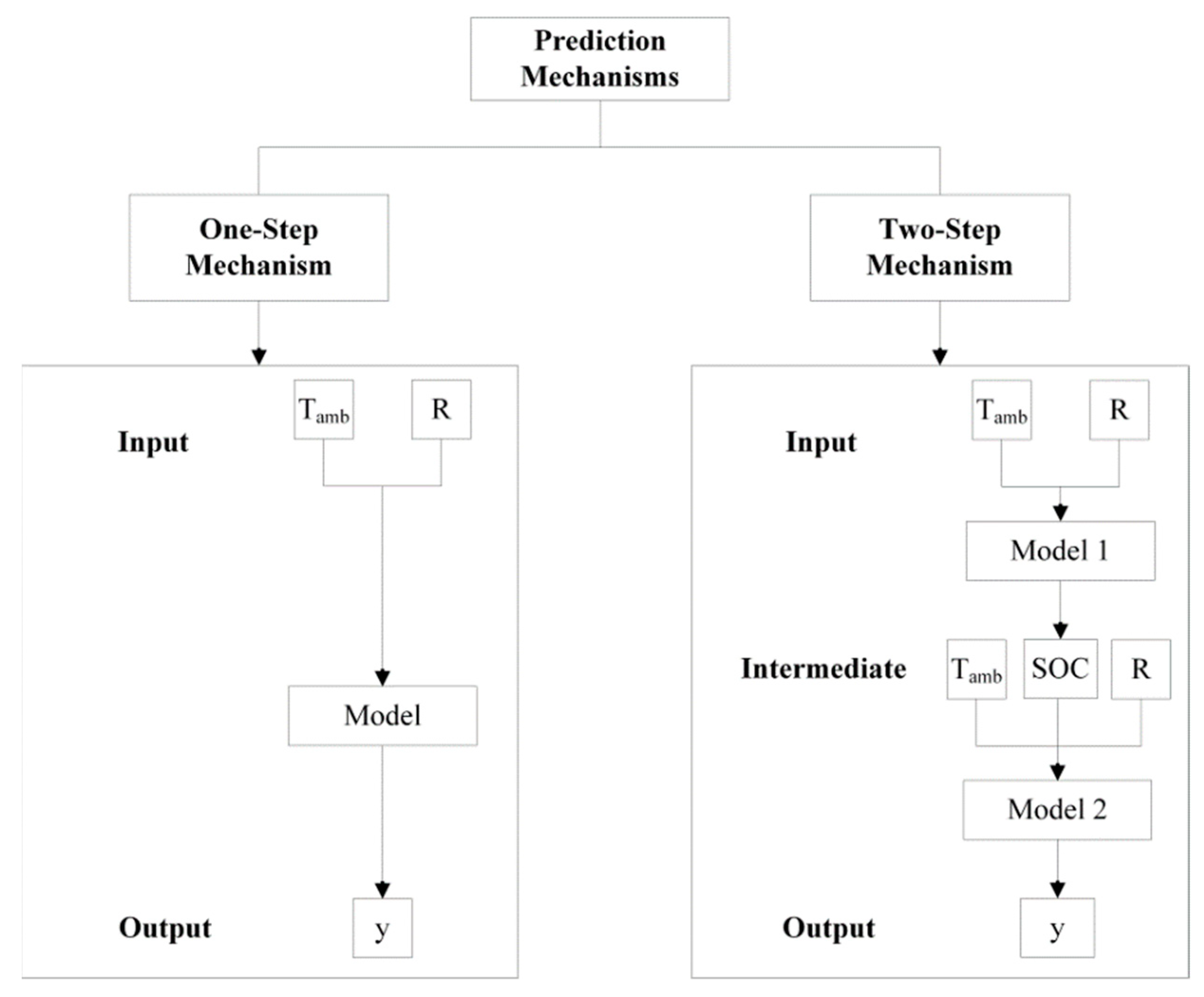
For this study, three different techniques were used with two different prediction mechanisms: a one-step mechanism and a two-step mechanism. Figure 8 illustrates the three machine learning techniques, while Figure 9 illustrates the two prediction mechanisms. As presented in Figure 8, the three methods are linear autoregressive with exogenous inputs regression model (L-ARX Model), non-linear autoregressive with exogenous inputs regression model (N-ARX Model), and non-linear autoregressive with exogenous inputs neural network model (N-ARXnet Model). L-ARX and N-ARX regression techniques were used because they represent the simplest forms of machine learning for linear systems and nonlinear systems, respectively. If the system can be well represented with one of these simple forms, then there will not be any need for using a more complex technique that would make the problem computationally expensive. The N-ARX neural network technique was used because it showed good potential in solving different complex systems in the literature in the same field [33,34,35]. Autoregressive models were used because of the temporal nature of demand. Actually, a standard feedforward neural network was tested first but gave poor results and thus was neglected and substituted by an autoregressive neural network with exogenous inputs. As discussed earlier in the introduction, many different machine learning techniques can be used, but for this study, only the three aforementioned techniques were used. Using a wider range of techniques is a good idea and could be the focus of future studies, but this study is trying more to convey the idea of using variable price signals to leverage storage and flexible loads than to compare a lot of machine learning techniques.
For each method, two mechanisms are applied, as illustrated in Figure 9. For the one-step mechanism, only one model is formulated with two inputs: ambient temperature and price signals. The model, as well, considers old demand values as inputs. For the two-step mechanism, two models are used: one to predict the total battery SOC for the city, then the second model is used to predict the demand by taking the predicted values for the SOC as inputs in addition to the ambient temperature and the price signals.
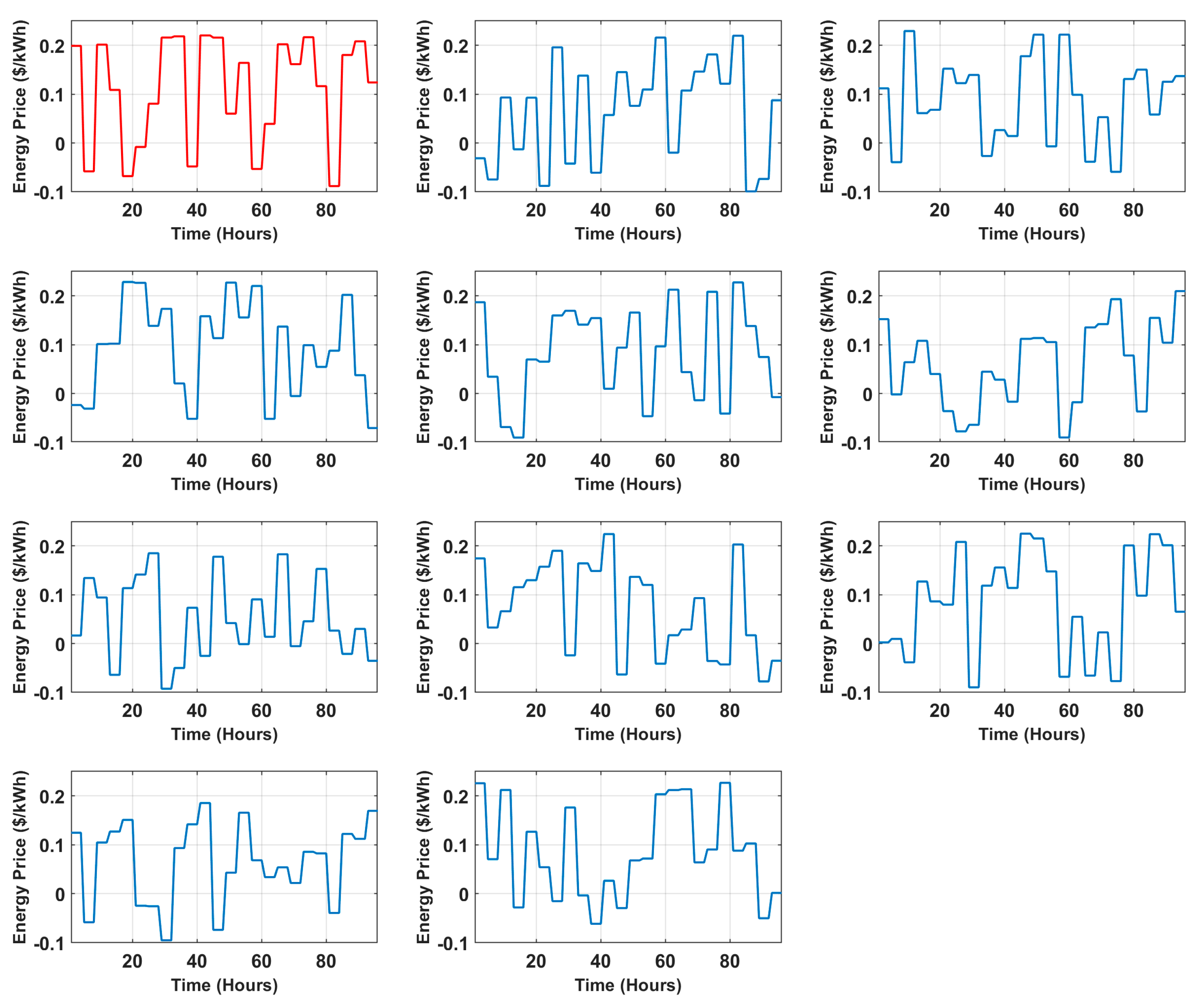
In developing the models, the pricing profile shown in red color in Figure 3, along with the corresponding energy demand was used for the training and validation phases, while the rest of the pricing profiles of Figure 3 were used for the testing phase. The dataset used for training and validation was divided into two datasets; one for training (80% of the data points) and one for validation (20% of the data points). The number of old demand values (number of lags) used as inputs was tuned in the validation phase until a value of three hours of previous energy demand data (12 data points because of the 15 min time interval) was chosen as an optimal value. More hours of lag did not result in any significant improvement in the results and would only increase the computational time, while fewer hours did not give good enough results. The developed models are described as follows.

5.1. Linear ARX Regression Models

Linear regression is a method of identifying the relationship between correlated inputs and outputs of a certain system by only including linear terms in the relation between them. ARX model (autoregressive with exogenous inputs) means that the model uses previous output values as inputs to the system with additional new inputs as well. The L-ARX regression models used in this study were developed using new codes written by the authors in Matlab. A “base case” L-ARX regression model that does not include the electricity prices in the inputs was considered and has the following form:
y t = a + i = 1 108 b i T a m b i + i = i 8 c i y t i .  
By including electricity prices in the inputs, the following one-step model was developed for predicting the energy demand using L-ARX regression:
y t = a + i = 1 108 b i T a m b i + i = 1 108 c i R i + i = i 8 d i y t i
where y t is the energy demand of the city at time “ t ” in MWh and a , b i , c i , and d i are the model coefficients. Note that the time step is 15 min, which means that in every hour there are four points or four-time steps. The 108 points in the second and third term are the time steps for 27 h (24 h in the future and three hours in the past) and calculated like this: 27 × 4 = 108 . For the 4th term, two hours of past demand values are used (eight-time steps in the past).
Equations (9) and (10) represent the two-step L-ARX regression model as follows:
S O C t = a + i = 1 108 b i T a m b i + i = 1 108 c i R i + i = i 8 d i S O C t i
y t = a + i = 1 108 b i T a m b i + i = 1 108 c i R i + i = 1 8 d i y t i + e S O C t
where S O C t is the total state of charge of the city at time “ t ” in MWh. Notice that the values of the model coefficients are different for each equation.

5.2. Nonlinear ARX Regression Models

Nonlinear regression is a method used to identify the relation between correlated inputs and outputs of a system by including all different combinations between the terms either linear or nonlinear. In this study, multiple possible N-ARX expressions have been tested starting from basic quadratic functions up to the complicated expressions shown in Equations (11)–(13). These expressions were chosen because they gave the best regression results among all the tested models. The N-ARX regression models used in this study were developed using new codes written by the authors in Matlab. The following expression represents the one-step model that was developed for predicting the energy demand using N-ARX regression:
y t = a + i = 1 108 b i T a m b i + i = 1 108 c i R i + i = 1 108 d i R i 2 + e y t 1 + i = 1 108 y t 1 ( f i R i + g i R i 3 + h i R i 4 + j i R i 5 ) + k y t 2 + i = 1 108 y t 2 l i R i + m y t 3 + i = 1 108 y t 3 ( n i R i + q i R i 3 ) + s y t 4 + i = 1 108 y t 4 ( u i R i + v i R i 3 ) + i = 5 8 w i y t i
Equations (12) and (13) represent the two-step N-ARX regression model as follows:
S O C t = a + i = 1 108 b i T a m b i + i = 1 108 c i R i + i = 1 108 d i R i 2 + e S O C t 1 + i = 1 108 f i S O C t 1 R i + g S O C t 2        + h S O C t 3 + i = 1 108 S O C t 3 ( j i R i 2 + k i R i 3 + l i R i 4 ) + i = 4 8 m i S O C t i
y t = a + i = 1 108 b i T a m b i + i = 1 108 c i R i + i = 1 108 d i R i 2 + i = 1 108 e i R i T a m b i + i = 1 108 f i R i y t 1 + i = 1 4 g i y t i + h S O C t
The number of terms in the two-step N-ARX regression model is less than the number of terms in the one-step model. This is because, during the tuning of the two-step model, it was observed that using more terms results in overfitting that reduces the accuracy of the results. Again, note that all the model coefficients in Equations (7)–(13) are all different.
Notice that, if the cost terms were removed from the one-step methods presented in Equations (8) and (11), they would have the same form, which is exactly the “base case model” presented in Equation (7). The only difference would be the model coefficients.

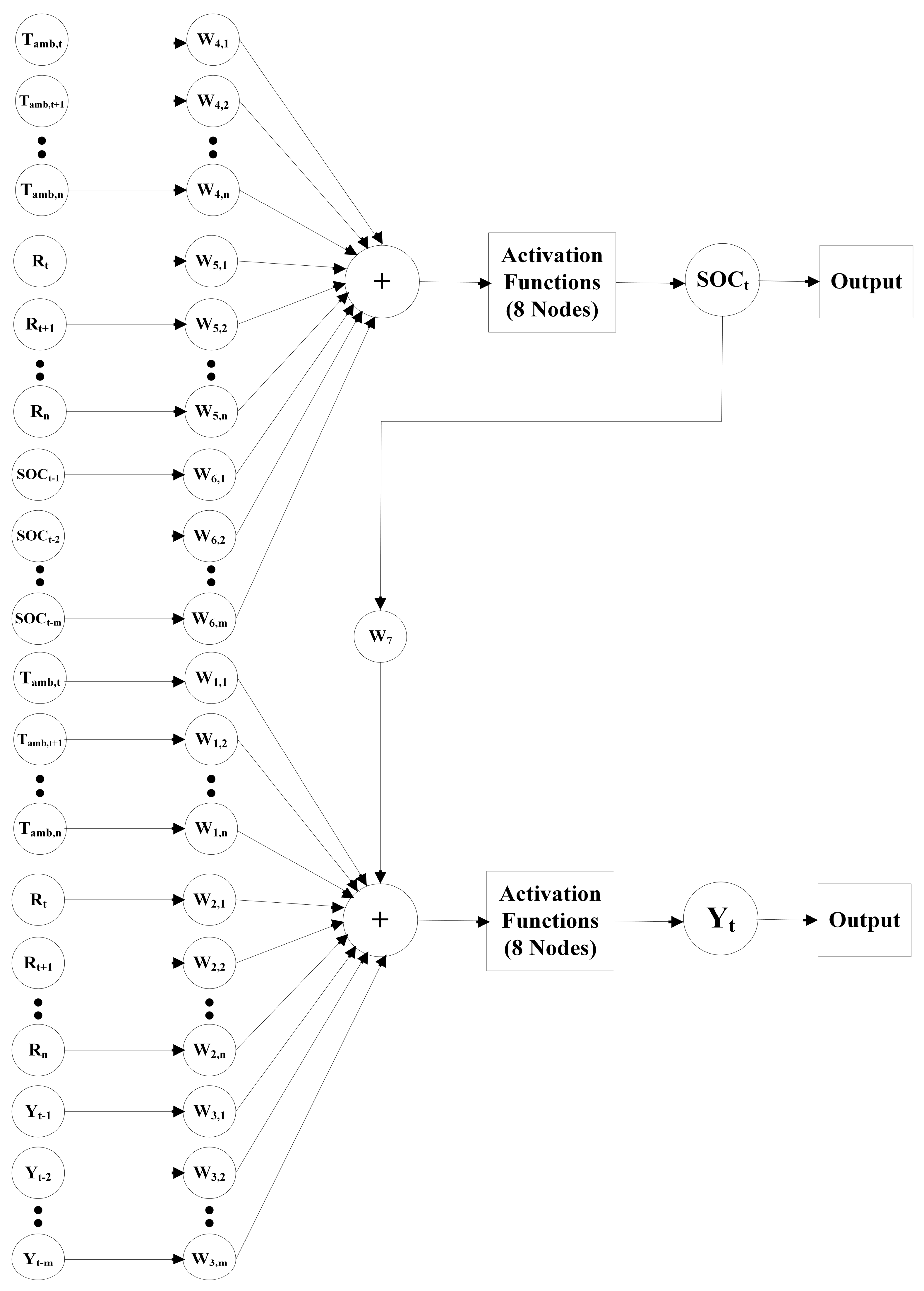
5.3. Nonlinear ARX Neural Network Model (N-ARXnet)

N-ARXnet is an artificial neural network where the outputs are fed back and used as inputs that form a cycle, with new inputs always added at every time step (i.e., N-ARXnet has two different time series, one for the feedback inputs and one for the new inputs). In this study, a three-layer perceptron is used. The three layers are input, hidden, and output layers. The N-ARX neural network models used in this study were developed using “narxnet” function available within Matlab. A “base case” N-ARXnet is considered in this study, which does not have electricity prices as inputs. Figure 10 illustrates the structure of the N-ARXnet used as a base case, while Figure 11 illustrates the structure of the N-ARXnet used for the one-step prediction mechanism. For the one-step mechanism, the new inputs at every time step are the 24-h ahead ambient temperature values and 24-h ahead energy prices. Two different time series are used with a three-hour difference. This means that the demand values for the previous three hours are fed back as inputs for each time step and three hours of previous values of the new inputs (ambient temperature and energy prices) are used as well. W i , j is the weight for each input and Y is the output. The network was tuned with different numbers of nodes until an optimal value of eight nodes was chosen because a bigger number of nodes did not show any significant improvement in the results and would result in overfitting problems. Remember that the time step is 15 min, which means that 12 past values of the energy demand are fed back to the inputs. The same criteria used for the one-step mechanism were also used for the two-step mechanism with the SOC included in between as shown in Figure 12. First, a network was tuned to predict the SOC. Then the results from this SOC network were used as input in the tuning of the second network to predict the energy demand.
The results for the training, validation, and testing of all three machine learning techniques are presented and discussed in Section 6 (Results and Discussion).

6. Results and Discussion

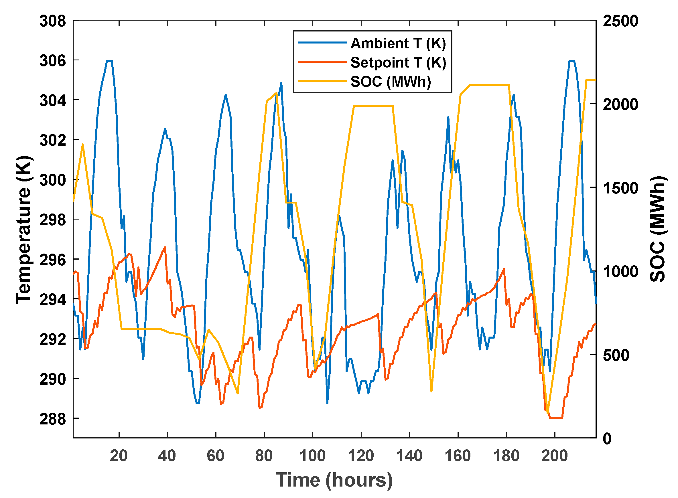
To illustrate the complexity of the input dynamic Simulink model, Figure 13 presents a 10-day profile of the ambient temperature, the temperature setpoint of one of the houses, and the total state of charge (SOC) of all houses. Note that, these are not the only variables of the system; the data for each house includes, as well, lighting, energy consumption from kitchen appliances (e.g., refrigerator, stove, microwave, etc.) and plug loads (e.g., computers, printers, fans, etc.). Although lighting, kitchen appliances, and plug loads have minor effects compared to HVAC and batteries, they are still taken into consideration. In addition to these data, there is also the variable pricing profiles, which has been illustrated in Figure 3. From Figure 13, it can be noticed that there is no specific trend for any of the plots, except that the ambient temperature, of course, goes to lower values at night and higher values during daylight. However, the ambient temperature might stay at relatively lower values for a whole day (as in the period from 100 to 120 h on the plot). Putting all of these together, while considering 60,000 houses, gives a sense of the extremely complex system under study. Building a model with machine learning to represent this complex system with limited input information (just ambient temperature and price signals) was not an easy task.
The three methods used were trained and validated for the summer period (May through September) using ambient temperature obtained from TMY3 weather data for Salt Lake City, Utah and random energy price profiles as inputs for the system and the energy demand resulting from the Matlab/Simulink smart grid model as the system output. As mentioned earlier, the houses are assumed to be gas heated. In this study, the winter months which involve most or all the space heating were not accounted for in the developed models. Different models would need to be built to account for the space heating by natural gas, not electricity and this is out of the scope of this study. The coefficient of determination, root mean squared error, and normalized root mean squared error were used to compare and evaluate the performance of each resulted model.

Training, Validation, and Testing

The results of the training and validation of each model are illustrated in the parity plots shown in Figure 14. The main observation that can be drawn from the parity plots is that there are some residuals when the value of the demand is close to zero, and this is visible especially in the parity plots of the L-ARX regression models (Figure 14a–c). Generally, this makes sense because it is harder to correlate the data when their values are closer to zero. Also, in Figure 14a,f (base case models), it can be noticed that the points are more dispersed than all the other parity plots. Notice that, for example in Figure 14a (base case L-ARX model parity plot), the range of the error is very big to the level that some points have actual demand values above 600 MWh while the corresponding model values are negative. This means that electricity prices have significant effect on the parity plots.
Another important observation is that the data are more dispersed in Figure 14b–e than in Figure 14g,h. This means that the N-ARXnet models have a better performance than the L-ARX and N-ARX regression models. However, only observing the parity plots is not enough for quantifying the performance of each model. Therefore, the coefficient of determination, root mean squared error, and normalized root mean squared error were used to quantify and compare the performance of all the developed models. Table 2 presents the results of these metrics for each model with the training and validation dataset vs. the results with testing datasets.
Different energy price profiles (Figure 3) from 10 different datasets were used to test the developed models. Variations in the ambient temperature were considered minor and were not taken into consideration. However, separate studies should be performed to evaluate the effect of the uncertainty resulting from TMY3 weather data. 
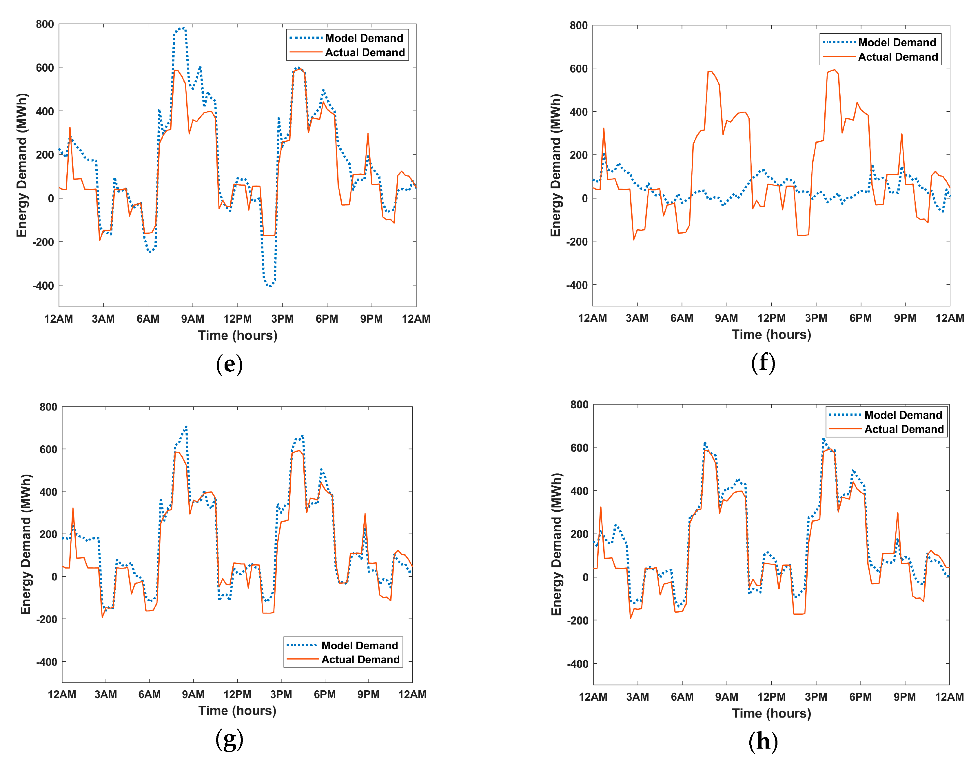
Figure 15 presents the energy demand calculated using the training and validation dataset vs. the energy demand calculated using one of the testing datasets for all models. The most obvious observations are in Figure 15a,f (base case models that do not account for electricity prices) which show that the models completely failed in matching the actual data. This proves that electricity prices are crucial parameters and have to be considered in the models.
From Figure 15b,c, it can be noted that the L-ARX regression models have poor performance when different input dataset is used. Notice that the model failed to predict the maximum demand values at around 8 AM and 4 PM. The N-ARX regression models have a better performance than the L-ARX regression ones, and the N-ARXnet models have slightly better performance than the N-ARX regression models.
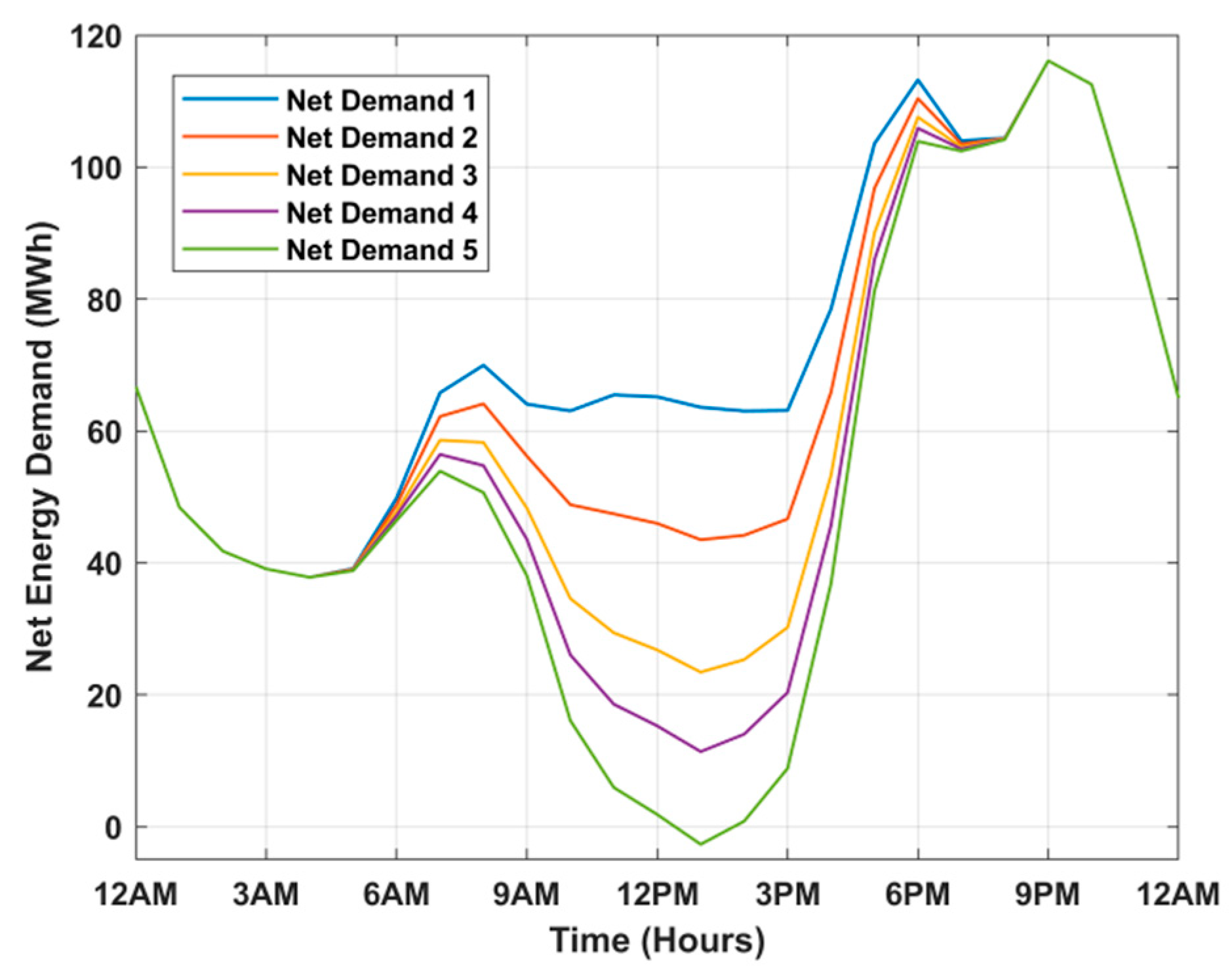
On the other hand, it can be noted from 
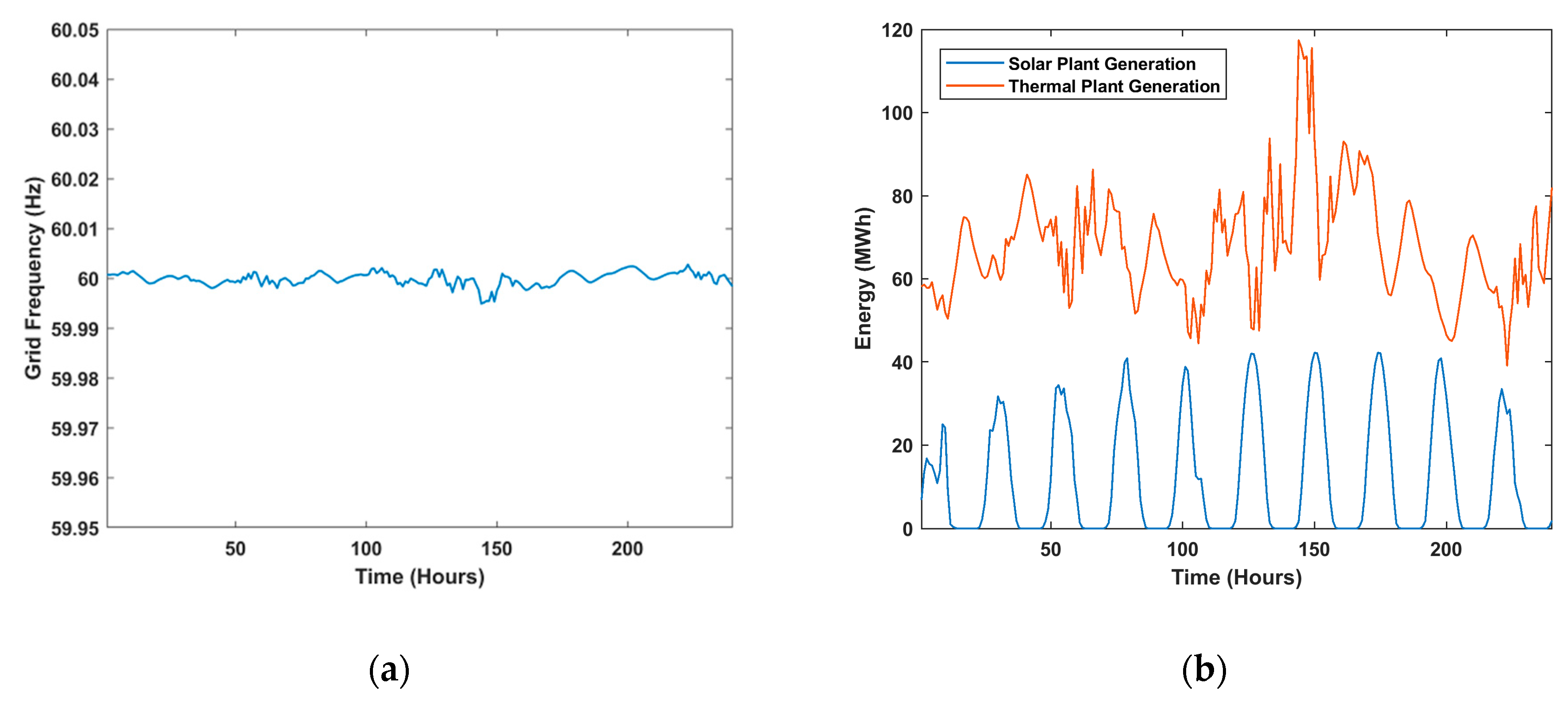
Figure 15 that the energy demand profile reaches negative values several times. This means that the grid is a net producing grid at these times. As mentioned earlier a PI controller for controlling the frequency of the grid has been tuned to avoid any complications in such cases. Figure 16 illustrates the frequency profile that corresponds to the energy demand profiles of Figure 15. Notice that the frequency has a slight increase at the times where the energy demand goes below zero, but still remains within safe operating conditions all the time.
To evaluate the models numerically, Table 2 shows the values of the coefficient of determination (R2), root mean squared error (RMSE), and normalized root mean squared error (NRMSE) for each model with the training and validation dataset and the testing datasets. The values shown for testing are the average values obtained from the ten testing datasets. Equations (14)–(16) were used to calculate R2, RMSE, and NRMSE, respectively.
R 2 = 1 i = 1 n ( y a c t u a l , i y m o d e l , i ) 2   i = 1 n ( y a c t u a l , i y ¯ ) 2
RMSE = i = 1 n ( y a c t u a l , i y m o d e l , i ) 2
NRMSE = RMSE y a c t u a l , m a x y a c t u a l , m i n
where y a c t u a l is the actual demand, y m o d e l is the model demand, y ¯ is the mean of the actual demand, y a c t u a l ,   m a x is the maximum value of the actual demand, and y a c t u a l , m i n is the minimum value of the actual demand.
From Table 2, it can be observed that the base case models completely failed, especially with the testing data. Notice that the base case N-ARXnet model has a negative testing R2 which illustrates how bad is this model. Also, L-ARX and N-ARX regression models have low performance. Interestingly, the two-step mechanisms for L-ARX and N-ARX regression have lower performance than the one-step mechanisms. On the contrary, the two-step mechanism N-ARXnet model has the best values for all metrics (highest R2 and lowest RMSE and NRMSE) as shown in bold in the table. This means that the two-step NARXnet model is the most trustworthy of all the models. However, the two-step models, in general, do not have a significant difference from the one-step models in terms of all the metrics. This is an important result as it means that the extra step of using the SOC in the calculations is not necessary to a certain extent, especially because using the SOC would require monitoring the battery usage of each house to collect training data. Therefore, considering the one-step models only, the N-ARXnet model is preferred as it has better performance (higher R2, lower RMSE, and NRMSE) than the other one-step models.
These results mean that with minimal information about the energy consumption within each house (only the battery SOC for the two-step mechanism) or with almost no information about it (the one-step mechanism), reliable data for the energy demand of the city can be predicted.

7. Conclusions and Future Work

The growing penetration of VREs is driving much technology development and deployment. Consumers at the residential level are incentivized to generate their power via rooftop PV. However, flat or simplified pricing structures give them no financial incentive to invest in storage or to pay any attention to when they use energy. While many regulatory would exist, this work has demonstrated that the introduction of variable pricing, combined with storage and proactive energy management systems would incentivize homeowners to invest in storage. This would allow them to respond to grid signals showing future pricing profiles and allow them to use these resources, in an automated way, to help alleviate some of the supply and demand mismatch issues that currently exist.
In this study, different machine learning models were developed for predicting the energy demand using only weather forecasts and electrical energy price profiles. The techniques used are L-ARX regression, N-ARX regression, and N-ARX neural network. The results showed that models with the two-step mechanism, which includes an intermediate step of predicting the total state of charge of the batteries, do not give significantly different results from the one-step model that predicts the energy demand in one-step. This justifies that the one-step models shall be preferred to avoid collecting SOC data for each house. Also, the base case models proved that using the electricity prices in the models is very important for catching all the changes that happen as the price varies.
A novel way for solving the complications that come with renewable penetration, as described in Section 4, is to set up an optimization problem incorporating the developed models in the structure of the problem (the objective function and the constraints), where the decision variables of the system would be the electricity prices. Building models that predict the energy demand with the electricity prices being the only decision variables are considered the main contribution of this study. In other words, the electricity prices can now be used to leverage electrical energy storage (ESS) and smart HVAC to regulate the operation of the grid and avoid most of its complications (e.g., complications resulting from the duck curve).
In future work, more rigorous ways for solving the problems related to smart grid operations, as discussed in Section 4, will be developed using stochastic optimization techniques instead of just using manual iterations. The results of these studies shall motivate policymakers in different countries to change the current electricity rate structures and to encourage homeowners to invest in smart home automation, including HVAC optimization and ESS.

Author Contributions

Conceptualization, M.S.; Methodology, M.S.; Formal analysis, M.S.; Writing-original draft preparation, M.S.; Writing-review & editing, K.P.; Supervision, K.P.; Project administration, K.P.

Funding

This research was funded by the Department of Energy–Office of Energy Efficiency and Renewable Energy Grant Number DE-EE0007712.

Conflicts of Interest

The authors declare no conflict of interest. The funder had no role in the design of the study; in the collection, analyses, or interpretation of data; in the writing of the manuscript, or in the decision to publish the results.

Nomenclature

Nomenclature
A Total thermal mass
B Overall heat transfer coefficient and surface area
C Constant term for neglected effects
f Frequency
P Power
Q Cooling energy
R Electricity price
S Absorbed solar radiation
T Temperature
t Time
W Weight
y Energy demand
Symbols
Δ Delta
η Efficiency
R 2 Coefficient of determination
τ Inertia of the grid
Subscripts
a m b Ambient
C Charging
D C Discharging
m a x Maximum
m i n Minimum
Abbreviations
AISArtificial immune system
ANNArtificial neural network
DSMDemand-side management
ESSEnergy storage system
GAGenetic algorithm
HVACHeating, ventilation, and air conditioning
L-ARXLinear autoregressive with exogenous inputs
N-ARXNonlinear autoregressive with exogenous inputs
N-ARXnetN-ARX neural network
NFNeuro-fuzzy
NRMSENormalized root mean squared error
PI controllerProportional-integral controller
PSOParticle swarm optimization
RMSERoot mean squared error
RTPReal-time pricing
SOCBattery state of charge
SVMSupport vector machine
VREVariable renewable energy

Appendix A. Solar Plant Model Equations

S = ( τ α ) n M [ G B R B K θ , B + G D K θ , D ( 1 + cos β 2 ) + G ρ G K θ , G ( 1 cos β 2 ) ]
where ( τ α ) n is the absorbed radiation at normal incidence and is calculated from the following equation [36]:
( τ α ) n = e K T G [ 1 ( n 1 n + 1 ) 2 ]
where “K” is the extinction coefficient, “ T G ” is the glazing thickness, and “n” is the refractive index and has typical values of 4 m−1, 2 mm, and 1.526 for PV systems, respectively.
M” is the air mass modifier and is calculated from the following correlation [36]:
M = α 0 + α 1 m + α 2 m 2 + α 3 m 3 + α 4 m 4
The constant α i has different values depending on the material of the solar panel. In this study, it is assumed that the panels are monocrystalline PV panels.
m” is called the air mass and is defined as the ratio of the mass of air that the beam radiation has to traverse at any given time and location to the mass of air that the beam radiation would traverse if the sun were directly overhead [36]. “m” can be calculated from the following relation [37]:
m = 1 cos Φ + 0.505 ( 96.08 Φ ) 1.634
where Φ is the solar zenith angle and is defined as the angle between the sun rays and the vertical to the earth’s center. Φ can be calculated from the following relation:
Φ = cos 1 ( sin L × sin δ + cos L cos δ cos h )
where “L” is the local latitude. For this study, the latitude for Salt Lake City, Utah is used. “ δ ” is the solar declination and is defined as the angular distance of the sun’s rays north or south of the equator. “h” is the hour angle.
δ ” can be calculated approximately by the following equation [38]:
δ = 23.45 × sin [ 360 365 ( 284 + N ) ]
where “N” is the day of the year.
h” can be calculated from the following equation:
h = ( A S T 12 ) × 15
AST” is the apparent solar time, which means that the hour angle is zero at local solar noon.
G B ” is the beam radiation or the direct normal irradiance which is obtained, for this study, from the TMY3 weather file for Salt Lake City, Utah.
G D ” is the diffuse radiation which is obtained from the TMY3 weather file for Salt Lake City, Utah as well.
G ” is the total irradiance which is the summation of G B and G D .
ρ G ” is the ground albedo which is the ratio of the radiation reflected from the surface to that incident on the surface. A typical value for PV panels is 0.2.
R B ” is the beam radiation tilt factor and is calculated from the following equation:
R B = cos θ
where “ θ ” is the incidence angle, which is defined as the angle between the sun’s rays and the normal to the surface of consideration which in this case is the solar panel. The incidence angle is calculated from the following equation [31]:
cos θ = sin L sin δ cos β cos L sin δ sin β cos Z s + cos L cos δ cos h cos β       + sin L cos δ cos h sin β cos Z s + cos δ sin h sin β sin Z s
where “ β ” is the surface tilt angle from the horizontal which is user-defined. For this study, the used value of “ β ” is 13 degrees. “ Z s ” is the surface azimuth angle which is the angle between the normal to the surface from true south which is user-defined. For this study, the used value of “ Z s ” is 26 degrees.
K θ , B , K θ , D , and K θ , G are the incidence angle modifiers for the beam, diffuse, and ground-reflected radiations, respectively, and are defined as the ratio of the radiation absorbed by the cell at incidence angle θ divided by the radiation absorbed by the cell at normal incidence.
The incidence angle modifiers are calculated from the following equations [36]:
K θ , B = ( τ α ) B ( τ α ) n
K θ , D = ( τ α ) D ( τ α ) n
K θ , G = ( τ α ) G ( τ α ) n
where ( τ α ) B , ( τ α ) D , and ( τ α ) G are the radiation absorbed by the cell through the beam, diffuse, and ground-reflected radiation, respectively. ( τ α ) B , ( τ α ) D , and ( τ α ) G can be calculated by the following equation [36]:
( τ α ) θ = e K L cos θ r [ 1 1 2 ( sin 2 ( θ r θ ) sin 2 ( θ r + θ ) + tan 2 ( θ r θ ) tan 2 ( θ r + θ ) ) ]
where θ r is the refraction angle and is calculated from the following relation:
θ r = sin 1 ( sin θ n )
For the diffuse radiation and the ground reflected radiation, an effective incidence angle is calculated for each from the following two correlations [39]:
θ e , D = 59.68 0.1388 β + 0.001497 β 2
θ e , G = 90 0.5788 β + 0.002693 β 2
where “ θ e , D ” is the effective incidence angle for diffuse radiation and “ θ e , G ” is the effective incidence angle from ground-reflected radiation.

References

  1. Fallah, S.; Deo, R.; Shojafar, M.; Conti, M.; Shamshirband, S. Computational intelligence approaches for energy load forecasting in smart energy management grids: State of the art, future challenges, and research directions. Energies 2018, 11, 596. [Google Scholar] [CrossRef]
  2. Gellings, C.W. Evolving practice of demand-side management. J. Mod. Power Syst. Clean Energy 2017, 5, 1–9. [Google Scholar] [CrossRef]
  3. Khemakhem, S.; Rekik, M.; Krichen, L. Impact of Electric Vehicles integration on residential demand response system to peak load minimizing in smart grid. In Proceedings of the 2019 19th International Conference on Sciences and Techniques of Automatic Control and Computer Engineering (STA), Sousse, Tunisia, 24–26 March 2019. [Google Scholar] [CrossRef]
  4. Wang, Y.; Yang, Z.; Mourshed, M.; Guo, Y.; Niu, Q.; Zhu, X. Demand side management of plug-in electric vehicles and coordinated unit commitment: A novel parallel competitive swarm optimization method. Energy Convers. Manag. 2019, 196, 935–949. [Google Scholar] [CrossRef]
  5. López, M.A.; De La Torre, S.; Martín, S.; Aguado, J.A. Demand-side management in smart grid operation considering electric vehicles load shifting and vehicle-to-grid support. Int. J. Electr. Power Energy Syst. 2015, 64, 689–698. [Google Scholar] [CrossRef]
  6. Sheha, M.N.; Powell, K.M. An economic and policy case for proactive home energy management systems with photovoltaics and batteries. Electr. J. 2019, 32, 6–12. [Google Scholar] [CrossRef]
  7. Zehir, M.A.; Ortac, K.B.; Gul, H.; Batman, A.; Aydin, Z.; Portela, J.C.; Soares, F.J.; Bargriyanik, M.; Kucuk, U. Development and field demonstration of a gamified residential demand management platform compatible with smart meters and building automation systems. Energies 2019, 12, 913. [Google Scholar] [CrossRef]
  8. Manganelli, M.; Greco, G.; Martirano, L. Design of a new architecture and simulation model for building automation towards nearly zero energy buildings. IEEE Trans. Ind. Appl. 2019, 55, 6999–7007. [Google Scholar] [CrossRef]
  9. Blackburn, L.; Young, A.; Rogers, P.; Hedengren, J.; Powell, K. Dynamic optimization of a district energy system with storage using a novel mixed-integer quadratic programming algorithm. Optim. Eng. 2019, 20, 575–603. [Google Scholar] [CrossRef]
  10. Kohlhepp, P.; Harb, H.; Wolisz, H.; Waczowicz, S.; Müller, D.; Hagenmeyer, V. Large-scale grid integration of residential thermal energy storages as demand-side flexibility resource: A review of international field studies. Renew. Sustain. Energy Rev. 2019, 101, 527–547. [Google Scholar] [CrossRef]
  11. Jabir, H.J.; Teh, J.; Ishak, D.; Abunima, H. Impacts of demand-side management on electrical power systems: A review. Energies 2018, 11, 1005. [Google Scholar] [CrossRef]
  12. Söder, L.; Lund, P.D.; Koduvere, H.; Bolkesjø, T.F.; Rossebø, G.H.; Rosenlund-Soysal, E.; Skytte, K.; Katz, J.; Blumberga, D. A review of demand side flexibility potential in Northern Europe. Renew. Sustain. Energy Rev. 2018, 91, 654–664. [Google Scholar] [CrossRef]
  13. Esther, B.P.; Kumar, K.S. A survey on residential Demand Side Management architecture, approaches, optimization models and methods. Renew. Sustain. Energy Rev. 2016, 59, 342–351. [Google Scholar] [CrossRef]
  14. Powell, K.M.; Sriprasad, A.; Cole, W.J.; Edgar, T.F. Heating, cooling, and electrical load forecasting for a large-scale district energy system. Energy 2014, 74, 877–885. [Google Scholar] [CrossRef]
  15. Muralitharan, K.; Sakthivel, R.; Vishnuvarthan, R. Neural network based optimization approach for energy demand prediction in smart grid. Neurocomputing 2018, 273, 199–208. [Google Scholar] [CrossRef]
  16. Reynolds, J.; Ahmad, M.W.; Rezgui, Y.; Hippolyte, J.L. Operational supply and demand optimisation of a multi-vector district energy system using artificial neural networks and a genetic algorithm. Appl. Energy 2019, 235, 699–713. [Google Scholar] [CrossRef]
  17. Cai, H.; Shen, S.; Lin, Q.; Li, X.; Xiao, H. Predicting the energy consumption of residential buildings for regional electricity supply-side and demand-side management. IEEE Access 2019, 7, 30386–30397. [Google Scholar] [CrossRef]
  18. Guo, Y.; Wang, J.; Chen, H.; Li, G.; Liu, J.; Xu, C.; Huang, Y. Machine learning-based thermal response time ahead energy demand prediction for building heating systems. Appl. Energy 2018, 221, 16–27. [Google Scholar] [CrossRef]
  19. Fan, C.; Xiao, F.; Wang, S. Development of prediction models for next-day building energy consumption and peak power demand using data mining techniques. Appl. Energy 2014, 127, 1–10. [Google Scholar] [CrossRef]
  20. Park, M.; Kim, J.; Won, D.; Kim, J. Development of a two-stage ESS-scheduling model for cost minimization using machine learning- based load prediction techniques. Processes 2019, 7, 370. [Google Scholar] [CrossRef]
  21. Mocanu, E.; Mocanu, D.C.; Nguyen, P.H.; Liotta, A.; Webber, M.E.; Gibescu, M.; Slootweg, J.G. On-line building energy optimization using deep reinforcement learning. IEEE Trans. Smart Grid 2019, 10, 3698–3708. [Google Scholar] [CrossRef]
  22. Mazidi, M.; Zakariazadeh, A.; Jadid, S.; Siano, P. Integrated scheduling of renewable generation and demand response programs in a microgrid. Energy Convers. Manag. 2014, 86, 1118–1127. [Google Scholar] [CrossRef]
  23. Vahedipour-Dahraie, M.; Najafi, H.; Anvari-Moghaddam, A.; Guerrero, J. Study of the effect of time-based rate demand response programs on stochastic day-ahead energy and reserve scheduling in islanded residential microgrids. Appl. Sci. 2017, 7, 378. [Google Scholar] [CrossRef]
  24. Yousefi, M.; Hajizadeh, A.; Soltani, M.N. A Comparison Study on Stochastic Modeling Methods for Home Energy Management Systems. IEEE Trans. Ind. Inform. 2019, 15, 4799–4808. [Google Scholar] [CrossRef]
  25. Cole, W.J.; Powell, K.M.; Hale, E.T.; Edgar, T.F. Reduced-order residential home modeling for model predictive control. Energy Build. 2014, 74, 69–77. [Google Scholar] [CrossRef]
  26. Cole, W.J.; Rhodes, J.D.; Gorman, W.; Perez, K.X.; Webber, M.E.; Edgar, T.F. Community-scale residential air conditioning control for effective grid management. Appl. Energy 2014, 130, 428–436. [Google Scholar] [CrossRef]
  27. Sheha, M.N.; Powell, K.M. Dynamic real-time optimization of air-conditioning systems in residential houses with a battery energy storage under different electricity pricing structures. Comput. Aided Chem. Eng. 2018, 44, 2527–2532. [Google Scholar]
  28. Sheha, M.N.; Rashid, K.; Powell, K.M. Dynamic real-time optimization of air conditioning systems in residential houses under different electricity pricing structures. In Proceedings of the 2018 American Control Conference, Milwaukee, WI, USA, 27 June–8 July 2018. [Google Scholar]
  29. Powerwall | The Tesla Home Battery. 2018. Available online: https://www.tesla.com/powerwall. (accessed on 1 June 2018).
  30. Residential Price Comparison. 2017. Available online: https://www.rockymountainpower.net/about/rar/rpc.html. (accessed on 24 September 2017).
  31. Duffie, J.A.; Beckman, W.A.; Worek, W.M. Solar Engineering of Thermal Processes; John Wiley & Sons, Inc.: Hoboken, NJ, USA, 2013. [Google Scholar] [CrossRef]
  32. This Duck Curve Is Solar Energy’s Greatest Challenge-Vox. Available online: https://www.vox.com/2018/5/9/17336330/duck-curve-solar-energy-supply-demand-problem-caiso-nrel (accessed on 3 December 2018).
  33. Ruiz, L.; Cuéllar, M.; Calvo-Flores, M.; Jiménez, M. An application of non-linear autoregressive neural networks to predict energy consumption in public buildings. Energies 2016, 9, 684. [Google Scholar] [CrossRef]
  34. Cox, S.J.; Kim, D.; Cho, H.; Mago, P. Real time optimal control of district cooling system with thermal energy storage using neural networks. Appl. Energy 2019, 238, 466–480. [Google Scholar] [CrossRef]
  35. Scapino, L.; Scapino, L.; Zondag, H.A.; Diriken, J.; Rindt, C.C.; Van Bael, J.; Sciacovelli, A. Modeling the performance of a sorption thermal energy storage reactor using artificial neural networks. Appl. Energy 2019, 253, 113525. [Google Scholar] [CrossRef]
  36. Kalogirou, S. Solar Energy Engineering Processes and Systems; Solar Energy Engineering; Elsevier Inc.: Amsterdam, The Netherlands, 2009. [Google Scholar]
  37. King, D.L.; Kratochvil, J.A.; Boyson, W.E. Field Experience with a New Performance Characterization Procedure for Photovoltaic Arrays; Sandia National Labs.: Albuquerque, NM, USA, 31 December 1997. [Google Scholar]
  38. ASHRAE Technical Committee. ASHRAE Handbook: Heating, Ventilating and Air-Conditioning Applications Inch-Pound Edition; ASHRAE Technical Committee: Atlanta, GA, USA, 2015. [Google Scholar]
  39. Brandemuehl, M.J.; Beckman, W.A. Transmission of diffuse radiation through CPC and flat plate collector glazings. Sol. Energy 1980, 24, 511–513. [Google Scholar] [CrossRef]
Figure 1. Schematic of the smart grid used in this study.
Processes 07 00870 g001
Figure 2. Grid operation flowchart.
Processes 07 00870 g002
Figure 3. A sample of four days of the real-time pricing profiles used for training, validation, and testing.
Processes 07 00870 g003
Figure 4. Smart house operation flowchart.
Processes 07 00870 g004
Figure 5. Frequency and generation results for 10 days. (a) A sample of 10 days for the grid frequency; (b) A sample of 10 days for the solar and thermal power generation.
Processes 07 00870 g005
Figure 6. Net energy demand at different levels of solar penetration.
Processes 07 00870 g006
Figure 7. Net demand with no price signals vs. optimized net demand with price signals.
Processes 07 00870 g007
Figure 8. Machine learning methods used in the study.
Processes 07 00870 g008
Figure 9. Prediction mechanisms.
Processes 07 00870 g009
Figure 10. A diagram for base case N-ARXnet structure for predicting energy demand.
Processes 07 00870 g010
Figure 11. A diagram for the N-ARXnet structure with one-step mechanism for predicting energy demand.
Processes 07 00870 g011
Figure 12. A diagram for the structure of the N-ARXnet two-step prediction model.
Processes 07 00870 g012
Figure 13. Some of the variables of the input dynamic model.
Processes 07 00870 g013
Figure 14. Parity plots of actual vs. predicted energy demand for the training dataset. (a) “Base case: no pricing used as inputs” L-ARX regression model; (b) one-step L-ARX regression model; (c) two-step L-ARX regression model; (d) one-step N-ARX regression model; (e) two-step N-ARX regression model; (f) “base case: No pricing used as inputs” N-ARXnet model; (g) one-step N-ARXnet model; (h) two-step N-ARXnet model.
Processes 07 00870 g014
Figure 15. Models validation against actual demand. (a) “Base case: no pricing used in inputs” L-ARX regression model; (b) One-step L-ARX regression model; (c) Two-step L-ARX regression model; (d) One-step N-ARX regression model; (e) Two-step N-ARX regression model; (f) “Base case: No pricing used in inputs” N-ARXnet model; (g) One-step N-ARXnet model; (h) Two-step N-ARXnet model.
Processes 07 00870 g015aProcesses 07 00870 g015b
Figure 16. Frequency profile that corresponds to the energy demand profile presented in Figure 15.
Processes 07 00870 g016
Table 1. Cost optimization equations.
Equation TypeExpression
Objective Function min i = 1 24 R i × ( Q i + P C i P D C i )
Temperature Equality Constraint T i + 1 ( A B Δ t ) = A T i + Δ t ( C B T h o u s e Q )
Battery Equality Constraint S O C i + 1 = S O C i + η C P C , i + 1 Δ t P D C , i + 1 η D C Δ t
Temperature Inequality Constraint T m i n < T i < T m a x
Cooling Energy Inequality Constraint 0 < Q i < Q m a x
Battery SOC Inequality Constraint 0 < S O C i < S O C m a x
Battery Charging Inequality Constraint 0 < P C i < P C m a x
Battery Discharging Inequality Constraint 0 < P D C i < P D C m a x
Table 2. Coefficient of determination (R2), root mean squared error (RMSE), and normalized root mean squared error (NRMSE) with the training and validation dataset vs. mean values with the ten testing datasets.
MethodMechanismEquation or StructureR2 Training and ValidationMean R2 TestingRMSE Training and ValidationMean RMSE TestingNRMSE Training and ValidationMean NRMSE Testing
L-ARX RegressionBase Case: No pricing used in inputsEquation (7)0.69960.070781.79142.850.09510.1650
One-StepEquation (8)0.79940.536266.84100.890.07770.1165
Two-StepEquations (9) and (10)0.80380.531866.11101.370.07690.1171
N-ARX RegressionOne-StepEquation (11)0.87470.574852.8396.560.06140.1116
Two-StepEquations (12) and (13)0.86550.575654.7296.510.06360.1115
N-ARX Neural NetworkBase Case: No pricing used in inputsFigure 100.7630−0.314371.00169.870.08160.1962
One-StepFigure 110.92550.634340.7389.590.04740.1035
Two-StepFigure 120.92950.683639.6283.300.04610.0962

