Proactive Energy Optimization in Residential Buildings with Weather and Market Forecasts


Abstract
1. Introduction
2. Previous Work
2.1. Grid Stabilization
2.2. Demand Side Management
2.3. Forecasting Methodology
2.4. Model Predictive Control in Building Energy Management
2.5. Accounting for Forecast Uncertainty and System Disturbances
2.6. Use of MHE in MPC
3. Contributions
- A home energy management system (HEMS) that uses a combined MHE and MPC approach that estimates residential home building parameters and optimizes home energy in real time. Mathematical building models are often very complicated and computationally expensive. This work overcomes this obstacle by using a lumped parameter model that is adapted to fit a high-fidelity model.
- A hybrid approach manages the on/off behavior of air conditioners as a continuous function using a mathematical program with complementarity constraints (MPCC). Discrete variables increase the number of potential solutions which require more computation resources and time. By using MPCC’s, the discrete behaviors are converted into a continuous function that is solved with continuous optimization.
- A combined renewable energy, energy storage, forecasts, cooling system, variable rate electricity plan, and multi-objective function residential house model is presented and tested on a simulated home in Phoenix, Arizona. This combination includes all major energy flows within a home as well as important outside disturbances. Accounting for these factors allows for a complete home energy optimization assessment with controlled conditions to assess the potential benefit from the HEMS approach.
4. Theory and Methods Used in Developing Energy Management Software
4.1. Methods
4.2. Theory/Overview
4.3. Simulation
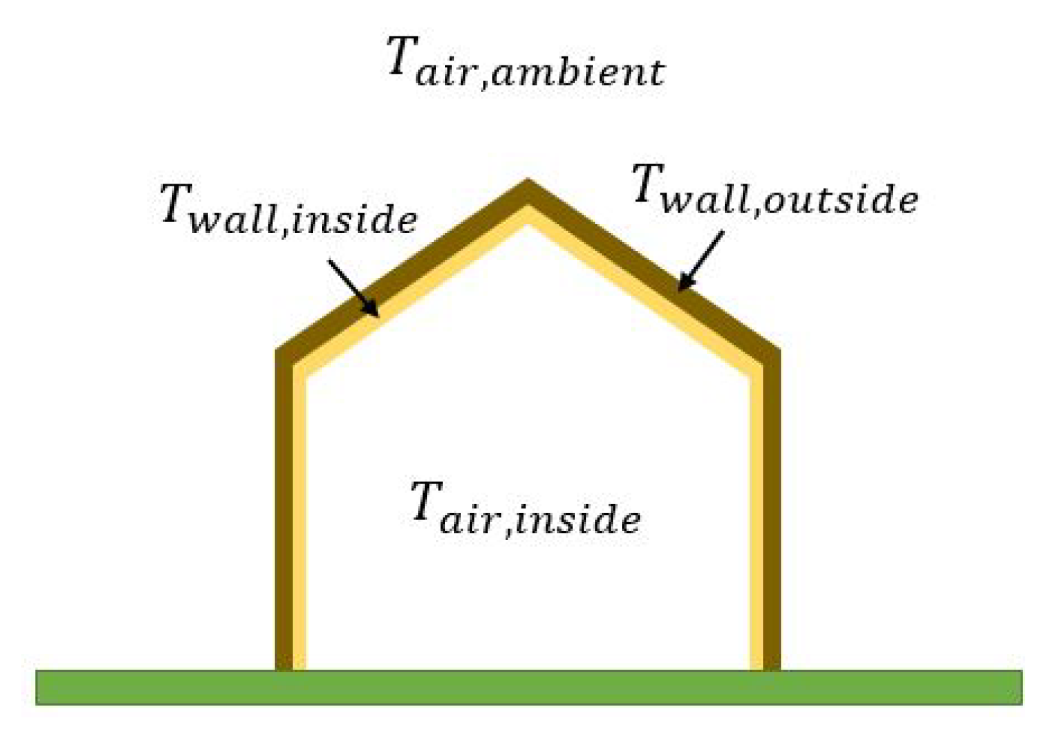
4.4. Building House Model
4.4.1. Initial Model
4.4.2. Improved Model
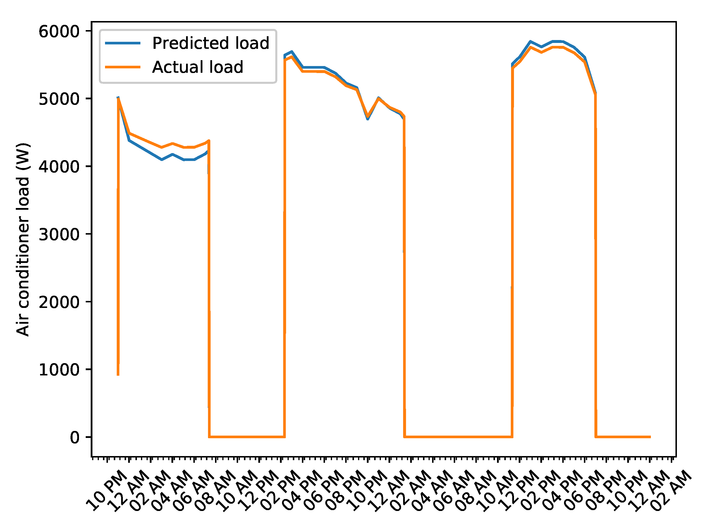
4.5. Air Conditioner Load Model
4.6. Battery Model
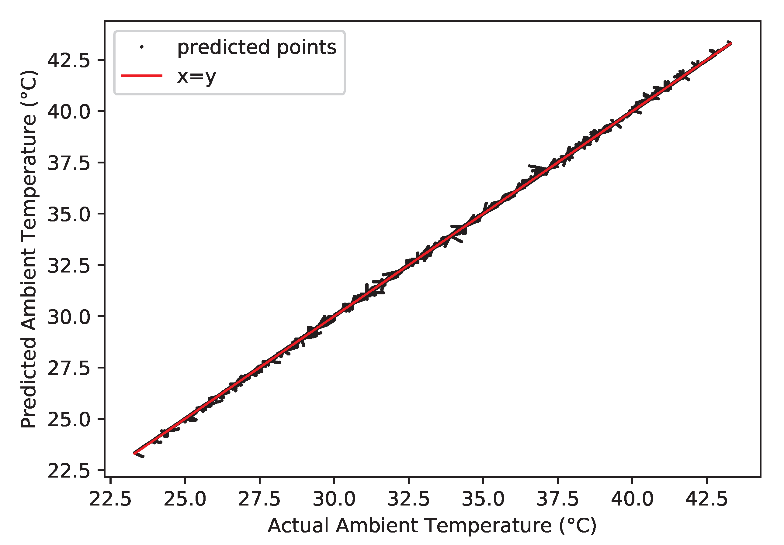
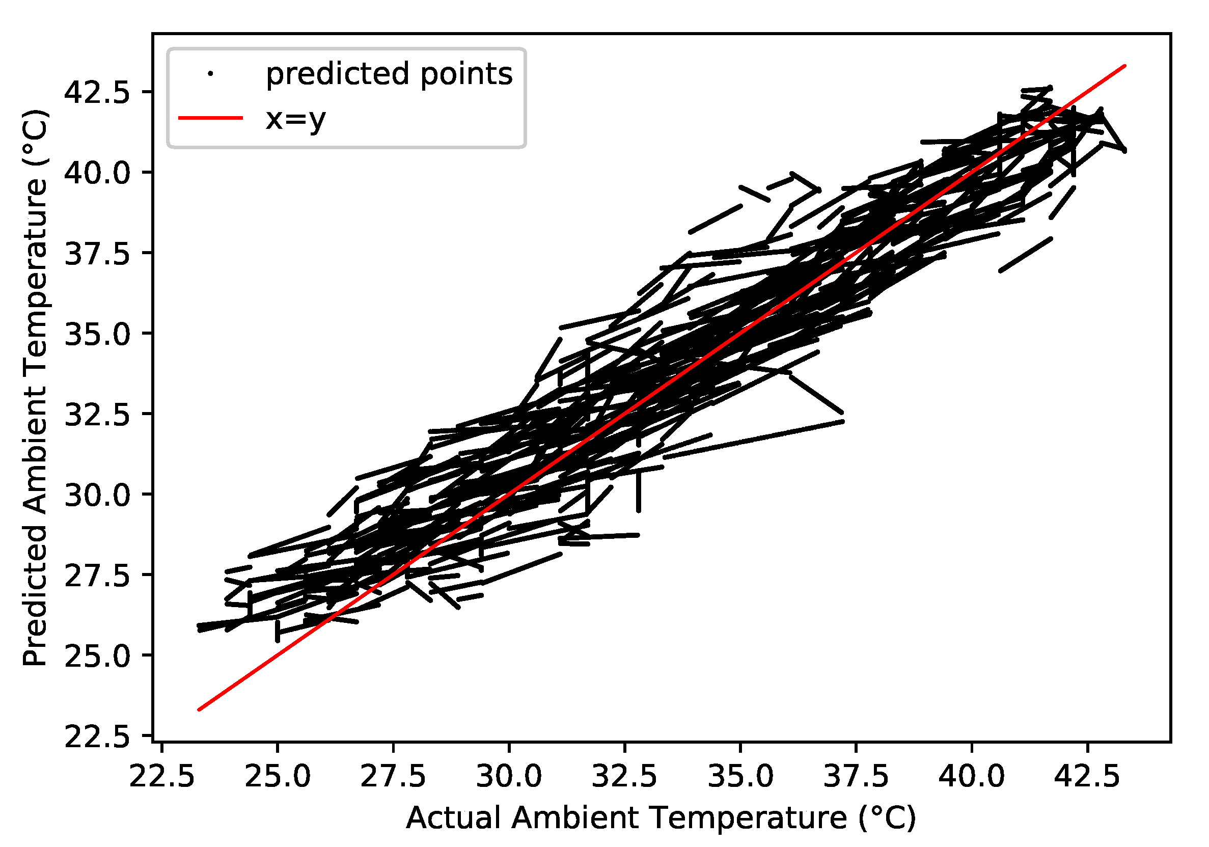
4.7. Ambient Temperature Prediction Model
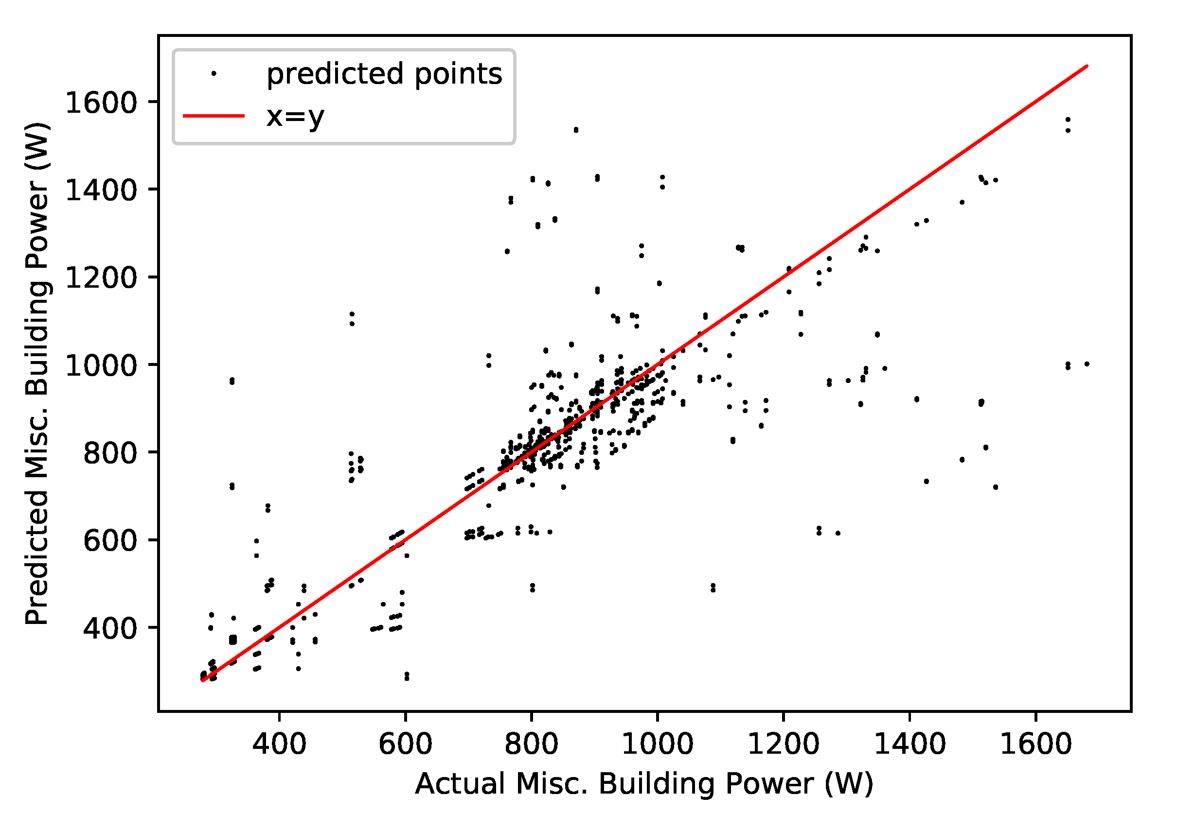
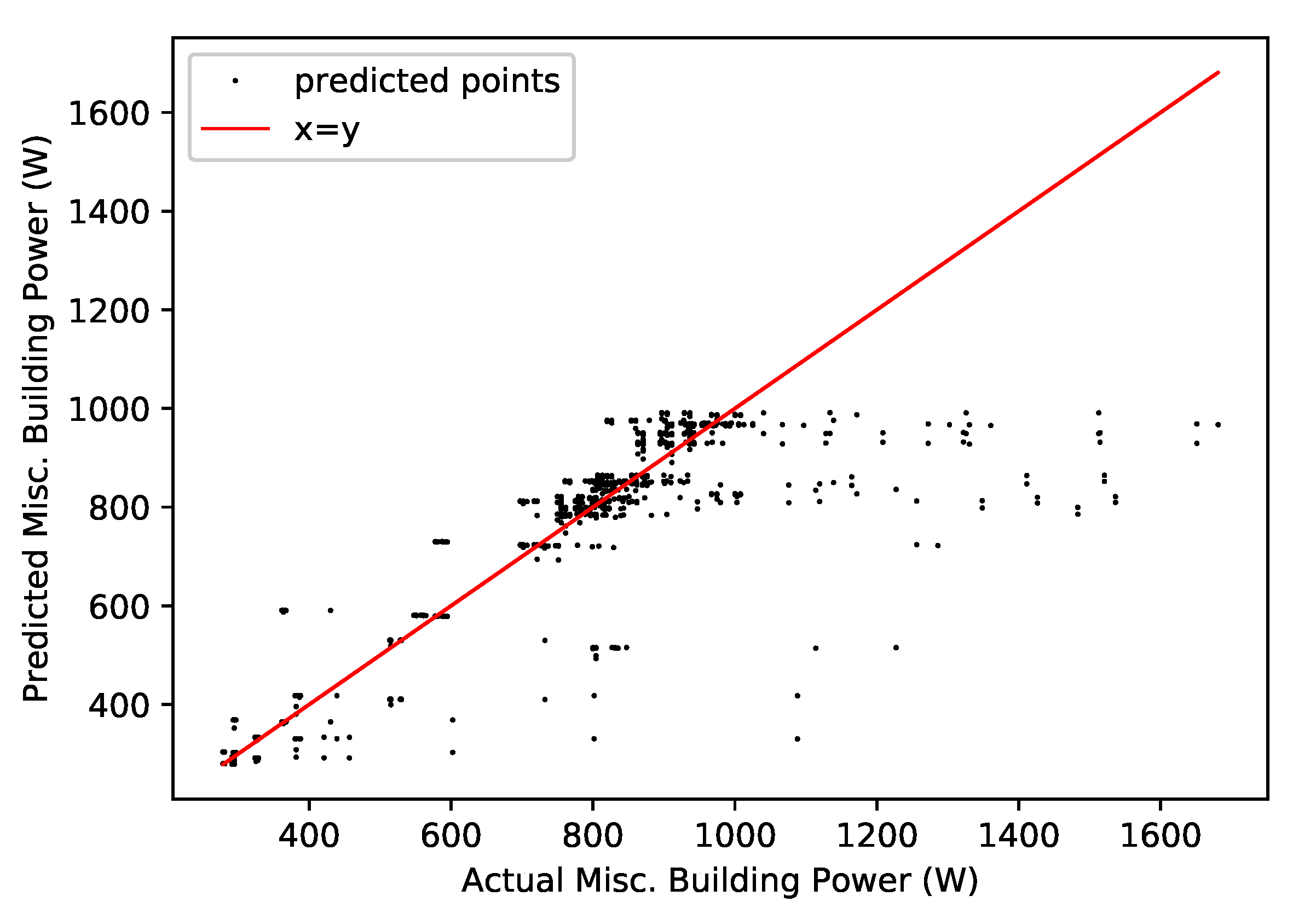
4.8. Miscellaneous Building Power Prediction Model
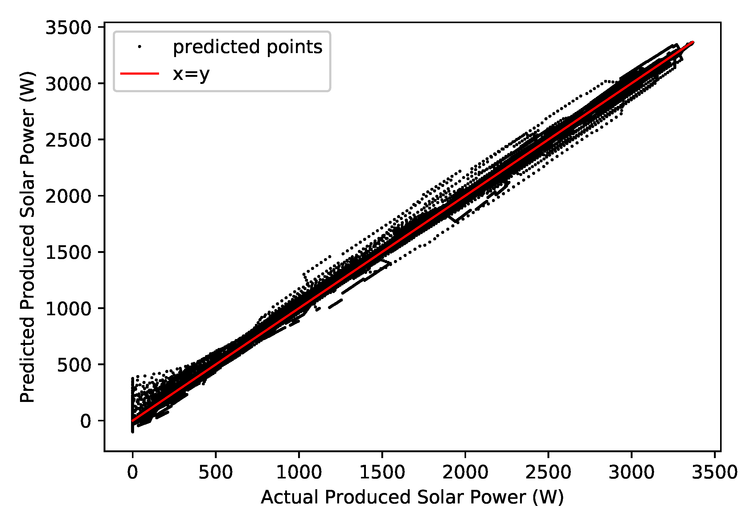
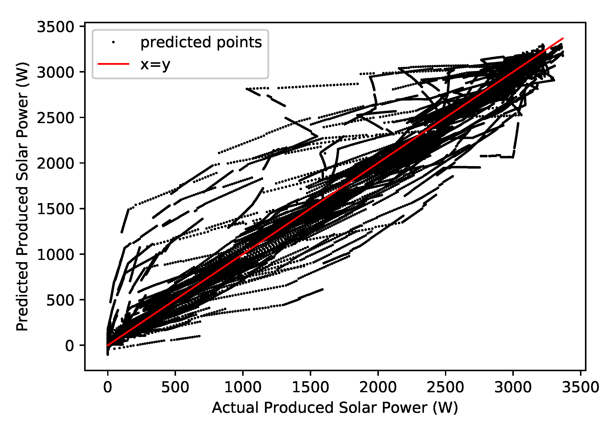
4.9. Solar Power Production Prediction Model
4.10. Moving Horizon Estimation and Model Predictive Control Theory
4.11. Moving Horizon Estimation with Lumped Parameters
4.12. Model Predictive Controller with Forecasts
5. Case Study Results
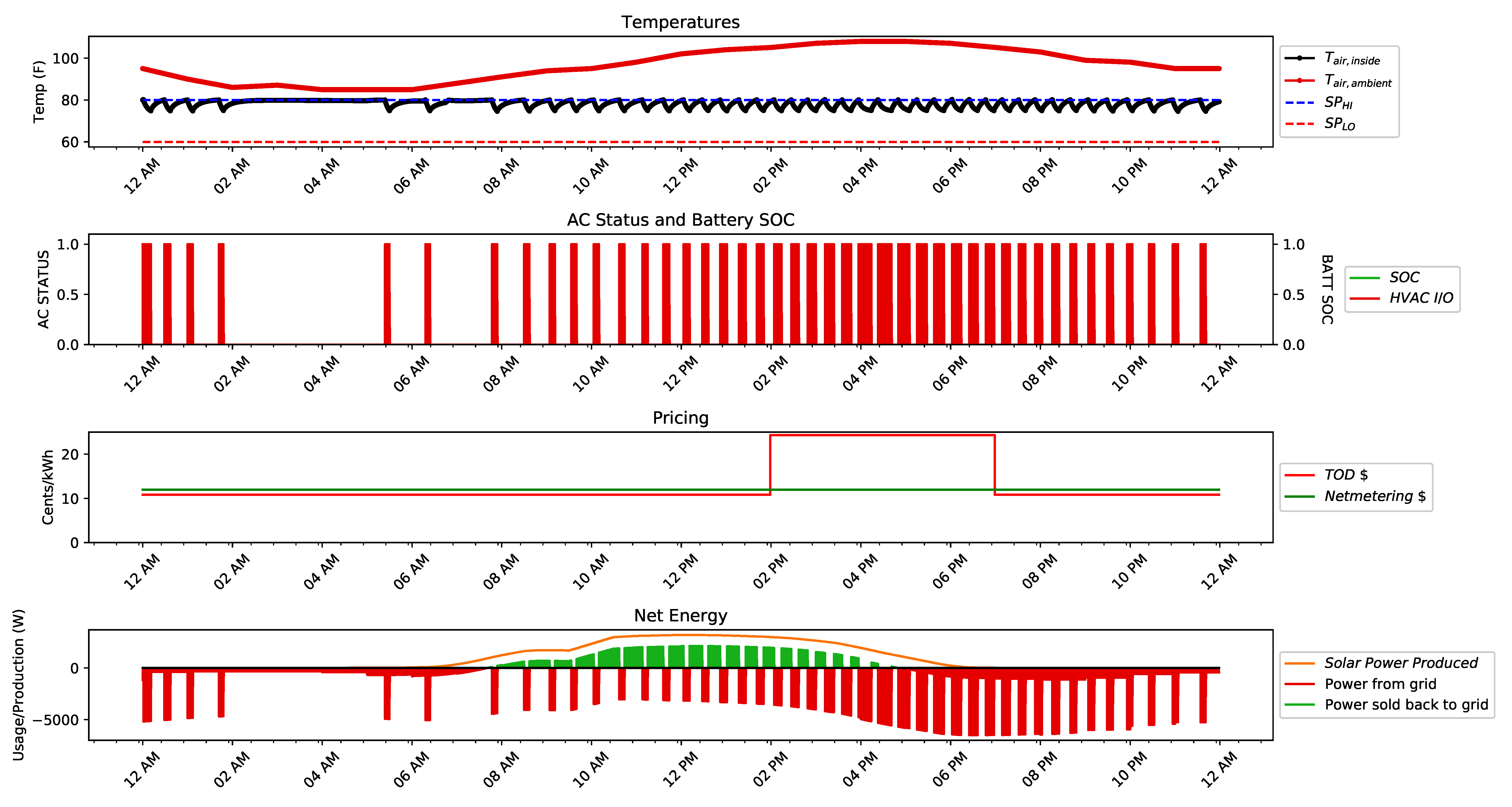
5.1. Base Case
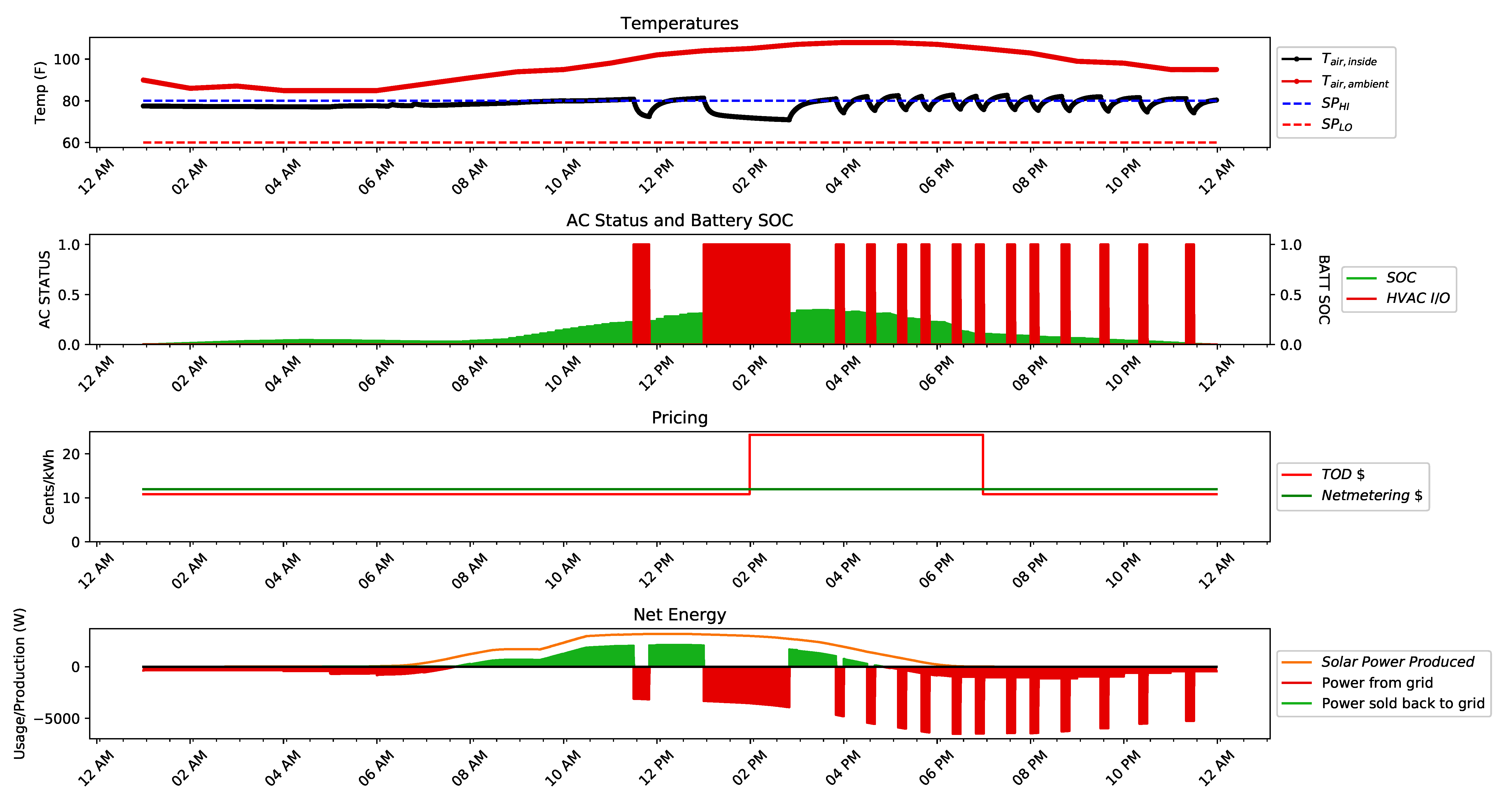
5.2. Optimized Case
5.3. Comparison to Base Case
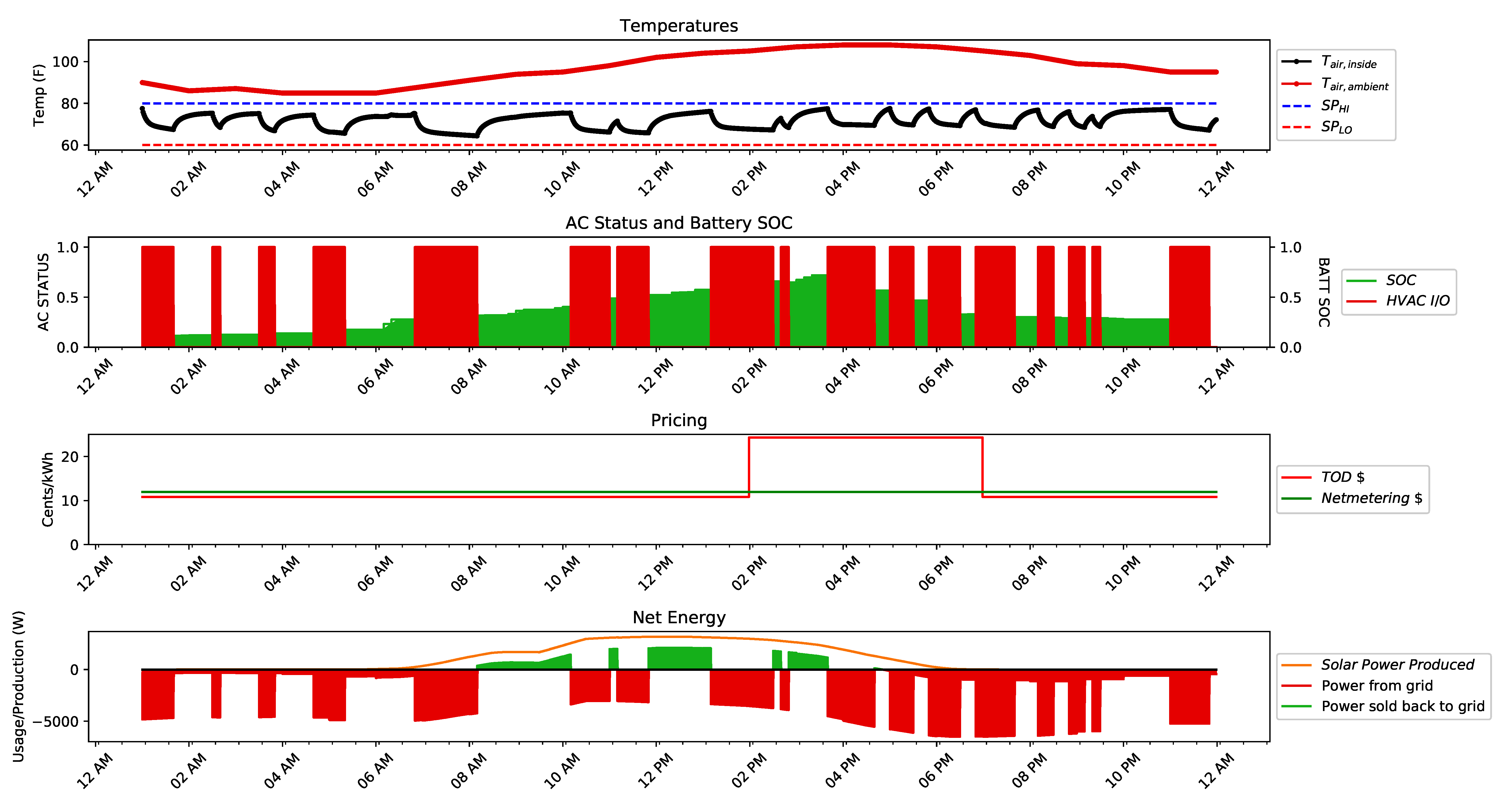
5.4. MPC Only HEMS Case Study
5.5. Comparison to Full HEMS Application
6. Conclusions and Future Work
Author Contributions
Funding
Acknowledgments
Conflicts of Interest
References
- IRENA. Renewable Energy Statistics 2019, 2019th ed.; IRENA: Abu Dhabi, UAE, 2019. [Google Scholar]
- IEA. Getting Wind and Sun onto the Grid. 2017. Available online: https://www.iea.org/publications/insights/insightpublications/Getting_Wind_and_sun.pdf (accessed on 18 April 2018).
- ISO. What the Duck Curve Tells Us about Managing a Green Grid. 2013. Available online: http://large.stanford.edu/courses/2015/ph240/burnett2/docs/flexible.pdf (accessed on 4 December 2019).
- SEIA. Utah State Solar Policy. 2017. Available online: http://www.seia.org/state-solar-policy/utah-solar (accessed on 12 June 2018).
- Powell, K.M.; Hedengren, J.D.; Edgar, T.F. Dynamic optimization of a solar thermal energy storage system over a 24 hour period using weather forecasts. In Proceedings of the 2013 American Control Conference, Washington, DC, USA, 17–19 June 2013; pp. 2946–2951. [Google Scholar] [CrossRef]
- Ahmad, T.; Chen, H.; Guo, Y.; Wang, J. Energy & Buildings A comprehensive overview on the data driven and large scale based approaches for forecasting of building energy demand: A review. Energy Build. 2018, 165, 301–320. [Google Scholar] [CrossRef]
- Anees, A.S. Grid integration of renewable energy sources: Challenges, issues and possible solutions. In Proceedings of the 2012 IEEE 5th India International Conference on Power Electronics (IICPE), Delhi, India, 6–8 December 2012; pp. 1–6. [Google Scholar] [CrossRef]
- Li, G.; Hwang, Y.; Radermacher, R.; Chun, H.H. Review of cold storage materials for subzero applications. Energy 2013, 51, 1–17. [Google Scholar] [CrossRef]
- Khan, A.R.; Mahmood, A.; Safdar, A.; Khan, Z.A.; Khan, N.A. Load forecasting, dynamic pricing and DSM in smart grid: A review. Renew. Sustain. Energy Rev. 2016, 54, 1311–1322. [Google Scholar] [CrossRef]
- Yoon, J.H.; Bladick, R.; Novoselac, A. Demand response for residential buildings based on dynamic price of electricity. Energy Build. 2014, 80, 531–541. [Google Scholar] [CrossRef]
- Sheha, M.N.; Powell, K.M. An economic and policy case for proactive home energy management systems with photovoltaics and batteries. Electr. J. 2019, 32, 6–12. [Google Scholar] [CrossRef]
- Aghaei, J.; Alizadeh, M.i. Demand response in smart electricity grids equipped with renewable energy sources: A review. Renew. Sustain. Energy Rev. 2013, 18, 64–72. [Google Scholar] [CrossRef]
- Good, N.; Ellis, K.A.; Mancarella, P. Review and classi fi cation of barriers and enablers of demand response in the smart grid. Renew. Sustain. Energy Rev. 2017, 72, 57–72. [Google Scholar] [CrossRef]
- Paterakis, N.G.; Erdinç, O.; Catalão, J.P.S. An overview of Demand Response: Key-elements and international experience. Renew. Sustain. Energy Rev. 2017, 69, 871–891. [Google Scholar] [CrossRef]
- Siano, P. Demand response and smart grids—A survey. Renew. Sustain. Energy Rev. 2014, 30, 461–478. [Google Scholar] [CrossRef]
- Shariatzadeh, F.; Mandal, P.; Srivastava, A.K. Demand response for sustainable energy systems: A review, application and implementation strategy. Renew. Sustain. Energy Rev. 2015, 45, 343–350. [Google Scholar] [CrossRef]
- Wang, J.; Zhong, H.; Ma, Z.; Xia, Q.; Kang, C. Review and prospect of integrated demand response in the multi-energy system. Appl. Energy 2017, 202, 772–782. [Google Scholar] [CrossRef]
- Brahman, F.; Honarmand, M.; Jadid, S. Optimal electrical and thermal energy management of a residential energy hub, integrating demand response and energy storage system. Energy Build. 2015, 90, 65–75. [Google Scholar] [CrossRef]
- O’Connell, N.; Pinson, P.; Madsen, H.; O’Malley, M. Benefits and challenges of electrical demand response: A critical review. Renew. Sustain. Energy Rev. 2014, 39, 686–699. [Google Scholar] [CrossRef]
- Pérez-Lombard, L.; Ortiz, J.; Pout, C. A review on buildings energy consumption information. Energy Build. 2008, 40, 394–398. [Google Scholar] [CrossRef]
- Lu, N.; Taylor, T.; Jiang, W.; Correia, J.; Leung, L.R.; Wong, P.C. The temperature sensitivity of the residential load and commercial building load. In Proceedings of the IEEE Power and Energy Society General Meeting, Calgary, AB, Canada, 26–30 July 2009; pp. 1–7. [Google Scholar] [CrossRef]
- Steinfeld, J.; Bruce, A.; Watt, M. Peak load characteristics of Sydney office buildings and policy recommendations for peak load reduction. Energy Build. 2011, 43, 2179–2187. [Google Scholar] [CrossRef]
- Zhao, H.X.; Magoulès, F. A review on the prediction of building energy consumption. Renew. Sustain. Energy Rev. 2012, 16, 3586–3592. [Google Scholar] [CrossRef]
- Yildiz, B.; Bilbao, J.I.; Sproul, A.B. A review and analysis of regression and machine learning models on commercial building electricity load forecasting. Renew. Sustain. Energy Rev. 2017, 73, 1104–1122. [Google Scholar] [CrossRef]
- Azhar, M.; Daut, M.; Yusri, M.; Abdullah, H. Building electrical energy consumption forecasting analysis using conventional and arti fi cial intelligence methods: A review. Renew. Sustain. Energy Rev. 2017, 70, 1108–1118. [Google Scholar] [CrossRef]
- Deb, C.; Zhang, F.; Yang, J.; Eang, S.; Wei, K. A review on time series forecasting techniques for building energy consumption. Renew. Sustain. Energy Rev. 2017, 74, 902–924. [Google Scholar] [CrossRef]
- Wei, Y.; Zhang, X.; Shi, Y.; Xia, L.; Pan, S.; Wu, J.; Han, M.; Zhao, X. A review of data-driven approaches for prediction and classification of building energy consumption. Renew. Sustain. Energy Rev. 2018, 82, 1027–1047. [Google Scholar] [CrossRef]
- Wang, Z.; Srinivasan, R.S. A review of arti fi cial intelligence based building energy use prediction: Contrasting the capabilities of single and ensemble prediction models. Renew. Sustain. Energy Rev. 2017, 75, 796–808. [Google Scholar] [CrossRef]
- Foucquier, A.; Robert, S.; Suard, F.; Stéphan, L.; Jay, A. State of the art in building modelling and energy performances prediction: A review. Renew. Sustain. Energy Rev. 2013, 23, 272–288. [Google Scholar] [CrossRef]
- Amasyali, K.; El-gohary, N.M. A review of data-driven building energy consumption prediction studies. Renew. Sustain. Energy Rev. 2018, 81, 1192–1205. [Google Scholar] [CrossRef]
- Fumo, N. A review on the basics of building energy estimation. Renew. Sustain. Energy Rev. 2014, 31, 53–60. [Google Scholar] [CrossRef]
- Lazos, D.; Sproul, A.B.; Kay, M. Optimisation of energy management in commercial buildings with weather forecasting inputs: A review. Renew. Sustain. Energy Rev. 2014, 39, 587–603. [Google Scholar] [CrossRef]
- Hedengren, J.; Asgharzadeh, R.; Powell, K.; Edgar, T. Nonlinear Modeling, Estimation and Predictive Control in APMonitor. Comput. Chem. Eng. 2014, 70, 133–148. [Google Scholar] [CrossRef]
- Beal, L.; Hill, D.; Martin, R.; Hedengren, J. GEKKO Optimization Suite. Processes 2018, 6, 106. [Google Scholar] [CrossRef]
- Yu, Z.; Huang, G.; Haghighat, F.; Li, H.; Zhang, G. Control strategies for integration of thermal energy storage into buildings: State-of-the-art review. Energy Build. 2015, 106, 203–215. [Google Scholar] [CrossRef]
- Afram, A.; Janabi-Sharifi, F. Theory and applications of HVAC control systems—A review of model predictive control (MPC). Build. Environ. 2014, 72, 343–355. [Google Scholar] [CrossRef]
- Killian, M.; Kozek, M. Ten questions concerning model predictive control for energy ef fi cient buildings. Build. Environ. 2016, 105, 403–412. [Google Scholar] [CrossRef]
- Serale, G.; Fiorentini, M.; Capozzoli, A.; Bernardini, D.; Bemporad, A. Model Predictive Control (MPC) for enhancing building and HVAC system energy efficiency: Problem formulation, applications and opportunities. Energies 2018, 11, 631. [Google Scholar] [CrossRef]
- Picard, D.; Drgoňa, J.; Kvasnica, M.; Helsen, L. Impact of the controller model complexity on model predictive control performance for buildings. Energy Build. 2017, 152, 739–751. [Google Scholar] [CrossRef]
- Ramos Ruiz, G.; Lucas Segarra, E.; Fernández Bandera, C. Model Predictive Control Optimization via Genetic Algorithm Using a Detailed Building Energy Model. Energies 2018, 12, 34. [Google Scholar] [CrossRef]
- Sangi, R.; Müller, D. A novel hybrid agent-based model predictive control for advanced building energy systems. Energy Convers. Manag. 2018, 178, 415–427. [Google Scholar] [CrossRef]
- Santoro, B.F.; Rincón, D.; da Silva, V.C.; Mendoza, D.F. Nonlinear model predictive control of a climatization system using rigorous nonlinear model. Comput. Chem. Eng. 2019. [Google Scholar] [CrossRef]
- Khakimova, A.; Kusatayeva, A.; Shamshimova, A.; Sharipova, D.; Bemporad, A.; Familiant, Y.; Shintemirov, A.; Ten, V.; Rubagotti, M. Optimal energy management of a small-size building via hybrid model predictive control. Energy Build. 2017, 140, 1–8. [Google Scholar] [CrossRef]
- Ascione, F.; Bianco, N.; De Stasio, C.; Mauro, G.M.; Vanoli, G.P. Simulation-based model predictive control by the multi-objective optimization of building energy performance and thermal comfort. Energy Build. 2016, 111, 131–144. [Google Scholar] [CrossRef]
- Oldewurtel, F.; Parisio, A.; Jones, C.N.; Gyalistras, D.; Gwerder, M.; Stauch, V.; Lehmann, B.; Morari, M. Use of model predictive control and weather forecasts for energy efficient building climate control. Energy Build. 2012, 45, 15–27. [Google Scholar] [CrossRef]
- Touretzky, C.R.; Baldea, M. Nonlinear model reduction and model predictive control of residential buildings with energy recovery. J. Process Control 2014, 24, 723–739. [Google Scholar] [CrossRef]
- Ryzhov, A.; Ouerdane, H.; Gryazina, E.; Bischi, A.; Turitsyn, K. Model predictive control of indoor microclimate: Existing building stock comfort improvement. Energy Convers. Manag. 2019, 179, 219–228. [Google Scholar] [CrossRef]
- Kwak, Y.; Huh, J.H.; Jang, C. Development of a model predictive control framework through real-time building energy management system data. Appl. Energy 2015, 155, 1–13. [Google Scholar] [CrossRef]
- Kim, S.H. Building demand-side control using thermal energy storage under uncertainty: An adaptive Multiple Model-based Predictive Control (MMPC) approach. Build. Environ. 2013, 67, 111–128. [Google Scholar] [CrossRef]
- Nojavan, S.; Zare, K. Stochastic optimization of energy hub operation with consideration of thermal energy market and demand response. Energy Convers. Manag. 2017, 145, 117–128. [Google Scholar] [CrossRef]
- Zhang, X.; Schildbach, G.; Sturzenegger, D.; Morari, M. Scenario-based MPC for energy-efficient building climate control under weather and occupancy uncertainty. In Proceedings of the European Control Conference (ECC), Zurich, Switzerland, 17–19 July 2013; pp. 1029–1034. [Google Scholar] [CrossRef]
- Kwak, Y.; Huh, J.H. Development of a method of real-time building energy simulation for efficient predictive control. Energy Convers. Manag. 2016, 113, 220–229. [Google Scholar] [CrossRef]
- Ebrahimpour, M.; Santoro, B.F. Moving Horizon Estimation of Lumped Load and Occupancy in Smart Buildings *. In Proceedings of the 2016 IEEE Conference on Control Applications (CCA), Buenos Aires, Argentina, 19–22 September 2016; pp. 468–473. [Google Scholar] [CrossRef]
- Copp, D.A.; Hespanha, J.P. Nonlinear output-feedback model predictive control with moving horizon estimation. In Proceedings of the 53rd IEEE Conference on Decision and Control, Los Angeles, CA, USA, 15–17 December 2014; pp. 3511–3517. [Google Scholar]
- Tenny, M.J.; Rawlings, J.B. Efficient moving horizon estimation and nonlinear model predictive control. In Proceedings of the 2002 American Control Conference (IEEE Cat. No. CH37301), Anchorage, AK, USA, 8–10 May 2002; Volume 6, pp. 4475–4480. [Google Scholar]
- Huang, R.; Biegler, L.T.; Patwardhan, S.C. Fast offset-free nonlinear model predictive control based on moving horizon estimation. Ind. Eng. Chem. Res. 2010, 49, 7882–7890. [Google Scholar] [CrossRef]
- Kraus, T.; Ferreau, H.J.; Kayacan, E.; Ramon, H.; De Baerdemaeker, J.; Diehl, M.; Saeys, W. Moving horizon estimation and nonlinear model predictive control for autonomous agricultural vehicles. Comput. Electron. Agric. 2013, 98, 25–33. [Google Scholar] [CrossRef]
- Joseph-Duran, B.; Ocampo-Martinez, C.; Cembrano, G. Output-feedback control of combined sewer networks through receding horizon control with moving horizon estimation. Water Resour. Res. 2015, 51, 8129–8145. [Google Scholar] [CrossRef]
- Copp, D.A.; Gondhalekar, R.; Hespanha, J.P. Simultaneous model predictive control and moving horizon estimation for blood glucose regulation in type 1 diabetes. Optim. Control Appl. Methods 2018, 39, 904–918. [Google Scholar] [CrossRef]
- Liang, X.; Li, Y.; Wu, X.; Shen, J. Nonlinear Modeling and Inferential Multi-Model Predictive Control of a Pulverizing System in a Coal-Fired Power Plant Based on Moving Horizon Estimation. Energies 2018, 11, 589. [Google Scholar] [CrossRef]
- Segovia, P.; Rajaoarisoa, L.; Nejjari, F.; Duviella, E.; Puig, V. Model predictive control and moving horizon estimation for water level regulation in inland waterways. J. Process Control 2019, 76, 1–14. [Google Scholar] [CrossRef]
- Beal, L.; Park, J.; Petersen, D.; Warnick, S.; Hedengren, J. Combined model predictive control and scheduling with dominant time constant compensation. Comput. Chem. Eng. 2017, 104. [Google Scholar] [CrossRef]
- Beal, L.; Petersen, D.; Grimsman, D.; Warnick, S.; Hedengren, J. Integrated scheduling and control in discrete-time with dynamic parameters and constraints. Comput. Chem. Eng. 2018, 115. [Google Scholar] [CrossRef]
- Beal, L.; Clark, J.; Anderson, M.; Warnick, S.; Hedengren, J. Combined Scheduling and Control with Diurnal Constraints and Costs using a Discrete Time Formulation. In Proceedings of the FOCAPO/CPC 2017, Foundations of Computer Aided Process Operations, Chemical Process Control; CACHE Corporation: Tucson, AZ, USA, 2017. [Google Scholar]
- Safdarnejad, S.M.; Hedengren, J.D.; Lewis, N.R.; Haseltine, E.L. Initialization strategies for optimization of dynamic systems. Comput. Chem. Eng. 2015, 78, 39–50. [Google Scholar] [CrossRef]
- Safdarnejad, S.M.; Gallacher, J.R.; Hedengren, J.D. Dynamic parameter estimation and optimization for batch distillation. Comput. Chem. Eng. 2016, 86, 18–32. [Google Scholar] [CrossRef]
- Safdarnejad, S.M.; Hedengren, J.D.; Baxter, L.L. Plant-level dynamic optimization of Cryogenic Carbon Capture with conventional and renewable power sources. Appl. Energy 2015, 149, 354–366. [Google Scholar] [CrossRef]
- Safdarnejad, S.; Kennington, L.; Baxter, L.; Hedengren, J. Investigating the Impact of Cryogenic Carbon Capture on Power Plant Performance. In Proceedings of the American Control Conference (ACC), Chicago, IL, USA, 1–3 July 2015; pp. 5016–5021. [Google Scholar] [CrossRef]
- Mojica, J.L.; Petersen, D.; Hansen, B.; Powell, K.M.; Hedengren, J.D. Optimal combined long-term facility design and short-term operational strategy for CHP capacity investments. Energy 2017, 118, 97–115. [Google Scholar] [CrossRef]
- Eaton, A.N.; Beal, L.D.; Thorpe, S.D.; Hubbell, C.B.; Hedengren, J.D.; Nybø, R.; Aghito, M. Real time model identification using multi-fidelity models in managed pressure drilling. Comput. Chem. Eng. 2017, 97, 76–84. [Google Scholar] [CrossRef]
- Eaton, A.N.; Beal, L.D.; Thorpe, S.D.; Janis, E.H.; Hubbell, C.; Hedengren, J.D.; Nybø, R.; Aghito, M.; Bjørkevoll, K.; Boubsi, R.E.; et al. Ensemble Model Predictive Control for Robust Automated Managed Pressure Drilling. In Proceedings of the SPE Annual Technical Conference and Exhibition; Society of Petroleum Engineers: Houston, TX, USA, 2015. [Google Scholar]
- Eaton, A.; Safdarnejad, S.; Hedengren, J.; Moffat, K.; Hubbell, C.; Brower, D.; Brower, A. Post-Installed Fiber Optic Pressure Sensors on Subsea Production Risers for Severe Slugging Control. In Proceedings of the ASME 34th International Conference on Ocean, Offshore, and Arctic Engineering (OMAE), St. John’s, NL, Canada, 31 May–5 June 2015. [Google Scholar]


| Property | Value |
|---|---|
| Battery Voltage | 50 V |
| Battery Usable Capacity | 13.5 kWh |
| Round Trip Efficiency | 90% |
| Maximum charge/discharge Power | 5 kW |
| Lithium-ion Cell Capacity | 1 Ah |
| Lithium-ion Cell Voltage | 3.6 V |
| Symbol | Description |
|---|---|
| Current In/Out of Battery | |
| Current In/Out of Cell | |
| Number of Cells in parallel | |
| Number of Cells in Series | |
| DC Power | |
| Efficiency of the Inverter | |
| AC Power | |
| Battery Voltage | |
| Cell Voltage | |
| Cell capacity discharged | |
| Battery capacity | |
| Cell capacity | |
| State of Charge of the Battery |
| Symbol | Description |
|---|---|
| objective function | |
| measurements | |
| y | model values |
| measurement deviation penalty | |
| penalty from the prior solution | |
| penalty from the prior parameter values | |
| dead band for noise rejection | |
| states , inputs , parameters , or disturbances | |
| change in parameters | |
| equation residuals, output fraction, and inequality constraints | |
| slack variable above and below dead-band measurement | |
| slack variable above and below a previous model value | |
| desired trajectory target or dead band | |
| penalty outside trajectory dead band | |
| cost of y, u and , respectively | |
| time constant of desired controlled variable response | |
| slack variable below or above the trajectory dead band | |
| target, lower, and upper bounds to final set-point dead band |
© 2019 by the authors. Licensee MDPI, Basel, Switzerland. This article is an open access article distributed under the terms and conditions of the Creative Commons Attribution (CC BY) license (http://creativecommons.org/licenses/by/4.0/).
Share and Cite
Simmons, C.R.; Arment, J.R.; Powell, K.M.; Hedengren, J.D. Proactive Energy Optimization in Residential Buildings with Weather and Market Forecasts. Processes 2019, 7, 929. https://doi.org/10.3390/pr7120929
Simmons CR, Arment JR, Powell KM, Hedengren JD. Proactive Energy Optimization in Residential Buildings with Weather and Market Forecasts. Processes. 2019; 7(12):929. https://doi.org/10.3390/pr7120929
Chicago/Turabian StyleSimmons, Cody R., Joshua R. Arment, Kody M. Powell, and John D. Hedengren. 2019. "Proactive Energy Optimization in Residential Buildings with Weather and Market Forecasts" Processes 7, no. 12: 929. https://doi.org/10.3390/pr7120929
APA StyleSimmons, C. R., Arment, J. R., Powell, K. M., & Hedengren, J. D. (2019). Proactive Energy Optimization in Residential Buildings with Weather and Market Forecasts. Processes, 7(12), 929. https://doi.org/10.3390/pr7120929