Abstract
An equilibrium model is applied to study the effect of forced temperature gradients introduced through heat exchange via specific segments of the wall of a chromatographic column operating with a liquid mobile phase. For illustration of the principle, the column is divided into two segments in such a manner that the first segment is kept at a fixed reference temperature, while the temperature of the second segment can be changed stepwise through fixed heating or cooling over the column wall to modulate the migration speeds of the solute concentration profiles. The method of characteristics is used to obtain the solution trajectories analytically. It is demonstrated that appropriate heating or cooling in the second segment can accelerate or decelerate the specific concentration profiles in order to improve certain performance criteria. The results obtained verify that the proposed analysis is well suited to evaluate the application of forced segmented temperature gradients. The suggested gradient procedure provides the potential to reduce the cycle time and, thus, improving the production rate of the chromatographic separation process compared to conventional isothermal (isocratic) operation.
1. Introduction
As binding of the solute by adsorption is an exothermic process and desorption is an endothermic process, migration speeds in chromatographic columns depend on temperature. Thermal effects are widely considered for gas phase flows through solid packings [1,2,3,4,5,6]. However, such effects are usually neglected in the liquid chromatography process (a) by considering the heat capacities of the two phases larger than the adsorption enthalpies and (b) by assuming a sufficiently larger value of the thermal conductivity to maintain a uniform temperature inside the column. As a result, most of the chromatographers have assumed isothermal conditions during the operation of liquid chromatography processes. However, there is experimental evidence of temperature fluctuations inside liquid chromatographic columns [7,8]. It has been found that temperature gradients broadly influence the production rate, yield and efficiency of the column. While, some studies show that they can reduce viscosity and can improve solubility and diffusivity [9,10]. Both separation and reactions are significantly affected by temperature fluctuations. Only a few contributions are available in the literature dealing with segmented temperature gradients in liquid chromatography [11,12,13,14,15,16,17,18,19]. One method implemented is temperature gradient interaction chromatography with triple detection (TGIC-TD). The method was suggested by Chang et al. to separate branched polymers according to their molecular weight with a high resolution [20,21,22,23].
In this study, a specific forced non-isothermal operation of a liquid chromatographic process is theoretically studied. Particularly, the internal temperature of the column is changed at a specific position through an external heating or cooling source fixed to the surface of the column wall. The heating accelerates and the cooling decelerates the migration speed of the fronts in specific regions of the column.
The current study is restricted to an equilibrium model, that is, axial dispersion of the concentration and temperature fronts are ignored. Equilibrium theory is very effective to design and analyze different complex processes. One of its powerful features is that it can successfully predict, tackle and explain the dynamic behavior of such complex processes. For comprehensive studies on equilibrium theory, see References [24,25,26]. In addition, it is further assumed that temperature changes in a forced stepwise manner uniformly inside the cross-sectional area of the column and no radial gradients occur. Thus, no energy balance is needed for the transport of heat through the column; instead, we provide temperature inside the column as a piece-wise step function.
The method of characteristics is utilized to solve the current model equations analytically. The method changes the original coordinate system to a new coordinate system in order to reduce the given partial differential equation (PDE) to an ordinary differential equation (ODE) along certain curves in the plane. Such curves, along which a given PDE reduces to an ODE, are called characteristic curves or just characteristics, which carry some information [27]. These curves are particularly relevant to the study of equilibrium theory discussed in this manuscript. Several case studies are conducted to quantify the influence of temperature gradients generated via an externally fixed source, production rate and yield of a chromatographic column.
The remaining parts of the paper are organized as follows. In Section 2, the non-isothermal chromatographic concept and model are introduced. In Section 3, the method of characteristic is applied to derive the solution trajectories and for performance evaluation, the production rate of the column is introduced. In Section 4, various scenarios are analyzed for illustration. Materials and methods used are given in Section 5 and conclusions are drawn in Section 6.
2. Non-Isothermal Equilibrium Model
We consider multi-component mixtures which are injected in a chromatographic column. The column is packed with spherical adsorbent particles. It is assumed that the bed is homogeneous and both axial and radial dispersion of the profiles are negligible. Furthermore, there is no interaction between the carrier fluid or solvent, and the solid phase and the composite fluid is assumed incompressible.
The considered equilibrium model deals with a fast rate of mass transfer and, as the name represents, it neglects molecular diffusion, axial dispersion and mass transfer resistances.
Let us consider concentrations for components, that are the functions of the spatial variable , which is taken as distance along the column of length , and time t. Here, denotes the arbitrary number of components. The concentrations are to be determined by mass balances. The concentrations of the adsorbed stationary phases are functions of the respective concentrations and the induced temperature T which are generally expressed in the form of functions, known as adsorption isotherms. Further, u represents the interstitial velocity which is assumed to be constant for all temperatures, and symbolizes the porosity of the bed. Both are constants. The balance law for a multi-component mixture in a volume element of the column mass is expressed as
For illustration of the wider applicable principle of segmented thermal gradients, we divide the z-domain just in two equal segments, from to , segment I, and from to , segment II. We consider that each of the segments behaves like an individual column and that the overall column is described by connecting these two segments. The outlet concentration profiles of segment I are the inlet concentration profiles for segment II. Hence, we define separate initial and boundary conditions for each segment and take care of conservation of masses in each segment separately.
Segment I is maintained at a fixed reference temperature, , while the temperature of segment II is changed uniformly via a fixed source placed at the outer surface of the conducting wall providing instantaneous heating, or cooling, , to the whole segment.
To illustrate the effect of the forced periodic regime, we illustrate in Figure 1 and Figure 2 three different scenarios. In the first scenario, c.f. Figure 1a, a single-solute pulse injection into the column is shown. Hereby, it is allowed to face, for example, a lower temperature in segment II. As the pulse starts crossing , its right part in segment II decelerates and its left part in segment I is still moving at the larger reference speed. As a result, the profile becomes narrower and more concentrated in segment II. After completely entering into segment II, the whole pulse is migrating at uniform low speed and reaches the column outlet. The second possible scenario is similar to the first one but now the pulse faces a higher temperature in segment II, see Figure 1b. As a result, an opposite effect is observed, that is, the pulse becomes broader and more diluted. A third possible scenario is more complicated and refers to the intrinsic goal of chromatography to separate components. For illustration, a three-component mixture is considered assuming that the first two components are migrating much faster than the third component (case “Late Eluter”), see Figure 2. Then, depending on the individual speeds, each component of the mixture faces the temperature changes at different times in segment II. Suitable changes in the temperature of segment II can improve separation performance, for example, production rate. For illustration, the mixture is injected periodically to the column both under isothermal and then non-isothermal conditions. Figure 2 reveals the potential to reduce the cycle time, that is, the time difference between two consecutive injections, in the non-isothermal case, , compared to the isothermal case, .
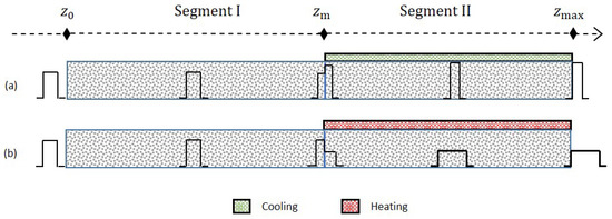
Figure 1.
Case (a) A single-solute pulse is injected one time into the column. The pulse is allowed to face a low temperature in segment II. As a result, the pulse becomes narrower and more concentrated. Case (b) Unlike case (b), the injected pulse faces a high temperature in segment II. Then, the pulse becomes broader and less concentrated.
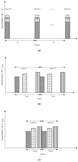
Figure 2.
(a) Illustration of a mixture of three components having three different Henry constants, periodically injected at . The cycle time is denoted by . (b) Effluent concentrations at for isothermal conditions and corresponding cycle time (case “Late Eluter”). In this case the retention times of the first two components are significantly smaller than the retention time of the third component. (c) The same mixtures are injected using suitable segmented temperature gradients (non-isothermal operation). The pulses then elute closer to each other, leading to a reduction in the cycle time, that is, .
Note that, another possible case “Early Eluter”, in which the first component is migrating much faster than the last two components, also exists but it is not illustrated below.
We formulate now mathematically, the exploitation of the temperature manipulation in segment II. A change in the temperature is performed when a certain pulse, completely or partially, crosses the point of the column. The resulting switching times for cooling or heating are denoted by for . Further let be the initial time and be the simulation time corresponding to each component i. To each semi-open interval for and , we associate a constant temperature for segment II of the column. We take a sequence , where are representing reference, low and high temperatures, respectively. With this, we define a first version of the temperature function for our theoretical experiment as
Note that in a general case, we will have to consider specific adjusted finite sequences of for each component of a mixture considering the specific migration and separation properties. Also the sequence of the switching times will depend on the specific migration speeds of the adsorption and desorption fronts.
The distribution equilibria of the components between the mobile phases and the solid phases under equilibrium conditions are described by a function, called, for a given constant temperature, adsorption isotherm. We apply a linear relation in concentration using temperature dependent Henry constants . This temperature dependence is expressed via Arhennius function incorporating the enthalpy of adsorption for each component i and the universal gas constant R. Thus the adsorption isotherm is linear in concentration and nonlinear in temperature, as expressed below
where is the Arhennius function depending upon T.
The columns (segments) are assumed to be fully regenerated. We inject concentration of component i for the duration of time . Let us denote the time in which the adsorption front of a pulse reaches by and the general cycle time between the injections by . Both will be calculated in Section 3. Then the initial and boundary conditions for segment I, processing number of injections, are given as
While for segment II holds
3. Analytical Solution
In this section we derive analytical expressions to quantify the transient concentration profiles, generally denoted by , under the influence of the described segmented temperature gradients. For this we first calculate the trajectories, . After dividing both sides of Equation (1) by and introducing the phase ratio , we obtain
By applying the chain rule over , we obtain
Since the temperature is constant in each segment, so and thus, the obtained value of from the above equation, when plug into Equation (6) yields
By Equation (3), . Plugging this value in Equation (7), after simplification, yields
Now, the method of characteristic is applied to reduce the above PDE to an ODE. As a result, analytical expressions for solution trajectories (paths) are obtained. According to Equation (8), the characteristic speed of the fronts corresponding to component i, using as a general time parameter, is given as
The solution of Equation (9) provides the trajectories of the solutions. Since the temperature is piece-wise constant, one can integrate this ODE easily. Further, we already know that and . For , Equation (9) gives
The above equation gives different space-time positions for each component. Using this equation, we can easily find the time :
For , we have . Now, the characteristics speed is affected by the temperature change. This effect depends on the particular switching time . Suppose that we have for some . This means that are the exploitable switching times in the interval . Note that these switching times may be different for different components i. Then, Equation (10) can be integrated as
The term , by setting , in the above equation tells that the temperature of the pulse stays still until the whole pulse enters segment II. This is possible when both the segments are initially kept at the same temperature. Later, in the case studies, we will discuss this scenario as a special case, c.f. Section 4.1, (Type II). We neglect this term for the case where both the segments are initially kept at different temperatures, c.f. Section 4.1, (Type I).
We denote the time dependent position of the adsorption (ad) front of the pulse by , while the position of the desorption (de) front by for component i. The adsorption front enters the column at while the desorption front enters at . With these initial times, the adsorption and desorption fronts can be explicitly determined. After a simple calculation, the characteristic curve or the space-time trajectory for is obtained from Equation (12) by taking again as
Further, we set and obtain for .
The above trajectories allow calculating the solution for the components’ concentration profiles as function of z and t. The solution consists of three parts divided in the time domain by a first state, , controlled by the reference temperature, a third (final) state, , controlled by a different temperature in segment II and an intermediate state, , which is influenced by both the temperatures via changing migration velocities, c.f. Figure 3. This later state gradually transforms the concentration in state , , to the concentration in state , , via the concentration in itself, . The concentration in each state depends on the difference between the trajectories of the adsorption and desorption fronts (space-bandwidths) in each state because it varies from state to state. Let be the space-bandwidth of the pulse in state , and be the space-bandwidth in state . These space-bandwidths are certainly constant because both adsorption and desorption fronts are migrating with same speeds in the corresponding states. But, the space-bandwidth in state is not constant because, in this state, the desorption front of the pulse is in segment I and the adsorption front is in segment II. So both are migrating with different speeds. As much as, the pulse enters segment II, the space-bandwidth in state tends to that in state . Let us denote this variable space-bandwidth by , c.f. Figure 4. Figure 3 and Figure 4 will be explained later to illustrate state graphically. We denote the part of in segment I, by and its part in segment II, by . Then and hence, by the conservation of mass, the concentration solutions in the states and are given as
and
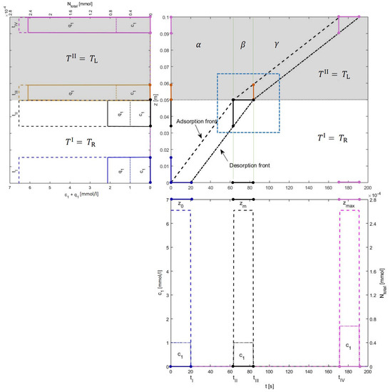
Figure 3.
Illustration of the solution behavior in and states for cooling of Type I: Switching is done from reference temperature, , to low temperature, . Concentrations, associated with left axes, are plotted along the axial coordinate z at particular times inside the column and plotted against the time coordinate t at different locations in the column. The total mass, , associated with the right axes of z-plot and t-plot, are also plotted to guarantee the mass balance. The grey area represents segment II that is kept at a low temperature. Every point in the t-plot corresponds to two points in the z-plot and every point in the z-plot corresponds to two points in the t-plot. The blue profile in t-plot is showing the reaching times of the adsorption and desorption fronts to . Corresponding to it is a blue profile in z-plot at . The black profile in t-plot is showing the profile when the fronts reach . This crossing is plotted in the z-plot at several positions, that is, black one when the adsorption front reaches and orange one when the desorption front reaches . The pink profile in the t-plot is plotted at . Whereas, the pink profile in the z-plot illustrates the situation when the adsorption front reaches . As is the crucial state, we have marked the area covering this sate and shown it in Figure 4 to delve the transition more clearly.
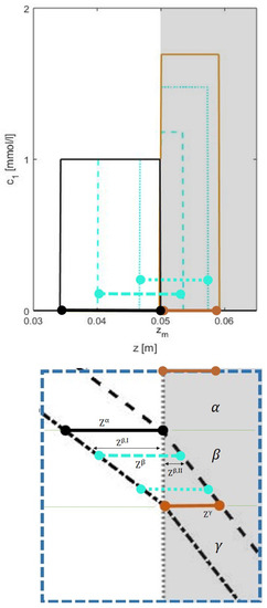
Figure 4.
Illustration of the solution behavior in the intermediate state for cooling of Type I: The state , highlighted by blue colored dashed boundary in Figure 3, is rotated clockwise along with the corresponding portion of the z-plot. The pulse is shown at two places by cyan color, using dashed line when most of its part is in segment I and, by dotted line when most of its part is in segment II. As the sapce-bandwith gradually changes in state , the corresponding concentration also changes accordingly. All the space-bandwidths (, , , ) can be calculated using Equation (13).
The main aim of the temperature gradients being analyzed in this article is to enhance the production rate, , which is defined at the end of this section (Equations (20) and (21)). This can be achieved by reducing the cycle time, c.f. Figure 2. In Section 4.2, we particularly calculate a cycle time with a conservative limit. We consider that a new injection should be introduced in such a way that the adsorption front of its fastest component reaches the middle of the column, , at the same time as the desorption front of the slowest component of the previous injection leaves the column. Exactly at this time we switch the temperature of segment II back to its initial value and repeat the same sequence shifted by the cycle time. To calculate the cycle time denoted generally by , we use Equation (13). Let be the time taken by the desorption front of the slowest component of the previous injection having Henry constant, say , to reach . Then the expression for in terms of , taking , is given as
After simplification, we get the value of the time as
On the other hand, the time , in which the adsorption front of the fastest component of the next injection, having Henry constant, say , covers the distance , is the same as for the fastest component of previous injection, and is given by Equation (11) as
Then, the cycle time is given as
Equation (19) can be used to calculate the cycle times and for both isothermal and the more flexible non-isothermal conditions, respectively, because .
Performance of the Chromatographic Process
In chromatography, the production rate of the column is defined to be total mass of each component per cycle time. Most important to quantify preparative chromatography is to identify the shorter possible cycle time. To see the improvement in the production rates, we compare the production rate of the column under non-isothermal conditions, P, with the production rate of the column under isothermal conditions, P. If N is the mass of each component migrating from the column inlet to the column outlet, is the cycle time in the non-isothermal case, is the cycle time in the isothermal case and A is the cross-sectional area of the column, then both the production rates can be written mathematically as
and
where, for some and , we have
From both the Equations (20) and (21), it is obvious that the process with shorter cycle time will have higher production rate. The total mass collected at the outlet of the column can reach the injected amount if there is no overlap between the eluting bands (N). Only this attractive scenario is considered below.
Since we consider in this paper, the same column volume both in isothermal and non-isothermal operations, we do not touch here the scale dependent aspect, that is typically used to evaluate a productivity as the ratio of production rate over column dimension.
4. Illustration and Discussion of Results
After deriving analytical solutions, we evaluate case studies for three different scenarios discussed in Figure 1 and Figure 2. Based on first switching time of the temperature, we also discuss one special case, c.f. Section 4.1, (Type II). In the considered case studies, the number of components in the mixture is either 1 or 3. The parameters used in the simulation for all cases are listed in Table 1 and Table 2. They represent typical values that describe separations performed using liquid chromatography.

Table 1.
Reference parameters used in Section 4.1 (single-component injection).
Table 2.
Reference parameters used in Section 4.2 (Consecutive injections of multicomponent mixtures).
4.1. Analysis of Single-Component Injection
As explained in Figure 1a,b, we first test our analytical solutions for the case of only one single-component injection () which is injected as a rectangular pulse at the column inlet. After reaching the middle of the column, it faces a temperature change. It could be a low or high temperature as explained in Figure 1a,b, and in the special case, discussed above, it could be reference temperature for a short time, c.f. Equation (2). In practice, there are two possible ways for the pulse to be effected by a temperature change in segment II of the column.
Type I: Both segments are initially at different temperatures
In this case, segment I of the column has the reference temperature and segment II is maintained either at uniform low or high temperature, that is, and or . As the adsorption front starts crossing the middle of the column, , it faces two different temperatures before completely entering segment II, that is, speeds of both the fronts of the pulse are not the same. Figure 3 and Figure 4 demonstrate the experiment for low temperature, and Figure 5 depicts the experiment for high temperature, , in segment II. In this case, Equation (13) takes the form
While, the concentration profiles are given by Equations (14) and (15) by just puting .
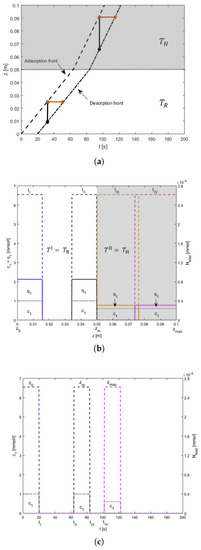
Figure 5.
Illustration of the solution behavior for heating of Type I: Concentrations are plotted along the left axes and the total mass of the component, , showing the achievement of mass conservation, is plotted along the right axes of z-plot and t-plot. Segment II is kept at a high temperature. (a) The pulse is accelerated but in segment II, space-bandwidths become broader as compared to segment I. The time-bandwidth stays the same as in the previous case. (b) The blue color is showing the position of the pulse at , in black color, when its adsorption front reaches , in orange color, when its desorption front reaches and it is plotted in pink color when its adsorption front reaches . (c) The blue color profile is showing the arrival times of both the fronts at , black color, when they reach and the pink color profile is showing when they reach .
All the solutions are plotted in Figure 3, Figure 4 and Figure 5. The concentration profiles are plotted along the z-coordinate of the column at specific times and along t-coordinate, they are plotted at different locations, including the most important positions and . We call the development of the concentration profiles in time as “t-plot” and in space as “z-plot”. The plot of space-time trajectories is also given in the middle of the Figure 3 where all the three states and (discussed in Section 3) are mentioned. To demonstrate the matching of space-bandwidths and time-bandwidths, z-plot is placed on the left and t-plot is placed below the plot of space-time trajectories. State is highlighted and demonstrated separately in Figure 4. In Figure 3, the z-plot shows that across z, the space-bandwidth changes but across t the time-bandwidth between both fronts stays the same. The reason for this is that, although the space-bandwidths between the fronts vary, their speeds also change accordingly. For example in the z-plot given in Figure 3, the space-bandwidth between the fronts decreases and the profile becomes more concentrated. It causes an decrease in the time-bandwidth, but, meanwhile, the speeds of the fronts are also decreased and this smooths the change in the time-bandwidth. So the time-bandwidth inside the two segments stays the same. See t-plot in Figure 3. Figure 5 tells us the similar story, which is plotted for the higher temperature in segment II. In this case, in place of narrowing, the space-bandwidth becomes broader and the profile becomes less concentrated. in segment II of the column.
Type II: Both segments are initially at the same temperature
This special case is discussed to support the understanding of more complex front propagation of mixtures (c.f. Section 4.2). Here, segment II is initially at the reference temperature. The temperature changes only when the pulse completely enters this segment, that is, when the desorption front of the pulse also crosses . In this case, and . Thus, unlike the previous case, both fronts of the pulse are moving under the influence of the same temperature during its migration in segment II of the column. In other words, the migration speeds of both fronts are the same and, hence, the space-bandwidth of the pulse is not altering. Figure 6 displays the experiment for both the temperatures and . Here, the characteristics given by Equation (13), taking , take the form
Whereas, all other solutions remain the same.
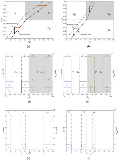
Figure 6.
Illustration of the solution behavior for both cooling and heating of Type II: Concentrations and mass are again plotted along the left and right axes, respectively. (a) The grey color is representing segment II with low temperature. The temperature is switched from reference to low at time when the desorption front of the pulse also enters segment II. The space-bandwidth is marked by black color and stays unchanged. The time-bandwidth of the pulse is marked by orange color which becomes longer. (b) Here, the grey color is representing segment II with high temperature. Unlike case (a), here the time-bandwidth decreases. (c,d) are z-plots for cooling and heating respectively. Whereas. (e,f) are t-plots for cooling and heating respectively.
Figure 6a,b show that across , unlike the previous case, the space-bandwidths of the profile do not change but the time-bandwidths do, that is, duration between the fronts changes in the time domain. This is due to the fact that both fronts are experiencing the same temperature at the same time and, thus, their speeds change at the same time. This does not allow any change in the space-bandwidths but this allows a change in the time-bandwidth. The graphical results are displayed in Figure 6c–f.
4.2. Analysis of Consecutive Injections of Multicomponent Mixtures
After single-solute injections, we extend our analysis to mixtures of three components (case “Late Eluter”), which can be under isothermal conditions but less productive, c.f. Figure 2. Now we want to exploit forced temperature modulation of segment II to achieve improvements shown in Figure 2.
Let be the solution trajectories of the adsorption fronts of component 1 (fastest one), component 2 (middle one) and component 3 (slowest one). Then the trajectories of all the three components for the first injection, in view of Equation (13), are given as
Equations (25)–(27) also describe the trajectories for the desorption fronts of all the three components as given by Equation (13) as well as the trajectories of the components of the mixtures injected later. The concentration solution for all the components of the mixtures are given by Equations (14) and (15). The resulting values are given by Table 3. Note that in case of isothermal operation, the temperatures can be replaced by the reference temperature everywhere in above equations to get the solution trajectories. All the trajectories are plotted for multiple injections in Figure 7.
Table 3.
Results for Section 4.2 (Consecutive injections of multicomponent mixtures).
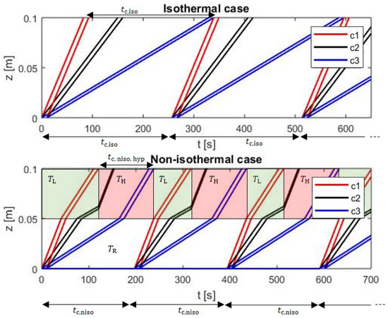
Figure 7.
The space-time trajectories for three components under isothermal (3 injections) and the non-isothermal (4 injections) conditions. In the non-isothermal case, the first switching of the temperature is done at and second switching at and then they shift by alternatively.
The top part of Figure 7 shows, for three feed components, the optimal development of the concentration profiles for the conventional isothermal (isocratic) case. The minimal cycle time, which corresponds to the highest production rate (Equations (20) and (21)), is the difference between the time, , when the desorption front of component 3 and the time, , when adsorption front of component 1 leave the column under isothermal conditions. Both the times can be easily calculated using the equations above by using the temperature everywhere. This cycle time, which is 257 s for the parameters used, guarantees that there is no overlap between consecutive cycles and no waste of time by waiting too long before injecting again.
The lower part of Figure 7 illustrates a situation exploiting the forced periodic temperature modulation in segment II. The initial temperature of the segment II, which is set in the figure to be , does not play a role before the first component arrives. In order to reduce the cycle time, it is desirable to decelerate component 1 and to accelerate component 3 and hence one can see, the temperature in the trajectories of component 1 and in the trajectories of component 3 given by Equations (25) and (27). With this, component 2 also decelerates first (by temperature faced by component 1) and then accelerates (by temperature faced by component 3), due to its presence in the temperature zones associated with component 1 and component 3, at different times, respectively, c.f. Equation (26). A hypothetical time limit, , is again given by the difference between the time when the desorption front of component 3 (now earlier than in the isothermal case) and the time when the adsorption front of component 1 (now later than in the isothermal case) leave the column. In the particular case studied, this leads to = 129 s. If this shortest hypothetical cycle time is applied, there is the danger that also the bands of component 1 and component 3 could be bend a second time in segment II, which can cause unwanted remixing. For this reason the figure illustrates a sample to apply conservative temperature switching regime, which avoids this remixing and still guarantees that the cycle time in the non-isothermal case is shorter than in the isothermal case. This strategy is based on switching in the segment II, the temperature from high to low and back from low to high at the times, when the adsorption front of component 1 enters this segment (for the first time at = 41 s) and the time when this component finally leaves the column (for the first time at = 120 s), respectively. Note that the later mentioned time is now different than that in isothermal case. The temperature switching now occur periodically, shifted just by cycle time . Application of this suitable strategy leads to = 197 s, which corresponds to a production rate increase compared to the isothermal case of 30% (see also Table 3). It should be noted here that this conservative temperature modulation strategy does not present an optimum for the segmented non-isothermal case. Such a case dependent optimal situation could be identified based on the specific concentration trajectories described by the analytical solutions given by above three equations. It would cause a more frequent temperature switching. The solution of such a challenging optimization problem was not considered here.
5. Materials and Methods
The analytical expression of the solutions are already presented in the above sections. These solutions were implemented in the MATLAB software and these programs will be freely available in the library of Max Planck Institute for Dynamics of Complex Technical Systems Magdeburg, Germany.
6. Conclusions
Equilibrium theory and the method of characteristics were used to derive analytical solutions for the trajectories of elution profiles of forced temperature gradient chromatography analytically. Two segments of the column are considered. In the second segment, temperature was modulated. The profiles in the intermediate section around the perturbation point are delved deeper to guarantee the conservation of mass. Illustrative examples are given. The analysis is well suited for simulating and estimating the dynamics of front propagation inside liquid chromatographic columns operating under controlled segmented temperature gradients. Temperature gradients are capable to reduce the cycle time and, thus, to improve the production rates of the column compared to conventional isothermal and isocratic operation. A sample to apply strategy how to identify suitable cycle times is provided. The results will be applicable for any chromatographic system provided there is knowledge regarding the temperature dependence of the Henry constants. In interpreting the results, it should be kept in mind that the assumed instantaneous equilibrium and the neglect of kinetic effects leads to too optimistic predictions regarding the performance. A more detailed analysis incorporating unavoidable kinetic limitations is underway.
Author Contributions
The main work was carried out and the manuscript was written by A.H. X.A. helped in identifying relevant parameters. S.Q. cooperated in deriving the solutions and their implementation under MATLAB. G.W. analyzed and evaluated the consistency of the model. This study was suggested and supervised by A.S.-M.
Funding
The first author is thankful to the International Max Planck Research School (IMPRS) for financial support.
Conflicts of Interest
The authors declare no conflict of interest. The funders had no role in the design of the study; in the collection, analysis, or interpretation of data; in the writing of the manuscript, or in the decision to publish the results.
References
- Haynes, H.W., Jr. An Analysis of Sorption Heat Effects in the Pulse Gas Chromatography Diffusion Experiment. AIChE J. 1986, 32, 1750–1753. [Google Scholar] [CrossRef]
- Guillaume, Y.; Guinchard, C. Prediction of Retention Times, Column Efficiency, and Resolution in Isothermal and Temperature-programmed Gas Chromatography: Application for Separation of Four Psoalens. J. Chromatogr. Sci. 1997, 35, 14–18. [Google Scholar] [CrossRef][Green Version]
- Xiu, G.; Li, P.; Rodrigues, A.E. Sorption-enhanced Reaction Process with Reactive Regeneration. Chem. Eng. Sci. 2002, 57, 3893–3908. [Google Scholar] [CrossRef]
- Robinson, P.G.; Odell, A.L. Comparison of Isothermal and Non-linear Temperature Programmed Gas Chromatography the Temperature Dependence of the Retention Indices of a Number of Hydrocarbons on Squalane and SE-30. J. Chromatogr. A 1971, 57, 11–17. [Google Scholar] [CrossRef]
- Kaczmarski, K.; Gritti, F.; Guiochon, G. Prediction of the Influence of the Heat Generated by Viscous Friction on the Efficiency of Chromatography Columns. J. Chromatogr. A 2008, 1177, 92–104. [Google Scholar] [CrossRef] [PubMed]
- Gritti, F.; Michel Martin, M.; Guiochon, G. Influence of Viscous Friction Heating on the Efficiency of Columns Operated Under Very High Pressures. Anal. Chem. 2009, 81, 3365–3384. [Google Scholar] [CrossRef] [PubMed]
- Sainio, T.; Kaspereit, M.; Kienle, A.; Seidel-Morgenstern, A. Thermal Effects in Reactive Liquid Chromatography. Chem. Eng. Sci. 2007, 62, 5674–5681. [Google Scholar] [CrossRef]
- Sainio, T.; Zhang, L.; Seidel-Morgenstern, A. Adiabatic Operation of Chromatographic Fixed-bed Reactors. Chem. Eng. J. 2011, 168, 861–871. [Google Scholar] [CrossRef]
- Qamar, S.; Sattar, F.A.; Batool, I.; Seidel-Morgenstern, A. Theoretical Analysis of the Influence of Forced and Inherent Temperature Fluctuations in an Adiabatic Chromatographic Column. Chem. Eng. Sci. 2017, 161, 249–264. [Google Scholar] [CrossRef]
- Brandt, A.; Mann, G.; Arlt, W. Temperature Gradients in Preparative High-performance Liquid Chromatography Columns. J. Chromatogr. A 1997, 769, 109–117. [Google Scholar] [CrossRef]
- Vu, T.D.; Seidel-Morgenstern, A. Quantifying Temperature and Flow Rate Effects on the Performance of a Fixed-bed Chromatographic Reactor. J. Chromatogr. A 2011, 1218, 8097–8109. [Google Scholar] [CrossRef] [PubMed]
- Javeed, S.; Qamar, S.; Seidel-Morgenstern, A.; Warnecke, G. Parametric study of thermal effects in reactive liquid chromatography. Chem. Eng. J. 2012, 191, 426–440. [Google Scholar] [CrossRef]
- Teutenberg, T. High-Temperature Liquid Chromatography: A Users Guide for Method Development; RSC Chromatography Monographs; Royal Society of Chemistry: London, UK, 2010. [Google Scholar]
- Horváth, C.; Melander, W.; Molnar, I. Solvophobic Interactions in Liquid Chromatography with Nonpolar Stationary Phases. J. Chromatogr. A 1976, 125, 129–156. [Google Scholar] [CrossRef]
- Antia, F.D.; Horvath, C. High-performance Liquid Chromatography at Elevated Temperatures: Examination of Conditions for the Rapid Separation of Large Molecules. J. Chromatogr. A 1988, 435, 1–15. [Google Scholar] [CrossRef]
- Snyder, D.C.; Dolan, J.W. Initial Experiments in High-performance Liquid Chromatographic Method Development I. Use of a Starting Gradient Run. J. Chromatogr. A 1996, 721, 3–14. [Google Scholar] [CrossRef]
- Snyder, L.R.; Dolan, J.W.; Lommen, D.C. Drylab® Computer Simulation for High-performance Liquid Chromatographic Method Development: I. Isocratic Elution. J. Chromatogr. A 1989, 485, 45–89. [Google Scholar] [CrossRef]
- Poppe, H. Some Reflections on Speed and Efficiency of Modern Chromatographic Methods. J. Chromatogr. A 1997, 778, 3–21. [Google Scholar] [CrossRef]
- Poppe, H.; Kraak, J.C.; Huber, J.F.K.; Van den Berg, J.H.M. Temperature Gradients in HPLC Columns Due to Viscous Heat Dissipation. Chromatographia 1981, 14, 515–523. [Google Scholar] [CrossRef]
- Lee, H.; Yang, J.; Chang, T. Branching analysis of star-shaped polybutadienes by temperature gradient interaction chromatography-triple detection. Polymer 2017, 112, 71–75. [Google Scholar] [CrossRef]
- Ahn, S.; Lee, H.; Lee, S.; Chang, T. Characterization of Branched Polymers by Comprehensive Two-Dimensional Liquid Chromatography with Triple Detection. Macromolecules 2012, 45, 3550–3556. [Google Scholar] [CrossRef]
- Chen, X.; Rahman, M.S.; Lee, H.; Mays, J.; Chang, T.; Larson, R. Combined Synthesis, TGIC Characterization, and RheologicalMeasurement and Prediction of Symmetric H Polybutadienes and Their Blends with Linear and Star-Shaped Polybutadienes. Macromolecules 2011, 44, 7799–7809. [Google Scholar] [CrossRef]
- Lee, S.; Lee, H.; Chang, T.; Hirao, A. Synthesis and Characterization of an Exact Polystyrene-graftpolyisoprene: A Failure of Size Exclusion Chromatography Analysis. Macromolecules 2017, 50, 2768–2776. [Google Scholar] [CrossRef]
- Rhee, H.-K.; Aris, R.; Amundson, N.R. First-Order Partial Differential Equations, Vol. I; Prentice-Hall: Englewood Cliffs, NJ, USA, 1986. [Google Scholar]
- Rhee, H.-K.; Aris, R.; Amundson, N.R. First-Order Partial Differential Equations, Vol. II; Prentice-Hall: Englewood Cliffs, NJ, USA, 1989. [Google Scholar]
- Mazzotti, M.; Rajendran, A. Equilibrium Theory-Based Analysis of Non-linear Waves in Separation Processess. Annu. Rev. Chem. Biomol. Eng. 2013, 4, 119–141. [Google Scholar] [CrossRef] [PubMed]
- LeVeque, R.J. Numerical Methods for Conservation Laws, 2nd ed.; Birkhäuser Verlag: Basel, Switzerland; Boston, MA, USA; Berlin, Germany, 1992. [Google Scholar]
© 2019 by the authors. Licensee MDPI, Basel, Switzerland. This article is an open access article distributed under the terms and conditions of the Creative Commons Attribution (CC BY) license (http://creativecommons.org/licenses/by/4.0/).