Article

Adaptive Control of Biomass Specific Growth Rate in Fed-Batch Biotechnological Processes. A Comparative Study

by
Vytautas Galvanauskas
*,
Rimvydas Simutis
and
Vygandas Vaitkus
Department of Automation, Kaunas University of Technology, LT-51367 Kaunas, Lithuania
*
Author to whom correspondence should be addressed.
Processes 2019, 7(11), 810; https://doi.org/10.3390/pr7110810
Submission received: 16 October 2019 / Revised: 29 October 2019 / Accepted: 1 November 2019 / Published: 4 November 2019
(This article belongs to the Special Issue Application of Systems Engineering Principles to Bioprocessing )

Abstract

:
This article presents a comparative study on the development and application of two distinct adaptive control algorithms for biomass specific growth rate control in fed-batch biotechnological processes. A typical fed-batch process using Escherichia coli for recombinant protein production was selected for this research. Numerical simulation results show that both developed controllers, an adaptive PI controller based on the gain scheduling technique and a model-free adaptive controller based on the artificial neural network, delivered a comparable control performance and are suitable for application when using the substrate limitation approach and substrate feeding rate manipulation. The controller performance was tested within the realistic ranges of the feedback signal sampling intervals and measurement noise intensities. Considering the efforts for controller design and tuning, including development of the adaptation/learning algorithms, the model-free adaptive control algorithm proves to be more attractive for industrial applications, especially when only limited knowledge of the process and its mathematical model is available. The investigated model-free adaptive controller also tended to deliver better control quality under low specific growth rate conditions that prevail during the recombinant protein production phase. In the investigated simulation runs, the average tracking error did not exceed 0.01 (1/h). The temporary overshoots caused by the maximal disturbances stayed within the range of 0.025–0.11 (1/h). Application of the algorithm can be further extended to specific growth rate control in other bacterial and mammalian cell cultivations that run under substrate limitation conditions.

1. Introduction

Biotechnological processes play an important role in the modern pharmaceutical industry. Among other pharmaceutical ingredients, various recombinant proteins are produced in bioreactor-scale bacterial and mammalian cell cultivation processes. These processes are nonlinear and nonstationary. Therefore, modeling and control of these bioprocesses is a complicated control engineering task, especially in industrial recombinant protein production processes, in which strict safety requirements and operational constraints are imposed [1,2].
Development of relatively simple and robust methods for specific growth rate monitoring and control in industrial bioreactors is one of the important control engineering tasks for successful implementation of the PAT (process analytical technology) framework in bioengineering [3]. Despite the fact that advanced control strategies for biotechnological processes are widely discussed in the academic community [2], nowadays only relatively simple conventional automatic control systems are implemented in the majority of industrial-scale bioreactors [4]. Such situation can be explained by prevalent underestimation of the control systems’ importance in the improvement of the productivity and quality of biotechnological processes, and by relatively high costs of implementation of advanced control systems and low acceptance of these systems by plant managers [5].
The biomass specific growth rate (SGR), defined as the ratio of the biomass growth rate and the amount of biomass in culture broth, is the most important variable in biotechnological processes. It influences the physiological state of a microbial culture, production of cell biomass and desired products, quantity and quality of products [6,7,8], as well as the rate of product synthesis. Because of the control mode, fed-batch processes overcome substrate inhibition and overflow effects and allow high cell density and product concentrations [9]. This is achieved by manipulating the substrate feeding rate and thus maintaining the substrate concentration at certain levels that result in limited (controlled) biomass growth rate [10,11].
The proportional–integral–derivative (PID) controllers are the controllers most often used in basic control systems (temperature, pH, etc.) of biotechnological processes. Control quality of the bioreactor operation critically depends on how well the controllers are set up and tuned to deal with the sources of process variability [1,2,4]. Because of significant variations in process dynamics during the operation, ordinary PID controllers with constant tuning parameters are not capable to accurately control the process. Consequently, various approaches have been proposed for tuning of the PID controller parameters in biotechnological processes under time-varying operating conditions, including gain scheduling methods [12,13,14], first-principle models [15], tendency models [16], rule-based fuzzy systems [17], and other techniques [1,2,18,19]. The proposed approaches give a sound theoretical and practical basis for implementation of adaptive control schemes in bioreactor systems and show that implementation of the adaptive algorithms in basic control systems can significantly increase the performance of the systems.
Despite that the growth rate could be controlled (e.g., by manipulating the dissolved oxygen concentration, pH, or temperature of the cultivation medium), to date these techniques have not been sufficiently investigated and have not been widely implemented in industrial practice [4].
The main requirements for SGR control systems can be formulated as follows [5]: (i) The systems should be as simple as possible and intuitive for the user; (ii) the systems must be based on measurement and control equipment, which currently is the standard equipment in industrial bioreactors; (iii) development and tuning time, cost, and benefits of the systems must be attractive to potential users.
According to the above requirements, most of the solutions for specific growth rate control systems presented in literature [6,10] are not attractive for industrial application because of relatively complex process models used in the proposed control algorithms, as well as too much effort for implementation required. These are the main reasons why growth rate control systems are rarely used in industrial bioreactors [5]. From the industrial application point of view, the most promising adaptive control systems are those based on gain scheduling techniques and model-free adaptive techniques. To date the adaptive control algorithms based on these two techniques have not been applied for SGR control in fed-batch processes.
The main goal of this study is to develop, test, and compare two distinct adaptive control algorithms and to apply them for biomass specific growth rate control in a typical bioreactor-scale fed-batch recombinant protein production process. The numerical simulations have been carried out using a process mathematical model, which was identified using experimental data. During the simulations, realistic sampling intervals of the feedback signal and measurement noise intensities were applied. The efficiency of the two adaptive control techniques was investigated using process simulations, since, in this way, the techniques can be impartially compared without the influence of unknown biological and/or experimental variability.
The article structure is as follows: Section 2 describes the investigated biotechnological process and its mathematical model, as well as both proposed adaptive control algorithms. Section 3 provides the results. Section 4 discusses the applicability of the developed adaptive control algorithms for the investigated class of biotechnological processes.

2. Materials and Methods

2.1. Biotechnological Process and Its Mathematical Model

To investigate the performance of the proposed control algorithms, a typical bioreactor-scale biotechnological process was selected. The process is a fed-batch cultivation of the recombinant Escherichia coli BL21 strain harboring a pBR322 plasmid-derivative. The target product, viral capsid protein VP1 of the murine polyomavirus, is fused with the enzyme dihydrofolate reductase (DHFR). The VP1-DHFR gene is expressed under control of the tac promoter that was induced using isopropyl-β-D-thiogalactopyranoside (IPTG). VP1 is considered as an interesting species for constructing artificial virus envelopes for gene transfer purposes.
The microbial cultivation was carried out in a 10 L Biostat C+ bioreactor (B. Braun Biotech International, Melsungen, Germany). The bioreactor was operated with standard online measurement and control equipment for temperature, pH, dissolved oxygen, and pressure control, as well as for agitation, aeration, feeding, and off-gas analysis. Additionally, the culture broth samples with cells and glucose, as well as recombinant proteins were analyzed using off-line techniques. Cell (biomass) concentration was determined by measuring the absorption in the culture broth at 600 nm using a spectrophotometer (UV-2102PC, Shimadzu Scientific Instruments, Inc., Columbia, MD, USA). Glucose was measured enzymatically with an analyzer (YSI 2700 Select, Yellow Springs Instruments, Springfield, OH, USA). Target product concentration was determined using DHFR activity measurement derived from the method by Ginkel et al. [20]. More details about the experimental setup, media composition, cultivation conditions, and assays can be found elsewhere [21].
The investigated recombinant protein production process is a two-phase cultivation process. During the first phase, a sufficiently high biomass amount is accumulated in the bioreactor. This phase is characterized by a relatively high specific growth rate. At the end of this phase, the production of the recombinant protein is initiated by inducing the culture with IPTG and reducing the culture broth temperature. During the second phase, the recombinant protein is produced. In this phase, the protein production rate should be controlled to maximize the process performance in terms of the product amount and quality. During the two phases, the process was carried out by maintaining different temperatures that are optimal for either biomass growth or product formation. In the investigated process, the temperatures maintained during the two phases were 37 and 32 °C, respectively. The induction time and the substrate feeding rate profiles also significantly influenced the process performance and were subject to model-based optimization [21]. During the explorative runs, the substrate feeding rate was controlled in an open-loop mode. Various process disturbances and equipment malfunctions may lead to deviations of the key process variables from the optimal trajectories. As the overall process performance depends on the quality of the SGR control, it is advantageous to develop and investigate closed-loop control algorithms for SGR control that improve the repeatability and controllability of the process.
The mathematical model described in this research was used to investigate the dynamic behavior of the process and the control quality of the proposed control algorithms. The model reflects important relationships between the key process variables and the control variables, in particular between the biomass specific growth rate and the substrate feeding rate. The structure of the nonlinear dynamic Equations (1)–(4) of the mathematical model of the fed-batch process is based on the mass conservation law. Equations (1) and (2) for biomass and glucose, respectively, take into account the changes of the quantities that occur in the culture broth due to biochemical reactions and external mass flows. Equation (4) for the culture broth weight takes into account the main mass flows that cause significant changes of the weight during the process. Finally, the specific activity of the target product in the cells is modeled using Equation (3), the structure and parameters of which were identified after a thorough analysis of the process data [21]. The analysis has revealed that the dynamics of the accumulation–dissipation of the recombinant protein in the cells follows the first-order law, and the main factor influencing the accumulation rate is the biomass specific growth rate. The latter variable also influences the maximum concentration (activity) of the target product that can be achieved in the steady state. In previous studies [21], the biomass growth and protein production were controlled using the pre-optimized feeding rate profiles. Such an open-loop control system is effective if neither significant deviations from the process conditions nor disturbances/malfunctions of the process equipment occur. If this is not the case, the resultant deviations of the specific growth rate may lead to reduction of the process productivity. Therefore, in this research, the specific growth rate is considered as the main process variable that should be controlled by manipulating the feeding rate, using the investigated closed-loop control algorithms to avoid undesirable deviations of the specific growth rate from its optimal trajectory.
The differential equations of the discussed process state variables are provided below.
d x d t = μ ( s , T ) x u x w ,
d s d t = q s ( s , T ) x + u s f s w ,
d p x d t = q p x ( μ , p x ) ,
d w d t = u + F s m p ,
where x (g/kg) is the biomass concentration; s (g/kg) is the glucose concentration; px (U/(g biomass)) is the specific protein activity; w (kg) is the culture broth weight; μ (1/h) is the biomass specific growth rate; qs (g/(gh)) is the glucose specific consumption rate; qpx (U/(gh)) is the specific protein accumulation rate; T (°C) is the culture broth temperature; u (kg/h) is the substrate (glucose solution) feeding rate; Fsmp (kg/h) is the sampling rate; and sf (g/kg) is the glucose concentration in the feeding solution.
The Haldane-type model of the biomass specific growth rate μ takes into account the growth rate limitation under low substrate concentrations (Monod law) and the growth rate inhibition at high substrate concentrations. Additionally, the model accounts for the influence of the cultivation medium temperature on the growth rate:
μ ( s , T ) = μ max s K s + s K i K i + s exp ( α ( T T ref ) ) ,
where μmax (1/h) is a maximal SGR parameter; Ks (g/kg) is a Monod constant; Ki (g/kg) is an inhibition constant; α (1/°C) is a model parameter that takes into account the influence of the temperature on the growth rate; and Tref (°C) is the reference temperature that is optimal for the growth phase.
The model of the substrate specific consumption rate qs assumes the proportional relationship between the cell growth and substrate consumption rates, and additionally takes into account the term that is related to maintenance of the vital functions of cells:
q s ( s , T ) = 1 Y xs μ ( s , T ) + m ,
where Yxs (g/g) is a conversion yield coefficient; and m (g/(gh)) is a maintenance term.
Research on various microbial strains and recombinant proteins as target products has revealed that the key factors influencing the protein production rate are the specific growth rate and the temperature. Depending on the particular target product, both factors, optimal cultivation temperature and SGR, could be different. The SGR ranges from relatively high values for inclusion body formation to the relatively low values for soluble protein formation [21,22,23,24,25]. In the investigated process, the model of the target product accumulation rate qpx takes into account the influence of the SGR and the actual protein activity:
q p x ( μ , p x ) = 1 T px ( p max ( μ ) p x ) ,
p max ( μ ) = μ K m K μ + μ + μ 2 / K i μ ,
where Tpx (h) is a protein accumulation time constant; pmax(μ) (U/(g biomass)) is the maximal specific protein activity as a function of SGR; Km (U/(g biomass)) is a proportionality coefficient; Kμ (1/h) is a Monod constant of the protein accumulation; and K (1/h) is an inhibition constant of the protein accumulation. The model identified from the process data has revealed that the maximal specific protein activity can be achieved while maintaining the SGR at ~0.1 (1/h).
Additionally, the model of the oxygen uptake rate OUR, (g/h), describes a Luedeking–Piret-type relationship [26,27] between the OUR, biomass specific growth rate μ, biomass concentration x, and culture broth weight w:
O U R = ( Y ox μ + m ox ) x w ,
where Yox (g/g) is a conversion yield coefficient; and mox (g/(gh)) is a maintenance term. This relationship was later used to develop an OUR-based state estimator of the specific growth rate.
The model parameters in Equations (5)–(9) were identified using the process data from the specifically designed explorative runs. The criterion used in the identification calculations was minimal weighted mean absolute percentage error (MAPE). The identified values of the parameters are summarized in Table 1.
The identified values of the model parameters for the biomass growth and substrate consumption parts of the model (Equations (1), (2), (5), (6) and (9)) match well with those reported in scientific literature. The recombinant protein part of the model contains the expressions (Equations (3), (7) and (8)), which were developed by the authors and presented in [21]. The described protein production model has not been used for investigation of the similar cultivation processes by other authors so far. Therefore, a comparison of these model parameters was not possible.
Trajectories of the modeled process variables along with the measurement data in two explorative runs are shown in Figure 1 and Figure 2.
Equations (1)–(9) were used in the simulation studies to model the behavior of the described fed-batch process and to investigate the control performance of the proposed adaptive closed-loop control algorithms. The model of the process and the control system implies that the bioreactor is ideally mixed (concentration gradients are neglected) and neither measurement devices nor actuators cause significant time delays that may negatively affect control quality. Further in this research, Equations (1)–(9) were used to simulate the real process and to investigate the efficiency of the two adaptive control techniques, since, in this way, the control techniques can be impartially compared without the influence of unknown biological and/or experimental variability.

2.2. Adaptive Control Algorithms

As previously stated, the SGR control algorithms with possible industrial application should be relatively simple and intuitive for the user, based on standard measurement and control equipment, and attractive to potential users in terms of development effort and tuning time. Such control algorithms should also exhibit adaptation properties that account for the time-varying dynamics of the process. Taking into account the above considerations, two adaptive control algorithms, an adaptive PID based on the gain scheduling technique and an artificial neural network (ANN)-based model-free adaptive (MFA) technique, were selected, developed, and investigated.

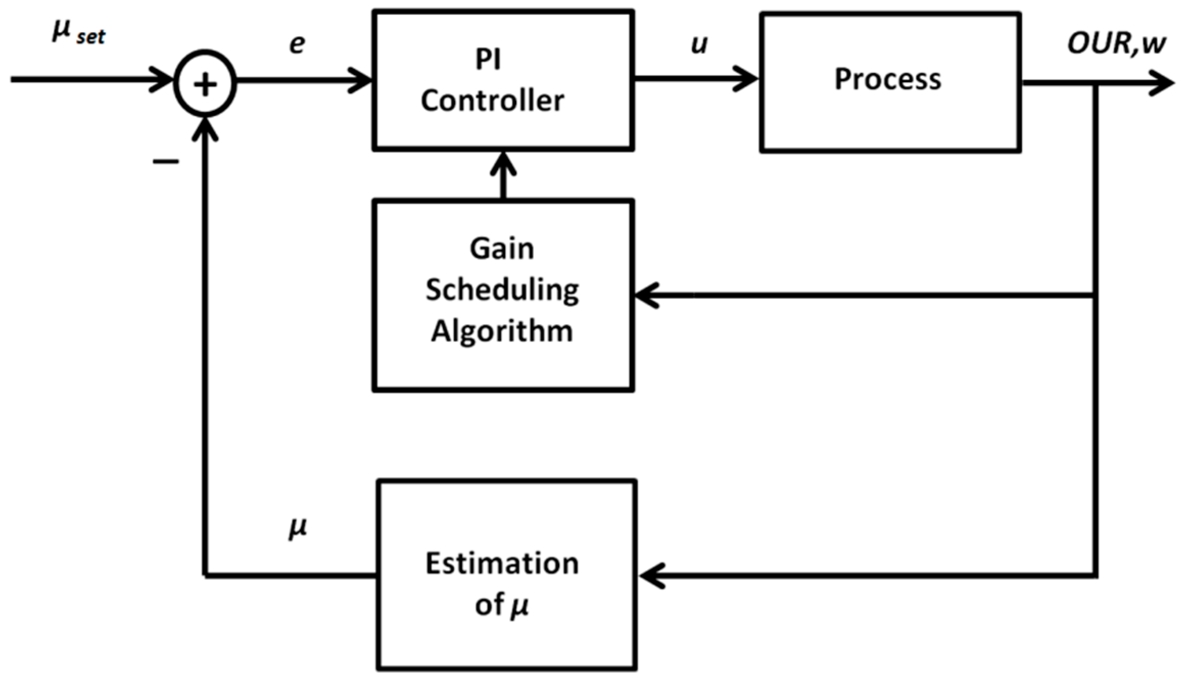
2.2.1. Adaptive PID Control Based on the Gain Scheduling Technique

Because of the nonlinear and non-stationary behavior of the investigated biotechnological processes, application of the ordinary PID control algorithm is limited. Depending on the operating point of the system, the dynamic response (that is defined by varying resultant gain and time constants) of the controlled process may vary, thus requiring corresponding changes of the controller tuning parameters. Such an adaptation of the parameters is required to meet the control quality and stability requirements. As an alternative to the ordinary PID control algorithm, adaptive control techniques may be applied. A promising approach is the gain scheduling technique that implies an application of additional online measurements and construction of the functional relationships used for adaptation of the controller parameters. To identify such relationships, a detailed insight into the dynamic properties of the controlled process is required. For this purpose, a part of Equations (1)–(9) will be transformed to explicit the relationship between the control variable u (substrate feeding rate) and the process variable μ (biomass specific growth rate, SGR). The latter will be controlled in a closed-loop mode. As the SGR is not directly measurable online, one needs to use an auxiliary variable and a state estimator to calculate the signal required for the feedback loop. After analyzing the process model, the oxygen uptake rate OUR was selected as a suitable additional variable, as it adequately reflects the physiologic state of the culture, is well correlated with the biomass growth rate, and can be precisely measured in a bioreactor-scale cultivation process. The structure of the proposed adaptive PID control system is shown in Figure 3.
To investigate how the controller parameters should be adapted online, Equation (2) is linearized at the operating point s*. Taking into account Equations (2), (6) and (9), the following equations are valid at the operating point at steady-state conditions:
d s d t = 0 ,
u = O U R * Y ox Y xs + x * w * ( m m ox Y ox Y xs ) s f s * .
The linearization of Equation (2) at the operating point results in
d ( Δ s ) d t = u w ( Δ s ) + s f s w Δ u .
After transformation of Equation (12), the following first-order differential equation is obtained:
w u d ( Δ s ) d t + ( Δ s ) = s f s u Δ u ,
where the process output is a change of concentration, Δs; and the process input is a change of substrate feeding rate, Δu. The structure of the corresponding process transfer function (in Laplace transform) at the operating point is:
W ( s ) = Δ s ( s ) Δ u ( s ) = K 0 τ s + 1 ,
where the gain coefficient K0 and the time constant τ of the transfer function (14) are as follows:
K 0 = s f s u = ( s f s ) 2 O U R * Y ox Y xs + x * w * ( m m ox Y ox Y xs ) ,
τ = w u = ( s f s ) w * O U R * Y ox Y xs + x * w * ( m m ox Y ox Y xs ) .
The process transfer function (14) has no clearly defined time delay. Hence, for the tuning of the controller parameters, it is not possible to apply the tuning rules involving time delay. Additionally, for a process model of this structure, the derivative part of the PID controller is not able to additionally improve the control quality compared to a control system based on the PI controller. To investigate the functional relationships between the controller’s tuning parameters and the process variables, it is advantageous to write down the internal model control (IMC)-based tuning rules for the PI controller [28], which for the first-order process model are the following:
K C = τ ε K 0 ,
τ i = τ ,
where KC is a proportional gain, τi is an integral time constant, and ε is a tuning parameter (filter time constant). After taking into account Equations (15) and (16) and accepting the assumption that s f s * , the following tuning rules for the investigated process model were obtained:
K C = w * ε s f ,
τ i = s f O U R * / w * Y ox Y xs + x * ( m m ox Y ox Y xs ) .
The transfer function (14) establishes the relationship between the substrate concentration s (state variable) and the substrate feeding rate u (control variable). However, the final aim is to control the specific growth rate µ. For this purpose, it is important to investigate the relationship between the specific growth rate µ and the substrate concentration s. As it can be seen from Equation (9), µ depends on the substrate concentration s and temperature T. The temperature is changed stepwise during the induction and is kept constant within an entire process phase. Over the entire range of possible substrate concentrations, the µ(s) function follows the Haldane-type limitation–inhibition kinetics (see Figure 4a). Nevertheless, the inhibition term may be omitted when investigating the SGR control by means of the limiting substrate feeding, as the substrate concentration during this phase remains low (s = [0, 0.05] (g/kg), see Figure 4b). In this phase, the influence of the inhibition term on the overall µ(s) modeling accuracy is marginal. If the substrate concentrations remain within the range of ~5 × Ks, the inhibition term may be neglected. Despite that the µ(s) function (5) is nonlinear, one can assume that the relationship follows the linear law within this narrow range (i.e., the sensitivity Δµ/Δs may be set to some average value). In such case, the following adaptation rules of the PI controller for the entire control channel u-s-µ can be defined:
K C = w * ε s f ( Δ μ / Δ s ) κ 0 w * ,
τ i = s f O U R * / w * Y ox Y xs + x * ( m m ox Y ox Y xs ) κ 1 O U R * / w * + κ 2 ,
where κ0, κ1 and κ2 are the constants to be identified during the controller tuning procedure. For practical reasons, in the final expression (22), the variable term containing x* in the denominator is substituted by a constant κ2, as the term is significantly smaller than the one including OUR*/w*. This simplification holds even in the second phase of the process, where x* is at the largest. The tuning parameters KC and τi are updated online every time the measured signals of OUR* and w* are received from the process.
It is important to stress that despite the adaptation rules (21) and (22) being based on the OUR and w signals, the adaptive closed-loop control system still needs the feedback signal of the specific growth rate µ (see Figure 3). As this process variable is not directly measured online, an estimator based on the online measurable signals needs to be developed. A logical and straightforward solution is to make use of the OUR signal that is already used for the adaptation of the controller tuning parameters in Equations (21) and (22).
Hence, a relatively simple state estimator, which is based on a numeric integration of the differential Equation (1), was developed and tested. After transforming Equations (9) and (1) into discrete-time form, the following equations of the estimator were obtained:
μ ( t i ) = O U R ( t i ) / w ( t i ) m ox x ( t i 1 ) Y ox x ( t i 1 ) ,
x ( t i ) = x ( t i 1 ) + Δ t i ( μ ( t i ) x ( t i 1 ) Δ w ( t i ) Δ t i x ( t i 1 ) w ( t i ) ) ,
where Δti is the ith sampling time interval.
The estimator makes use of the measured signals of OUR(ti) and w(ti). The initial value of x(t0) is obtained from the off-line measurements at the beginning of the process. During the process, the real-time estimator recursively calculates the online estimates of µ and x. Performance of the estimator in a fed-batch process is presented in Figure 5. In the plots shown, the induction takes place at the 8 h time point, when the SGR is sharply reduced by means of substrate limitation and the temperature drops. Starting from that moment, the process enters the protein production phase.
The results presented in Figure 5 demonstrate the data from a process without closed-loop control of the SGR. In this process, the cell growth was controlled by executing a pre-optimized feeding rate profile. As it can be seen from the plot in Figure 5c, the most intensive fluctuations of the µ estimates are present in the first part of the process. They were caused by a relatively high additive measurement noise in the OUR signal. As the SGR estimates are further used to recursively calculate the biomass concentrations by means of Equation (24), it is also important to compare the biomass estimates against the reference measurements. As it can be seen in Figure 5d, there is no evidence of a systematic drift or significant temporary deviations of the x estimates compared with the reference measurements performed off-line. In the investigated process, MAPE of the biomass concentration estimation did not exceed 2%, whereas standard accuracy of the reference measurements was approximately 5%.
The average values of the model parameters Yox and mox were identified from historic process data collected from multiple runs. Within a series of cultivations, the parameter variation did not exceed 5%. Such variation does not significantly affect the model estimation quality and the µ estimates remain within the acceptable range. To further improve the estimation quality, the estimator may be enhanced by a real-time identification algorithm that makes use of the reference biomass measurements obtained during the process or, alternatively, by using more advanced-state estimation techniques [29,30]. Both the simulation and the real application results have demonstrated that the estimator (23) and (24) is suitable for practical application in the investigated processes. The state estimator was further applied in both investigated adaptive control systems.

2.2.2. Model-Free Adaptive ANN-Based Control

Design of the adaptive PI controller based on the gain scheduling technique revealed that such an approach requires detailed knowledge of the process mathematical model and its dynamic behavior. This is not always the case in industrial practice. Even though the backbone of a fed-batch process model is the set of differential equations (e.g., Equations (1), (2), and (4)) based on mass conservation law, the kinetic expressions (e.g., Equations (5), (6), and (8)) still could be rather different depending on some distinct features of the involved microorganism or its cultivation conditions. This may lead to a different solution regarding the control law or adaptation rule selection. Such detailed understanding of the process may not always be present, posing limitations on the application of the approach detailed in the previous section. Hence, an alternative data-based approach was selected and investigated. Such a control algorithm does not utilize an explicit mathematical model of the process. The structure of such a control system is depicted in Figure 6.
The applied model-free adaptive (MFA) control technique is based on the approach initially introduced by Cheng [31] and was further modified, inter alia, to eliminate the nonlinear transformations in the output layer of the controller. The general architecture of the proposed MFA controller is depicted in Figure 7. The controller is a two-layer feed-forward artificial neural network (ANN) with the time-delayed sequence of the tracking errors in the input layer. The hidden layer of the controller consists of the nodes with nonlinear activation functions φ. The output layer follows the linear law. Additionally, the control algorithm features an error signal that is “bypassed” and added to the resulting controller output. Finally the signal is multiplied by the controller gain KC.
The MFA controller does not require precise knowledge of the controlled process, the control system does not contain an identification mechanism, the controller does not need to be redesigned for a new process and does not require complicated manual tuning, and the closed-loop system stability analysis and criteria are available to guarantee the system stability [31]. The MFA control quality criterion to be minimized is defined as follows:
E ( t ) = 1 2 ( y s e t ( t ) y ( t ) ) 2 = 1 2 e ( t ) 2 ,
where yset(t) is the setpoint, y(t) is the controlled process variable, and e(t) is the tracking error.
The E(t) is minimized by (i) the controller that forces the y(t) to follow the setpoint yset(t) by manipulating the control action u(t); and (ii) the changing of the controller ANN weights w and h (see Figure 7) so that the controller can adapt to the changes in the process dynamics and efficiently reject the process disturbances.
A sigmoidal function is used as the activation function in the neural controller:
φ ( x ) = 1 1 + e x .
The controller output is calculated based on the following equations:
p j ( n ) = i = 0 N w i j ( n ) E i ( n ) ,
q j ( n ) = φ ( p j ( n ) ) ,
o ( n ) = j = 0 N h j ( n ) q j ( n ) ,
v ( t ) = K C ( o ( t ) + e ( t ) ) ,
where n is the nth iteration of the discrete-time control system; pj(n) is the input of the jth activation function in the hidden layer; wij(n) is the ijth weight in the hidden layer; Ei(n) is the ith error signal; qj(n) is the output of the jth activation function in the hidden layer; o(n) is the output of the output layer; hj(n) is the jth weight of the output layer; o(t) is the continuous function of o(n); e(t) is the continuous error signal function; KC is the controller gain coefficient; and v(t) is the continuous function of the controller output (control variable).
The online learning algorithm updates the weights of the MFA controller in the following way:
Δ w i j ( n ) = η K C y ( n ) u ( n ) e ( n ) q j ( n ) ( 1 q j ( n ) ) E i ( n ) k = 0 N h k ( n ) ,
Δ h j ( n ) = η K C y ( n ) u ( n ) e ( n ) q j ( n ) ,
where Δwij(n) is the change of the wij(n) weight in the nth iteration; Δhj(n) is the change of the hj(n) weight in the nth iteration; η is a positive constant of the learning rate; and y ( n ) / u ( n ) is the sensitivity of the process output y(t) with respect to the variations of the process input (control action) u(t).
Through the stability analysis of the MFA control, it was found that, if the controlled process is open-loop stable and controllable, bounding y ( n ) / u ( n ) with a set of nonzero constants can guarantee the system to be bounded-input bounded-output (BIBO) [31]. Therefore, in this study y ( n ) / u ( n ) was replaced by 1. This resulted in the following learning algorithm:
Δ w i j ( n ) = η K C e ( n ) q j ( n ) ( 1 q j ( n ) ) E i ( n ) k = 0 N h k ( n ) ,
Δ h j ( n ) = η K C e ( n ) q j ( n ) .
The MFA control algorithm contains two tuning parameters, η and KC, that need to be adjusted to achieve the best possible control performance.

2.3. Numerical Simulation Techniques

Behavior of the controlled process and performance of the control algorithms were further investigated by means of computer simulations. The model of the process and the control algorithms were programmed in MATLAB (MathWorks, Inc., Natick, MA, USA). To improve the calculation performance, the most time-consuming parts of the code were written in C language and connected with the .m code using a gateway function. The C code was compiled using free MS Windows SDK 7.1 compiler (Microsoft Corporation, Redmond, WA, USA). The dynamic part of the process model was numerically integrated using an ODE solver (C code) based on the fifth-order Cash–Karp Runge–Kutta algorithm with monitoring of local truncation error to ensure accuracy and adjust step size [32].

3. Results

To investigate the behavior of the process and the control system, a typical pattern including several step changes of the SGR and typical disturbances was designed and modeled. An example of the investigated process run is shown in Figure 8. The setpoint of the SGR profile was changed several times (every hour, from 3 till 8 h) to test the control quality in various operation points of the process. These switching points are characterized by a different biomass concentration as well as different SGR setpoints. Additionally, to test the disturbance rejection capabilities of the controller at different loads, temporary malfunctions of the pump performance were simulated at the 7.5 and 9 process hours. The OUR signal was corrupted with additive white Gaussian noise.
Tuning of the adaptive PI controller was performed to minimize the average tracking error (IAE). The tuning was performed using a set of the test runs that covered a wide range of operating conditions and by optimizing the adaptation coefficients κ0, κ1 and κ2. For optimization, an evolutionary computation algorithm [33] was adapted and used. The MFA controller was initially tuned by selecting the parameters η and KC so that the process remained stable in a wide range of the operating conditions. The optimized values of the tuning coefficients are listed in Table 2.
Both investigated control algorithms were tested under various conditions that affected the control quality. During the tests, the variance of the additive white Gaussian noise was varied from 0 to 0.05. An adaptation/learning iteration was performed every time new data were received by the controllers. The discrete-time control algorithms were tested with a feedback signal sampling interval ranging from 1 to 15 s. These values correspond to the realistic intervals used in bioreactor control systems. The control performance results for both controllers, obtained with 0.005 variance and 5 s sampling interval, are depicted in Figure 9. The plots show transient processes that were caused by setpoint changes (Figure 9a,c) and by disturbance (Figure 9b,d). The disturbance was a temporary reduction of the substrate feeding pump performance by 50%. As it can be seen from the plots, both controllers deliver comparable control quality. Calculation of IAE error for each process revealed that the differences between the control quality of the investigated controllers did not exceed 5%–10%. Neither of the two controllers demonstrated a clear advantage. The adaptive PI controller tended to perform better under high SGR conditions, and the MFA controller resulted in lower tracking error when operating under low SGR conditions. In the investigated simulation runs, the average tracking error did not exceed 0.01 (1/h). The temporary overshoots caused by the maximal disturbances stayed within the range of 0.025–0.11 (1/h).
Figure 10a,b depicts the adaptation trajectories of the PI controller parameters KC and τi, respectively. The variation span of the controller gain KC did not exceed 10%, as the parameter is proportional to the culture broth weight that changed moderately during the process. Integration time constant τi follows the changes of the OUR profile and; therefore, reflects the significantly varying dynamics of the process.
Figure 11a,b shows the trajectories of the randomly initialized weights wij and hj of the MFA controller during the learning process. The step-wise changes of the weight values correspond to the SGR changes due to a setpoint change or disturbance, while the continuous drift was caused by slow changes of the related process state variables (i.e., biomass concentration and culture broth weight).
As the MFA controller weights are initialized as random numbers within the interval [−0.5; 0.5], it was important to investigate the influence of the random realization of the weights on the control performance. For this purpose, numerous tests were run with various initial sets of the controller weights, and the control quality was monitored. Figure 12 demonstrates the control performance obtained for 10 test runs. The weights for every run were initialized randomly. However, the results show that the controlled SGR trajectories did not differ significantly. Additionally, the calculated IAE did not show inacceptable variations.
Robustness and control quality of the MFA controller was tested for ANN architectures of various complexity. For the investigated process, the MFA controller with one and two nodes in the hidden layer proved to deliver sufficient tracking quality. The MFA controller with one node in the hidden layer resulted in two weights wij and two weights hj. Further increasing the complexity of the MFA controller did not yield significantly better controller performance.

4. Discussion

The investigated closed-loop control approaches demonstrate clear advantages over the open-loop control systems, which cannot compensate the SGR deviations caused by the process disturbances and equipment malfunctions. The study also revealed that both control systems were stable within the investigated range of the sampling intervals of the feedback signal and the noise levels of the measured signals.
In terms of practical implementation, the proposed adaptive control systems require application of the continuous-flow peristaltic pumps and installation of the off-gas analyzers/flow meters, so that the resulting gas transport delay and time constants of the measuring devices do not exceed the applicable sampling interval of the closed-loop control system.
The obtained results show that, in terms of control performance, both investigated controllers are suitable for biomass specific growth rate control in fed-batch biotechnological processes when using substrate limitation approach and substrate feeding rate manipulation. However, taking into account the efforts for controller design and tuning, including development of the adaptation/learning algorithms, the MFA controller is more attractive for practical applications, especially when only limited knowledge of the process and its mathematical model is available.
The investigated MFA controller also tended to deliver better control quality under low specific growth rate conditions that are prevalent during the recombinant protein production phase. Hence, the MFA control algorithm can be considered as a promising candidate for controlling the specific growth rate in fed-batch recombinant protein production processes. Application of the algorithm can be further extended to SGR control in other bacterial and mammalian cell cultivations that run under substrate limitation conditions.

Author Contributions

Conceptualization, V.G. and R.S.; methodology, V.G. and R.S.; software, V.G.; validation, V.G.; formal analysis, V.G.; investigation, V.G., R.S. and V.V.; resources, V.G.; data curation, V.G.; writing—original draft preparation, V.G.; writing—review and editing, V.G.; visualization, V.G.; supervision, V.G.; project administration, V.G.; funding acquisition, V.G., R.S. and V.V.

Funding

This research was funded by the European Regional Development Fund according to the supported activity “Research Projects Implemented by World-Class Researcher Groups” under the Measure No. 01.2.2-LMT-K-718.

Conflicts of Interest

The authors declare no conflict of interest.

References

  1. Boudreau, M.A.; McMillan, G.K. New Directions in Bioprocess Modelling and Control: Maximizing Process Analytical Technology Benefits; ISA: Durham, NC, USA, 2006; ISBN 978-1-556-17905-1. [Google Scholar]
  2. Dochain, D. Bioprocess Control; ISTE: London, UK, 2008; ISBN 978-0-470-61112-8. [Google Scholar]
  3. Food and Drug Administration. Guidance for Industry. PAT—A Framework for Innovative Pharmaceutical Development, Manufacturing, and Quality Assurance. 2004. Available online: https://www.fda.gov/regulatory-information/search-fda-guidance-documents/pat-framework-innovative-pharmaceutical-development-manufacturing-and-quality-assurance (accessed on 1 October 2019).
  4. Simutis, R.; Lübbert, A. Bioreactor control improves bioprocess performance. Biotechnol. J. 2015, 10, 1115–1130. [Google Scholar] [CrossRef] [PubMed]
  5. Galvanauskas, V.; Simutis, R.; Levišauskas, D.; Urniežius, R. Practical solutions for specific growth rate control systems in industrial bioreactors. Processes 2019, 7, 693. [Google Scholar] [CrossRef]
  6. Schuler, M.M.; Marison, I.W. Real-time monitoring and control of microbial bioprocesses with focus on the specific growth rate: Current state and perspectives. Appl. Microbiol. Biotechnol. 2012, 94, 1469–1482. [Google Scholar] [CrossRef] [PubMed]
  7. Rocha, I.; Veloso, A.; Carneiro, S.; Costa, R.; Ferreira, E. Implementation of a specific rate controller in a fed-batch E. coli fermentation. IFAC Proc. Vol. 2008, 41, 15565–15570. [Google Scholar] [CrossRef]
  8. Puertas, J.; Ruiz, J.; Vega, M.R.; Lorenzo, J.; Caminal, G.; González, G. Influence of specific growth rate over the secretory expression of recombinant potato carboxypeptidase inhibitor in fed-batch cultures of Escherichia coli. Process. Biochem. 2010, 45, 1334–1341. [Google Scholar] [CrossRef]
  9. Lim, H.C.; Shin, H.S. Fed-batch Cultures: Principles and Applications of Semi-Batch Bioreactors; Cambridge Series in Chemical Engineering; Cambridge University Press: Cambridge, UK, 2013; ISBN 978-0-521-51336-4. [Google Scholar] [CrossRef]
  10. Mears, L.; Stocks, S.M.; Sin, G.; Gernaey, K.V. A review of control strategies for manipulating the feed rate in fed-batch fermentation processes. J. Biotechnol. 2017, 245, 34–46. [Google Scholar] [CrossRef]
  11. Lee, J.; Lee, S.Y.; Park, S.; Middelberg, A.P.J. Control of fed-batch fermentations. Biotechnol. Adv. 1999, 17, 29–48. [Google Scholar] [CrossRef]
  12. Åkesson, M.; Hagander, P. A gain-scheduling approach for control of dissolved oxygen in stirred bioreactors. IFAC Proc. Vol. 1999, 32, 7608–7613. [Google Scholar] [CrossRef]
  13. Kuprijanov, A.; Gnoth, S.; Simutis, R.; Lübbert, A. Advanced control of dissolved oxygen concentration in fed batch cultures during recombinant protein production. Appl. Microbiol. Biotechnol. 2009, 82, 221–229. [Google Scholar] [CrossRef]
  14. Gnoth, S.; Kuprijanov, A.; Simutis, R.; Lübbert, A. Simple adaptive pH control in bioreactors using gain-scheduling methods. Appl. Microbiol. Biotechnol. 2009, 85, 955–964. [Google Scholar] [CrossRef]
  15. Levišauskas, D. An algorithm for adaptive control of dissolved oxygen concentration in batch culture. Biotechnol. Tech. 1995, 9, 85–90. [Google Scholar] [CrossRef]
  16. Levišauskas, D.; Simutis, R.; Galvanauskas, V. Adaptive set-point control system for microbial cultivation processes. Nonlinear Anal. Model. Control. 2016, 21, 153–165. [Google Scholar] [CrossRef] [Green Version]
  17. Babuška, R.; Damen, M.R.; Hellinga, C.; Maarleveld, H. Intelligent adaptive control of bioreactors. J. Intell. Manuf. 2003, 14, 255–265. [Google Scholar] [CrossRef]
  18. Smets, I.Y.; Claes, J.E.; November, E.J.; Bastin, G.P.; Impe, J.F. Optimal adaptive control of (bio) chemical reactors: Past, present and future. J. Process. Contr. 2004, 14, 795–805. [Google Scholar] [CrossRef]
  19. Bastin, G.; Impe, J.F. Nonlinear and adaptive control in biotechnology: A tutorial. Eur. J. Contr. 1995, 1, 37–53. [Google Scholar] [CrossRef]
  20. Ginkel, S.Z.; Dooley, T.P.; Suling, W.J.; Barrow, W.W. Identification and cloning of the Mycobacterium avium folA gene, required for dihydrofolate reductase activity. FEMS Microbiol. Lett. 2006, 156, 69–78. [Google Scholar] [CrossRef] [PubMed]
  21. Levišauskas, D.; Galvanauskas, V.; Henrich, S.; Wilhelm, K.; Volk, N.; Lübbert, A. Model-based optimization of viral capsid protein production in fed-batch culture of recombinant Escherichia coli. Bioproc. Biosyst. Eng. 2003, 25, 255–262. [Google Scholar] [CrossRef]
  22. Galvanauskas, V.; Volk, N.; Simutis, R.; Lübbert, A. Design of recombinant protein production processes. Chem. Eng. Comm. 2004, 191, 732–748. [Google Scholar] [CrossRef]
  23. Gasser, B.; Saloheimo, M.; Rinas, U.; Dragosits, M.; Rodríguez-Carmona, E.; Baumann, K.; Villaverde, A. Protein folding and conformational stress in microbial cells producing recombinant proteins: A host comparative overview. Microb. Cell. Fact. 2008, 7, 11. [Google Scholar] [CrossRef]
  24. Gnoth, S.; Jenzsch, M.; Simutis, R.; Lübbert, A. Product formation kinetics in genetically modified E. coli bacteria: Inclusion body formation. Bioproc. Biosyst. Eng. 2007, 31, 41–46. [Google Scholar] [CrossRef]
  25. Gnoth, S.; Simutis, R.; Lübbert, A. Selective expression of the soluble product fraction in Escherichia coli cultures employed in recombinant protein production processes. Appl. Microbiol. Biotechnol. 2010, 87, 2047–2058. [Google Scholar] [CrossRef] [PubMed]
  26. Luedeking, R.; Piret, E.L. A kinetic study of the lactic acid fermentation. Batch process at controlled pH. Biotechnol. Bioeng. 2000, 67, 636–644. [Google Scholar] [CrossRef]
  27. Pirt, S.J. Principles of Microbe and Cell Cultivation; Blackwell Scientific Publications: Oxford, UK, 1985; ISBN 978-0-632-01455-2. [Google Scholar]
  28. Rivera, D.E.; Morari, M.; Skogestad, S. Internal model control: PID controller design. Ind. Eng. Chem. Process. Des. Dev. 1986, 25, 252–265. [Google Scholar] [CrossRef]
  29. Simutis, R.; Lübbert, A. Hybrid approach to state estimation for bioprocess control. Bioengineering 2017, 4, 21. [Google Scholar] [CrossRef] [PubMed]
  30. Urniezius, R.; Survyla, A.; Paulauskas, D.; Bumelis, V.A.; Galvanauskas, V. Generic estimator of biomass concentration for Escherichia coli and Saccharomyces cerevisiae fed-batch cultures based on cumulative oxygen consumption rate. Microb. Cell Factories 2019, in press. [Google Scholar] [CrossRef]
  31. Cheng, G.S. Model Free Adaptive control with CYBOCON. In Techniques for Adaptive Control; VanDoren, V.J., Ed.; Butterworth-Heinemann: Amsterdam, The Netherlands, 2003; pp. 145–202. [Google Scholar]
  32. Press, W.H.; Vetterling, W.T. Numerical Recipes; Cambridge University Press: Cambridge, UK, 2007. [Google Scholar]
  33. Fogel, D.B. Evolutionary Computation toward a New Philosophy of Machine Intelligence; John Wiley & Sons: Hoboken, NJ, USA, 2006. [Google Scholar]
Figure 1. Biomass (solid triangles) and glucose (solid circles) concentrations measured during two fed-batch cultivations (subplots (a) and (b), respectively), along with the corresponding model outputs (solid line and dashed line), determined from Equations (1)–(9).
Processes 07 00810 g001
Figure 2. Specific concentration of viral capsid protein VP1, px (solid squares) obtained from two fed-batch cultivations (subplots (a) and (b), respectively), along with the corresponding model outputs (solid line) and the biomass specific growth rate, μ (dashed line), determined from Equations (1)–(9).
Processes 07 00810 g002
Figure 3. General structure of the adaptive proportional–integral–derivative (PID) control system for specific growth rate control.
Processes 07 00810 g003
Figure 4. µ(s) kinetics (Equation (5)): Possible range of s concentrations in the cultivation medium (a), effective range of s concentrations (b) during µ control by means of substrate limitation.
Processes 07 00810 g004
Figure 5. Performance of the specific growth rate estimator in a fed-batch process: Oxygen uptake rate, OUR (a); culture broth weight, w (b); specific growth rate, µ (c); biomass concentration, x (d) (dashed lines—measured online, solid lines—estimated online, squares—measured off-line).
Processes 07 00810 g005
Figure 6. General structure of the adaptive artificial neural network (ANN)-based control system for specific growth rate control.
Processes 07 00810 g006
Figure 7. Architecture of the ANN-based model-free adaptive (MFA) controller: e(t) is the tracking error; z−1 is the discrete delay function; Ei is the ith error signal; wij is the ijth weight in the hidden layer; pj is the input of the jth activation function in the hidden layer; φ is a sigmoidal activation function; qj is the output of the jth activation function in the hidden layer; hj is the jth weight of the output layer; o(t) is the continuous function of the output; KC is the controller gain coefficient; and v(t) is the continuous function of the controller output.
Processes 07 00810 g007
Figure 8. Specific growth rate (a) and substrate feeding rate (b) trajectories during a test run.
Processes 07 00810 g008
Figure 9. Transient processes of the specific growth rate during a test run: Setpoint change (a) and (c); disturbance rejection (b) and (d); the setpoint (dotted line); adaptive PI-based control (dashed line); ANN-based control (solid line).
Processes 07 00810 g009
Figure 10. Evolution of the PI controller parameters KC (a) and τi (b) during the fed-batch process.
Processes 07 00810 g010
Figure 11. Evolution of the ANN weights wij (a) and hj (b) during the fed-batch process (one node in the hidden layer and one node in the output layer used).
Processes 07 00810 g011
Figure 12. Transient processes of the specific growth rate in a series of 10 test runs (randomly initialized ANN weights): Setpoint change (a) and (c); disturbance rejection (b) and (d); the setpoint (dotted line); ANN-based control (solid line).
Processes 07 00810 g012
Table 1. Values of the model parameters.
Model ParameterValueUnits
Ki93.8 ± 12.7g/kg
K0.0174 ± 0.00121/h
Km751 ± 27U/g
Ks0.01 ± 0.005g/kg
Kµ0.61 ± 0.031/h
m0.0242 ± 0.004g/(gh)
mox0.05 ± 0.0025g/(gh)
sf151g/kg
Tpx1.5 ± 0.1h
Tref37°C
Yox0.7 ± 0.01g/g
Yxs0.46 ± 0.01g/g
α0.0495 ± 0.00251/°C
µmax0.737 ± 0.011/h
Table 2. Optimized values of the tuning parameters.
Model ParameterValueUnits
KC0.4kg
η1.5
κ00.14kg
κ10.008g/kg
κ20.8g/(kg h)

