Modeling and Observer-Based Monitoring of RAFT Homopolymerization Reactions

Abstract

Reversible addition–fragmentation chain–transfer (RAFT) polymerization of methyl methacrylate (MMA) is modeled and monitored using a multi-rate multi-delay observer in this work. First, to fit the RAFT reaction rate coefficients and the initiator efficiency in the model, in situ ${}^1$H nuclear magnetic resonance (NMR) experimental data from small-scale (<2 mL) NMR tube reactions is obtained and a least squares optimization is performed. ${}^1$H NMR and size exclusion chromatography (SEC) experimental data from large-scale (>400 mL) reflux reactions is then used to validate the fitted model. The fitted model accurately predicts the polymer properties of the large-scale reactions with slight discordance at late reaction times. Based on the fitted model, a multi-rate multi-delay observer coupled with an inter-sample predictor and dead time compensator is designed, to account for the asynchronous multi-rate measurements with non-constant delays. The multi-rate multi-delay observer shows perfect convergence after a few sampling times when tested against the fitted model, and is in fair agreement with the real data at late reaction times when implemented based on the experimental measurements.

1. Introduction

Reversible addition–fragmentation chain–transfer (RAFT) polymerization is a living polymerization that is based on free-radical polymerization [1]. Free-radical polymerization reactions are made living by the addition of a RAFT agent, which controls the polymerization via chain equilibration, in which radicals are shared between growing polymer chains. Since RAFT polymerization was first reported by Krstina et al. [2], it has been further investigated by many researchers to show that it works with a wide variety of monomers and RAFT agents [2,3,4,5,6,7,8,9]. RAFT polymerization has been used to create polymers in many fields, including drug delivery [10], electrochemical applications such as fuel cells [11] and batteries [12], and surface modification [13], showing its versatility and applicability.

Key advantages of RAFT polymerization include the synthesis of polymers with narrow polydispersities [1], the ability to form polymers of complex architecture (i.e., block, star), and the ability to work with multiple monomer types—allowing for synthesis of homopolymers and block co-polymers with controlled molecular weights and dispersities. Control of properties such as dispersity and molecular weight is especially important during block copolymer synthesis, in which polymer morphology and micro-phase structure is determined by the polymer block composition [14]. However, no information about these properties is available from online sensors. Offline analysis techniques like ${}^1$H NMR and SEC, which give more insight into the process, require time to analyze samples, and the results are usually obtained after significant delays or even after the whole process is completed. The lack of timely information, which is critical to the progress of polymerization, brings challenges to the quality control of RAFT polymerization. A live model, which accounts for these measurement delays with observers, would be useful for monitoring RAFT polymerization for quality control.

RAFT polymerization was first modeled by Zhang and Ray [15]. They modeled RAFT polymerization of methyl methacrylate in batch, semi-batch, and continuous stirred tank reactors, providing insight into how the mechanism of RAFT polymerization behaved throughout a typical reaction. Many more models have been developed to further explore the fundamentals of RAFT polymerization as more experimental data has become available [16,17,18,19,20,21,22,23]. Few of these models are validated against experimental data at higher monomer conversions, and those that are have few experimental data points above 60% monomer conversion. Additionally, the RAFT agent kinetic rate constants found in these models as fitting parameters are expected to be different for each monomer and RAFT agent pair.

The monitoring of polymerization processes with state estimation techniques based on mathematical models would help target desired polymer compositions and molecular weights during large scale reactions by predicting reaction termination times, and ensuring controlled polymerization by predicting expected dispersities of reactions. However, it is not an easy task to develop the state estimation due to the lack of online measurements and the significant nonlinearity of the systems. There have been a number of studies on state estimation for polymerization applications, with a focus on free radical polymerization, since the early 1980s. The extended Kalman filter (EKF) has been popularly applied to industry with good performance [24,25,26,27,28,29,30,31]. This kind of estimator is designed based on a local linearization approximation and is thereby less effective in the presence of strong system nonlinearities. The state observer, which reconstructs the missing state variables based on the system dynamics with certain feedback terms from the measurement, is an alternative way to design a soft sensor for polymerization processes. For example, Astorga implemented a continuous-discrete observer to an emulsion copolymerization reactor [32]. Appelhaus et al. developed an extended Luenberger observer for a batch polycondensation reactor, in order to get the estimation for concentrations of ethylene glycol and hydroxyl end groups as well as a mass transfer parameter [33]. Several high-gain observers have also been designed for polymerization processes [34,35]. In the observer approach, the convergence properties were mathematically proved under most circumstances, and the computational cost is lowered compared to EKF. Although a significant number of studies have been completed for monitoring different polymerization applications, no state estimation study has been conducted on RAFT polymerizations. Tatiraju and Soroush used a nonlinear open-loop reduced-order observer to estimate the unobservable states in a homopolymerization reactor, and obtained accurate estimation results [36,37]. In our work, a similar idea will be adopted as the basis for the design of a multi-rate multi-delay observer.

One key challenge for the state estimation problem for polymerization is that the measurements are not available at the same rate and usually come with delays. For example, in polymerization processes, the sampling may not be done in a uniform frequency and the measurement information only becomes available after analysis. Therefore, there is a need for the design of a multi-rate multi-delay observer to address this issue. For the multi-rate estimation, the problem has been widely studied based on EKF framework [38]. Moving horizon estimation (MHE) [39,40,41] and other state observer design [37,42,43] have also been investigated. However, most of the EKF and MHE-based methods will not account for the inter-sample dynamic behavior and are incapable of giving estimation for asynchronously sampled measurements. As for the delay effects accompanied with sampling measurements, some observer design approaches were proposed accordingly [44,45,46,47,48,49,50,51], but few of them have been proved stable through a rigorous approach. In some recent works by Ling and Kravaris [52,53,54,55,56,57], a multi-rate multi-delay observer based on a continuous-time design, coupled with inter-sample predictors and dead time compensators, is proposed. Irrespective of perturbations in the sampling schedule, the input-to-output stability property for this observer was first well established for linear systems [53,57], and extended to nonlinear systems with noises [55,56], in the presence of non-uniform and asynchronous measurement with non-constant, arbitrarily large measurement delays, as long as the maximum sampling period does not exceed a certain limit. This observer will be used to estimate the missing information between the sampling measurements for the RAFT polymerization process in the current work.

In this study, small-scale experiments are performed and characterized with in situ ${}^1$H NMR analysis to more accurately monitor RAFT polymerization. Accurate prediction of RAFT specific kinetic rate constants (specifically, $k_{raftf}$, $k_{raftr}$, $k_{raftfR}$ and $k_{raftrR}$) is obtained, allowing for an improved RAFT polymerization model that can be used to monitor larger scale reactions to high monomer conversion values. The improved model is used to test multi-rate, multi-delay observers, which improve predictive modeling of larger scale RAFT reactions allowing for real-time monitoring of reactions and targeted reaction termination times.

2. Model and Observer Design

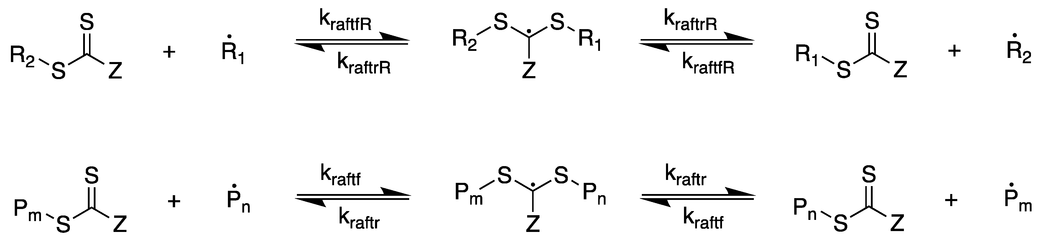
2.1. Modeling RAFT Polymerization—Improving the Model by Zhang and Ray

The RAFT polymerization model used in this work is based on a model presented by Zhang and Ray [15]. This subsection will provide a brief review of their model as well as the specific changes and additions made to their model to help the reader follow subsequent sections of this paper.

RAFT polymerization is modeled by including standard free radical polymerization kinetics (i.e., initiation, propagation, chain transfer and termination) with the RAFT reaction steps in the presence of a RAFT agent. The RAFT reactions are shown in Scheme 1. These RAFT steps create three dormant polymer populations based on the state of the RAFT agent end group. In total, five polymer populations exist within the model: growing polymer chains, dead polymer chains and three types of dormant polymer chains. To simplify the model, these populations are modeled using moments, for which the mathematical definitions are given in

Table 1. Polymer moment definitions.

Chain Type	Moment Definition
Growing Polymer	${\mu }_i={\sum }_{n=1}^{\infty }{n}^i\left[P_n\right]$
Dormant Polymer Type 1	${\nu }_i={\sum }_{n=1}^{\infty }{n}^i\left[P_{n}AR\right]$
Dormant Polymer Type 2	${\xi }_i={\sum }_{n=1}^{\infty }{n}^i\left[P_{n}A\right]$
Dormant Polymer Type 3	${\zeta }_{ij}={\sum }_{n=1}^{\infty }{\sum }_{m=1}^{\infty }{n}^i{m}^i\left[P_{n}A{P}_m\right]$
Dead Polymer	${\lambda }_i={\sum }_{n=1}^{\infty }{n}^i\left[D_n\right]$

. The terms brackets are as follows: [P${}_n$], concentration of growing polymer chain of degree of polymerization n; [P${}_n$AR], concentration of RAFT agent bonded to a primary radical and a polymer chain of degree of polymerization n; [P${}_n$A], concentration of RAFT agent bonded to a polymer chain of degree of polymerization n; [P${}_n$AP${}_m$], concentration of RAFT agent bonded to two polymer chains of degree of polymerization n and m; and [D${}_n$], concentration of dead polymer chains of degree of polymerization n. When using polymer moments, it is not possible to apply different kinetic rate constants based on polymer chain length, and we must make the assumption that the kinetic rate constants are independent of polymer chain length. This assumption, although it may introduce some error, is made out of necessity for model simplicity.

Using these polymer moment definitions and the monomer concentration ($C_M$), the monomer conversion ($X_p$), number average degree of polymerization ($D{P}_n$), weight average degree of polymerization ($D{P}_w$) and dispersity (Đ) can be calculated as shown in Equation (1):

$$\begin{array}{cc}\hfill & X_p={\displaystyle \frac{{\mu }_1+{\nu }_1+{\xi }_1+{\lambda }_1+{\zeta }_{10}}{{\mu }_1+{\nu }_1+{\xi }_1+{\lambda }_1+{\zeta }_{10}+C_M}},\hfill \\ \hfill & D{P}_n={\displaystyle \frac{{\mu }_1+{\nu }_1+{\xi }_1+{\zeta }_{10}+{\lambda }_1}{{\mu }_0+{\nu }_0+{\xi }_0+0.5{\zeta }_{00}+{\lambda }_0}},\hfill \\ \hfill & D{P}_w={\displaystyle \frac{{\mu }_2+{\nu }_2+{\xi }_2+{\zeta }_{20}+0.5{\zeta }_{11}+{\lambda }_2}{{\mu }_1+{\nu }_1+{\xi }_1+{\zeta }_{10}+{\lambda }_1}},\hfill \\ \hfill & Đ={\displaystyle \frac{D{P}_w}{D{P}_n}}.\hfill \end{array}$$

(1)

Using the kinetic scheme from Zhang and Ray and Scheme 1, the 23 balance equations given in Equation (2) are used to represent each of the species in the model. The definitions for the state variables are listed in

Table 2. State variables.

Variables	Description
${\mu }_0$	Growing polymer chain zeroth moment
${\mu }_1$	Growing polymer chain first moment
${\mu }_2$	Growing polymer chain second moment
${\nu }_0$	Dormant polymer chain type 1 zeroth moment
${\nu }_1$	Dormant polymer chain type 1 first moment
${\nu }_2$	Dormant polymer chain type 1 second moment
${\xi }_0$	Dormant polymer chain type 2 zeroth moment
${\xi }_1$	Dormant polymer chain type 2 first moment
${\xi }_2$	Dormant polymer chain type 2 second moment
${\zeta }_{00}$	Dormant polymer chain type 3 zeroth moment
${\zeta }_{10}$	Dormant polymer chain type 3 first moment
${\zeta }_{20}$	Dormant polymer chain type 3 second moment part one
${\zeta }_{11}$	Dormant polymer chain type 3 second moment part two
${\lambda }_0$	Dead polymer chain zeroth moment
${\lambda }_1$	Dead polymer chain first moment
${\lambda }_2$	Dead polymer chain second moment
$C_R$	Concentration of primary radicals
$C_{AR}$	Concentration of RAFT agent
$C_{RAR}$	Concentration of primary intermediate
$C_I$	Concentration of initiator
$C_M$	Concentration of monomer
$C_S$	Concentration of solvent
$C_{CTA}$	Concentration of chain transfer agent

, and the definitions and values for the reaction rate constants are given in

Table 3. Reaction rate constant definitions.

Reaction Rate Constant	Definition	Equation/Value	Units	Reference
$k_d$	Initiator formation	$1.0533\times {10}^{15}{e}^{\frac{-30704}{RT}}$	s${}^{-1}$	[62]
$k_p$	Live chain propagation	${10}^{6.427}{e}^{\frac{-5344}{RT}}$	L mol${}^{-1}$ s${}^{-1}$	[59]
$k_{trM}$	Radical transfer to monomer	$k_p\times {10}^{-5}$	L mol${}^{-1}$ s${}^{-1}$	[63]
$k_{trS}$	Radical transfer to solvent	0, assumed negligible	L mol${}^{-1}$ s${}^{-1}$
$k_{trCTA}$	Radical transfer to CTA	0, assumed negligible	L mol${}^{-1}$ s${}^{-1}$
$k_t$	Termination	${10}^{9.586}{e}^{\frac{-3106}{RT}}$	L mol${}^{-1}$ s${}^{-1}$	[58]
$k_{raftf}$	Forward RAFT main equilibrium	Unknown	L mol${}^{-1}$ s${}^{-1}$
$k_{raftr}$	Reverse RAFT main equilibrium	Unknown	s${}^{-1}$
$k_{raftfR}$	Forward RAFT pre-equilibrium	Unknown	L mol${}^{-1}$ s${}^{-1}$
$k_{raftrR}$	Reverse RAFT pre-equilibrium	Unknown	s${}^{-1}$
f	Initiator efficiency	Unknown

.

This model differs from the Zhang and Ray model in two ways: first, in the way termination is modeled, and second, in the rate constants. In the Zhang and Ray model, termination is modeled accounting for both combination and disproportionation reactions. In this model, termination is modeled accounting for just one general termination reaction based on more recent work in the literature [58]. With this change in how termination reactions are modeled, the corresponding rate constants are also changed. In the Zhang and Ray model, $k_{tc}$ and $k_{td}$ are used to represent the rates for combination and disproportionation reactions, respectively. In this work, a single termination reaction rate constant $k_t$ is used instead to represent all termination reactions. Additionally, the propagation rate constant has been updated from the Zhang and Ray model based on a more recent work in the literature [59]. Finally, two additional kinetic rate constants for the RAFT agent pre-equilibrium reactions are included ($k_{raftfR}$ and $k_{raftrR}$) based on literature [23,60,61] showing a difference for reactions between the RAFT agent and primary radicals when compared to reactions between the RAFT agent and growing polymer chains.

Most of the reaction rate constants are based on free radical polymerization. The exceptions to this are k${}_{trCTA}$, k${}_{raftf}$, k${}_{raftr}$, k${}_{raftfR}$ and k${}_{raftrR}$. These five reaction rate constants are dependent on the choice of RAFT agent used, and are expected to change for each RAFT agent. In this model, the effect of chain transfer to CTA is considered negligible and $k_{trCTA}$ is set to zero:

$$\begin{array}{cc}{\displaystyle \frac{d{\mu }_0}{dt}}=\hfill & k_p{C}_R{C}_M+k_{trm}{\mu }_0{C}_M-k_t(C_R+{\mu }_0){\mu }_0-k_{trm}{\mu }_0{C}_M-k_{trs}{\mu }_0{C}_S\hfill \\ & -k_{trCTA}{\mu }_0{C}_{CTA}-k_{raftf}{\mu }_0(C_{AR}+{\xi }_0)+k_{raftr}({\nu }_0+{\zeta }_{00}),\hfill \\ {\displaystyle \frac{d{\mu }_1}{dt}}=\hfill & k_p{C}_R{C}_M+k_{trm}{\mu }_0{C}_M+k_p{C}_M{\mu }_0-k_t(C_R+{\mu }_0){\mu }_1-k_{trm}{\mu }_1{C}_M-k_{trs}{\mu }_1{C}_S\hfill \\ & -k_{trCTA}{\mu }_1{C}_{CTA}-k_{raftf}{\mu }_1(C_{AR}+{\xi }_0)+k_{raftr}({\nu }_1+{\zeta }_{10}),\hfill \\ {\displaystyle \frac{d{\mu }_2}{dt}}=\hfill & k_p{C}_R{C}_M+k_p{C}_M({\mu }_0+2{\mu }_1)-k_t(C_R+{\mu }_0){\mu }_2-k_{trm}{\mu }_2{C}_M-k_{trs}{\mu }_2{C}_S\hfill \\ & k_{trCTA}{\mu }_2{C}_{CTA}-k_{raftf}{\mu }_2(C_{AR}+{\xi }_0)+k_{raftr}({\nu }_2+{\zeta }_{20}),\hfill \\ {\displaystyle \frac{d{\nu }_0}{dt}}=\hfill & k_{raftf}{\mu }_0{C}_{AR}+k_{raftfR}{C}_R{\xi }_0-k_{raftr}{\nu }_0-k_{raftrR}{\nu }_0,\hfill \\ {\displaystyle \frac{d{\nu }_1}{dt}}=\hfill & k_{raftf}{\mu }_1{C}_{AR}+k_{raftfR}{C}_R{\xi }_1-k_{raftr}{\nu }_1-k_{raftrR}{\nu }_1,\hfill \\ {\displaystyle \frac{d{\nu }_2}{dt}}=\hfill & k_{raftf}{\mu }_2{C}_{AR}+k_{raftfR}{C}_R{\xi }_2-k_{raftr}{\nu }_2-k_{raftrR}{\nu }_2,\hfill \\ {\displaystyle \frac{d{\xi }_0}{dt}}=\hfill & -k_{raftf}{\mu }_0{\xi }_0-k_{raftfR}{C}_R{\xi }_0+k_{raftr}{\zeta }_{00}+k_{raftrR}{\nu }_0,\hfill \\ {\displaystyle \frac{d{\xi }_1}{dt}}=\hfill & -k_{raftf}{\mu }_0{\xi }_1-k_{raftfR}{C}_R{\xi }_1+k_{raftr}{\zeta }_{10}+k_{raftrR}{\nu }_1,\hfill \\ {\displaystyle \frac{d{\xi }_2}{dt}}=\hfill & -k_{raftf}{\mu }_0{\xi }_2-k_{raftfR}{C}_R{\xi }_2+k_{raftr}{\zeta }_{20}+k_{raftrR}{\nu }_2,\hfill \\ {\displaystyle \frac{d{\zeta }_{00}}{dt}}=\hfill & 2k_{raftf}{\mu }_0{\xi }_0-2k_{raftr}{\zeta }_{00},\hfill \\ {\displaystyle \frac{d{\zeta }_{10}}{dt}}=\hfill & k_{raftf}({\mu }_1{\xi }_0+{\mu }_0{\xi }_1)-2k_{raftr}{\zeta }_{10},\hfill \\ {\displaystyle \frac{d{\zeta }_{20}}{dt}}=\hfill & k_{raftf}({\mu }_2{\xi }_0+{\mu }_0{\xi }_2)-2k_{raftr}{\zeta }_{20},\hfill \\ {\displaystyle \frac{d{\zeta }_{11}}{dt}}=\hfill & 2k_{raftf}{\mu }_1{\xi }_1-2k_{raftr}{\zeta }_{11},\hfill \\ {\displaystyle \frac{d{\lambda }_0}{dt}}=\hfill & k_t(C_R+{\mu }_0){\mu }_0+k_{trm}{\mu }_0{C}_M+k_{trs}{\mu }_0{C}_S+k_{trCTA}{\mu }_0{C}_{CTA},\hfill \\ {\displaystyle \frac{d{\lambda }_1}{dt}}=\hfill & k_t(C_R+{\mu }_0){\mu }_1+k_{trm}{\mu }_1{C}_M+k_{trs}{\mu }_1{C}_S+k_{trCTA}{\mu }_1{C}_{CTA},\hfill \\ {\displaystyle \frac{d{\lambda }_2}{dt}}=\hfill & k_t(C_R+{\mu }_0){\mu }_2+k_{trm}{\mu }_2{C}_M+k_{trs}{\mu }_2{C}_S+k_{trCTA}{\mu }_2{C}_{CTA},\hfill \\ {\displaystyle \frac{d{C}_R}{dt}}=\hfill & 2f{k}_d{C}_I-k_p{C}_R{C}_M-k_t{C}_R(C_R+{\mu }_0)+k_{trs}{\mu }_0{C}_S+k_{trCTA}{\mu }_0{C}_{CTA}\hfill \\ & -k_{raftfR}{C}_R(C_{AR}+{\xi }_0)+k_{raftrR}(2C_{RAR}+{\nu }_0),\hfill \\ {\displaystyle \frac{d{C}_{AR}}{dt}}=\hfill & -k_{raftf}{C}_{AR}{\mu }_0-k_{raftfR}{C}_{AR}{C}_R+k_{raftr}{\nu }_0+2k_{raftrR}{C}_{RAR},\hfill \\ {\displaystyle \frac{d{C}_{RAR}}{dt}}=\hfill & k_{raftfR}{C}_R{C}_{AR}-2k_{raftrR}{C}_{RAR},\hfill \\ {\displaystyle \frac{d{C}_I}{dt}}=\hfill & -k_d{C}_I,\hfill \\ {\displaystyle \frac{d{C}_M}{dt}}=\hfill & -k_p{C}_M(C_R+{\mu }_0)-k_{trm}{\mu }_0{C}_M,\hfill \\ {\displaystyle \frac{d{C}_S}{dt}}=\hfill & -k_{trs}{\mu }_0{C}_S,\hfill \\ {\displaystyle \frac{d{C}_{CTA}}{dt}}=\hfill & -k_{trCTA}{\mu }_0{C}_{CTA}.\hfill \end{array}$$

(2)

Methyl methacrylate is known for undergoing the Trommsdorff–Norrish effect (i.e., the gel effect) during polymerization, in which the propagation rate accelerates, and the termination rate decelerates, at high viscosities as growing polymer chains entangle. This effect is included in the model by Zhang and Ray, and was considered in this work. In this work, high solvent to monomer ratios dilute the polymer concentration and prevent the viscosity from increasing high enough to induce the Trommsdorff–Norrish effect, and therefore this effect was not observed.

The large-scale reaction experiments in this work are performed under reflux and do not occur at a constant temperature. As monomer is consumed, the composition, and therefore the bubble point of the volatile components in the reactor change. Temperature of the reactor for large-scale experiments is estimated by calculating the bubble point of a binary mixture based on the volatile components of the reacting mixture (i.e., the solvent and the monomer). Data for the bubble point temperature of the binary mixture was calculated using UNIFAQ in ASPEN, and a polynomial fit was applied to the data and the corresponding equation is shown in Equation (3), where $x_{THF}$ denotes the mole fraction composition of tetrahydrofuran (THF) in the reacting mixture. This fit was used within the model to calculate reaction temperature as a function of reacting mixture composition for the large-scale experiments:

$$T=9.4893x_{THF}^3-4.032x_{THF}^2-39.482x_{THF}+100.13.$$

(3)

The RAFT polymerization model includes the following assumptions. The reactions are performed under ideal mixing. Reactions involving polymers and their corresponding kinetic rate constants are independent of polymer chain length, allowing for polymer moments to be used. All primary radicals are treated as identical, regardless of the reactions leading to their formation (i.e., a primary radical formed from initiator decomposition is identical to a primary radical from chain transfer reactions). Kinetic rate constants $k_{raftf}$, $k_{raftr}$, $k_{raftfR}$ and $k_{raftrR}$ are not dependent on reaction temperature.

2.2. Observer Design

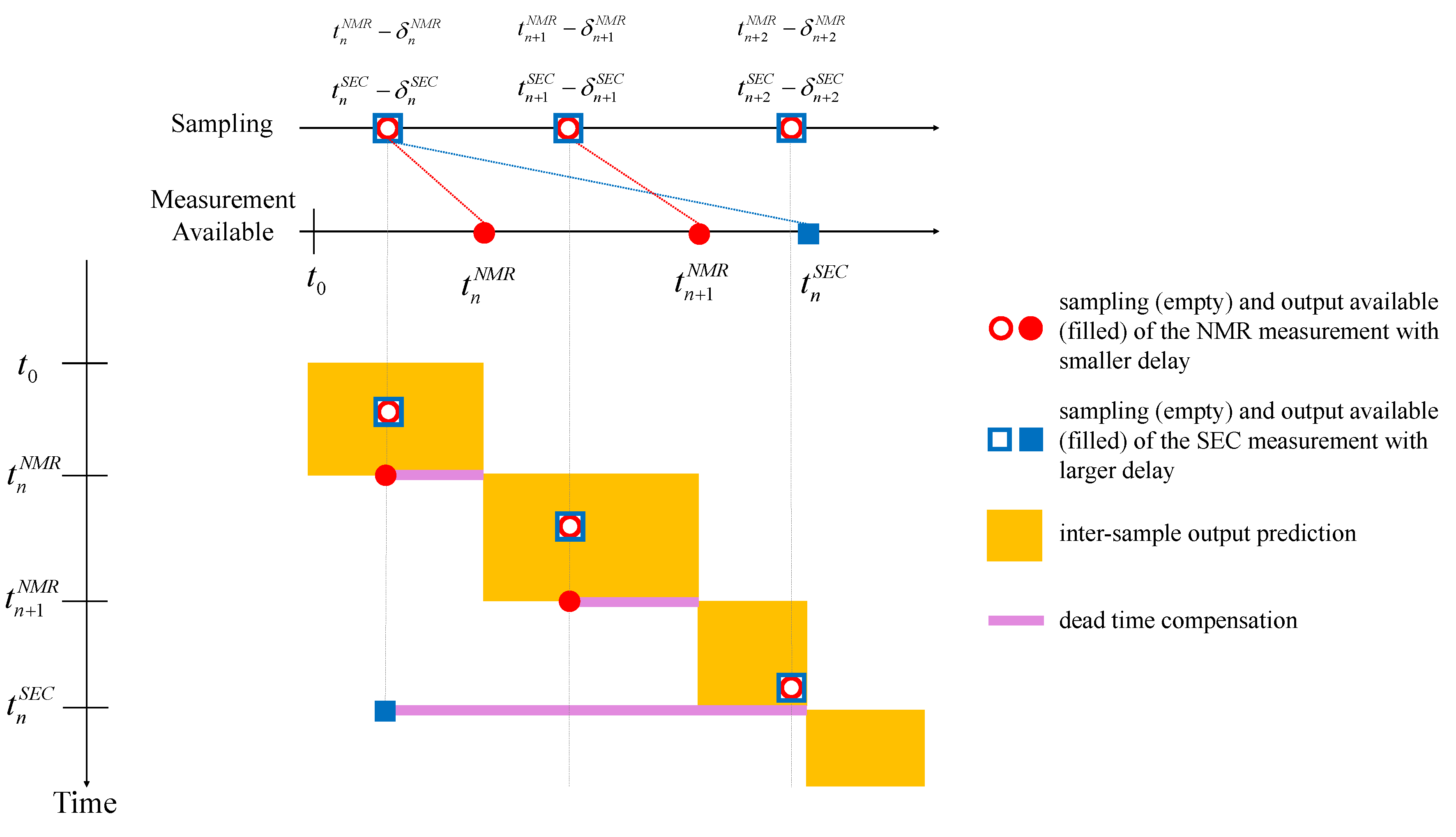
2.2.1. Multi-Rate Multi-Delay Observer—Background

This part gives the basic background for the design method for the multi-rate multi-delay observer used in this work. The state estimation problem for the RAFT polymerization process in the current work will be a special case of the observer presented in this section.

The starting point for the design of the multi-rate multi-delay observer will be a continuous time observer. A reduced order observer that simulates a subsystem driven by the measurements can be built following Soroush [64]. In the following part, the particular observer driven by the measurement is introduced.

For simplicity, consider a continuous system with a part of the state vector to be directly measured. Note that a measurement variable could always be included as a state variable through appropriate coordinate transformation:

$$\begin{array}{cc}\hfill & {\dot{x}}_R(t)=f_R(x_R(t),x_M(t)),\hfill \end{array}$$

(4a)

$$\begin{array}{cc}\hfill & {\dot{x}}_M(t)=f_M(x_R(t),x_M(t)),\hfill \end{array}$$

(4b)

$$\begin{array}{cc}\hfill & y(t)=x_M(t),\hfill \end{array}$$

(4c)

where $x_R\in {\mathbb{R}}^{n-m}$ and $x_M\in {\mathbb{R}}^m$ are the unmeasured and measured state vectors; y is the continuous output. It is assumed that the unmeasured subsystem (4a) is locally asymptotically stable.

A reduced order observer that is driven by the measurable outputs is of the form

$${\dot{\widehat{x}}}_R(t)=f_R({\widehat{x}}_R(t),y(t)),$$

(5)

where ${\widehat{x}}_R\in {\mathbb{R}}^{n-m}$ is the vector of estimated states that guarantee the estimation error $e(t)={\widehat{x}}_R(t)-x_R$ converges to 0 as $t\to \infty$ [64]. This reduced order observer is based on a different philosophy than the traditional closed-loop observers that involve a correction term multiplied by an observer gain. However, it still incorporates the feedback effect in the sense that it uses the measurement to drive the simulation; and the stability of system dynamics would imply the stability of the observer error dynamics.

When the sampling is performed at a slow rate with asynchronous intervals, the missing inter-sample information needs to be accurately predicted by a multi-rate observer. Now, consider the dynamic system (4a) and (4b) with multi-rate slow-sampled measurements

$$\begin{array}{cc}\hfill & {\dot{x}}_R(t)=f_R(x_R(t),x_M(t)),\hfill \\ \hfill & {\dot{x}}_M(t)=f_M(x_R(t),x_M(t)),\hfill \\ \hfill & y^i(t_j^i)=x_M^i(t_j^i),j\in {\mathbb{Z}}_{+},i=1,2,\dots ,m,\hfill \end{array}$$

(6)

where $t_j^i$ denotes the j-th sample time for the i-th measured component of $x_M$, at some sequence of time instants $S={\left\{t_k\right\}}_{k=0}^{\infty }$. The intervals between each sampling time are not necessarily uniform.

A multi-rate observer is designed based on a continuous-time observer, coupled with inter-sample predictors to handle the inter-sample behavior. For the predictor, the dynamic system (6) is simulated to obtain a prediction for the missing output information in between two consecutive measurements. This prediction will then be given to the continuous-time observer (5) functioning as the continuous outputs. For $t\in [t_k^{+},t_{k+1}]$, the multi-rate sampled-data observer for the multi-rate system (6) is [56]:

$$\begin{array}{cccc}\hfill & {\dot{\widehat{x}}}_R(t)=f_R({\dot{\widehat{x}}}_R(t),w(t))\hfill & \hfill & t\in [t_k,t_{k+1}),\hfill \\ \hfill & \dot{w}(t)=f_M({\widehat{x}}_R(t),w(t)),\hfill & \hfill & t\in [t_k,t_{k+1}),\hfill \\ \hfill & w^i(t_{k+1})=y^i(t_{k+1}),\hfill \end{array}$$

(7)

where $w\in {\mathbb{R}}^m$ is the predicted output. The predictors will give continuous estimates of the sampled outputs between two sampling times, but note that these two sampling times $t_k$, $t_{k+1}$ are not necessarily from the same output. The i-th component $w^i(t)$ will be reset to $y^i(t_{k+1})$ once the new measurement obtained, and the other predictor states will not change until the corresponding measurements become available.

Now, consider a system with possible delays in the multi-rate sampled measurement $y^i(t_j^i)$

$$\begin{array}{cc}\hfill & {\dot{x}}_R(t)=f_R(x_R(t),x_M(t)),\hfill \\ \hfill & {\dot{x}}_M(t)=f_M(x_R(t),x_M(t)),\hfill \\ \hfill & y^i(t_j^i)=x_M^i(t_j^i-{\delta }_j^i),j\in {\mathbb{Z}}_{+},i=1,2,\dots ,m,\hfill \end{array}$$

(8)

where $t_j^i$ is the time when j-th measurement of $x_M^i$ is obtained after certain delay ${\delta }_j^i⩾0$. That is to say, the measurement $y^i(t_j^i)$ arrived at $t_j^i$ reflects the value of $x_M^i$ at time $t_j^i-{\delta }_j^i$.

The proposed observer for the system (6) with multiple measurement delays is based on the multi-rate observer design (7) combined with dead time compensation. When the sampled measurement arrives at $t_j^i$ after a delay ${\delta }_j^i$, a dead time compensator would be initiated to recalculate the past estimates for $t\in [t_j^i-{\delta }_j^i,t_j^i]$ with the following observer design [55]:

$$\begin{array}{cc}\hfill & {\dot{\widehat{x}}}_R(t)=f_R({\dot{\widehat{x}}}_R(t),w(t)),\hfill \end{array}$$

(9a)

$$\begin{array}{cc}\hfill & \dot{w}(t)=f_M({\widehat{x}}_R(t),w(t)),\hfill \end{array}$$

(9b)

$$\begin{array}{cc}\hfill & w^i(t_j^i-{\delta }_j^i)=y^i(t_j^i),\hfill \end{array}$$

(9c)

$$\begin{array}{cc}\hfill & w^{i^{\prime }}(t_{j^{\prime }}^{i^{\prime }}-{\delta }_{j^{\prime }}^{i^{\prime }})=y^{i^{\prime }}(t_{j^{\prime }}^{i^{\prime }}),\forall t_{j^{\prime }}^{i^{\prime }},(t_{j^{\prime }}^{i^{\prime }}-{\delta }_{j^{\prime }}^{i^{\prime }})\in [t_j^i-{\delta }_j^i,t_j^i),\hfill \end{array}$$

(9d)

where $w\in {\mathbb{R}}^m$ denotes the corrected state prediction that generates the past estimates for $x_M(t)$. Equation (9c) formulates the reinitialization of the i-th dead time compensator for $x_M^i(t)$ by using the delayed measurement $y^i(t_j^i)$ corresponding to the sampling time $t_j^i-{\delta }_j^i$. The other measurement $y^{i^{\prime }}(t_{j^{\prime }}^{i^{\prime }})$ that is sampled between $t_j^i-{\delta }_j^i$ and $t_j^i$ can be used to reset other corrected state prediction $w^{i^{\prime }}(t)$ at their respective sampling times, as is represented by Equation (9d).

After the dead time compensation has updated the past estimates, the inter-sample prediction will be applied for the missing points between two measurements for $t\in [t_j^i,t_{j^{\prime }}^{i^{\prime }}]$ in the same spirit as the delay-free multi-rate observer (7). If a measurement is available at $t_j^i$ without any delay, then no dead time compensation is needed and the inter-sample prediction runs immediately after reset. A detailed explanation for the estimation process will be given in the following part based on the RAFT polymerization process that is studied in this paper.

2.2.2. Prediction of RAFT Polymerization

Throughout the polymerization, it is important to keep track of monomer conversion ($X_p$), degree of polymerization ($D{P}_n$), and dispersity (Đ) of the polymer formed in the reacting mixture. Monomer conversion shows the reaction is proceeding, and is used to gauge how quickly polymerization occurs. Degree of polymerization is used to target the reaction end point when a desired degree of polymerization is reached. Dispersity is used to gauge the control of the RAFT agent on the polymerization; high dispersities indicate loss of control of the polymerization.

${}^1$H NMR and SEC are used to characterize these properties from the reaction mixture aliquots. However, this data is not available in real time. Data from these analysis techniques become available only after analysis, and the time to perform analysis for each technique differs. In general, ${}^1$H NMR provides monomer conversion ($X_p$) data after a typical delay of approximately 30 min. SEC provides molecular weight data ($M_n$, $M_w$), degree of polymerization data ($DP$), dispersities (Đ), and monomer conversion data ($X_p$) after a typical delay of 4 h. The delays for each technique are inherent to proper sample preparation and analysis procedure for each technique. As a result, reaction data for updating the observer comes with a multi-rate, multi-delay nature.

Note that the concerned measured variables $X_p$, $D{P}_n$ and Đ are not part of the state variables. However, through a coordinate transformation via (1), we can introduce them as three state variables into the dynamic system (2) and substitute three existing states. The RAFT process can be described in the form of Equation (8) with $x_M={\left[X_{p}D{P}_nĐ\right]}^T$ and $x_R$ to be a column vector with 20 remaining state variables out of the 23 variables listed in Table 2. The measurement for the problem could be formulated as

$$\begin{array}{cc}\hfill & y^1(t_j^{NMR})=X_p(t_j^{NMR}-{\delta }_j^{NMR}),\hfill \\ \hfill & y^2(t_{j^{\prime }}^{SEC})=D{P}_n(t_{j^{\prime }}^{SEC}-{\delta }_{j^{\prime }}^{SEC}),j,j^{\prime }\in {\mathbb{Z}}_{+},\hfill \\ \hfill & y^3(t_{j^{\prime }}^{SEC})=Đ(t_{j^{\prime }}^{SEC}-{\delta }_{j^{\prime }}^{SEC}).\hfill \end{array}$$

(10)

As these measurements are sampled with delay, no timely information is available in between measurements. Using observers to monitor the polymerization allows for an estimation of the missing information between each measurement, and thus provides an accurate estimation near the end point of the reaction to guide the operation of processes. Therefore, in this case, instead of the unmeasured states $x_R$, the accurate estimation for $x_M$ is expected from the observer through:

$${\widehat{x}}_M(t)=w(t),$$

(11)

where $w(t)$ is calculated from both the dead time compensator (Section 2.2.1) and the inter-sample predictor (7).

Figure 1 depicts the two-step estimation process from time $t_0$. We will use the workflow after the n-th sample is taken, to demonstrate how the multi-rate multi-delay observer works. As a first step, when the delayed ${}^1$H NMR measurement (which gives $X_p$) for the n-th sample becomes available at $t_n^{NMR}$, the dead time compensation is triggered. Past estimation is generated by integrating the observer and compensator equations for the time range [$t_n^{NMR}-{\delta }_n^{NMR}$, $t_n^{NMR}$]. In this compensator, the new value for $X_p$ is used as a delay-free measurement to reset the corresponding compensator $w^1$. The compensator consequently updates the estimation for all states at $t_n^{NMR}$, the ending time of compensation. This step makes use of the available measurements in the delay-free observer, in the same order as they are sampled. As a second step, the updated estimates are used as the initial condition for the observer coupled with inter-sample output predictors (7) at $t_n^{NMR}$. In addition, this multi-rate multi-delay observer now works like a delay-free multi-rate observer with no delayed measurement, until the next measurement from SEC becomes available at $t_{n+1}^{NMR}$.

Note that the proposed multi-rate multi-delay observer is based on the continuous reduced-order observer (5). It has been proved that, as long as the maximum sampling period satisfies a certain limit, the stability of error dynamics for the continuous observer of (5) implies the validity of the multi-rate multi-delay observer [56]. However, as the continuous observer of (5) does not have a feedback correction term led by an observer gain, the rate of error dynamics is not adjustable.

3. Experimental Methods and Results

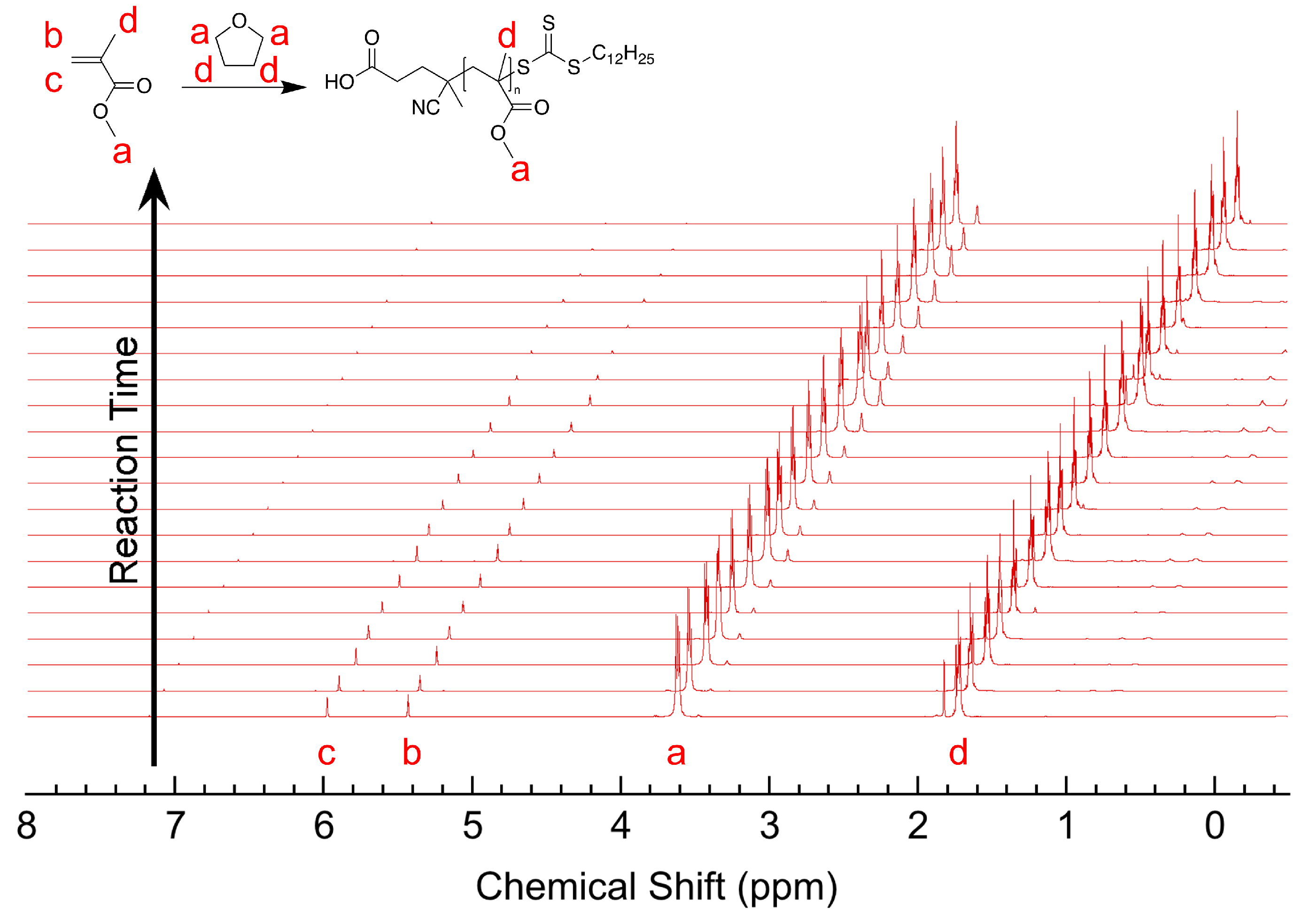
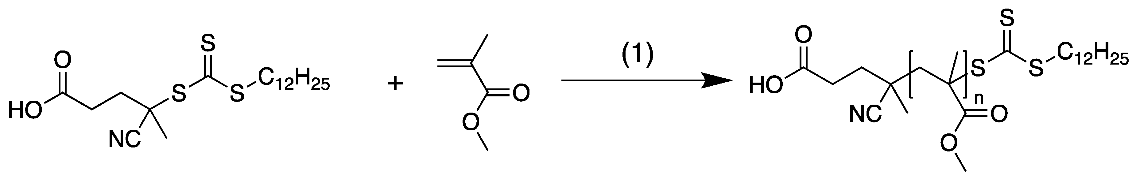
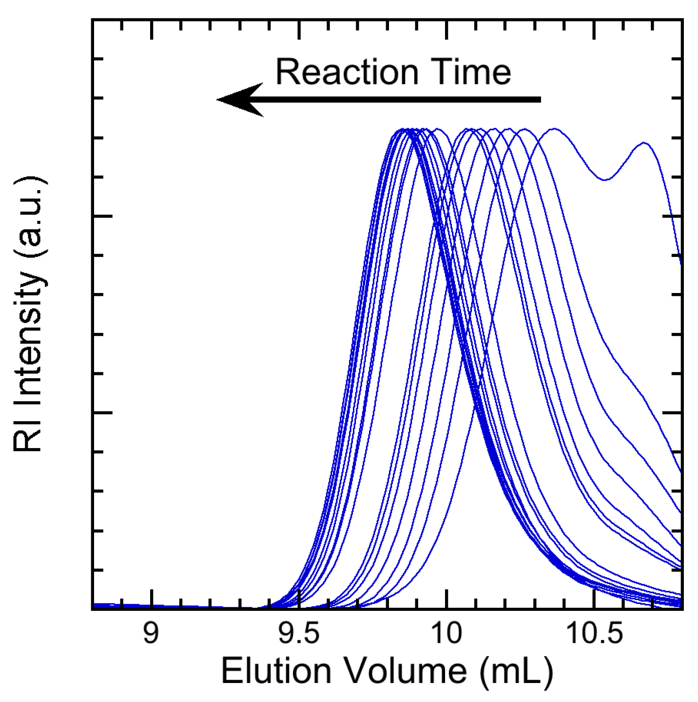
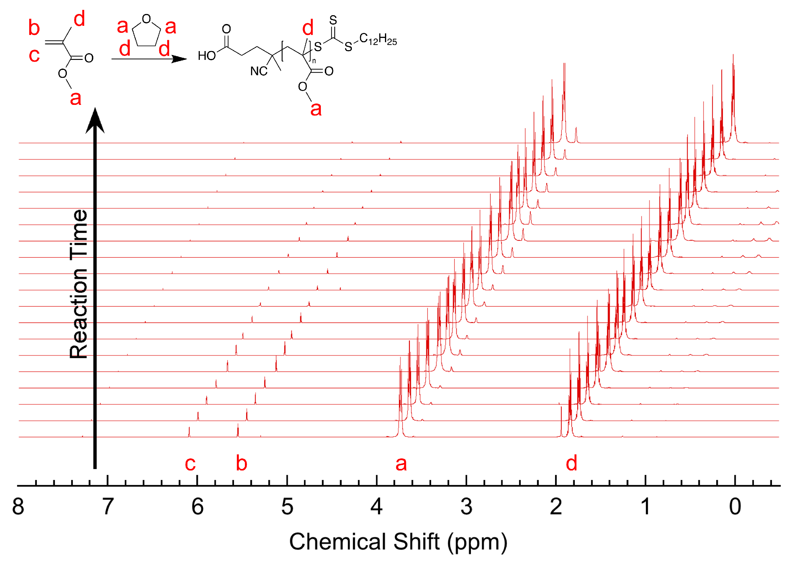
3.1. Materials and Methods

Materials. 4-cyano-4-(((dodecylthio)carbonothioyl)thio)pentanoic acid (chain transfer agent (CTA), 97%, Boron Molecular, Raleigh, NC, USA), tetrahydrofuran (THF, anhydrous, ≤99.9%, inhibitor-free, Sigma-Aldrich, Milwaukee, WI, USA), tetrahydrofuran (HPLC THF, inhibitor-free, for HPLC, ≤99.9%, Sigma-Aldrich, Milwaukee, WI, USA), tetrahydrofuran-d${}_8$ (THF-d${}_8$, ≤99.5% atom % D, Sigma-Aldrich, Milwaukee, WI, USA), chloroform-d (CDCl${}_3$, 99.96 atom % D, contains 0.03% (v/v) TMS, Sigma-Aldrich, Milwaukee, WI, USA), and methanol (MeOH, ACS reagent, ≤99.8%, Sigma-Aldrich, Milwaukee, WI, USA) were used as received. Azobis(isobutyronitrile) (AIBN, 98%, Sigma-Aldrich, Milwaukee, WI, USA) was purified via recrystallization twice from methanol. Methyl methacrylate (MMA, 99%, contains ≤30 ppm MEHQ as inhibitor, Sigma-Aldrich, Milwaukee, WI, USA) was purified by distillation over CaH${}_2$ at a reduced pressure.

Characterization. The molecular weights and dispersitys of all polymers and reacting mixture aliquots were determined by size exclusion chromatography (SEC) using a Waters GPC system (Milford, MA, USA) equipped with a THF Styragel column (Styragel@HR 5E, effective separation of molecular weight range: 2–4000 kg mol${}^{-1}$) and a 2414 reflective index (RI) detector. All measurements were performed at 40 ${}^{\circ }$C, where THF was used as the mobile phase at a flow rate of 1.0 mL min${}^{-1}$. Poly(styrene) standards (Shodex, Tokyo, Japan) with molecular weights ranging from 2.97 to 983 kg mol${}^{-1}$ were used for calibration. Molecular weight values determined against the poly(styrene) standards were converted to the true poly(methyl methacrylate) values using the Universal Calibration procedure. Chemical structures of all polymers and reacting mixture aliquots from large-scale reactions were characterized by ${}^1$H NMR (Nuclear Magnetic Resonance) Spectroscopy using a Bruker Avance 500 MHz spectrometer (Billerica, MA, USA) at 23 ${}^{\circ }$C with CDCl${}_3$ as the solvent. The chemical shifts were referenced to chloroform at 7.27 ppm. Small-scale PMMA macro-CTA reactions were characterized by ${}^1$H NMR spectroscopy using a Varian NMRS 500 MHz spectrometer (Palo Alto, CA, USA) at 60 ${}^{\circ }$C with THF-d${}_8$ as the solvent. The chemical shifts were referenced to THF at 1.73 ppm.

Polymer Synthesis Procedures. Two synthesis scales were executed in this work: large-scale and small-scale reactions. Large-scale reactions (>400 mL) consisted of a reflux reactor, which allowed for the removal of reacting mixture via aliquots during the reaction with negligible effect on the reacting volume. All aliquots were analyzed by ${}^1$H NMR spectroscopy and SEC. Small-scale reactions (<2 mL) consisted of reactions occurring in sealable temperature-controlled NMR tubes, where frequent in situ NMR analysis of the reacting mixture is possible without collecting aliquots from the reactor. SEC analysis of small-scale reactions were only conducted on the final product.

Large-Scale Reaction Procedure. A general procedure for large-scale polymer synthesis in a reflux reactor is outlined here with reaction details for each reaction listed in

Table 4. Reaction conditions for all polymerization reactions.

Reaction ${}^{\mathit{a}}$	Scale	Recipe ${}^{\mathit{b}}$	Monomer (g)	CTA (g)	Initiator (g)	Solvent (g) ${}^{\mathit{c}}$
PMMA-1	Large	215:1:0.1	250.63	4.7	0.191	626.58
PMMA-2	Large	70:1:0.1	173.62	10.0	0.407	714.48
PMMA-3	Small	215:1:0.1	0.5333	0.01	0.0004	1.3331
PMMA-4	Small	70:1:0.1	0.3472	0.02	0.0008	0.8681

${}^a$ Polymer-reaction number. ${}^b$ A:B:C = Monomer:CTA:Initiator (in mol). ${}^c$ THF-d${}_8$ was used for PMMA small-scale reactions.

. Monomer and CTA were mixed with solvent in a 2000 mL three-neck round-bottom flask, where the central neck of the flask was connected to a reflux condenser (connected to bubbler and a nitrogen source from a Schlenk line) and the other two necks of the flask were sealed with rubber septa. The reacting mixture was degassed by bubbling nitrogen gas through the reacting mixture for 2 h. After degassing, the reactor was placed into an oil bath, covered in aluminum foil, and heated to reflux. In a separate 10 mL vial sealed with a septum, the initiator was dissolved in solvent and degassed by bubbling nitrogen gas through the solution for 5 min. At the first sign of reflux, the degassed initiator solution was injected into the reacting mixture, and a 1 mL aliquot was collected from the reactor for ${}^1$H NMR and SEC analysis. The reaction was carried out under reflux for seven days. Additional aliquots were collected throughout the reaction for analysis. The resulting polymer was twice precipitated dropwise in methanol, filtered, and then dried under dynamic vacuum in an oven at room temperature for 24 h.

Small-Scale Reaction Procedure. A general procedure for small-scale polymer synthesis in an NMR tube reactor is outlined here with reaction details for each reaction listed in Table 4. Monomer, CTA and initiator were mixed with solvent in a sealable low pressure/vacuum NMR tube, connected to a nitrogen Schlenk line, and subjected to four freeze-pump-thaw degassing cycles. After degassing, the NMR tube was sealed under a nitrogen environment. The NMR tube reactor was inserted into a Varian NMRS 500 MHz NMR spectrometer at 60 ${}^{\circ }$C for 23 h, where NMR spectra were collected every 10 min. The resulting polymer was twice precipitated in methanol, filtered, and then dried under dynamic vacuum in an oven at room temperature for 24 h.

Synthesis of Poly(methyl methacrylate). The synthesis of poly(methyl methacrylate) (PMMA) macro-CTA is shown in Scheme 2. In total, four PMMA synthesis reactions were performed: two large-scale and two small-scale reactions. Reaction details for each reaction are listed in Table 4. Product details for each reaction are listed in

Table 5. Final product properties for all polymerization reactions.

Reaction ${}^{\mathit{a}}$	Scale	Recipe ${}^{\mathit{b}}$	Yield (g)	M${}_{\mathbf{n}}$ (g mol${}^{-1}$) ${}^{\mathit{c}}$	M${}_{\mathbf{w}}$ (g mol${}^{-1}$) ${}^{\mathit{c}}$	Đ ${}^{\mathit{c}}$
PMMA-1	Large	215:1:0.1	240 (94%)	21121	26347	1.247
PMMA-2	Large	70:1:0.1	158 (86%)	7877	10025	1.273
PMMA-3	Small	215:1:0.1	-	11971	14698	1.228
PMMA-4	Small	70:1:0.1	-	6669	8101	1.215

${}^a$ Polymer-reaction number. ${}^b$ A:B:C = Monomer:CTA:Initiator (in mol). ${}^c$ Determined by SEC.

. Monomer: MMA; solvent: THF; initiator: AIBN. ${}^1$H NMR (500 MHz, CDCl${}_3$, 23 ${}^{\circ }$C) $\delta$ (ppm): 3.57 (s, 3H, O-CH${}_3$), 1.84-1.76 (d, 2H, CH${}_2$-C(CH${}_3$)), 0.94-0.74 (d, 3H, CH${}_2$-C(CH${}_3$)).

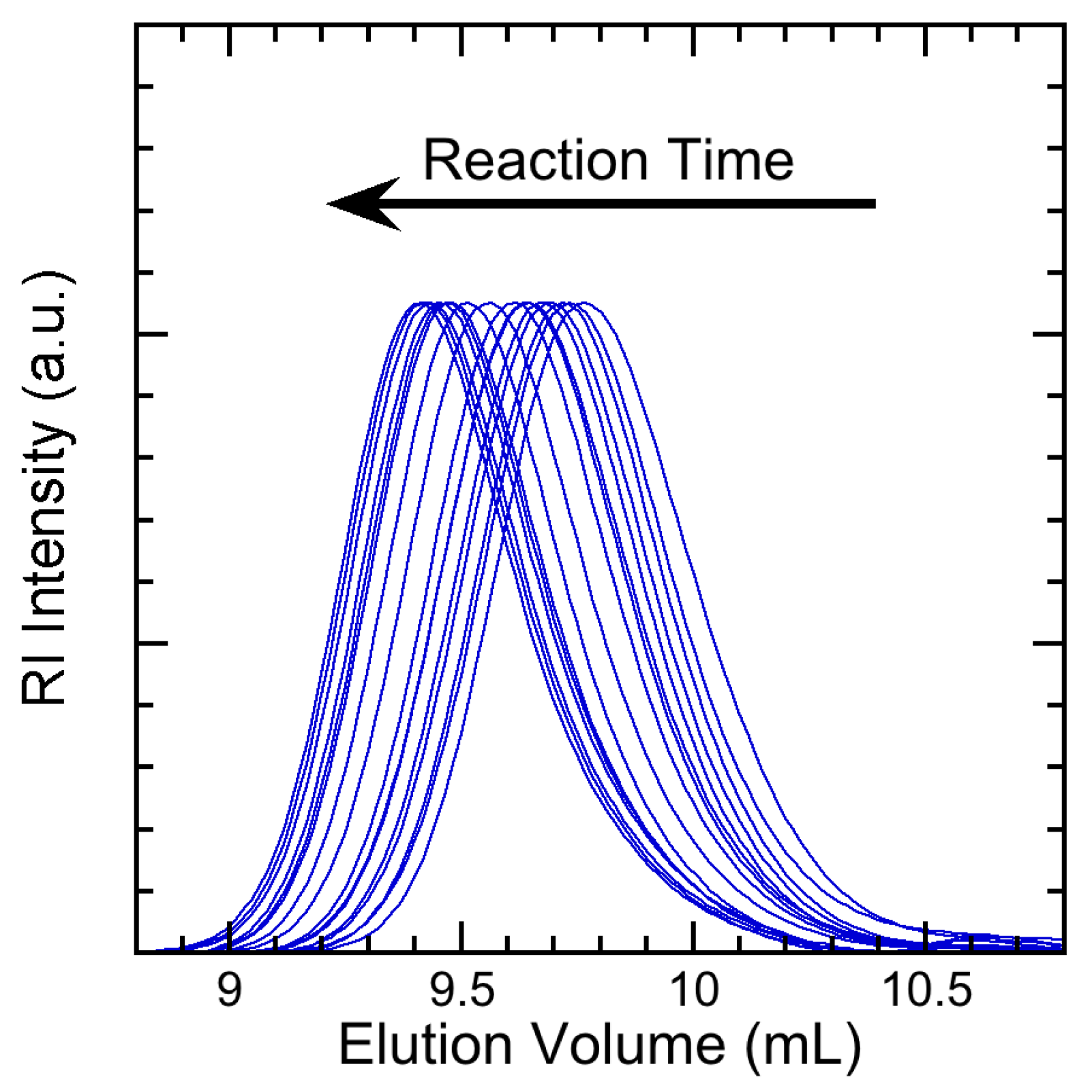
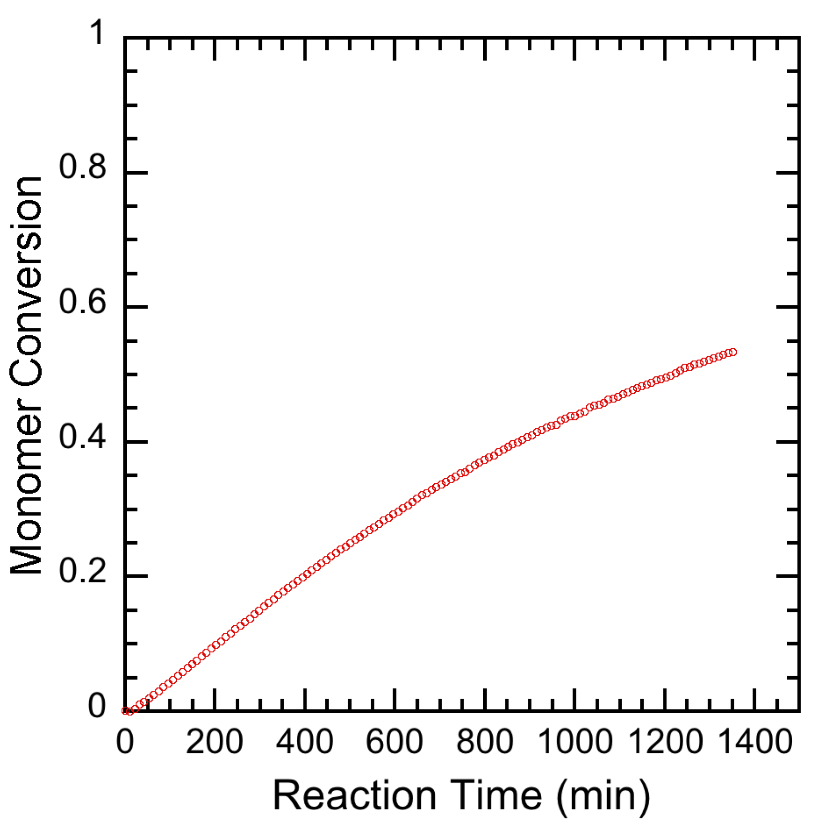
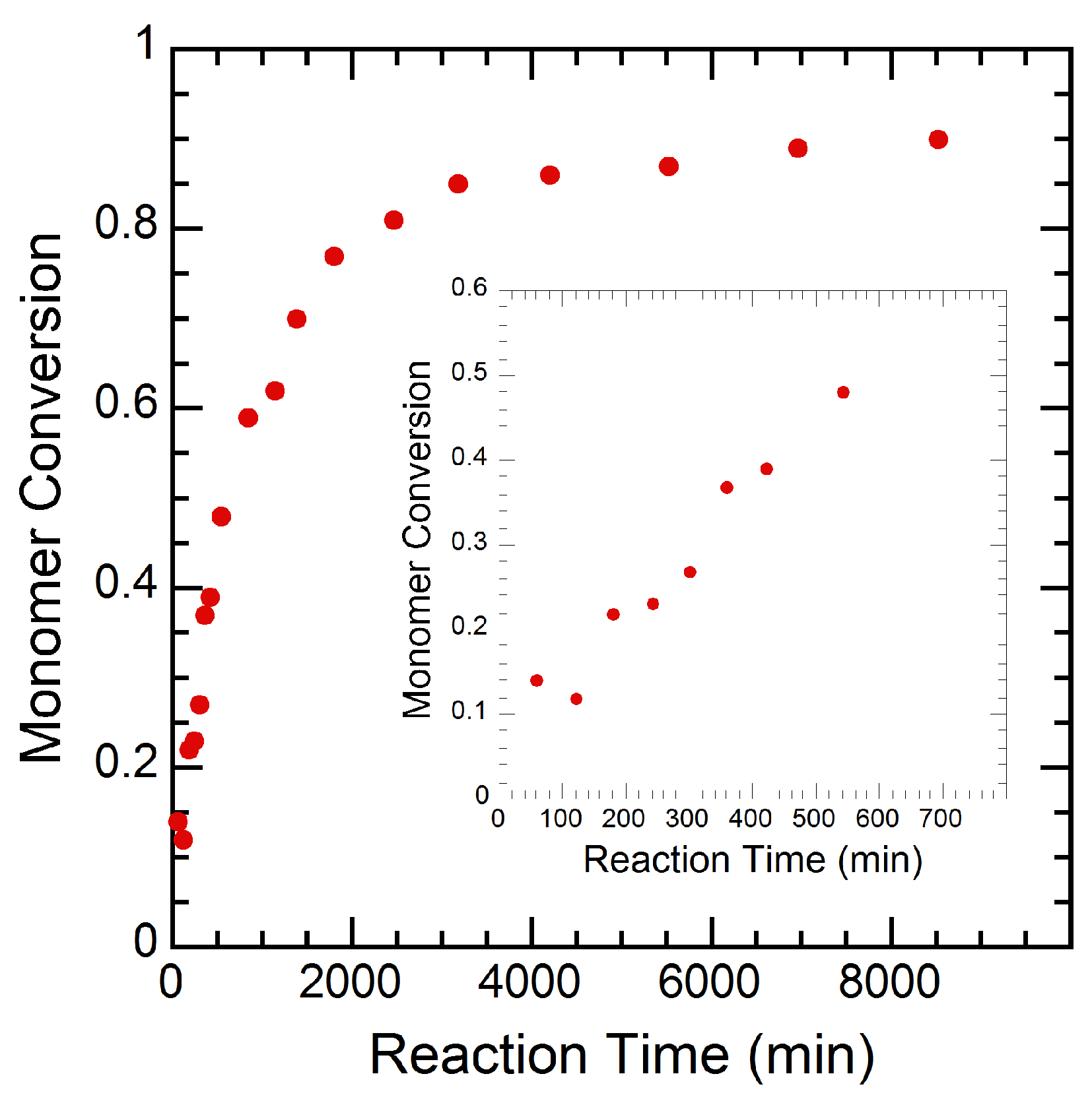
3.2. Experimental Results

Figure 2 shows the SEC profiles for large-scale reaction of PMMA (PMMA-1) as a function of time. Data only after 240 min is shown as aliquots at earlier times did not precipitate due to low monomer conversion. Molecular weights and dispersity data were calculated from the SEC data for all aliquots (all time points) and are listed in Appendix A (

Table A1. Summary of ${}^1$H NMR and SEC data for PMMA-1.

Time (h)	Time (min)	NMR Conv. (%)	SEC Conv. (%)	M${}_{\mathbf{n}}$ (g mol${}^{-1}$)	M${}_{\mathbf{w}}$ (g mol${}^{-1}$)	Đ ${}^{\mathit{a}}$	DP ${}^{\mathit{b}}$
0	0	0	-	-	-	-	-
0.5	30	5	-	-	-	-	-
1	60	9	-	-	-	-	-
1.5	90	11	-	-	-	-	-
2	120	15	-	-	-	-	-
3	180	21	42.9	9637	12,409	1.288	92
4	240	26	27.5	6324	9949	1.573	59
5	300	31	41.5	9334	13,227	1.417	89
6	360	33	50.4	11,261	13,954	1.239	108
7	420	38	53.5	11,927	14,858	1.246	115
8	480	41	55.6	12,383	15,382	1.242	120
10	600	47	56.3	12,523	15,800	1.262	121
13	780	59	60.1	13,346	17,018	1.275	129
17	1020	59	64.5	14,293	17,964	1.257	139
22	1320	64	68.9	15,240	19,357	1.270	148
33	1980	75	79.7	17,560	21,400	1.219	171
47	2820	81	85.1	18,724	22,974	1.227	183
58	3480	85	86.2	18,957	23,296	1.229	185
66	3960	87	86.6	19,052	23,744	1.246	186
90	5400	91	91.5	20,107	25,067	1.247	197
114	6840	94	94.9	20,824	25,766	1.237	204
143	8580	95	96.2	21,121	26,347	1.247	207

${}^a$ Đ = dispersity; ${}^b$ DP = degree of polymerization.

) for PMMA-1 and the other large-scale polymerization reaction (PMMA-2:

Table A2. Summary of ${}^1$H NMR and SEC data for PMMA-2.

Time (h)	Time (min)	NMR Conv. (%)	SEC Conv. (%)	M${}_{\mathbf{n}}$ (g mol${}^{-1}$)	M${}_{\mathbf{w}}$ (g mol${}^{-1}$)	Đ ${}^{\mathit{a}}$	DP ${}^{\mathit{b}}$
0	0	0	-	-	-	-	-
1	60	14	23.4	2042 ${}^c$	2990 ${}^c$	1.464	16
2	120	12	34.4	2814 ${}^c$	3918 ${}^c$	1.392	24
3	180	22	40.0	3208 ${}^c$	4433 ${}^c$	1.382	28
4	240	23	48.1	3777	5055	1.338	34
5	300	27	53.6	4162	5604	1.346	38
6	360	37	55.5	4292	5910	1.377	39
7	420	39	58.1	4472	6122	1.369	41
9	540	48	81.5	6112	7877	1.289	57
14	840	59	90.7	6759	8496	1.257	63
19	1140	62	94.2	7003	8672	1.238	66
23	1380	70	104.1	7698	9203	1.195	73
30	1800	77	101.2	7497	9304	1.241	71
41	2460	81	104.9	7754	9620	1.241	73
53	3180	85	108.9	8035	9809	1.221	76
70	4200	86	104.2	7704	9671	1.255	73
92	5520	87	109.1	8051	9933	1.234	76
116	6960	89	106.0	7834	9893	1.263	74
142	8520	90	106.6	7877	10,025	1.273	75

${}^a$ Đ = dispersity; ${}^b$ DP = degree of polymerization; ${}^c$ These values are below the lower calibration limit of the SEC and determined by extrapolating the calibration curve to the corresponding elution volumes.

). The SEC profiles clearly shift to earlier elution volumes at later reaction times, indicating the growth of polymer chains throughout the reaction. Molecular weight increases from an M${}_{\mathrm{n}}$ of 6,324 Da at 240 min to an M${}_{\mathrm{n}}$ of 21,121 Da at 8,580 min. Dispersity is well controlled throughout the reaction as shown by the minimal change in the breadth of the profiles and dispersities less than 1.3 for all profiles except for the profiles at reaction times of 240 min and 300 min. High dispersities at low monomer conversions (i.e., early reaction times) are expected in RAFT polymerization reactions. Chromatogram profiles form a tail at high elution volumes at later reaction times signifying the formation of dead polymer chains due to termination reactions.

Figure 3 shows the corresponding ${}^1$H NMR spectra for all aliquots for the large-scale PMMA reaction (PMMA-1). Analysis of these spectra provides monomer conversion data, which is listed for each time point in Appendix A (Table A1) for PMMA-1 and the other large-scale polymerization reaction (PMMA-2: Table A2). Four primary bands are visible (a, b, c and d) in each spectrum and were subsequently integrated. Monomer conversion was calculated from comparing integral of band b at specified time to integral of band b at t = 0, where integral of band a was set as the reference. Monomer conversion ranges from 0% at 0 min to 95% at 8,580 min.

Figure 4 shows the polymerization kinetics data as calculated by the ${}^1$H NMR analysis in Figure 3. Tabulated results are listed in Appendix A (Table A1) for PMMA-1 and the other large-scale polymerization reaction (PMMA-2: Table A2).

Figure 5 shows the polymerization kinetics as calculated by NMR analysis for the small-scale PMMA polymerization (PMMA-3). The NMR spectra for PMMA-3 were processed similar to the procedure described for PMMA-1. Using THF-d${}_8$ in PMMA-3 instead of THF in PMMA-1 did not affect the NMR spectra processing procedure. The data appears to follow first order reaction kinetics similar to the large-scale reaction results.

Data for the other polymerization reactions (PMMA-2, PMMA-4) is available in Appendix A.

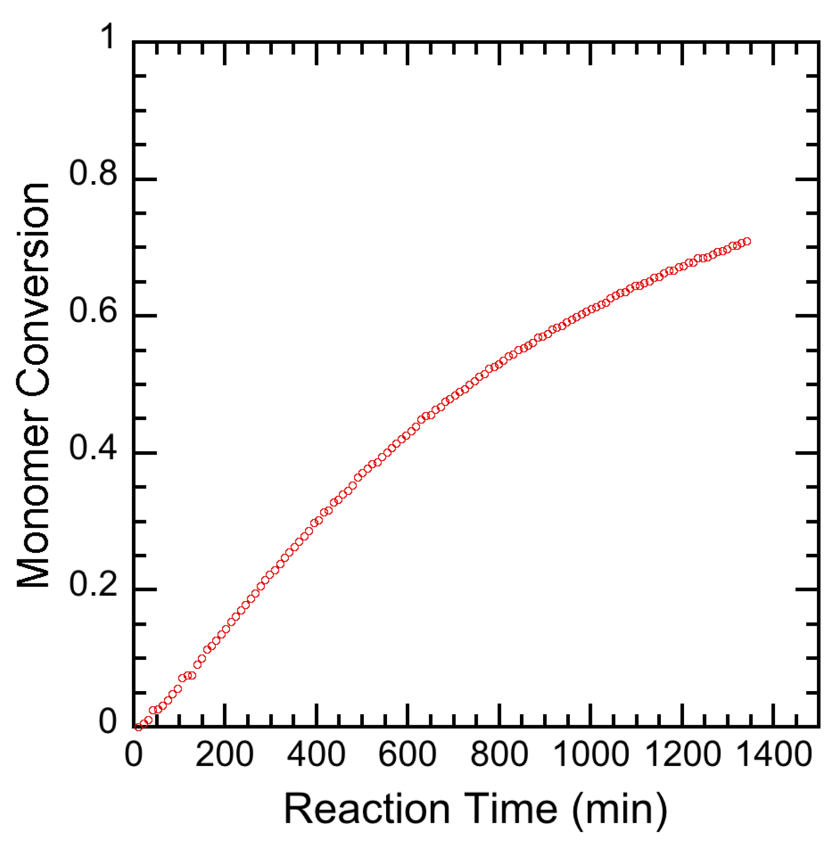
4. Results and Discussion

In this part, the results for both model fitting and the multi-rate multi-delay observer will be demonstrated. The small-scale experiment results, which contain 127 conversion data points measured using ${}^1$H NMR and 1 ending data point measured with SEC for both PMMA-3 and PMMA-4 sets, are used for parameter fitting purposes. The two sets of large-scale experimental results, with fewer but more comprehensive and practical sampled data points, are to be used to validate the calculated parameters. The observer will be designed based on the fitted model and tested on one of the large-scale reaction data sets.

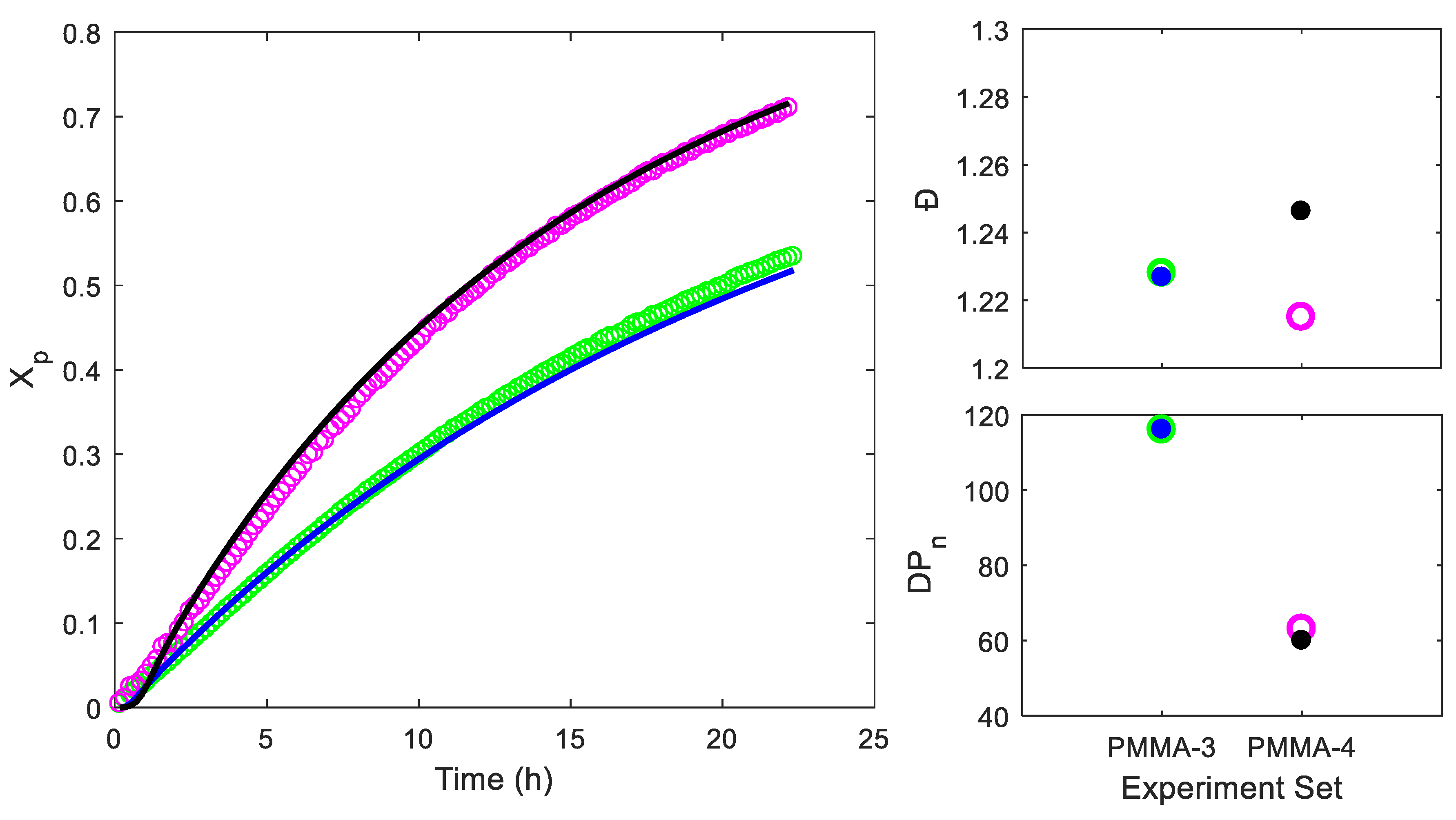
4.1. Parameter Fitting

For the model (2) introduced in Section 2, values of the parameters for some specific experiments have been identified by other researchers as shown in Table 3. With regards to the experimental setting introduced in Section 3, a RAFT agent is used for which no kinetics data was found in literature. Therefore, its kinetic characteristics remain unknown. Additionally, initiator efficiency varies in different environments and must be identified. Therefore, there are five parameters for the current system to be fitted: the forward RAFT main equilibrium reaction rate coefficient $k_{raftf}$, the reverse RAFT main equilibrium reaction rate coefficient $k_{raftr}$, the forward RAFT pre-equilibrium reaction rate coefficient $k_{raftfR}$, the reverse RAFT pre-equilibrium reaction rate coefficient $k_{raftrR}$, and the initiator efficiency f. While the small scale reaction is operated under a constant temperature of 60 ${}^{\circ }$C and the large scale reaction at the bubble point of the reaction mixture (65–80 ${}^{\circ }$C), it is assumed that the effect of temperature on these parameters is negligible over this range. This assumption, while not ideal, is necessary due to limitations in the reaction techniques. Small-scale reactions cannot be performed at reflux, and large-scale reactions must be performed at reflux. The small-scale reactions were performed as close to reflux temperature as possible without risking evaporation of solvent, and damage to the NMR.

Because the least squares parameter fitting problem is highly non-convex and non-smooth, the PatternSearch solver in MATLAB (version 9.7.0.1190202 (R2019b), MathWorks, Natick, MA, USA) with multiple random initial points is used to solve for the global optimal solution. In order to set up the optimization problem, an appropriate objective function is needed. It is preferable to use the variable that has a large number of sampled data in the objective function, which is the conversion $X_p$ in this case. However, it is observed that, when minimizing the error of conversion, in the basin region near the global optimum, the error becomes less sensitive to the fitting parameters. Additionally, the optimal solution could not guarantee whether the model also matches the SEC data. Thereby, the dispersity (Đ) and the number average degree of polymerization ($D{P}_n$) measured from SEC for the ending point are also used as a part of the objective function, and normalized to the proper scale with a weighting coefficient of 5 and $1/25$, respectively. The global optimal parameters are calculated as: $k_{raftf}=3.74\times {10}^4\mathrm{L}/(\mathrm{mol}·\mathrm{s})$, $k_{raftr}=1.82/\mathrm{s}$, $k_{raftfR}=9.34\times {10}^6\mathrm{L}/(\mathrm{mol}·\mathrm{s})$, $k_{raftrR}=8.75/\mathrm{s}$ and $f=0.323$. These values match the typical values found in the literature [60].

Figure 6 shows the experimental data obtained from the small-scale in situ ${}^1$H NMR experiments, as well as the obtained fits which give the best estimation of the fitting parameters using least squares. It can be observed that the fitting model shows excellent agreement with the $X_p$ measurement. As for the single sampled Đ and $D{P}_n$ points on the right two plots, the estimated values from the model also match the experimental data well, especially for the PMMA-3 set.

For validation purposes, we test the model against two large-scale reaction sets (PMMA-1 and PMMA-2) in Figure 7. The measurement of conversion $X_p$ is obtained from ${}^1$H NMR measurement. The $D{P}_n$ and Đ data are collected from SEC measurement. The large-scale reactions are operated under reflux. The temperature is simulated as a function of the composition and used for the calculation of reaction kinetics coefficients except for $k_{raftf}$, $k_{raftr}$, $k_{raftfR}$ and $k_{raftrR}$, which are assumed to be independent of temperature.

Overall, the model satisfactorily matches the experimental data. Monomer conversion ($X_p$) and degree of polymerization ($D{P}_n$) match well at early reaction times, with some discordance appearing at late reaction times, especially for PMMA-1. The discordance may be due to temperature effects which are unaccounted for in the model due to the assumption that $k_{raftf}$, $k_{raftr}$, $k_{raftfR}$ and $k_{raftrR}$ are not functions of temperature. The large-scale and small-scale experimental reactions were performed at temperatures as close to each other as experimentally possible, but there was still a 10 to 15 ${}^{\circ }$C difference between the two reaction scales. Dispersities (Đ) match well, with the sharp peak around $Đ=2$ in the model at early times expected from typical RAFT polymerization. SEC data at early reaction times is not available for comparison because the corresponding reaction aliquots did not precipitate due to low monomer conversion.

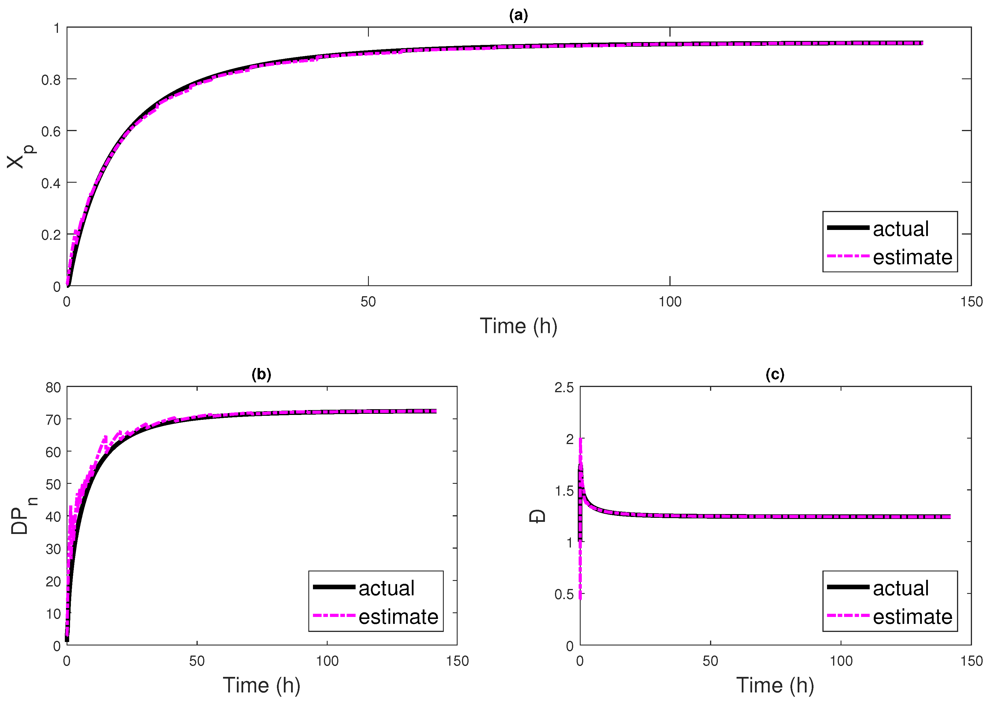
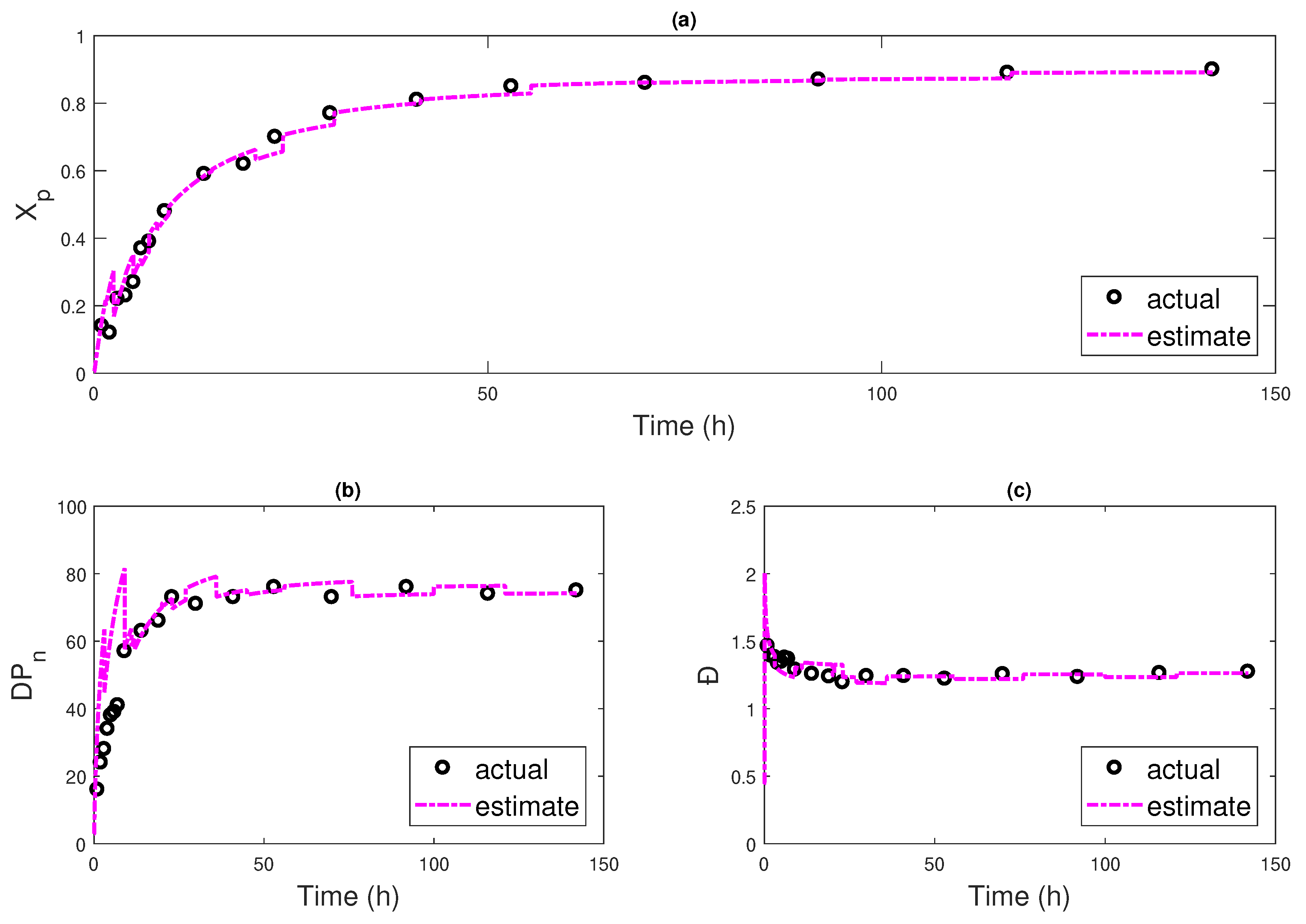
4.2. Multi-Rate Multi-Delay Observer

In this part, we test the multi-rate multi-delay observer proposed in Section 2.2.2 against both the fitting model and the experimental data, to check its fidelity to the model and its performance under real circumstances in the presence of errors.

The data set collected from the PMMA-2 large-scale experiment is used to test the design of the observer, as this data set shows a better consistence with the fitting model than the data set from the PMMA-1 large-scale experiment. During the reaction, aliquots were collected approximately every 5% monomer conversion, which resulted in a non-uniform sampling schedule with respect to time. The sampling schedule for the reaction and the delays in measurement for those samples are shown in

Table 6. Actual sampling schedule and measurement delays in the large-scale reactor.

Sampling (h)	1	2	3	4	5	6	7	9	14	19	23	30	41	53	70	92	116	142
SEC delay (h)	2	3	3	4	4	5	5	6	6	4	4	6	4	3	6	8	5	4
NMR delay (h)	0.5	0.5	1	1	1	1	0.5	1	1.5	1	0.5	0.5	2.5	1	0.5	0.5	1.5	1

.

In Figure 8, simulated data generated from the model is used as the measurement to test the observer’s performance against the fitting model with the same sampling schedule as shown in Table 6. The observer shows good prediction for monomer conversion, as the measurement from NMR has less delay than the measurement from SEC. The estimated $D{P}_n$ undergoes a period of oscillation and Đ shows a higher peak than the actual data, due to the fact that the first measurement from SEC only becomes available 3 h after the reaction starts. However, the prediction shows higher accuracy after a few samplings.

In Figure 9, the observer is designed based on real experimental data, and the comparison between estimated values from this observer and the sampled points is demonstrated. In these figures, the plotted estimation only shows the real-time information at each moment, and does not reflect the updated historical estimation for the past delayed time period that is corrected by the dead-time compensator later on. As a result, the magenta line does not go through the black measured points, but leaps to the levels corresponding to the newest sampling data after certain delays, with the dead-time compensator correction effects applied. Because the experimental data points themselves are fluctuating with measurement noises and the fitted model already shows deviation from the real samples, the performance of the observer is not as good as in Figure 8, in terms of a slower convergence rate and fluctuation at early reaction times. However, the observer still predicts conversion and dispersity with high accuracy after more sampling points become available.

5. Conclusions

In this work, a RAFT polymerization model was improved using small-scale reactions with in situ ${}^1$H NMR analysis that allowed for more accurate prediction of RAFT reaction kinetic rate parameters (specifically, $k_{raftf}$, $k_{raftr}$, $k_{raftfR}$ and $k_{raftrR}$). The resulting model with the fitted parameters was used to predict RAFT reactions on a larger scale with differing initial conditions to high values of monomer conversion, $X_p$. The fitted model accurately predicted the polymer properties of the large-scale reactions with slight discordance at late reaction times. Finally, multi-rate, multi-delay observers were used to more accurately monitor a reaction and its product’s quality in real time by incorporating information from the sampled and delayed measurements. The observer was tested both against the fitted model and the experimental data. At early reaction times, both observers show some deviations due to limited characterization data. However, at later reaction times, the observer against the fitted model shows perfect convergence, while the one based on the experimental data matches well with slight shifts upon receiving new measurements, owing to the inherent noises of the analysis techniques. Ultimately, accurate monitoring allowed for targeted termination, making it easier to synthesize polymers of desired properties.

RAFT polymerization is very versatile, being compatible with a wide array of monomer and RAFT agent types. In this work, a trithiocarbonate RAFT agent was used; however, other types, such as dithiocarbonates, are also common. Certain RAFT agents work better with certain monomer types; and now some RAFT agents, such as pyrazole based RAFT agents, even work effectively with all monomer types viable for RAFT polymerization. The methodology presented in this work for monitoring RAFT polymerization reactions could be applied to different monomer-RAFT agent combinations, allowing for monitoring of RAFT polymerizations in general.

In this work, the small-scale reactions used for the parameter fitting occurred at a different temperature than the large-scale reactions, due to limitations in the experimental apparatus and procedures. The temperature difference leads to some discordance when comparing the model to the large-scale reaction results. This discordance is attributed to the temperature difference. Large-scale reactions occur at a slightly higher temperature than the small-scale reactions, and would be expected to exhibit larger reaction rate constants. The methodology to determine the values of the RAFT reaction rate coefficients can be improved by determining temperature dependent reaction rate constant values. Further studies with multiple small-scale reactions at various temperatures can be performed to determine the temperature dependence of the RAFT reaction rate constants.

Additionally, as a living polymerization, polymers synthesized via RAFT polymerization are able to be chain extended into block copolymers. The block copolymers can be synthesized with different monomers with controlled block composition, while maintaining low dispersity. Block copolymers synthesized in this fashion have many applications due to the multiple properties. Many of these properties, such as morphology, depend on the block composition ratios, giving importance to targeting precise block composition during synthesis. Future work in this area would include modeling and monitoring these chain-extension polymerizations using a polymer reactant synthesized via RAFT polymerization. The resulting block copolymer compositions can be targeted, based on desired block copolymer properties, by using the observer based RAFT polymerization model to accurately predict reaction termination times and conditions.

References

1. Moad, G.; Chiefari, J.; Chong, Y.K.; Krstina, J.; Mayadunne, R.T.A.; Postma, A.; Rizzardo, E.; Thang, S.H. Living free radical polymerization with reversible addition–fragmentation chain transfer (the life of RAFT). Polym. Int. 2000, 49, 993–1001. [Google Scholar] [CrossRef]
2. Krstina, J.; Moad, C.L.; Moad, G.; Rizzardo, E.; Berge, C.T.; Fryd, M. A new form of controlled growth free radical polymerization. In Macromolecular Symposia; Hüthig & Wepf Verlag: Basel, Switzerland, 1996; Volume 111, pp. 13–23. [Google Scholar]
3. Gardiner, J.; Martinez-Botella, I.; Tsanaktsidis, J.; Moad, G. Dithiocarbamate RAFT agents with broad applicability - the 3,5-dimethyl-1H-pyrazole-1-carbodithioates. Polym. Chem. 2016, 7, 481–492. [Google Scholar] [CrossRef]
4. Gardiner, J.; Martinez-Botella, I.; Kohl, T.M.; Krstina, J.; Moad, G.; Tyrell, J.H.; Coote, M.L.; Tsanaktsidis, J. 4-Halogeno-3,5-dimethyl-1H-pyrazole-1-carbodithioates: Versatile reversible addition fragmentation chain transfer agents with broad applicability. Polym. Int. 2017, 66, 1438–1447. [Google Scholar] [CrossRef]
5. Moad, G. RAFT Polymerization—Then, and Now. In Controlled Radical Polymerization: Mechanisms; American Chemical Society: Akron, OH, USA, 2015; Volume 1187, pp. 211–246. [Google Scholar]
6. Ye, Y.S.; Choi, J.H.; Winey, K.I.; Elabd, Y.A. Polymerized Ionic Liquid Block and Random Copolymers: Effect of Weak Microphase Separation on Ion Transport. Macromolecules 2012, 45, 7027–7035. [Google Scholar] [CrossRef]
7. Stace, S.J.; Fellows, C.M.; Moad, G.; Keddie, D.J. Effect of the Z- and Macro-R-Group on the Thermal Desulfurization of Polymers Synthesized with Acid/Base “Switchable” Dithiocarbamate RAFT Agents. Macromol. Rapid Commun. 2018, 39, e1800228. [Google Scholar] [CrossRef]
8. Chiefari, J.; Mayadunne, R.T.A.; Moad, C.L.; Moad, G.; Rizzardo, E.; Postma, A.; Skidmore, M.A.; Thang, S.H. Thiocarbonylthio compounds (S=C(Z)S-R) in free radical polymerization with reversible addition–fragmentation chain transfer (RAFT polymerization). Effect of the activating group Z. Macromolecules 2003, 36, 2273–2283. [Google Scholar] [CrossRef]
9. Chiefari, J.; Chong, Y.; Ercole, F.; Krstina, J.; Jeffery, J.; Le, T.P.; Mayadunne, R.T.; Meijs, G.F.; Moad, C.L.; Moad, G.; et al. Living free-radical polymerization by reversible addition- fragmentation chain transfer: The RAFT process. Macromolecules 1998, 31, 5559–5562. [Google Scholar] [CrossRef]
10. Montgomery, K.S.; Davidson, R.W.M.; Cao, B.; Williams, B.; Simpson, G.W.; Nilsson, S.K.; Chiefari, J.; Fuchter, M.J. Effective macrophage delivery using RAFT copolymer derived nanoparticles. Polym. Chem. 2018, 9, 131–137. [Google Scholar] [CrossRef]
11. Nykaza, J.R.; Benjamin, R.; Meek, K.M.; Elabd, Y.A. Polymerized ionic liquid diblock copolymer as an ionomer and anion exchange membrane for alkaline fuel cells. Chem. Eng. Sci. 2016, 154, 119–127. [Google Scholar] [CrossRef]
12. Nykaza, J.R.; Savage, A.M.; Pan, Q.W.; Wang, S.J.; Beyer, F.L.; Tang, M.H.; Li, C.Y.; Elabd, Y.A. Polymerized ionic liquid diblock copolymer as solid-state electrolyte and separator in lithium-ion battery. Polymer 2016, 101, 311–318. [Google Scholar] [CrossRef] [Green Version]
13. Moehrke, J.; Vana, P. The Kinetics of Surface-Initiated RAFT Polymerization of Butyl acrylate Mediated by Trithiocarbonates. Macromol. Chem. Phys. 2017, 218, 1600506. [Google Scholar] [CrossRef]
14. Bates, F.S.; Fredrickson, G.H. Block copolymer thermodynamics: Theory and experiment. Annu. Rev. Phys. Chem. 1990, 41, 525–557. [Google Scholar] [CrossRef] [PubMed]
15. Zhang, M.; Ray, W.H. Modeling of “living” free-radical polymerization with RAFT chemistry. Ind. Eng. Chem. Res. 2001, 40, 4336–4352. [Google Scholar] [CrossRef]
16. Zetterlund, P.B.; Gody, G.; Perrier, S. Sequence-Controlled Multiblock Copolymers via RAFT Polymerization: Modeling and Simulations. Macromol. Theory Simul. 2014, 23, 331–339. [Google Scholar] [CrossRef]
17. Hernandez-Ortiz, J.C.; Jaramillo-Soto, G.; Palacios-Alquisira, J.; Vivaldo-Lima, E. Modeling of Polymerization Kinetics and Molecular Weight Development in the Microwave-Activated RAFT Polymerization of Styrene. Macromol. React. Eng. 2010, 4, 210–221. [Google Scholar] [CrossRef]
18. Barner-Kowollik, C.; Quinn, J.F.; Morsley, D.R.; Davis, T.P. Modeling the reversible addition–fragmentation chain transfer process in cumyl dithiobenzoate-mediated styrene homopolymerizations: Assessing rate coefficients for the addition–fragmentation equilibrium. J. Polym. Sci. Part A Polym. Chem. 2001, 39, 1353–1365. [Google Scholar] [CrossRef]
19. Wang, A.R.; Zhu, S.P. Effects of diffusion-controlled radical reactions on RAFT polymerization. Macromol. Theory Simul. 2003, 12, 196–208. [Google Scholar] [CrossRef]
20. Chaffey-Millar, H.; Busch, M.; Davis, T.P.; Stenzel, M.H.; Barner-Kowollik, C. Advanced computational strategies for modelling the evolution of full molecular weight distributions formed during multiarmed (Star) polymerisations. Macromol. Theory Simul. 2005, 14, 143–157. [Google Scholar] [CrossRef]
21. Tobita, H. Modeling Controlled/Living Radical Polymerization Kinetics: Bulk and Miniemulsion. Macromol. React. Eng. 2010, 4, 643–662. [Google Scholar] [CrossRef]
22. Lopez-Dominguez, P.; Hernandez-Ortiz, J.C.; Vivaldo-Lima, E. Modeling of RAFT Copolymerization with Crosslinking of Styrene/Divinylbenzene in Supercritical Carbon Dioxide. Macromol. Theory Simul. 2018, 27, 1700064. [Google Scholar] [CrossRef]
23. Vana, P.; Davis, T.P.; Barner-Kowollik, C. Kinetic analysis of reversible addition fragmentation chain transfer (RAFT) polymerizations: Conditions for inhibition, retardation, and optimum living polymerization. Macromol. Theory Simul. 2002, 11, 823–835. [Google Scholar] [CrossRef]
24. Adebekun, D.K.; Schork, F.J. Continuous solution polymerization reactor control. 2. Estimation and nonlinear reference control during methyl methacrylate polymerization. Ind. Eng. Chem. Res. 1989, 28, 1846–1861. [Google Scholar] [CrossRef]
25. Jo, J.H.; Bankoff, S.G. Digital monitoring and estimation of polymerization reactors. AIChE J. 1976, 22, 361–369. [Google Scholar] [CrossRef]
26. Kim, K.J.; Choi, K.Y. On-line estimation and control of a continuous stirred tank polymerization reactor. J. Process Control 1991, 1, 96–110. [Google Scholar] [CrossRef]
27. Ellis, M.F.; Taylor, T.W.; Jensen, K.F. On-line molecular weight distribution estimation and control in batch polymerization. AIChE J. 1994, 40, 445–462. [Google Scholar] [CrossRef]
28. Crowley, T.J.; Choi, K.Y. On-line monitoring and control of a batch polymerization reactor. J. Process Control 1996, 6, 119–127. [Google Scholar] [CrossRef]
29. Mutha, R.K.; Cluett, W.R.; Penlidis, A. On-line nonlinear model-based estimation and control of a polymer reactor. AIChE J. 1997, 43, 3042–3058. [Google Scholar] [CrossRef]
30. Dimitratos, J.; Georgakis, C.; El-Aasser, M.S.; Klein, A. Dynamic modeling and state estimation for an emulsion copolymerization reactor. Comput. Chem. Eng. 1989, 13, 21–33. [Google Scholar] [CrossRef]
31. Kozub, D.J.; MacGregor, J.F. State estimation for semi-batch polymerization reactors. Chem. Eng. Sci. 1992, 47, 1047–1062. [Google Scholar] [CrossRef]
32. Astorga, C.M.; Sheibat-Othman, N.; Othman, S.; Hammouri, H.; McKenna, T.F. Nonlinear continuous-discrete observers: Application to emulsion polymerization reactors. Control Eng. Pract. 2002, 10, 3–13. [Google Scholar] [CrossRef]
33. Appelhaus, P.; Engell, S. Design and implementation of an extended observer for the polymerization of polyethylenterephthalate. Chem. Eng. Sci. 1996, 51, 1919–1926. [Google Scholar] [CrossRef]
34. Van Dootingh, M.; Viel, F.; Rakotopara, D.; Gauthier, J.P.; Hobbes, P. Nonlinear deterministic observer for state estimation: Application to a continuous free radical polymerization reactor. Comput. Chem. Eng. 1992, 16, 777–791. [Google Scholar] [CrossRef]
35. Viel, F.; Busvelle, E.; Gauthier, J.P. Stability of polymerization reactors using I/O linearization and a high-gain observer. Automatica 1995, 31, 971–984. [Google Scholar] [CrossRef]
36. Tatiraju, S.; Soroush, M. Nonlinear state estimation in a polymerization reactor. Ind. Eng. Chem. Res. 1997, 36, 2679–2690. [Google Scholar] [CrossRef]
37. Tatiraju, S.; Soroush, M.; Ogunnaike, B.A. Multirate nonlinear state estimation with application to a polymerization reactor. AIChE J. 1999, 45, 769–780. [Google Scholar] [CrossRef]
38. Soroush, M. State and parameter estimations and their applications in process control. Comput. Chem. Eng. 1998, 23, 229–245. [Google Scholar] [CrossRef]
39. López-Negrete, R.; Biegler, L.T. A Moving Horizon Estimator for processes with multi-rate measurements: A Nonlinear Programming sensitivity approach. J. Process Control 2012, 22, 677–688. [Google Scholar] [CrossRef]
40. Krämer, S.; Gesthuisen, R. Multirate state estimation using moving horizon estimation. In Proceedings of the 16th IFAC World Conference (IFAC 2005), Prague, Czech Republic, 3–8 July 2005; pp. 1–6. [Google Scholar]
41. Liu, A.; Zhang, W.; Yu, L.; Chen, J. Moving horizon estimation for multi-rate systems. In Proceedings of the 54th IEEE Conference on Decision and Control, Osaka, Japan, 15–18 December 2015; pp. 6850–6855. [Google Scholar]
42. Zambare, N.; Soroush, M.; Grady, M.C. Real-time multirate state estimation in a pilot-scale polymerization reactor. AIChE J. 2002, 48, 1022–1033. [Google Scholar] [CrossRef]
43. Ling, C.; Kravaris, C. State observer design for monitoring the degree of polymerization in a series of melt polycondensation reactors. Processes 2016, 4, 4. [Google Scholar] [CrossRef]
44. Kahelras, M.; Ahmed-Ali, T.; Giri, F.; Lamnabhi-Lagarrigue, F. Sampled-data chain-observer design for a class of delayed nonlinear systems. Int. J. Control 2018, 91, 1076–1090. [Google Scholar] [CrossRef]
45. Ahmed-Ali, T.; Karafyllis, I.; Lamnabhi-Lagarrigue, F. Global exponential sampled-data observers for nonlinear systems with delayed measurements. Syst. Control Lett. 2013, 62, 539–549. [Google Scholar] [CrossRef] [Green Version]
46. Nadri, M.; Hammouri, H. Design of a continuous-discrete observer for state affine systems. Appl. Math. Lett. 2003, 16, 967–974. [Google Scholar] [CrossRef]
47. Karafyllis, I.; Kravaris, C. From continuous-time design to sampled-data design of observers. IEEE Trans. Autom. Control 2009, 54, 2169–2174. [Google Scholar] [CrossRef]
48. Zambare, N.; Soroush, M.; Ogunnaike, B.A. A method of robust multi-rate state estimation. J. Process Control 2003, 13, 337–355. [Google Scholar] [CrossRef]
49. Antoniades, C.; Christofides, P.D. Feedback control of nonlinear differential difference equation systems. Chem. Eng. Sci. 1999, 54, 5677–5709. [Google Scholar] [CrossRef]
50. Liu, J.; Muñoz de la Peña, D.; Christofides, P.D.; Davis, J.F. Lyapunov-based model predictive control of nonlinear systems subject to time-varying measurement delays. Int. J. Adapt. Control Signal Process. 2009, 23, 788–807. [Google Scholar] [CrossRef]
51. Liu, J.; Muñoz de la Peña, D.; Christofides, P.D. Distributed model predictive control of nonlinear systems subject to asynchronous and delayed measurements. Automatica 2010, 46, 52–61. [Google Scholar] [CrossRef]
52. Ling, C.; Kravaris, C. Multi-rate observer design using asynchronous inter-sample output predictions. In Proceedings of the 2017 American Control Conference (ACC), Seattle, WA, USA, 24–26 May 2017; pp. 376–381. [Google Scholar]
53. Ling, C.; Kravaris, C. Multi-rate observer design for process monitoring using asynchronous inter-sample output predictions. AIChE J. 2017, 63, 3384–3394. [Google Scholar] [CrossRef]
54. Ling, C.; Kravaris, C. Multi-rate sampled-data observers based on a continuous-time design. In Proceedings of the 2017 IEEE 56th Annual Conference on Decision and Control (CDC), Melbourne, Australia, 12–15 December 2017; pp. 3664–3669. [Google Scholar]
55. Ling, C.; Kravaris, C. Multi-rate Sampled-data Observer Design for Nonlinear Systems with Asynchronous and Delayed Measurements. In Proceedings of the 2019 American Control Conference (ACC), Philadelphia, PA, USA, 10–12 July 2019; pp. 1128–1133. [Google Scholar]
56. Ling, C.; Kravaris, C. Multi-Rate Sampled-Data Observer Design Based on a Continuous-Time Design. IEEE Trans. Autom. Control. 2019. [Google Scholar] [CrossRef]
57. Ling, C.; Kravaris, C. A dead time compensation approach for multirate observer design with large measurement delays. AIChE J. 2019, 65, 562–570. [Google Scholar] [CrossRef]
58. Buback, M.; Kowollik, C. Termination kinetics of methyl methacrylate free-radical polymerization studied by time-resolved pulsed laser experiments. Macromolecules 1998, 31, 3211–3215. [Google Scholar] [CrossRef]
59. Beuermann, S.; Buback, M.; Davis, T.P.; Gilbert, R.G.; Hutchinson, R.A.; Olaj, O.F.; Russell, G.T.; Schweer, J.; Van Herk, A.M. Critically evaluated rate coefficients for free-radical polymerization, 2. Propagation rate coefficients for methyl methacrylate. Macromol. Chem. Phys. 1997, 198, 1545–1560. [Google Scholar] [CrossRef]
60. Moad, G.; Rizzardo, E.; Thang, S.H. Radical addition–fragmentation chemistry in polymer synthesis. Polymer 2008, 49, 1079–1131. [Google Scholar] [CrossRef]
61. Perrier, S.; Barner-Kowollik, C.; Quinn, J.F.; Vana, P.; Davis, T.P. Origin of inhibition effects in the reversible addition fragmentation chain transfer (RAFT) polymerization of methyl acrylate. Macromolecules 2002, 35, 8300–8306. [Google Scholar] [CrossRef]
62. MARTEN, F.L.; HAMIELEC, A.E. High Conversion Diffusion-Controlled Polymerization. In Polymerization Reactors and Processes; ACS Symposium Series; American Chemical Society: Akron, OH, USA, 1978; Volume 104, pp. 3–43. [Google Scholar]
63. Hiorns, R. Polymer Handbook. Polym. Int. 2000, 49, 807. [Google Scholar] [CrossRef]
64. Soroush, M. Nonlinear state-observer design with application to reactors. Chem. Eng. Sci. 1997, 52, 387–404. [Google Scholar] [CrossRef]
Scheme 1. Kinetic scheme of reactions involving the RAFT agent.
Processes 07 00768 sch001
Figure 1. An illustration of the two-step estimation process of a multi-rate multi-delay observer for the RAFT polymerization process starting from t 0 .
Processes 07 00768 g001
Scheme 2. Synthesis of PMMA macro-CTA. (1) Large-scale: THF, AIBN, 161 h; Small-scale: THF-d 8 , AIBN, 23 h.
Processes 07 00768 sch002
Figure 2. SEC profiles for PMMA-1 vs. time (normalized intensity bands).
Processes 07 00768 g002
Figure 3. 1 H NMR spectra of PMMA-1 vs. time (scaled to reference band a).
Processes 07 00768 g003
Figure 4. Polymerization kinetics (monomer conversion) of PMMA-1 as determined by 1 H NMR. The inset window highlights magnified early reaction time results.
Processes 07 00768 g004
Figure 5. Polymerization kinetics (monomer conversion) of PMMA-3 as determined by in situ 1 H NMR analysis.
Processes 07 00768 g005
Figure 6. Experimental data obtained from small-scale reactions versus optimal fitting results. (Green circles are the data collected from PMMA-3 set and magenta ones are from PMMA-4 set. The solid symbols represent the Đ and D P n estimated from the model.)
Processes 07 00768 g006
Figure 7. First row: conversion of MMA into polymer with respect to time; second row: evolution of number average degree of polymerization with respect to time; third row: evolution of dispersity with respect to time; Left: PMMA-1; Right: PMMA-2.
Processes 07 00768 g007
Figure 8. Test of observer performance against the model for (a) monomer conversion X p ; (b) number average molecular weight D P n , (c) dispersity Đ.
Processes 07 00768 g008
Figure 9. Observer performance based on experimental data for (a) monomer conversion X p ; (b) number average molecular weight D P n ; (c) dispersity Đ.
Processes 07 00768 g009