Abstract
The importance of neural network (NN) modelling is evident from its performance benefits in a myriad of applications, where, unlike conventional techniques, NN modeling provides superior performance without relying on complex filtering and/or time-consuming parameter tuning specific to applications and their wider ranges of conditions. In this paper, we employ NN modelling with training data generation based on sensitivity analysis for the prediction of building energy consumption to improve performance and reliability. Unlike our previous work, where insignificant input variables are successively screened out based on their mean impact values (MIVs) during the training process, we use the receiver operating characteristic (ROC) plot to generate reliable data with a conservative or progressive point of view, which overcomes the issue of data insufficiency of the MIV method: By properly setting boundaries for input variables based on the ROC plot and their statistics, instead of completely screening them out as in the MIV-based method, we can generate new training data that maximize true positive and false negative numbers from the partial data set. Then a NN model is constructed and trained with the generated training data using Levenberg–Marquardt back propagation (LM-BP) to perform electricity prediction for commercial buildings. The performance of the proposed data generation methods is compared with that of the MIV method through experiments, whose results show that data generation using successive and cross pattern provides satisfactory performance, following energy consumption trends with good phase. Among the two options in data generation, i.e., successive and two data combination, the successive option shows lower root mean square error (RMSE) than the combination one by around 400~900 kWh (i.e., 30%~75%).
1. Introduction
Energy optimization has become a critical issue in reducing CO2 emissions. By the end of 2017 non-renewable electricity generation still accounted for around 73.5%, despite significant investment in the renewable energy sector; the investment in the renewable energy amounted to $274 billion and 279.8 billion USD in 2016 and 2017, respectively [1]. Compared to renewable hydro power capacity of around 1114 GW, solar and wind power generation still take small portions of 1.9% and 5.6%, respectively [1]. In view of the current low energy provision from renewable sources, other methods of saving natural resources—including better management of electricity energy consumption (whether renewable or non-renewable)—are as important as improving and increasing the renewable supply. With growing urbanization, building energy consumption has also increased gradually. Electricity consumption in buildings has been predicted to drastically increase to 35% of total energy consumption by 2020 in China [2].
Most building electricity consumptions have been controlled in consideration of the surrounding local environmental factors such as working day, temperature, or humidity. Additionally, improving electricity consumption efficiency remains challenging from a micro-grid electricity management viewpoint. Hence, the study of building electricity energy prediction has become an important area of study, not only for efficient building energy control but also regarding smart city organization. There have been a lot of researches dedicated to the energy optimization, prediction, and decision-making methodologies for the building blocks [3,4,5,6,7,8]. Because of the large and complex building structures, modelling based on neural networks (NN) has recently been used to analyze the electricity consumption in buildings [6,7,8,9,10,11,12,13,14,15]. Note that the low efficiency, slow convergence, fluctuations, and oscillation during the training process of NN-based modeling were overcome by the Levenberg–Marquardt Back Propagation (LM-BP) algorithm by Ye and Kim [14].
System performance is related to sensitivity, having a complementary characteristic [16]. NN sensitivity analysis (SA) is closely related to weights between NN nodes and has been extensively investigated [17,18,19,20]. As discussed in [21,22], sensitivity analyses of NNs can be categorized into two approaches, i.e., the analytic approach defined by the partial derivative of the output with respect to the input variation [17,18] and the statistical approach proposed by Choi et. al [19]. The two approaches have common difficulties in measuring expected output error with respect to overall input variations [20]. Hence, Zeng and Yeung proposed a SA method by combining two approaches and derived an output variance equation based on the perturbation of inputs and weights. They also emphasized that the result aided in the selection of more weight sets with a low sensitivity level during training [20].
In previous research [23,24], the mean impact value (MIV) was used to predict building electricity consumption and improve the prediction accuracy of building energy consumption, where we proposed a simplified neural network and verified its effectiveness. During the investigation, we applied several neural network algorithms, and compared their sensitivities. Finally, a neural network algorithm with a data-driven approach was selected and the result was well suited to building energy consumption prediction based on how each environmental element influences the electricity consumption in a building [24]. It is recognized that understanding the sensitivity of building energy consumption models is important because the sensitivity is also closely related to the performance and robustness of the system [16,17,18,19]. In this research, we investigate how different environmental elements—such as temperature, humidity, working day, wind speed, and weather characteristics—influence actual electricity energy consumption in buildings using generated training data.
As previously mentioned, NN SA has been carried out by analyzing output variance with respect to the variation of inputs and connected weights [21,22]. Besides analytical SA, MIV is also applied to analyze the effect on the output by the variation of input variables [23,24]. Due to the NN structure, which can be considered as a black box, we measure the output variation under perturbation in the input data set. Most research considers the importance of reliable data to guarantee system performance. When we are faced with a shortage of training data, reliable training data needs to be generated based on a rational methodology. Hence, here we attempt to generate effective training data based on the receiver operating characteristic (ROC) plot where there are not available sufficient training data [25,26]. ROC plots have been used for the purposes of signal or trial classification based on the statistical decision theory [25]. Decisiveness is its threshold level in assigning true or false in a test. If the level is a precise value, its sensitivity is very high and conversely, 1–specificity is quite low. As a result, it provides the optimum tradeoff between false positives and false negatives [26].
In the paper, we use actual electricity consumption data from a shopping mall in Dalian, China, to predict energy consumption [27]. However, we face the issue of data insufficiency in applying NN prediction models; this could be an issue, too, when we use few reliable data from the plenty of available data [24]. In order to overcome the issue of insufficient training data, therefore, we systematically generate more training data based on the ROC plot. Firstly, electricity consumption data of a shopping mall in Dalian, China, for 2 months are reordered, i.e., consumption ranged from 17,385 kWh to 7711 kWh, from 1 March to 29 April 2014 [27]. With the help of the ROC plot, input values of temperature, humidity, working day, weather characteristics and electricity consumption are generated considering the quality of data: By choosing the maximal input and output, we generate data in a more conservative way, while the minimal values of input and output lead to more flexible data generation. Training data generation processes are described in more detail in Section 3.3.
Next, we constitute a new training set from the original and generated data set and apply test data to verify the performance of the proposed NN in this paper, which is compared with that of the simplified NN from [24]. Results show how the reliability of data affects the output performance. LM-BP is used despite the availability of insufficient real data, which would typically result in overfitting, since we are able to generate additional training data as described.
The rest of the paper is organized as follows: In Section 2, SA and least square (LS) are introduced. In Section 3, the use of ROC plot for the data classification is introduced, and the reliable data generation procedures based on the ROC plot are described. In Section 4, a comparative analysis of the performance of the proposed NN trained with training data derived from the ROC with that of the simplified NN in [24] is carried out based on simulation experiments. And the analysis for each of the data generation methods is discussed. Finally, Section 5 concludes our work in this paper and provides directions for future research.
2. Sensitivity in Neural Network
2.1. Sensitivity Analysis
Sensitivity has become a fundamental topic for NNs since 1990, where the output from a multilayer perceptron (MLP) are analyzed with respect to its input and weight variations [21,22]. In this section, NN sensitivity is introduced and the link between sensitivity and connections is addressed. A three-layer back propagation (BP) NN structure as shown in Figure 1 was illustrated in previous research [23,24].
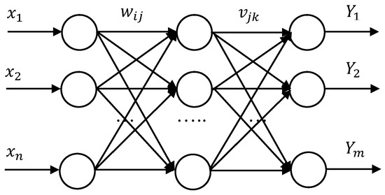
Figure 1.
Three-layer back propagation (BP) neural network structure [24].
The output of the output layer can be expressed as follows [24]:
where and are the weights from the input to the hidden layer and from the hidden to the output layer, respectively, and n, l, and m are the numbers of input, hidden, and output nodes [24].
For each output , error values are formulated by , . s are the actual values for each . The total perturbation then can be obtained as
Output variation with respect to the input variable—i.e., —for and is expressed by
For each output variation due to input perturbation is expressed by the multiplication of weights from the input to the hidden layer and from the hidden to the output layer [24].
2.2. Least Square Error Evaluation
The NN square error value with respect to actual output , , can be expressed as in (4) without consideration of a threshold value [23,24].
The total output error summation is defined as
Equation (5) has the same structure as Equation (2). In the NN model, sensitivity with respect to the input variable is calculated as follows:
From (4) and (6), we obtain
Equation (7) therefore represents the total error with respect to input variation [24]. This shows that the least square error perturbation is obtained by the summation of multiplications between the output error and NN weights. From the relationship between Equations (3) and (7), it is clear that the reliability of the input variables affects the output and error value as highlighted in Section 1. Hence, the previous application of MIV in the selection of reliable data when constructing a simplified NN [24].
3. Reliable Data Generation with ROC
The construction of a NN model is completed when the weights are fixed after the application of training data. Because the performance of a NN model is significantly dependent on the training data used, more training data than available from the real world are often needed to sufficiently train the NN. When real training data are insufficient for NN training, it is necessary to artificially manufacture more training data that can adequately train NN. In this section, we propose a methodology for constructing additional training data using the receiver operating characteristic (ROC) plot [25,26].
3.1. Data Classification with ROC
The ROC has been proposed as a methodology for selecting an appropriate classification threshold leading to the provision of higher quality output information. For example, the ROC plot has been applied to the classification of clinical lab tests since 1950s, where signals or trials are classified based on statistical decision theory [25]. The threshold level for the classification is determined by maximizing true positives and true negatives, which results in the optimum tradeoff between false positives and false negatives [26]. Test and output numbers are illustrated in Table 1.

Table 1.
Number of output and test.
Now we consider the ROC plot of sensitivity with respect to 1–specificity shown in Figure 2; this can also be formed by maximizing the ratio between true positive rate (TPR) and 1–true negative rate (TNR) [28,29]. The output and test results are defined as follows:
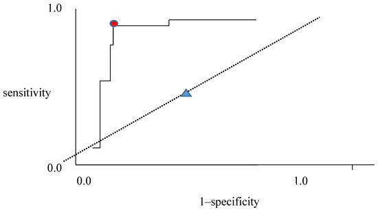
Figure 2.
ROC plot with sensitivity to 1-specificity.
For True Positive(TP): #1; True Negative (TN): #4; False Negative(FN): #3; False Positive (FP): #2
True Positive Rate(TPR):= Sensitivity:
True Negative Rate(TNR):= Specificity:
The ROC plot indicates the division with TP and FP relationship. The red circle close to the top left of Figure 2 illustrates a very good classification. This means that a high likelihood ratio (LR), LR+ = sensitivity/(1–specificity), guarantees more positive than negative outputs when the test is positive. With increasing LR+, we obtain a high TP with an appropriate threshold in the red circle. Similarly, a high LR− = (1–sensitivity)/specificity, guarantees a larger true negative than false negative. The 45-degree dotted line in Figure 2 denotes that no classification happens, it merely serves to divide the data set with half. When data with high temperature, humidity and electricity consumption are chosen, they are considered as conservative and will be selected as true positive in Table 1. Whereas, data with low temperature and electricity consumption belong to true negative in Table 1.
3.2. Generation of Training Data Based on ROC
Here we describe how to generate artificial training data with the help of the ROC plot, which is used to select reliable data components during the generation process. The generation processes are as follows:
- Arrange electricity consumption and input values such as temperature, humidity, and working days for data sets.
- Choose high/low inputs and outputs among successive data sets. Values are TP or TN in Table 2.
Table 2. Output and Test for electricity consumption.
- Generate input and output values.
- Organize training data.
Daily data are considered in Process 1; in this paper, two-day input and output data are considered, successively or randomly. In Process 2, high inputs and outputs are considered to ensure that TP is greater than FP, and low inputs and outputs guarantee TN is greater than FN. Next, we continue to generate input and output data, and gather as training data in Processes 3 and 4, whose further details are illustrated with real data in Section 3.3.
3.3. Illustration of ROC-Based Data Generation with Real Data
To further illustrate the ROC-based training data generation processes, we use actual building electricity consumption data obtained from a shopping mall in Dalian, China [27], which are the same data used to propose the simplified NN with MIV in [24]. In the research, the most effective data were selected from all input data using MIV in order to construct a simplified NN. From the results obtained, it was observed that there were two inputs that significantly affect electricity consumption—i.e., working day and temperature—as summarized in Table 3. Therefore, we compared electricity consumption with all inputs and combinations of inputs through simulation experiments [24]. The importance of sensitivity on the output value was clearly demonstrated [24,30], pointing again to the need for sufficient and reliable training data. From the analysis, we assigned the variable a numeric value {1, 2, 3, 4} = temperature, humidity, working day, weather characteristics. The RMSE for all inputs were found to be 5342.2 kWh, whilst using only {1, 3} resulted in 2291.9 kWh with LM-BP [24].
Table 3.
Mean impact value (MIV) rates (%) for the input factors [24].
In order to generate reliable training data, we considered ROC plots, as discussed in Section 3.2. Electricity consumption data in Appendix A is rearranged by electricity consumption size from largest to smallest as illustrated in Table 4. In the data generation, we generate data by the comparison of k rows. Data generation procedure in this paper, we consider for k = 2 or 3.
Table 4.
Part of training data in Appendix A.
Data generation is carried out based on Table 4 and the generation process are followed by assigning data to make belong to TP and TN based on Table 2; FP and FN data are also generated in the same way.
Firstly, all minimum values from two successive rows of data are selected. For example, the data from 27 April and 8 March, 2014, form the first row of information in Gen_2 below.
- 1)
- Gen_k: Select minimum characteristics per attribute comparing successive days data Table 4 (k = 2)
Process 1 Temperature (°C) Humidity (%) Working Day Weather Characteristics Electricity Consumption (kWh) 04.27/03.08 3 68 0 0.5 15,588 03.08/04.12 3 59 0 0.6 15,145 04.12/04.20 13 40 0 0.8 15,128 - 2)
- Gen_k_cross: Select minimum characteristic per attribute and maximum consumption comparing successive days data Table 4 (k = 2)
Process 2 Temperature (°C) Humidity (%) Working Day Weather Characteristics Electricity Consumption (kWh) 04.27/03.08 3 68 0 0.5 17,385 03.08/04.12 3 59 0 0.6 15,588 04.12/04.20 13 40 0 0.8 15,145
We apply the same procedure to all combinations of two rows.
- 3)
- Gen_k_all: Take all minimum attributes for all combinations of two rows in Table 4 (k = 2)
Process 3 Temperature (°C) Humidity (%) Working Day Weather Characteristics Electricity Consumption (kWh) 04.27/03.08 3 68 0 0.5 15,588 04.27/04.12 13 59 0 0.5 15,145 04.27/04.20 15 40 0 0.5 15,128 - 4)
- Gen_2_all_cross: Take minimum for all characteristics and maximum consumption for all combinations of two rows in Table 4 (k = 2)
Process 4 Temperature (°C) Humidity (%) Working Day Weather Characteristics Electricity Consumption (kWh) 04.27/03.08 3 68 0 0.5 17,385 04.27/04.12 13 59 0 0.5 17,385 04.27/04.20 15 40 0 0.58 17,385 - 5)
- Gen_k_reverse_cross: Select high temperature, humidity, weather characteristics, low working day and high consumption, comparing successive days in Table 4 (k = 2)
Process 5 Temperature (°C) Humidity (%) Working Day Weather Characteristics Electricity Consumption (kWh) 04.27/03.08 15 69 0 0.6 17,385 03.08/04.12 13 69 0 0.9 15,588 04.12/04.20 18 59 0 0.9 15,145
In the process of data generation, 1) and 3) belong to the FT and FN cases, and 2) and 4) belong to the TP and TN data groups. Data generation in 5) is not rational for consideration because high electricity consumption is considered for high temperature and other cases. As described in Section 3.1 and Section 3.2, we generate more reliable data with the help of ROC knowledge: It is expected that the NN model trained with generated data emphasizing TP and TN (i.e., the generation process #2) could provide better predictive performance than the model trained with generated data emphasizing FT and FN, because the former generated data are based on the components providing higher classification performance as shown in Table 2.
4. Illustrative Example and Discussions
In this section, we carry out simulation experiments and compare the prediction performance of a NN model trained with both original data and generated data: We first produce 2/3 of the training data from the original data [27] and compare the prediction results with those with the generated data based on the proposed processes in Section 3, which is followed by the analysis of simulation results and discussions.
4.1. Data Collection or Generation for Training
In the previous section, we generated training data based on the ROC plot. After training with the generated data, testing has been carried out and the results are summarized with root mean square error (RMSE) values in Table 5. From Table 5, it can be seen that the training and test follow a similar pattern.
Table 5.
Training and test results.
The shopping mall covers an area of 50,000 square meters, and thus represents a high-energy consumption building [27]. We use and analyze the building energy consumption data for March and April in 2014. Two-thirds of the calendrical data without generation are used in training for NN, and it shows RMSE with 680.3 kWh. For the training results with Gen_2, Gen_3, Gen_2_cross, and Gen_k_reverse_cross, k = 2, 3 show lower error than the result without generation. For the testing results, Gen_2, Gen_3, and Gen_2_cross and Gen_2_reverse_cross produce lower RMSE than the result without generation as well.
From the numerical results in Table 5, we recognize that training results with generated data show similar phase with the training results. Data generation with Gen_2_all and Gen_2_all_cross is composed with non-successive data pair from electricity consumption viewpoint, so we consider that it is more progressive way of data generation. All the test simulations based on training data are carried out, and the comparisons between each generation procedure from 1) to 5) are illustrated in Figure 3, Figure 4, Figure 5 and Figure 6.
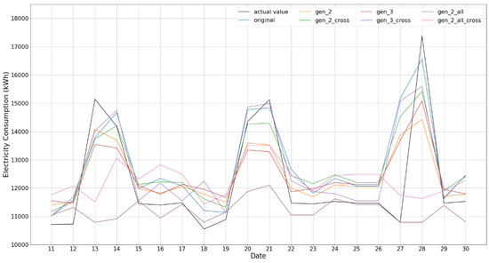
Figure 3.
All test results comparison.
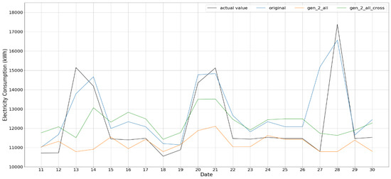
Figure 4.
Gen_2_all and Gen_2_all_cross test result.
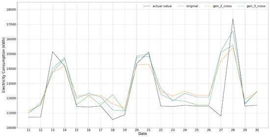
Figure 5.
Gen_k_cross test result for k = 2 and 3.
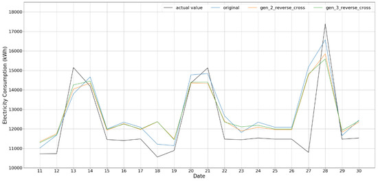
Figure 6.
Gen_k_reverse_cross test result for k = 2 and 3.
The predictions based on generated data, except Gen _2_all and Gen _2_all_cross, provide the test results showing patterns similar to that of the actual value; among them, Gen_k, k = 2, 3, show rather faithful trend in test performance. RMSE of train and test also shows good performance. In case of Gen_2_all and Gen_2_all_cross, as clearly shown in Figure 4, their results are rather flat and could not follow the peak values of the actual value as shown in the figures; as mentioned, this is because the data generation based on the procedure of Gen _2_all does not only consider successive ones only but all combinations, which may not well take into account the time correlation between two consecutive data in time, especially for weather and working day, and, as a result, cannot represent peaks in the original data of building energy consumption.
The results for Gen_k_cross k = 2, 3, shown in Figure 5, which emphasize the data in TP and TN groups, provide rather smaller RMSEs and are faithful in representing peak values. This is also the case for the results for Gen_k_reverse_cross k = 2, 3, shown in Figure 6, which consider data belonging to FT or FN groups. In both the cases, the data generations take into account the time correlation between adjunct rows and, unlike Gen_2_all and Gen_2_all_cross, are able to reproduce well the peaks in the original data of building energy consumption.
4.2. Discussions
As we discussed, the good test performance could be guaranteed from enough training data. Hence, we face with difficulty in training when data are not enough. So, we apply data generation methodology with the help of ROC, and the training process has been done with the part of actual data. Five data generation procedures are introduced and verified by way of simulation.
For the data generation, we find another way of data generation method such as bootstrap application in database [31]. However, the method is carried out in the process by choosing the data with randomly from data set, therefore it cannot be guaranteed that the data is trustworthy. With the obtained result, we can provide more reliable data generation, hence it provides a useful data resource to apply in NN training.
From the simulation results with generated data procedure in Section 3.3, the performance still needs to be improved, even though Gen_k_cross and Gen_k_reverse_cross showed relevant results. Specifically, peak value predictions are not satisfactory and continual difference in low power consumption is illustrated as well. Hence, more diverse considerations are necessary to minimize RMSE and output prediction.
5. Conclusions
A study on the prediction of energy consumption in the building environment has been carried out in this paper. The design of a building model is important to the prediction of the energy consumption and operation scheduling. In NN modelling, the preparation/generation of input training data is the key to its performance and reliability. In our previous work, we used the MIV to screen out insignificant input variables based on the sensitivity analysis and demonstrated its effectiveness [24]. One major issue in the use of MIV, however, is that, because insignificant variables are completely removed during the training data generation and thereby simplified/reduced the structure of NN, all the available information from the original data cannot be fully taken into account in constructing NN.
In order to overcome the issue of data insufficiency in the MIV method, therefore, we generate the training data based on the ROC plot and the statistics of the original data in this work, where boundaries for the selection of input data are decided based on several methods, including successive or combination for two or three data are considered to choose input data. Minimum electric consumption guarantees conservative viewpoint, whereas maximum consumption allows progressive one. We use LM-BP NN structure, which has an advantage in smaller training data. After training data generation, test results are compared with those based on the original (without generation) data.
The experimental results demonstrate that data generation with ROC is more reliable and can overcome the data insufficiency issue of the MIV method, which results in a more efficient and reliable NN model for the prediction of building energy consumption. Specifically, the results with successive data show rather relevant output together with training results. However, two or three data combination case does not follow the consumption phase, that is, a rather conservative prediction; specifically, the results for Gen_2_all and Gen_2_all_cross show a difference of 390~950 kWh and 600~900 kWh for training and test with respect to the reference case of the original data, respectively.
Note that the results from this work can be extend and applied to other research areas, including the construction of NN models with insufficient data set.
Author Contributions
Conceptualization, M.K.K. and V.H.P.; methodology, S.L. and J.C.; software, V.H.P.; validation, K.S.K. and V.H.P.; resources, M.K.K.; writing—review and editing, S.L., K.S.K. and M.L.; supervision, M.K.K. and K.S.K.; funding acquisition, S.L.
Funding
This research was funded by RDF from XJTLU, grant number RDF 14-03-11.
Acknowledgments
The authors appreciate to the support of CeSGIC from XJTLU to finish the research article.
Conflicts of Interest
All authors confirmed that there is no conflict of interest.
Appendix A
Table A1.
Electricity consumption data for a shopping mall in Dalian [27].
Table A1.
Electricity consumption data for a shopping mall in Dalian [27].
| Date | Temperature (°C) | Humidity (%) | Working Day | Weather Characteristics | Electricity Consumption (kWh) | |
|---|---|---|---|---|---|---|
| 04.27 | 15 | 68 | 0 | 0.5 | 17,385 | Sun |
| 03.08 | 3 | 69 | 0 | 0.6 | 15,588 | Sat |
| 04.12 | 13 | 59 | 0 | 0.9 | 15,145 | Sat |
| 04.20 | 18 | 40 | 0 | 0.8 | 15,128 | Sun |
| 04.19 | 17 | 42 | 0 | 0.8 | 14,352 | Sat |
| 04.13 | 16 | 49 | 0 | 0.8 | 14,183 | Sun |
| 03.01 | 5 | 42 | 0 | 0.8 | 13,958 | Sat |
| 04.06 | 18 | 30 | 0 | 1 | 13,868 | Sun |
| 03.22 | 17 | 33 | 0 | 1 | 13,783 | Sat |
| 03.30 | 17 | 31 | 0 | 1 | 13,755 | Sun |
| 03.29 | 14 | 45 | 0 | 0.8 | 13,716 | Sat |
| 03.23 | 16 | 31 | 0 | 1 | 13,701 | Sun |
| 03.15 | 12 | 32 | 0 | 1 | 13,674 | Sat |
| … | .. | .. | . | . | … | … |
| 03.11 | 8 | 42 | 1 | 0.8 | 10,571 | Tue |
| 04.17 | 15 | 76 | 1 | 0.7 | 10,556 | Thu |
| 03.14 | 7 | 31 | 1 | 1 | 9790 | Fri |
| 04.03 | 11 | 31 | 1 | 1 | 9723 | Thu |
| 03.10 | 6 | 30 | 1 | 1 | 9446 | Mon |
| 03.03 | 6 | 46 | 1 | 0.8 | 9148 | Mon |
| 03.12 | 5 | 51 | 1 | 0.9 | 8967 | Wed |
| 03.07 | 4 | 29 | 1 | 1 | 8748 | Fri |
| 03.06 | 5 | 33 | 1 | 1 | 8734 | Thu |
| 03.13 | 4 | 33 | 1 | 1 | 8419 | Thu |
| 03.05 | 3 | 46 | 1 | 1 | 7711 | Wed |
References
- Renewable Energy Policy Network for the 21st Century (REN21). Renewables 2018 Global Status Report. Available online: http://www.ren21.net/gsr-2018/ (accessed on 15 May 2018).
- Administration, N.E. National Energy Administration in China. 2015. Available online: http://www.nea.gov.cn/2016-01/15/c_135013789.htm (accessed on 1 December 2018).
- Xie, Q.; Ouyang, H.; Gao, X. Estimation of electricity demand in the residential buildings of China based on household survey data. Int. J. Hydrogen Energy 2016, 41, 15879–15886. [Google Scholar] [CrossRef]
- Carli, R.; Dotoli, M.; Pellegrino, R.; Ranieri, L. A decision making technique to optimize a building stock energy efficiency. IEEE Trans. Syst. Man Cybern. Syst. 2017, 47, 794–807. [Google Scholar] [CrossRef]
- Pacheco-Torres, R.; Heo, Y.; Choudhary, R. Efficient energy modelling of heterogeneous building portfolios. Sustain. Cities Soc. 2016, 27, 49–64. [Google Scholar] [CrossRef]
- Carli, R.; Dotoli, M.; Pellegrino, R. A Hierarchical Decision Making Strategy for the Energy Management of Smart Cities. IEEE Trans. Autom. Sci. Eng. 2017, 14, 505–523. [Google Scholar] [CrossRef]
- Dall’O’, G.; Norese, M.F.; Galante, A.; Novello, C. A Multi-Criteria Methodology to Support Public Administration Decision Making Concerning Sustainable Energy Action Plans. Energies 2013, 6, 4308–4330. [Google Scholar] [CrossRef]
- Carli, R.; Dotoli, M. Energy scheduling of a smart home under nonlinear pricing. In Proceedings of the 2014 IEEE 53rd Conference on Decision and Control (CDC), Los Angeles, CA, USA, 15–17 December 2014; pp. 5648–5653. [Google Scholar]
- Ahmad, M.W.; Mourshed, M.; Rezgui, Y. Trees vs. Neurons: Comparison between random forest and ANN for high-resolution prediction of building energy consumption. Energy Build. 2017, 147 (Suppl. C), 77–89. [Google Scholar] [CrossRef]
- Ahmad, M.W.; Mourshed, M.; Yuce, B.; Rezgui, Y. Computational intelligence techniques for HVAC systems: A review. Build. Simul. 2016, 9, 359–398. [Google Scholar] [CrossRef]
- Hsu, D. Comparison of integrated clustering methods for accurate and stable prediction of building energy consumption data. Appl. Energy 2015, 160 (Suppl. C), 153–163. [Google Scholar] [CrossRef]
- Shi, G.; Liu, D.; Wei, Q. Energy consumption prediction of office buildings based on echo state networks. Neurocomputing 2016, 216 (Suppl. C), 478–488. [Google Scholar] [CrossRef]
- Tetlow, R.M.; van Dronkelaar, C.; Beaman, C.P.; Elmualim, A.A.; Couling, K. Identifying behavioural predictors of small power electricity consumption in office buildings. Build. Environ. 2015, 92 (Suppl. C), 75–85. [Google Scholar] [CrossRef]
- Ye, Z.; Kim, M.K. Predicting electricity consumption in a building using an optimized backpropagation and Levenberg-Marquardt back-propagation neural network: Case study of a shopping mall in China. Sustain. Cities Soc. 2018, 42, 176–183. [Google Scholar] [CrossRef]
- Neto, A.H.; Fiorelli, F.A.S. Comparison between detailed model simulation and artificial neural network for forecasting building energy consumption. Energy Build. 2008, 40, 2169–2176. [Google Scholar] [CrossRef]
- Doyle, J.C.; Francis, B.A.; Tannembaum, A.R. Feedback Control Theory; Macmillan Publishing Company: London, UK, 1992. [Google Scholar]
- Hashem, S. Sensitivity analysis for feedforward artificial neural networks with differentiable activation functions. In Proceedings of the IJCNN 92, Baltimore, MD, USA, 7–11 June 1992; Volume 1, pp. 419–424. [Google Scholar]
- Fu, L.; Chen, R. Sensitivity analysis for input vector in multilayer feedforward neural network. In Proceedings of the IEEE International Conference Neural Networks, San Francisco, CA, USA, 28 March–1 April 1993; Volume 1, pp. 215–218. [Google Scholar]
- Choi, J.Y.; Choi, C.H. Sensitivity analysis of multilayer perceptron with differentiable activation functions. IEEE Trans. Neural Netw. 1992, 3, 101–107. [Google Scholar] [CrossRef] [PubMed]
- Zeng, X.; Yeung, D.S. Sensitivity analysis of multilayer perceptron to input and weight perturbations. IEEE Trans. Neural Netw. 2001, 12, 1358–1366. [Google Scholar] [CrossRef] [PubMed]
- Stevenson, M.; Winter, R.; Widrow, B. Sensitivity of feedforward neural network to weight error. IEEE Trans. Neural Netw. 1990, 1, 71–80. [Google Scholar] [CrossRef] [PubMed]
- Yeung, D.S.; Sun, X. Using function approximation to analyze the sensitivity of MLP with antisymmetric squashing activation function. IEEE Trans. Neural Netw. 2002, 13, 34–44. [Google Scholar] [CrossRef] [PubMed]
- Zhang, Z.; Jin, X. Prediction of peak velocity of blasting vibration based on artificial Neural Network optimized by dimensionality reduction of FA-MIV. Math. Probl. Eng. 2018, 2018, 8473547. [Google Scholar] [CrossRef]
- Kim, M.K.; Cha, J.; Lee, E.; van Pham, H.; Lee, S.; Theera-Umpon, N. Simplified Neural Network Model Design with Sensitivity Analysis and Electricity Consumption Prediction in a Commercial Building. Energies 2019, 12, 1201. [Google Scholar] [CrossRef]
- Zweig, M.H.; Campbell, G. Receiver Operating Characteristic (ROC) Plots: A fundamental evaluation tool in clinical medicine. Clin. Chem. 1993, 39, 561–577. [Google Scholar]
- Bewick, V.; Cheek, L.; Ball, J. Statistics review 13: Receiver operating characteristic curves. Crit. Care 2004, 8, 508–512. [Google Scholar] [CrossRef]
- Liu, Z.P. Research and Design of Wireless Monitoring System for Building Energy Consumption. Master’s Thesis, Dalian University of Technology, Dalian, China, 2015. (In Chinese). [Google Scholar]
- Altun, K.; Barshan, B. Human activity recognition using inertial/magnetic sensor units. In Lecture Notes in Computer Science, Proceedings of the International Workshop on Human Behavior Understanding, Istanbul, Turkey, 22 August 2010; Springer: Berlin/Heidelberg, Germany, 2010; pp. 38–51. [Google Scholar]
- Geng, Y.; Chen, J.; Fu, R.; Bao, G.; Pahlavan, K. Enlighten wearable physiological monitoring systems: On-body RF characteristics based human motion classification using a support vector machine. IEEE Trans. Mob. Comput. 2016, 15, 656–671. [Google Scholar] [CrossRef]
- Saltelli, A.; Tarantola, S.; Campolongo, F. Sensitivity analysis as an ingredient of modelling. Stat. Sci. 2000, 15, 377–395. [Google Scholar]
- Bellec, P.; Perlbarg, V.; Evans, A.C. Bootstrap generation and evaluation of an fMRI simulation database. Magn. Reson. Imaging 2009, 27, 1382–1396. [Google Scholar] [CrossRef] [PubMed]
© 2019 by the authors. Licensee MDPI, Basel, Switzerland. This article is an open access article distributed under the terms and conditions of the Creative Commons Attribution (CC BY) license (http://creativecommons.org/licenses/by/4.0/).