Sustainable Synthesis Processes for Carbon Dots through Response Surface Methodology and Artificial Neural Network

Abstract

Nowadays, to ensure sustainability of smart materials, it is imperative to eliminate or reduce carbon footprint related to nano material production. The concept of design of experiment to provide an optimal synthesis process, with a desired yield, is indispensable. It is the researcher’s goal to get optimum value for experiments that requires multiple runs and multiple inputs. Herein, is a reliable approach of utilizing design of experiment (DOE) for response surface methodology (RSM). Thus, to optimize a facile and effective synthesis process for fluorescent carbon dots (CDs) derived from tapioca that is in line with green chemistry principles for sustainable synthesis. The predictions for fluorescent CDs synthesis from RSM were in excellent agreement with the artificial neural network (ANN) model prediction by the Levenberg–Marquardt back propagation (LMBP) algorithm. Considering R², root mean square error (RMSE) and mean absolute error (MAE) have all revealed a positive hidden layer size. The best hidden layer of neurons were discovered at point 4-8, to confirm the validity of carbon dots, characterization of surface morphology and particles sizes of CDs were conducted with favorable confirmations of the unique characteristics and attributes of synthesized CDs by hydrothermal route.

1. Introduction

The process of optimizing synthesis parameters (factors) to provide high quality organic carbon dots (CDs) represents a complex process. It is a similitude of a search in the dark. Several researchers have reported a low value of photoluminescence, long hours synthesis, and high volume of resources used in the process of CDs [1,2]. Attempting to synthesize CDs needs optimization by an appropriate mathematical model, which is embedded with the task to optimize the synthesis process in terms of quality criteria and prediction with less error. This is necessary due to the influence of factors that may or may not affect the quality of yield. So far, the synthesis of sustainable organic CDs with high performance yield is still being researched. In the past, synthesis processes that involved multiple factors were conducted by varying a single factor while others were kept constant, known as one variable at a time (OVAT), but this method is time consuming. It became imperative to formulate multivariate statistics that substantially reduce the numbers of experiments [3].

Nwobi-Okoye and Ochieze [4] made a study based on the comparison of Response Surface Methodology (RSM) and Artificial Neural Network (ANN) data to validate the prediction of aluminum alloy A356/cow horn particulate composites hardness. The study confirmed that ANN with R² of 0.9921 exhibited better accuracy than the RSM with R² of 0.9583 in predicting the hardness values of the composites [4]. The ANN model is generally based upon artificial intelligence (machine learning), under which a predefined set of data is being trained [5,6], validated, and tested for prediction purposes. Due to this constraint, it is worthy to note that the values predicted by ANN will not often be the best predicted values, but will be within the range of the experimental study [7,8].

RSM is a technique that has been widely applied for defining the interactions between various process parameters and responses with the various desired criteria and taking note of the significance of these process parameters on the desired responses [9]. However, RSM is reported not to be desirable to optimize the non-linear system study that possesses minimal difference in parts, processing boundaries, or investigated data sets because it affects the overall properties of material [9]. The prediction of RSM is based on a first or second order polynomial equation, hence, it is inadequate enough to capture non-linear behavior and can give a non-reliable estimation of photoluminescent quantum yield of fluorescent carbon dots of organic origin. Consequently, the application of the artificial neural network (ANN) can be employed to checkmate and surmount concerns of using a lone RSM in predicting the non-linear system. The concept of ANN is an independent method that uses a model that effectively handles nonlinearity in responses that concerns the synthesis and photoluminescent quantum yield of carbon dots.

Formulating an ANN model which accepts a small data set of experimental runs while supplying a useful output in the synthesis of an advanced nanoparticle (CDs) is studied here. From the studies conducted, there are no results published by using the Levenberg–Marquardt back propagation (LMBP) algorithm in the synthesis of fluorescent carbon dots from tapioca powder. With this in view, the LMBP training algorithm was built and deployed in the current study to predict the photoluminescent quantum yield of the synthesized carbon dots from tapioca powder.

In this report, sample data were acquired from design of experiment for response surface methodology (RSM). The training and predictions by an artificial neural network (ANN) were carried out by different multi inputs, and multi output ANN, developed using the Levenberg–Marquardt back propagation (LMBP) algorithm to predict the fluorescent properties of carbon dots synthesized in the study.

2. Mathematical Models and Analytical Methods

2.1. Response Surface Method and Mathematical Model

The design software utilized was Design-Expert Version 11.0.5. Central composite design (CCD) was adopted for the analysis of effects. These consist of four (4) independent variables: Temperature (X1), Dosage (X2), Time (X3), and W/Ace/NaOH ratio (X4), as shown in

Table 1. Independent variables used in the Response Surface Methodology (RSM) design.

Factor	Name	Units	Low Actual	High Actual	Low Coded	High Coded	Mean	Std. Dev.
A (X1)	Temp	°C	75.00	175.00	−1.000	1.000	125.0	40.825
B (X2)	Dosage	g	0.100	0.50	−1.000	1.000	0.30	0.163
C (X3)	Time	min	45.00	105.00	−1.000	1.000	75.00	24.495
D (X4)	W/Ace/NaOH	mL	8.00	40.00	−1.000	1.000	24.00	13.064

below. A total sum of 30 experimental runs were carried out, photoluminescent quantum yield (PLQY) was the response considered and expressed as the dependent variable shown in

Table 2. Design of experiment for response surface methodology report.

Std Order	Factor-A Temperature (°C)	Factor-B Dossage (gram)	Factor-C Time (min)	Factor-D Solvent (mL) (H2O/C3H6O/NaOH)	Exp. Actual Value (PLQY)	Pred. Value	Res. Value
1	75	0.10	45	8.00	14.67	14.41	0.26
2	175	0.10	45	8.00	21.05	20.89	0.15
3	75	0.50	45	8.00	22.80	22.35	0.45
4	175	0.50	45	8.00	19.96	19.13	0.83
5	75	0.10	105	8.00	14.00	13.01	0.99
6	175	0.10	105	8.00	25.27	26.13	−0.86
7	75	0.50	105	8.00	20.15	21.52	−1.36
8	175	0.50	105	8.00	24.87	24.94	−0.06
9	75	0.10	45	40.00	24.82	24.39	0.42
10	175	0.10	45	40.00	20.99	19.88	1.11
11	170	0.1	100	12.00	27.75	27.38	0.37
12	175	0.50	45	40.00	12.53	13.16	−0.63
13	75	0.10	105	40.00	17.90	18.99	−1.09
14	175	0.10	105	40.00	21.04	21.13	−0.09
15	75	0.50	105	40.00	22.75	22.55	0.21
16	175	0.50	105	40.00	14.46	14.98	−0.51
17	54	0.30	75	24.00	24.28	24.57	−0.30
18	195	0.30	75	24.00	23.89	23.80	0.08
19	125	0.02	75	24.00	24.49	25.08	−0.59
20	125	0.58	75	24.00	26.73	26.35	0.38
21	125	0.30	32	24.00	18.53	20.74	−2.22
22	125	0.30	117	24.00	23.04	21.03	2.01
23	125	0.30	75	1.37	16.74	16.98	−0.24
24	125	0.30	75	46.63	17.02	16.99	0.03
25	125	0.30	75	24.00	23.53	23.58	−0.05
26	125	0.30	75	24.00	24.53	23.58	0.94
27	125	0.30	75	24.00	22.89	23.58	−0.69
28	125	0.30	75	24.00	22.53	23.58	−1.06
29	125	0.30	75	24.00	23.93	23.58	0.34
30	125	0.30	75	24.00	24.53	23.58	0.94

Predicted Value = Pred. value, Res. Value = Residual value. Study Type: Response Surface, Runs: 30, Initial Design: Central Composite, Design Model: Quadratic.

. The inputs variables were expressed individually as a function of independent variables. A second-order polynomial equation was used to express PLQY (Y1) as an independent variable. Given in the equation below:

$$Y={\beta }_0+{\displaystyle \sum }_{i=1}^4{\beta }_i{X}_i+{\displaystyle \sum }_{i=1}^4{\beta }_{ii}{X}_i^2+{\displaystyle \sum }_{i<j}^4{\beta }_{ij}{X}_i{X}_j$$

(1)

where, Y represents the response variable, ${\beta }_0$ is a constant, ${\beta }_i$, ${\beta }_{ii}$, and ${\beta }_{ij}$ are the linear, quadratic, and cross-product coefficients, respectively. Xi and Xj are the respective levels of the independent variables. Three dimensional (3D) surface response plots were generated by varying two variables at a time within the experimental range and holding the other two constant at the central point. Furthermore, a test of statistical significance was based on the total error criteria with a confidence level of 95.0%. Below is the response surface methodology (RSM) design summary.

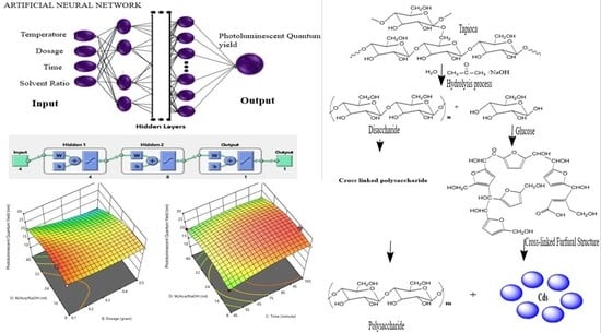
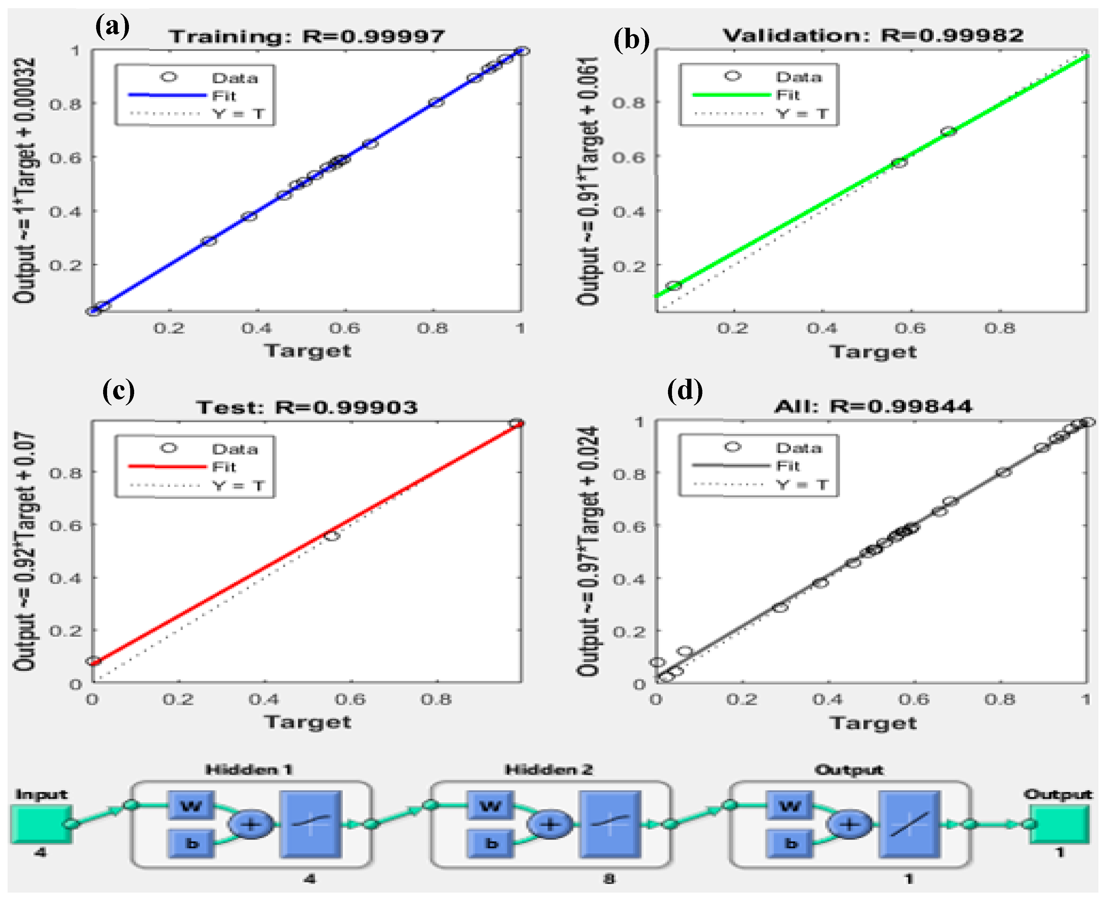
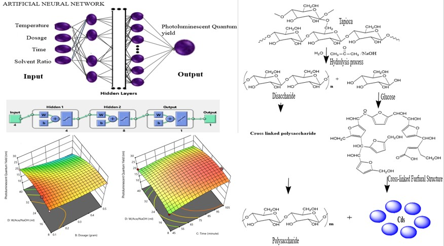
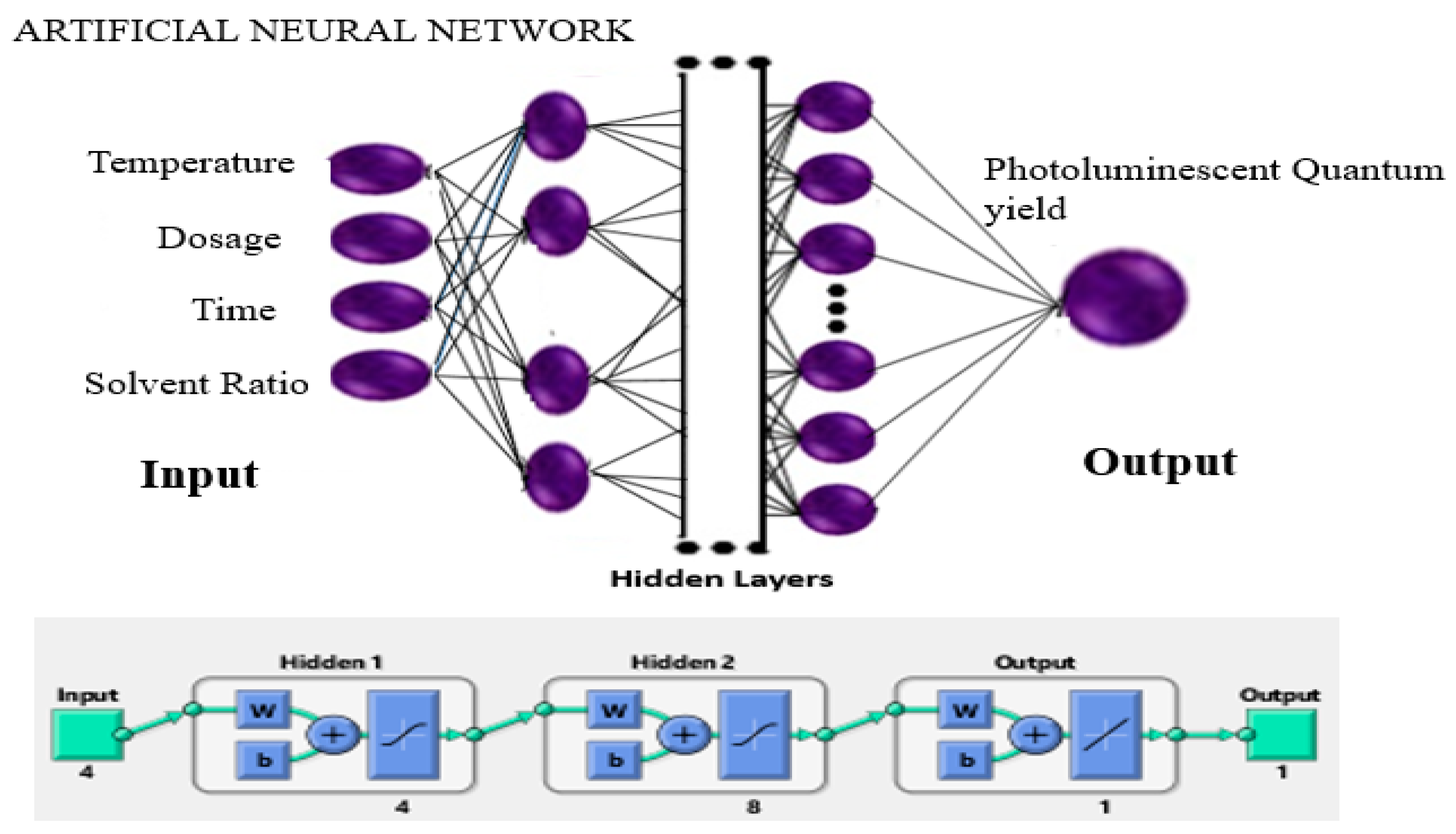
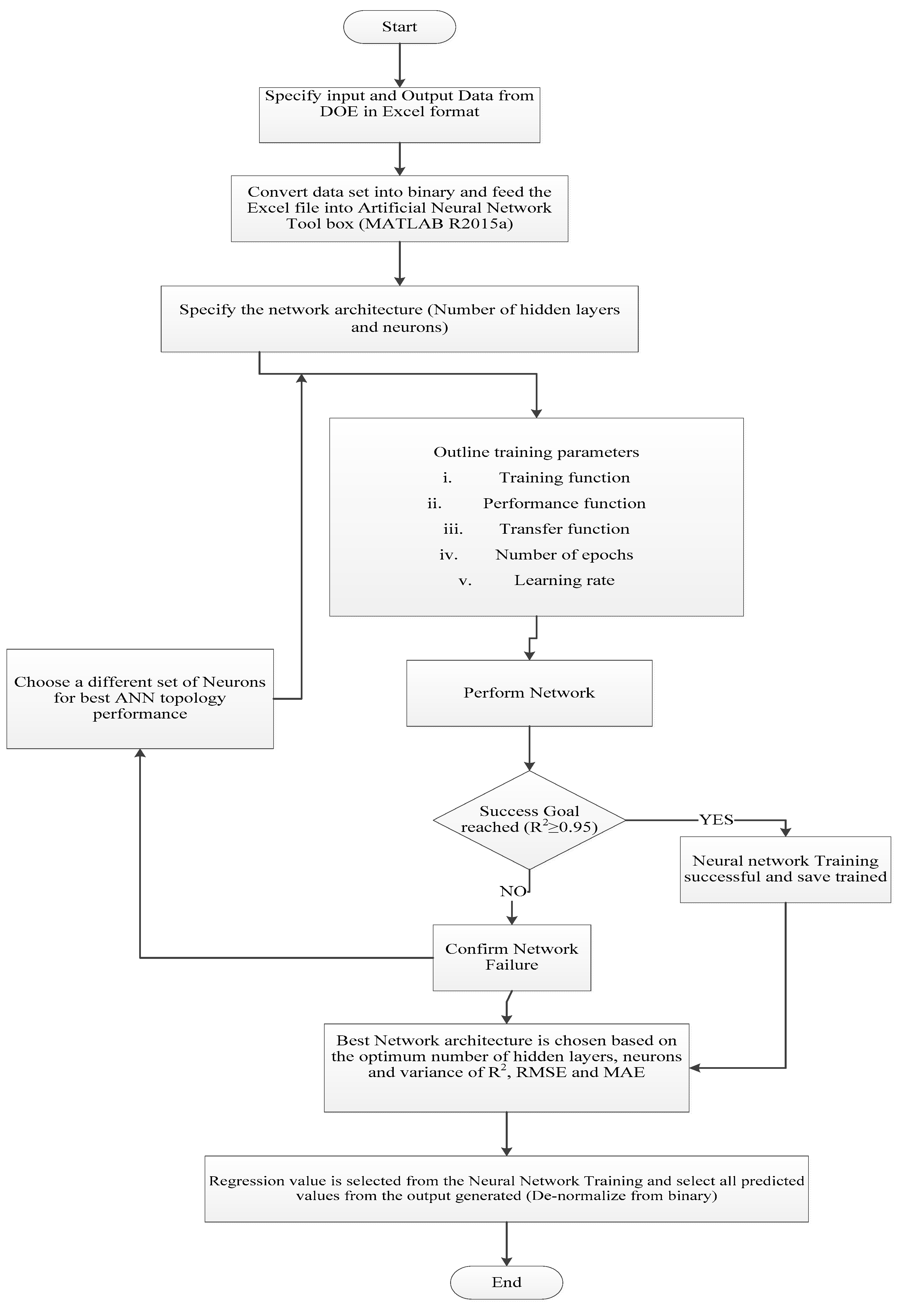
2.2. Artificial Neural Network Mathematical Model and Method

Response surface methodology data along with the experimental data was collected from sample formulation, totaling 30 samples. These sample data were used in the training of overall data. Note; the regular data collected where normalized to a range between 0 and 1 using Equation (2) below.

$$X_{norm}=\frac{X-X_{min.}}{X_{\max -X_{min}}}$$

(2)

The X_norm is the normalized value, X is the variable, X_min and X_max are the minimum and maximum values among the data set.

The normalization is necessary to execute the sigmoid transfer function effectively. The network model was programmed by codes of multilayer perceptron (MLP) along with the training algorithm of back propagation (BP), which consists of an input layer (the input variables of temperature, time, dosage, and solvent ratio), a hidden layer and an output layer (photoluminescent quantum yield) which was the response generated from the experimental values. These three node layers are neurons that utilizes non-linear activation function as given in Figure 1 below.

Data tests have shown that a pair of hidden layer resulted in a high performance value. Thus, after multiple iterations for the best data set performance, artificial neural network topologies were selected based on the log-sigmoid transfer function (Equation (3)), linear transfer function in the output layer (Equation (4)), and best performance criteria of coefficient of determination (R²) at Equation (5), mean absolute error (MAE) at Equation (6), and root mean square error (RMSE) at Equation (7).

$$Logsig \left(n\right)=\frac{1}{1+exp\left(-n\right)}$$

(3)

$$Pureline \left(n\right)=n$$

(4)

$$R^2=1-{\displaystyle \sum }_{i=1}^n\left[\frac{{(y_{pred}^i -y_{targ}^i)}^2}{{(y_{avg,targ}-y_{targ}^i)}^2}\right]$$

(5)

$$MAE=\frac{1}{N}{\displaystyle \sum }_{i=1}^N\left|y_{pred}^i-y_{targ}^i\right|$$

(6)

$$RMSE=\sqrt{{\displaystyle \sum }_{i=1}^N\frac{{(y_{Pred}^i-y_{targ}^i)}^2}{N}}$$

(7)

where, n is the number of experimental data, $y_{Pred}^i$ is the predicted value and $y_{targ}^i$ is real value obtained from experimental data, $y_{avg,targ}$ is the average experimental value. However, the value of R² is the amount of reduction in the variability of the response by using a repressor variable in the model. R² close to 1 is desirable and the root mean square error (RMSE) is required to be negligibly infinitesimal [10].

The process of developing an artificial intelligence model for the prediction and optimization of fluorescent carbon dots followed the flow chart in Figure 2. The chart demonstrates the procedural flow involved in the formulation of the artificial neural network for photoluminescent quantum yield prediction and optimization for the synthesized fluorescent carbon dots (see Section 2.3 for synthesis approach).

A multi input and a single output artificial neural network model was developed by utilizing the Levenberg–Marquardt back propagation (LMBP) algorithm to effectively predict the photoluminescent quantum yield of synthesized fluorescent carbon dots [11,12].

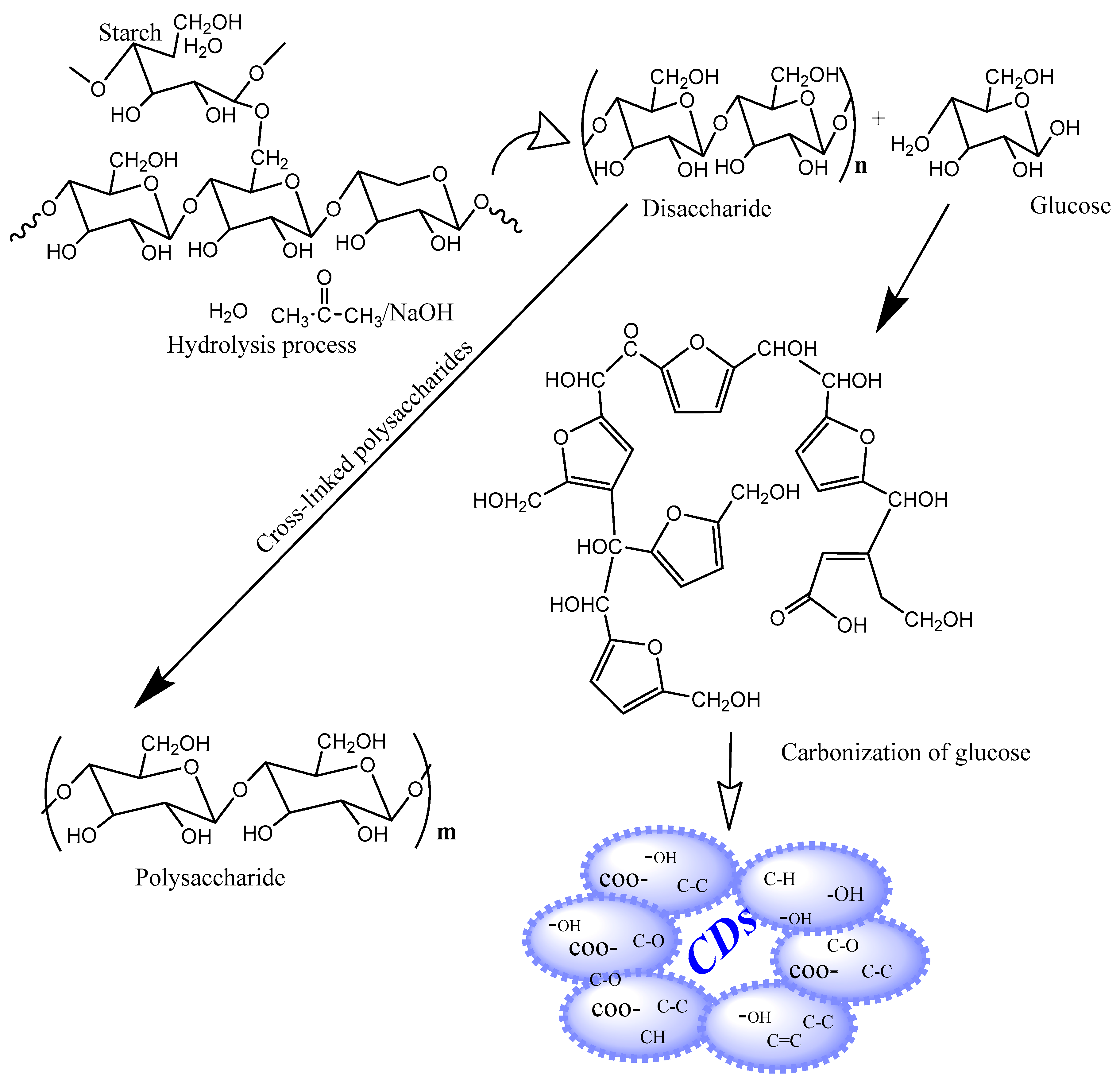
2.3. Synthesis of Carbon Dots (CDs)

An environmental suitable technique for producing carbon dots, (hydrothermal synthesis process), were adopted from the response surface methodology analysis. The best photoluminescent quantum yield data were used here for the report of the response. A small quantity, (0.1 g), of tapioca flour was mixed in 12 mL prepared solvent ratio (deionized water + sodium hydroxide + acetone), see Figure 3 for mechanism flow. This mixture was placed in a stainless steel hydrothermal reactor in a convection oven at a temperature of 170 °C for a period of 1 h 40 min. This study has successfully reduced the needed temperature and time needed for synthesizing CDs [13,14,15].

The mixture was centrifuged for 20 min at 3000 rpm. For clarity (no substantial suspended solids detected). The photoluminescent quantum yield was thus calculated by;

$$Q=Q_R(\frac{GRAD}{GRA{D}_R})(\frac{{ἠ}^2}{{ἠ}_R^2})$$

(8)

3. Result and Discussion

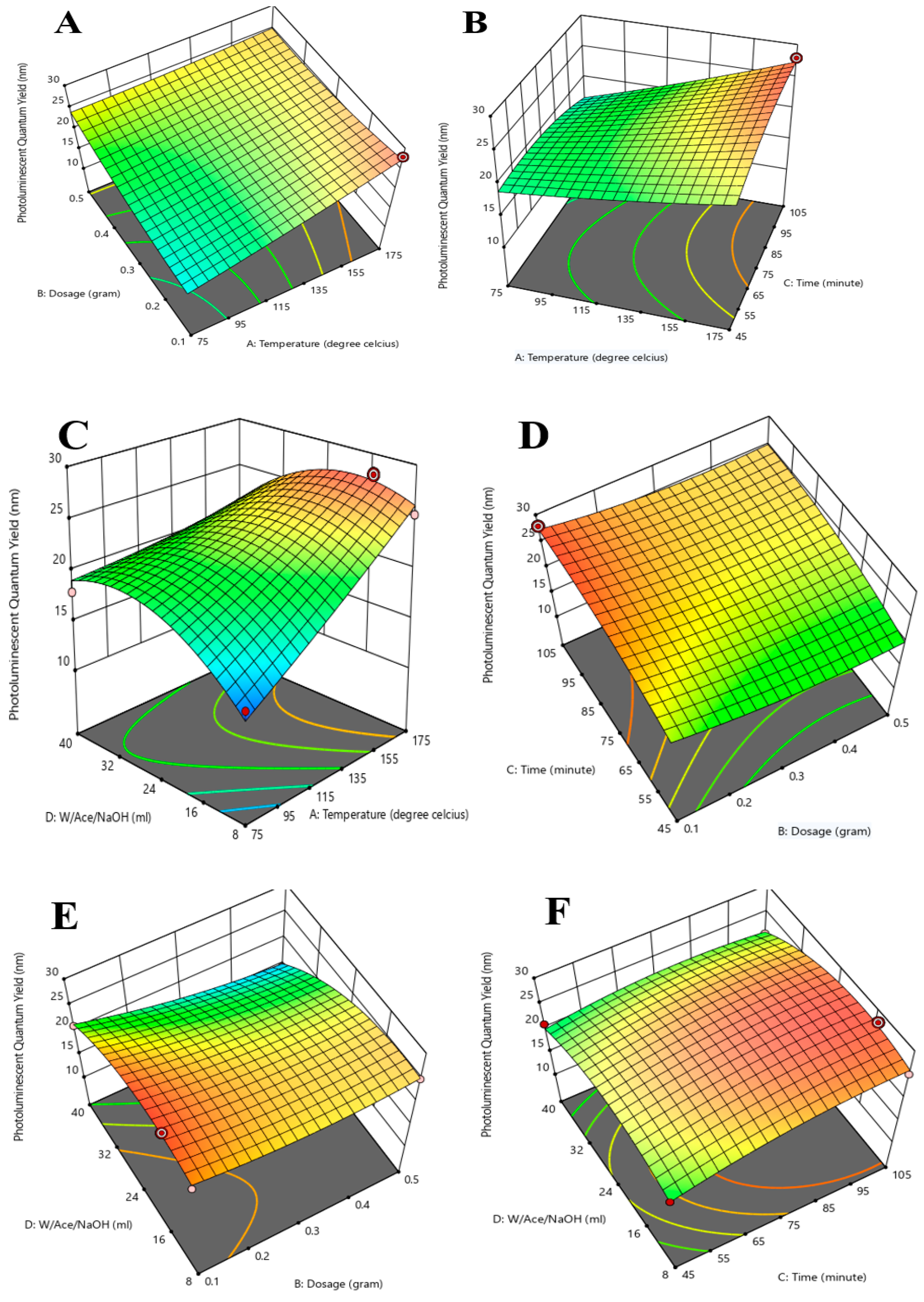
3.1. Response Surface Methodology

The design of experiment data (ref: Table 1) was used as independent variables inputs. The best outputs of photoluminescent quantum yield (PLQY) of carbon dots, the predicted and actual experimental values of photoluminescent quantum yield, is reported in Table 2 below.

It shows a positive model with an R² value of 0.956 as revealed on the fits statistics (Table 6), a high experimental value of PLQY of 27.75%, and a predicted value of 27.38% with a residual value of 0.37%. The experimental data was then used to calculate the coefficient of polynomial equation for the response yield with the inputs data of temperature, time, dosage, and solvent ratio; by adopting Equation (1).

The results of design of experiment was computed by central composite design (CCD) as stated earlier. Photoluminescent quantum yield of the predicted and experimental yield was given by a model equation as in Equation (1) and represented by the expression below.

• A = temperature, B = dosages, C = time, D = solvent (H₂O/C₃H₆O/NaOH)
• Now, let;
• A = X₁, B = X₂, C = X₃, D = X₄ (refer to RSM Table 2)

i

Final equation in terms of coded (predicted) factors (full model): Also see

Table 3. The fitted quadratic model in terms of coded variables.

Response	2nd Order Polynomial Equation	Regression (p-Value)	R2	R2 (Adjusted)	Lack of Fit
PLQY	23.63 − 0.1732 X1 + 0.03498 X2 + 0.1905 X3 −0.0802 X4 − 2.38 X1 X2 + 1.61 X1 X3 − 2.68 X1 X4 + 0.1894 X2 X3 − 1.30 X2 X4 – 0.9353 X3 X4 + 0.2905 X21 + 1.07 X22 − 1.38 X23 − 3.36 X24.	0.0001	0.9563	0.9155	0.1685

below for R² values and lack of fit for the polynomial regression equation.

Photoluminescent quantum yield (Response) = 23.63 − 0.1732 X₁ + 0.03498 X₂ +
0.1905 X₃ − 0.0802 X₄ − 2.38 X₁ X₂ + 1.61 X₁ X₃ − 2.68 X₁ X₄ + 0.1894 X₂ X₃ − 1.30 X₂ X₄ −
0.9353 X₃ X₄ + 0.2905 X²₁ + 1.07 X²₂ − 1.38 X²₃ − 3.36 X²₄.

ii

Final equation in terms of actual factors (full model): Also see

Table 4. The fitted quadratic model in terms of actual variables.

Response	2nd Order Polynomial Equation	Regression (p-Value)	R2	R2 (Adjusted)	Lack of Fit
PLQY	−3.3822 + 0.03866 X1 + 22.7576 X2 + 0.1385 X3 + 1.3133 X4 − 0.2379 X1 X2 + 0.0010 X1 X3 − 0.0033 X1 X4 + 0.0315 X2 X3 − 0.4069 X2 X4 − 0.0019 X3 X4 + 0.0001 X21 + 26.8733 X22 − 0.0015 X23 − 0.0131 X24.	0.0001	0.9563	0.9155	0.1685

below for R² values and lack of fit for the polynomial regression equation.

Photoluminescent quantum yield (Response) = −3.3822 + 0.03866 X₁ + 22.7576 X₂ +
0.1385 X₃ + 1.3133 X₄ − 0.2379 X₁ X₂ + 0.0010 X₁ X₃ − 0.0033 X₁ X₄ + 0.0315 X₂ X₃ −
0.4069 X₂ X₄ − 0.0019 X₃ X₄ + 0.0001 X²₁ + 26.8733 X²₂ − 0.0015 X²₃ − 0.0131 X²₄.

Analysis of Variance and Model Statistical Report

The data set for the response surface methodology as generated by the software made the model to fit in to quadratic significance, and the analysis of variance (ANOVA) for statistical significance of the quadratic model is computed on

Table 5. ANOVA for quadratic model.

Source	Sum of Squares	df	Mean Square	F-Value	p-Value
Model	446.88	14	31.92	23.45	<0.0001	significant
A-Temperature	0.5324	1	0.5324	0.3912	0.5411
B-Dosage	2.14	1	2.14	1.57	0.2289
C-Time	0.6458	1	0.6458	0.4745	0.5014
D-W/Ace/NaOH	0.1132	1	0.1132	0.0832	0.7770
AB	83.27	1	83.27	61.18	<0.0001
AC	38.33	1	38.33	28.16	<0.0001
AD	101.98	1	101.98	74.93	<0.0001
BC	0.5274	1	0.5274	0.3875	0.5430
BD	24.01	1	24.01	17.64	0.0008
CD	12.38	1	12.38	9.10	0.0087
A2	0.7806	1	0.7806	0.5735	0.4606
B2	10.48	1	10.48	7.70	0.0142
C2	17.76	1	17.76	13.05	0.0026
D2	106.01	1	106.01	77.89	<0.0001
Residual	20.42	15	1.36
Lack of Fit	16.94	10	1.69	2.44	0.1685	Not significant
Pure Error	3.47	5	0.6947
Cor Total	467.30	29

below;

F-value of 23.45 implies the model is significant and the subsequent values for the parameters show their degree of effects on the response of photoluminescent quantum yield for fluorescent carbon dots. Herewith, in Table 5, the most effective single–multiple parameter is the solvent ratio (D²) with an F-value of 77.89. While, interactive most effective parameters are temperature and solvent ratio (AD) with F-value 74.93. The least effective single parameter is temperature (A²) with an F-value of 0.5735 and the least effective interactive parameters are dosage and time (BC) with an F-value of 0.3875 [16,17].

Model p-values less than 0.0500 indicate the model terms are significant [18]. In this case AB, AC, AD, BD, CD, B², C², D² are significant model terms. Values greater than 0.1000 indicate the model terms are not significant, hence, individual lone factors are independent and are non-effective. Favorable interactive effects were observed between temperature and dosage (AB), temperature and time (AC), temperature and solvent (AD), dosage and solvent ratio (BD), and time and solvent ratio (CD), while the individual factor effects were observed with dosage (D²), time (C²), and solvent ratio (D²). Non favorable interactive effects were observed with dosage and time (BC), and the multiple factor of non-effect is temperature (A²). If there are many insignificant model terms (not counting those required to support hierarchy), model reduction may be considered to improve the model, however, in this study the non-effects are few and infinitesimal. The lack of fit F-value of 2.44 implies the lack of fit is not significant relative to the pure error. Non-significant lack of fit is an excellent requirement, since it is needed for the model to fit [19].

The experimental R² of 0.9563 in

Table 6. Fit statistics summary.

Std. Dev.	1.17	R²	0.9563
Mean	21.40	Adjusted R²	0.9155
C.V. %	5.45	Predicted R²	0.7689
		Adequate Precision	17.5186

, shows a significant response [20]. The predicted R² of 0.7689 is in reasonable agreement with the adjusted R² of 0.9155; i.e., the difference is less than 0.2 [21]. Adequate precision, measures the signal to noise ratio, thus, ratio greater than 4 is desirable. Ratio of 17.519 indicates an adequate signal.

This model is significant to navigate the design space. It is necessary for a model to comply with the following;

i

A significant model: Large F-value with p < 0.05.

ii

Insignificant lack-of-fit: F-value with p > 0.10.

iii

Adequate precision >4 [18,19,20].

Furthermore, from Figure 4 below, the three dimensional (3D) plots have shown interactive responses to the favorable yield of photoluminescent quantum yield at 27.75% and the intercept value of 23.63 on the 2nd order polynomial equation of actual values is suitable.

In Figure 4A the interactive behavior of temperature (A) at 170 °C and dosage (B) at 0.1 g has an effective interaction with an F-value of 61.18 and a p-value less than 0.0001 with a value of −0.2379 in the 2nd order polynomial equation of actual factors. Figure 4B is an interactive effect of temperature (A) and time (C) at 1 h 40 min. It records a linear effect on the response value of photoluminescent quantum yield with a favorable p-value that is less than 0.001 and a coefficient value of 1.6143 on the polynomial equation. The interactive effect of temperature (A) and solvent ratio W/Ace/NaOH (D) at 12 mL have the best effect on the response yield of photoluminescent quantum yield with an f-value of 74.93 and a p-value less than 0.0001, coefficient of −2.68 as seen in the 2nd order polynomial equation with a linear response as shown in Figure 4C.

Figure 4D shows a non-effective interaction between dosage (B) and time (C) on the response of photoluminescent quantum yield. p-value at 0.5430 and f-value of 0.3875 all fall short of the requirement of a p-value <0.100 and an f-value that is extremely low. The interactive effect of dosage (B) and solvent ratio W/Ace/NaOH (D) at p-value 0.0008 as shown in the 3D plot on Figure 4A,C,E,F is the most important factor in the sustainability of environmental resources. Environmental resources management is an essential factor to be considered in the synthesis of products, with high emphasis on minimal resource requirement [18].

3.2. Photoluminescent Quantum Yield

The photoluminescent quantum yield (PLQY) of the CDs was ascertained by Equation (8) as in Section 2.3. Using quinine sulfate added to H₂SO₄ to form 0.1 M solution, optical density of 0.00, 0.02, 0.04, 0.06, 0.08, 0.1 were obtained; at absorption wavelength of 340 nm and dilution was made from the synthesized carbon dots solution. The procedure, is an established process of calculating quantum yields of photoluminescent substances. Quinine sulphate as reference quantum yield was held at 54.6 [22,23,24,25,26].

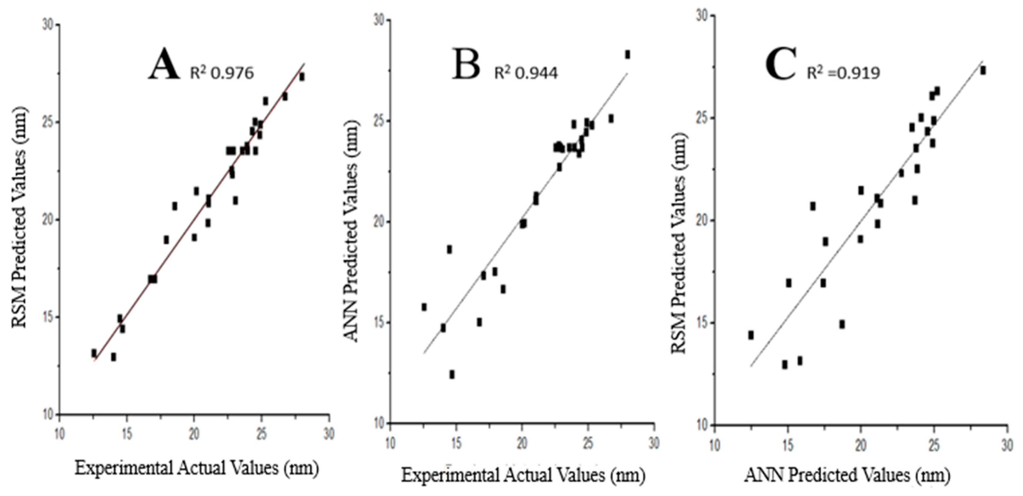
3.3. Evaluation Performance between Artificial Neural Network (ANN) and Response Surface Methodology (RSM) on the Yield of Photoluminescent Quantum Yield

Artificial neural Network (ANN) is a system that mimics the naturally inspired computational model. Thus, it emulates the workings of the human brain to take in certain connections among information inputs and yield outputs through trained data [27,28,29,30].

From

Table 7. Response surface methodology and artificial neural network.

Std Order	Factor-A Temperature (°C)	Factor-B Dossage (gram)	Factor-C Time (min)	Factor-D Solvent (mL) (H2O/C3H6O/NaOH)	Exp. Actual Value (PLQY%)	RSM Pred. Value	ANN. Pred. Value
1	75	0.10	45	8.00	14.67	14.41	12.46
2	175	0.10	45	8.00	21.05	20.89	21.31
3	75	0.50	45	8.00	22.80	22.35	22.74
4	175	0.50	45	8.00	19.96	19.13	19.93
5	75	0.10	105	8.00	14.00	13.01	14.76
6	175	0.10	105	8.00	25.27	26.13	24.84
7	75	0.50	105	8.00	20.15	21.52	19.99
8	175	0.50	105	8.00	24.87	24.94	24.96
9	75	0.10	45	40.00	24.82	24.39	24.51
10	175	0.10	45	40.00	20.99	19.88	21.10
11	170	0.1	100	12.00	27.75	27.38	26.25
12	175	0.50	45	40.00	12.53	13.16	15.80
13	75	0.10	105	40.00	17.90	18.99	17.56
14	175	0.10	105	40.00	21.04	21.13	21.07
15	75	0.50	105	40.00	22.75	22.55	23.82
16	175	0.50	105	40.00	14.46	14.98	18.69
17	54	0.30	75	24.00	24.28	24.57	23.45
18	195	0.30	75	24.00	23.89	23.80	24.89
19	125	0.02	75	24.00	24.49	25.08	24.09
20	125	0.58	75	24.00	26.73	26.35	25.17
21	125	0.30	32	24.00	18.53	20.74	16.69
22	125	0.30	117	24.00	23.04	21.03	23.65
23	125	0.30	75	1.37	16.74	16.98	15.06
24	125	0.30	75	46.63	17.02	16.99	17.38
25	125	0.30	75	24.00	23.53	23.58	23.72
26	125	0.30	75	24.00	24.53	23.58	23.72
27	125	0.30	75	24.00	22.89	23.58	23.72
28	125	0.30	75	24.00	22.53	23.58	23.72
29	125	0.30	75	24.00	23.93	23.58	23.72
30	125	0.30	75	24.00	24.53	23.58	23.72

Predicted Value = Pred. value, Study Type: Response Surface, Runs: 30, Initial Design: Central Composite, Design Model: Quadratic.

below, it shows the relationship between the response surface methodology and the artificial neural network performance of the trained data (see Figure 5). The best output for photoluminescent quantum yield was obtained at No. 11 at actual experimental value of 27.75%, RSM predicted value of 27.38%, and ANN predicted value of 26.25%. The training of the data set was conducted by Matlab R2015a (8.5.0.197613), utilizing Lavenberg–Marquardt algorithm (LMA). The LMA is based on the training neural network through iteration and reiteration of data set weight and bias values as shown on

Table 8. Artificial neural network (ANN) optimum values for hidden layer sizes and corresponding transfer functions (‘tansig’ and ‘logsig’) for minimum error fittings for train, validation, and test of optimized RSM data.

Hidden Neurons	Train			Validation			Test			All
	R2	RMSE	MAE	R2	RMSE	MAE	R2	RMSE	MAE	R2
4-8 *	0.99	0.09	0.06	0.99	0.07	0.04	0.99	0.08	0.06	0.99
8-4	0.99	0.03	0.01	0.95	0.10	0.09	0.95	0.11	0.09	0.94
8-16	0.99	0.04	0.03	0.78	0.17	0.13	0.96	0.12	0.09	0.93
9-19	0.99	0.02	0.01	0.93	0.13	0.08	0.99	0.11	0.09	0.96
11-4	0.99	0.04	0.03	0.85	0.11	0.09	0.95	0.14	0.11	0.96
11-7	0.99	0.02	0.01	0.97	0.07	0.06	0.82	0.12	0.09	0.97
11-9	0.99	0.02	0.01	0.99	0.11	0.09	0.83	0.15	0.12	0.96
13-9	0.95	0.07	0.05	0.92	0.14	0.13	0.94	0.12	0.09	0.93
13-13	0.99	0.03	0.02	0.76	0.11	0.09	0.93	0.16	0.13	0.95
17-10	0.99	0.02	0.01	0.90	0.12	0.13	0.99	0.06	0.05	0.96
17-18	0.99	0.02	0.01	0.91	0.11	0.08	0.94	0.12	0.09	0.97
19-4	0.99	0.03	0.02	0.52	0.12	0.09	0.97	0.12	0.09	0.96
19-6	0.98	0.07	0.05	0.83	0.12	0.11	0.99	0.02	0.02	0.96

* 4-8 is the chosen model based on its comparative high R² value.

[31,32,33].

As shown in Figure 5 below, the R² value is a good revelation of the compatibility of each data set to each other.

The RSM values shows a high R² value of 0.9563 than the ANN R² of 0.944 with a negligible residual value of 0.0123 between the RSM and ANN. Hence, the ANN is a very good method of validating RSM data set [21]. The process of validating the Levenberg–Marquardt back propagation model for the response yield of photoluminescent quantum yield adopted in this study were done by deploying different adjustable topologies (see Table 8) in training of the network performance. From the 13 topologies deployed hidden layers between 4 and 20; the best hidden layer configuration with high coefficient of determination and low training error was gained at 4–8, as evident in Figure 6.

Figure 6 below shows a high value of R² ≥ 95 for the output parameter of photoluminescent quantum yield which complies with the expected results from training of data set by the Levenberg–Marquardt algorithm [17,29].

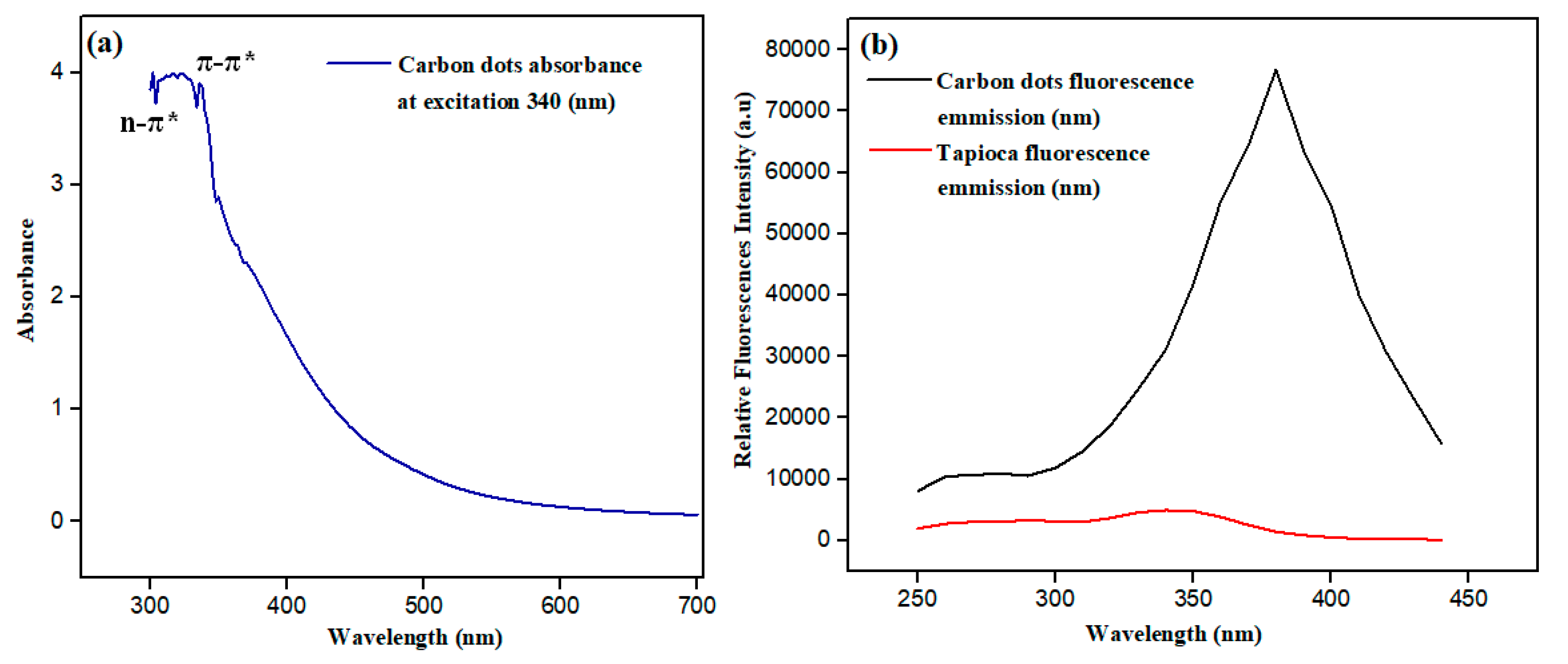
3.4. Characterization and Properties of Carbon Dots

The need to analyze carbon dots for their characteristic attributes is very essential. These can be done by determining the particle sizes and morphological patterns using high resolution devices [34]. The atomic force microscopy (AFM), high resolution transmission electron microscopy (HrTEM), and field emission scanning emission microscopic (FESEM) techniques have been utilized for this purposes.

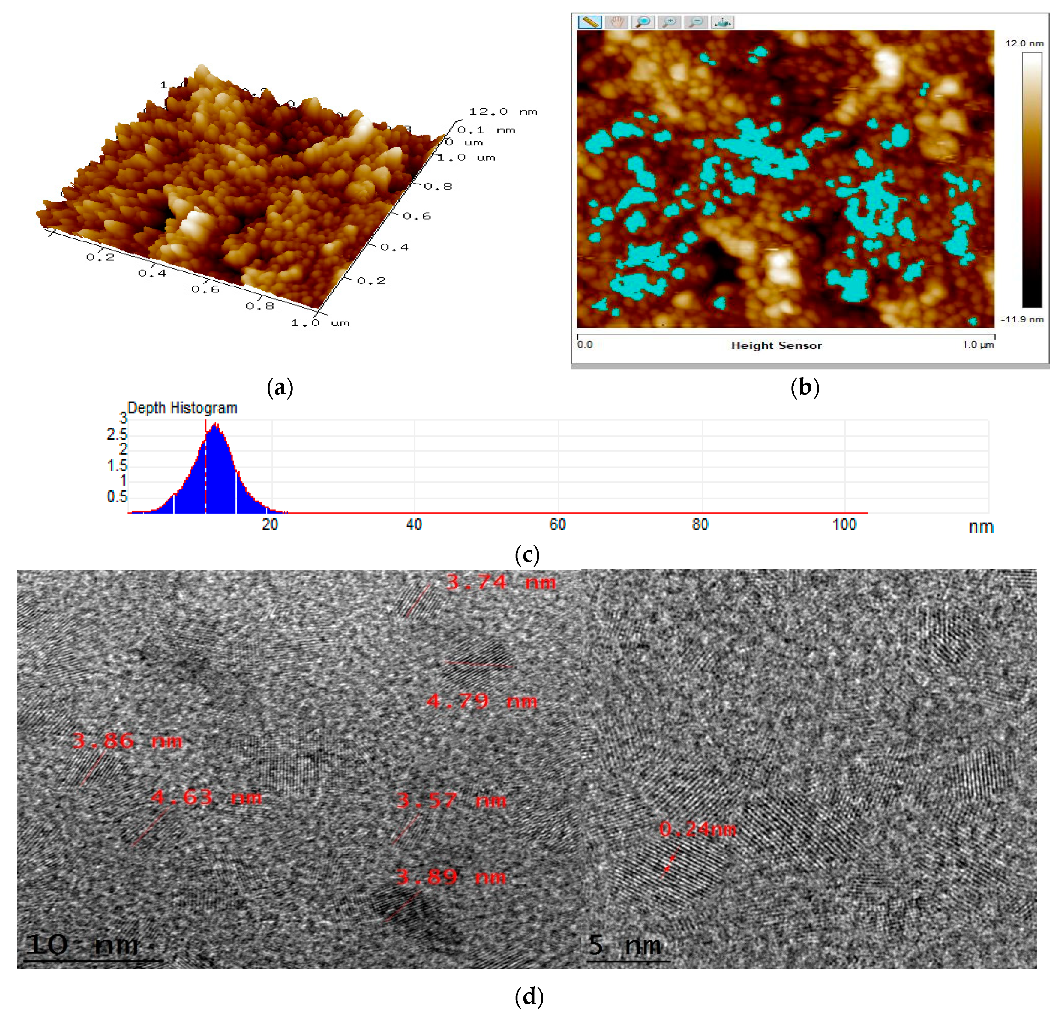
3.4.1. Atomic Force Microscopy (AFM) and High Resolution Transmission Electron Microscopy (HrTEM) of Carbon Dots (CDs)

CDs particle size distribution and morphology have been investigated (Figure 7). Figure 7a shows the three dimensional (3D) plot of the morphological pattern of carbon dots while Figure 7b depicts 62 counts of CDs with a mean height and diameter of 4.054 nm and 44.032 nm, respectively, which is a confirmation of the nano-dimension of CDs. Figure 7c represents the histogram of the 62 carbon dots count and Figure 7d is the HrTEM of carbon dots at less than 10 nm and a lattice spacing at 0.24 nm. HrTEM analysis for the carbon dots were investigated to determine the actual size and shape of the carbon dots. The image clearly depicts the synthesized CDs as well dispersed in water with a spherical petal shape and fine size distribution of about 3.0–5.0 nm in diameter shown in Figure 7.

The HrTEM provides a validation of the nano dimensions present in the synthesized CDs via hydrothermal route which is in agreement with semiconductors synthesized at the nano scale [35,36].

The CDs lattice spacing of 0.24 nm renders it suitable in membrane filtration application. More so, the sizes of CDs are below 5 nm, which means there are numerous surface sites for adsorption application purposes in wastewater treatment.

In addition,

Table 9. Analysis of the atomic force microscopy of CDs.

Parameter	Mean	Minimum	Maximum
Total Count	62	62	62
Height	4.054 (nm)	2.174 (nm)	8.486 (nm)
Area	2086.516 (nm2)	381.470 (nm2)	18,005.371 (nm2)
Diameter	44.032 (nm)	22.039 (nm)	151.411 (nm)

shows a detailed presentation of the size distribution of CDs obtained by measuring the heights, areas, and diameters of 62-single carbon dots observed under atomic force microscopy.

As presented on Table 9. The CDs mean diameter of 44.034 nm and mean area of 2086.516 nm² possess the attributes of a suitable adsorbent for adsorbing environmental pollutants [13].

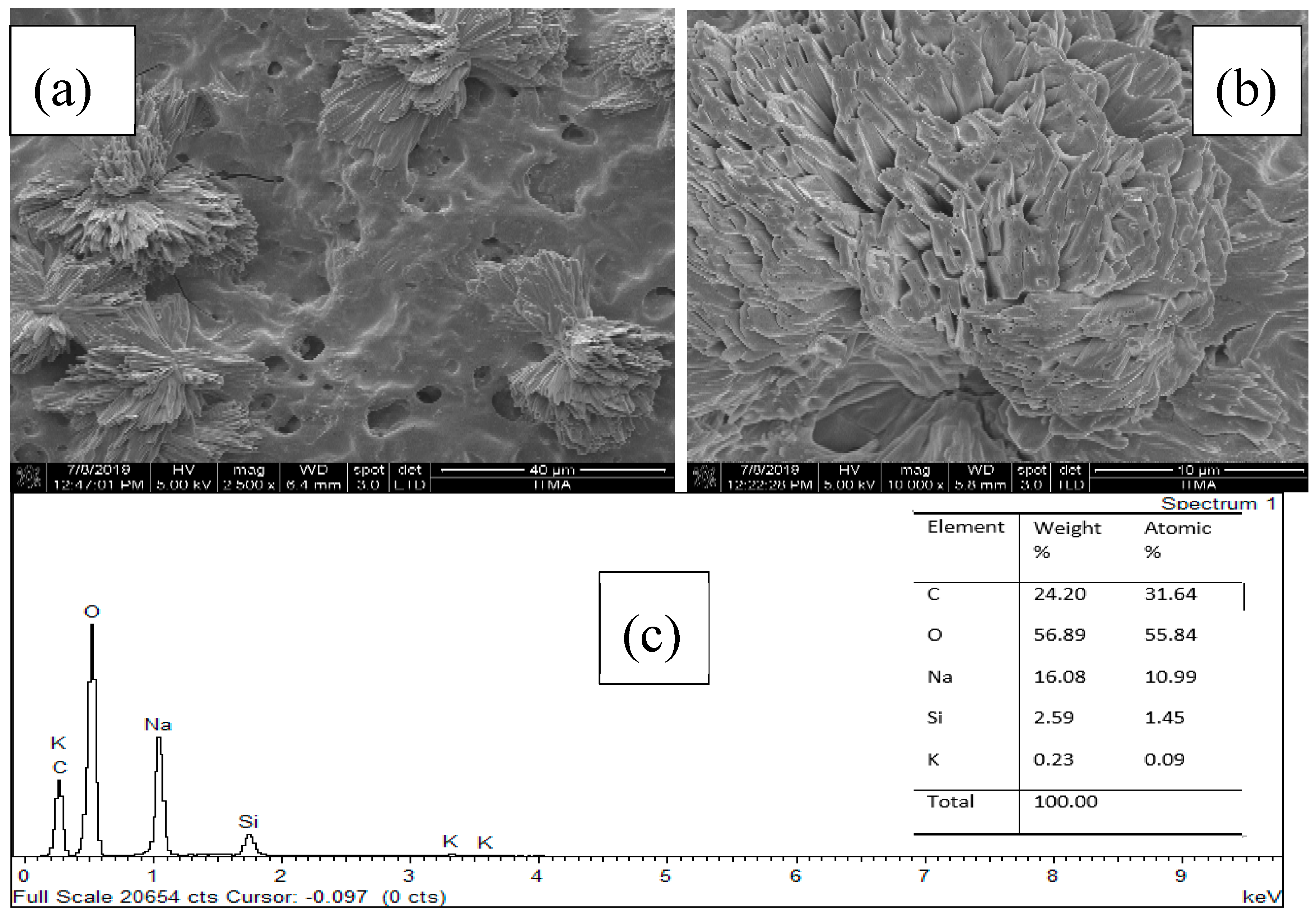
3.4.2. Field Emission Scanning Electron Microscopy (FESEM) and EDx of Tapioca-Derived Carbon Dots

From the conducted FESEM analysis, it is found that the actual shape of the CDs is in the form of a flower shaped petals, spherical in nature, as can be seen in Figure 8a,b. The EDX study determined the elemental compositions of carbon dots, and the results shows presence of C (31.64%), 0 (55.84%), Na (10.99%), Si (1.45%), and K (0.079%) as in Figure 8c. The Na signal in EDX spectrum is due to the sodium hydroxide constituent of carbon dots synthesis and silicon is as result of glass substrate for drying carbon dots during the sample preparation for FESEM.

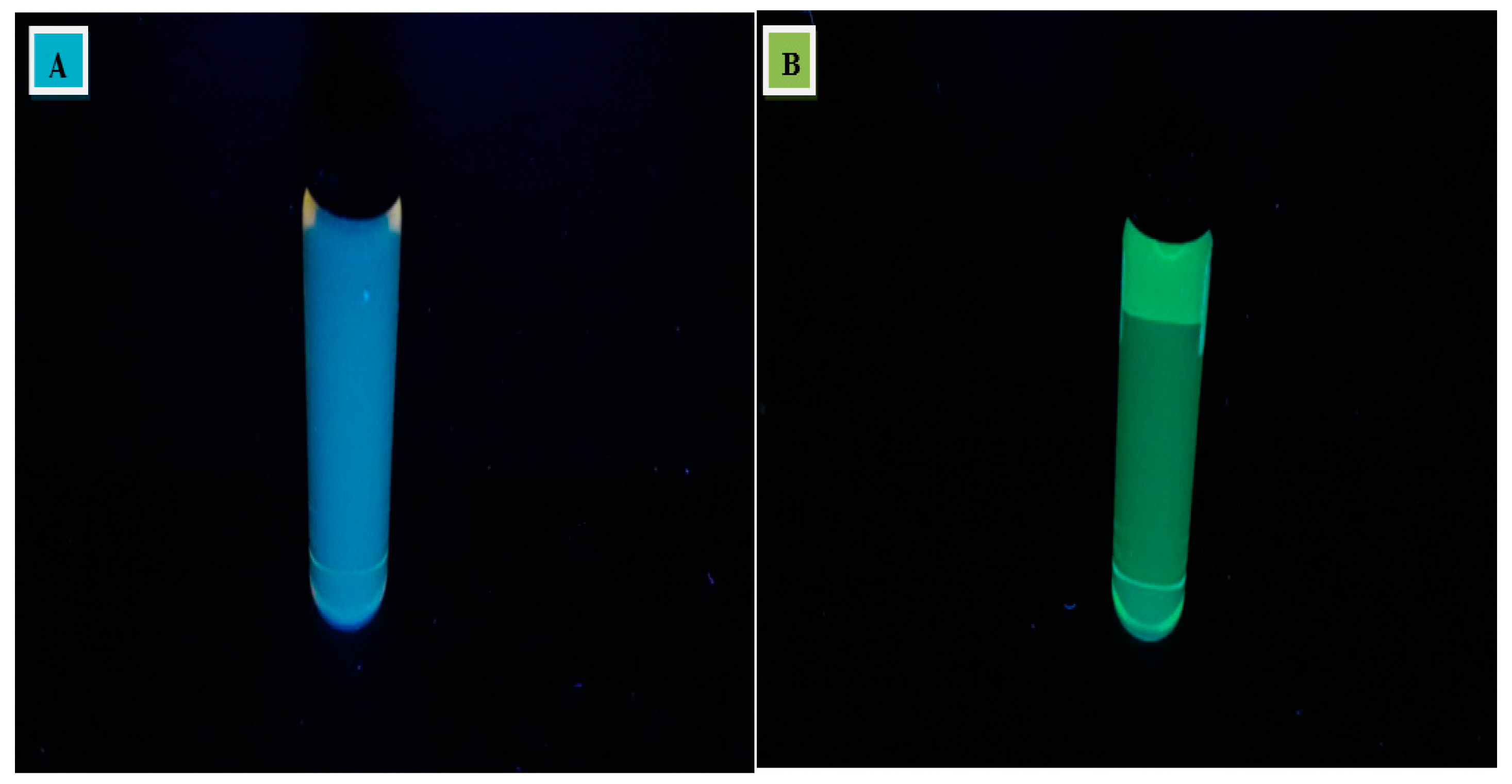
3.4.3. Properties of Carbon Dots (CDs)

The use of UV lamp to assess the quality of fluorescent carbon dots have been applied as a source to obtain a blue/green color in the near visible region of color band group. The UV irradiations absorbed by the carbon dots and excited through absorbing the energy leading to an electron excited state. The molecules of carbon dots with extended Pi-electron provides the basics for the fluorescence emission of carbon dots. The tapioca-derived carbon dot is a wavelength dependent photoluminescent ionic solution in the visible range with a surface abundant with hydroxyl and carboxylic/carboxyl moieties [13].

CDs indicated a strong optical absorption in the UV region (230–340 nm) with a tail extending to the visible range as presented in Figure 9.

Absorption shoulders in the spectrum may be due to the π-π* (pi to pi star transition) of C=C bonds or n-π* (n to pi star transition) of C=O [37]. The uniqueness of CDs is the photoluminescence emitted by it. Based on past study, it shows the dependency of intensity and wavelength emission towards excitation wavelength [38]. This is due to the different size of particles and surface chemistry and different emissive traps on CDs surface that can be related by the synthesis method.

The wavelength dependence behavior makes CDs possible to be applied in multi-color imaging applications. It has been suggested that there are separate emissions by CDs core and surface states whereby size, surface, and defects are responsible for the emission properties [13]. The color of CDs most of the time is related to the surface groups which compares to particles size and normally CDs show strong photoluminescence from blue to green wavelength. In terms of chemical properties, different synthesis methods of CDs lead to different chemical structure, such as polymer chains, oxygen based and amino-based groups [39].

The main challenge with carbon dots is the agglomeration of the particles due to strong particle interactions. It can be postulated that the agglomeration of particles over time is the very reason that these CDs emit green fluorescence since it had been left for 3 months. The resultant change in colour due to agglomeration of carbon dot particle can be observed in Figure 10 (A and B) [40].

It is well-known that there is a relationship between emission wavelength of quantum dots and particle size, i.e., the smaller the particle size is, the shorter the emission wavelength [41]. It is reasonable to speculate that this law is also applicable to carbon dots. Strong green photoluminescence offers unique superiority, because most of the current carbon dots emit blue fluorescence under UV irradiation. This kind of carbon dots had been synthesized [42].

4. Conclusions

The concept of synthesizing CDs (at zero dimension) on an industrial scale requires automation by first being able to predict the possible outcomes based upon the intended experimental factors. Thus, this study has applied tapioca as the material for optimization to achieve the set objective of large scale synthesis by means of prediction through a reliable approach of utilizing design of experiment (DoE) for a response surface methodology (RSM), to optimize a facile and effective synthesis process of fluorescent carbon dots from tapioca powder (starch) via hydrothermal synthesis route. The prediction for optimized fluorescent carbon dots synthesis from RSM is in excellent agreement with artificial neural network prediction by the Levenberg–Marquardt back propagation (LMBP) algorithm in terms of R², root mean square error and mean absolute error. Positive hidden layer sizes have resulted in the ANN prediction of PLQY of fluorescent carbon dots at 26.25% and RSM predicted value of 27.38% at R² values of 0.94 and 0.95, respectively. The best parameters values for the synthesis of carbon dots were at 170 °C for 1 h 40 min with solvent ratio of 12 mL and dosage 0.1 g. These optimization and prediction process have produced sustainable, efficient, and reliable fluorescent carbon dots, which is energy saving in a manageable time, along with a decreased dosage with optimum quality output.

Moreso, to confirm the validity of carbon dots, characterization of surface morphology and particles size carbon dots were conducted with favorable confirmations of the unique characteristics and attributes of synthesized carbon dots by hydrothermal route.

References

1. Zhou, J.; Sheng, Z.; Han, H.; Zou, M.; Li, C. Facile synthesis of fluorescent carbon dots using watermelon peel as a carbon source. Mater. Lett. 2012, 66, 222–224. [Google Scholar] [CrossRef]
2. Das, R.; Bandyopadhyay, R.; Pramanik, P. Carbon quantum dots from natural resource: A review. Mater. Today Chem. 2018, 8, 96–109. [Google Scholar] [CrossRef]
3. Witek-Krowiak, A.; Chojnacka, K.; Podstawczyk, D.; Dawiec, A.; Pokomeda, K. Application of response surface methodology and artificial neural network methods in modelling and optimization of biosorption process. Bioresour. Technol. 2014, 160, 150–160. [Google Scholar] [CrossRef] [PubMed]
4. Nwobi-Okoye, C.C.; Ochieze, B.Q. Age hardening process modeling and optimization of aluminum alloy A356/Cow horn particulate composite for brake drum application using RSM, ANN and simulated annealing. Def. Technol. 2018, 14, 336–345. [Google Scholar] [CrossRef]
5. Huang, D.; Zhao, W.; Tang, Y.; Huang, S.; Cao, W. Matching algorithm of missile tail flame based on back-propagation neural network. In Proceedings of the Fourth Seminar on Novel Optoelectronic Detection Technology and Application, Nanjing, China, 24–26 October 2017; p. 1069702. [Google Scholar]
6. Lee, J.H.; Delbruck, T.; Pfeiffer, M. Training Deep Spiking Neural Networks Using Backpropagation. Front. Mol. Neurosci. 2016, 10, 508. [Google Scholar] [CrossRef] [PubMed] [Green Version]
7. Whittington, J.C.R.; Bogacz, R. An Approximation of the Error Backpropagation Algorithm in a Predictive Coding Network with Local Hebbian Synaptic Plasticity. Neural Comput. 2017, 29, 1229–1262. [Google Scholar] [CrossRef] [PubMed] [Green Version]
8. Wisesty, U.N.; Warastri, R.S.; Puspitasari, S.Y. Leukemia and colon tumor detection based on microarray data classification using momentum backpropagation and genetic algorithm as a feature selection method. J. Phys. Conf. Ser. 2018, 971, 012018. [Google Scholar] [CrossRef]
9. Chamoli, S. ANN and RSM approach for modeling and optimization of designing parameters for a V down perforated baffle roughened rectangular channel. Alex. Eng. J. 2015, 54, 429–446. [Google Scholar] [CrossRef] [Green Version]
10. Baş, D.; Boyacı, I.H.; Boyaci, I.H. Modeling and optimization II: Comparison of estimation capabilities of response surface methodology with artificial neural networks in a biochemical reaction. J. Food Eng. 2007, 78, 846–854. [Google Scholar] [CrossRef]
11. Nazari, A.; Riahi, S. Prediction split tensile strength and water permeability of high strength concrete containing TiO2 nanoparticles by artificial neural network and genetic programming. Compos. Part B Eng. 2011, 42, 473–488. [Google Scholar] [CrossRef]
12. Nazari, A.; Riahi, S. Artificial neural networks to prediction total specific pore volume of geopolymers produced from waste ashes. Neural Comput. Appl. 2013, 22, 719–729. [Google Scholar] [CrossRef]
13. Arumugam, N.; Kim, J. Synthesis of carbon quantum dots from Broccoli and their ability to detect silver ions. Mater. Lett. 2018, 219, 37–40. [Google Scholar] [CrossRef]
14. Diao, H.; Li, T.; Zhang, R.; Kang, Y.; Liu, W.; Cui, Y.; Wei, S.; Wang, N.; Li, L.; Wang, H.; et al. Facile and green synthesis of fluorescent carbon dots with tunable emission for sensors and cells imaging. Spectrochim. Acta Part A Mol. Biomol. Spectrosc. 2018, 200, 226–234. [Google Scholar] [CrossRef] [PubMed]
15. Shahla, A.F.; Masoud, S.N.; Davood, G. Hydrothermal green synthesis of magnetic Fe3O4-carbon dots by lemon and grape fruit extracts and as a photoluminescence sensor for detecting of E. coli bacteria. Spectrochim. Acta Part A Mol. Biomol. Spectrosc. 2018, 203, 481–493. [Google Scholar]
16. Fermoso, J.; Gil, M.V.; Arias, B.; Plaza, M.; Pevida, C.; Pis, J.; Rubiera, F. Application of response surface methodology to assess the combined effect of operating variables on high-pressure coal gasification for H2-rich gas production. Int. J. Hydrog. Energy 2010, 35, 1191–1204. [Google Scholar] [CrossRef] [Green Version]
17. Lee, H.V.; Yunus, R.; Juan, J.C.; Taufiq-Yap, Y. Process optimization design for jatropha-based biodiesel production using response surface methodology. Fuel Process. Technol. 2011, 92, 2420–2428. [Google Scholar] [CrossRef] [Green Version]
18. Kefasa, H.M.; Robiah, Y.; Umer, R.; Yun, T.Y. Modified sulfonation method for converting carbonized glucose into solid acid catalyst for the esterification of palm fatty acid distillate. Fuel 2018, 229, 68–78. [Google Scholar] [CrossRef]
19. Rashid, U.; Anwar, F.; Ashraf, M.; Saleem, M.; Yusup, S. Application of response surface methodology for optimizing transesterification of Moringa oliefera oil: Biodiesel production. Energy Convers Manag. 2011, 52, 3034–3042. [Google Scholar] [CrossRef]
20. Joglekar, A.; May, A. Product excellence through design of experiments. Cereal Foods World 1987, 32, 857–868. [Google Scholar]
21. Betiku, E.; Okunsolawo, S.S.; Ajala, S.O.; Odedele, O.S. Performance evaluation of artificial neural network coupled with generic algorithm and response surface methodology in modeling and optimization of biodiesel production process parameters from shea tree (Vitellaria paradoxa) nut butter. Renew. Energy 2015, 76, 408–417. [Google Scholar] [CrossRef]
22. Da Silva Souza, D.R.; Larissa, D.C.; Joao, P.M.; Fabiano, V.P. Luminescent carbon dots obtained from cellulose. Mater. Chem. Phys. 2018, 203, 148–155. [Google Scholar] [CrossRef]
23. Horiba Scientific. A Guide to Recording Fluorescence Quantum Yield; Middlesex HA7 IBQ; Horiba UK Limited: Northampton, UK, 2018. [Google Scholar]
24. Ashby, S.P.; Thomas, J.A.; Coxon, P.R.; Bilton, M.; Brydson, R.; Pennycook, T.J.; Chao, Y. The effect of alkyl chain length on the level of capping of silicon nanoparticles produced by a one-pot synthesis route based on the chemical reduction of micelle. J. Nanoparticle Res. 2013, 15, 1425–1428. [Google Scholar] [CrossRef]
25. Sahu, S.; Behera, B.; Maiti, K.; Mohapatra, S. Simple one-step synthesis of highly luminescent carbon dots from orange juice: Application as excellent bioimaging agents. Chem. Commun. 2012, 48, 8835–8837. [Google Scholar] [CrossRef] [PubMed]
26. Jhonsi, M.A.; Thulasi, S. A novel fluorescent carbon dots derived from tamarind. Chem. Phys. Lett. 2016, 661, 179–184. [Google Scholar] [CrossRef]
27. Yadav, A.M.; Chaurasia, R.C.; Suresh, N.; Gajbhiye, P. Application of artificial neural networks and response surface methodology approaches for the prediction of oil agglomeration process. Fuel 2018, 220, 826–836. [Google Scholar] [CrossRef]
28. Ahmad, H.; Ali, A.N.; Ahmad, J.J.; Reza, K.J.; Mansour, B.; Hasan, B.; Fardin, G.P. Application of response surface methodology and artificial neuralnetwork modeling to assess non-thermal plasma efficiency insimultaneous removal of BTEX from waste gases: Effect of operatingparameters and prediction performance. Process Saf. Environ. Prot. 2018, 119, 261–270. [Google Scholar]
29. Shailendra, S.S.; Shraddha, S.; Rathindra, M.B. Preparation of Drug Eluting Natural Composite Scaffold Using Response Surface Methodology and Artificial Neural Network Approach. Tissue Eng. Regen. Med. 2018, 15, 1–13. [Google Scholar]
30. Vatankhah, E.; Semnani, D.; Prabhakaran, M.P.; Tadayon, M.; Razavi, S.; Ramakrishna, S. Artificial neural network for modeling the elastic modulus of electrospun polycaprolactone/gelatin scaffolds. Acta Biomater. 2014, 10, 709–721. [Google Scholar] [CrossRef]
31. Mukherjee, I.; Routroy, S. Comparing the performance of neural networks developed by using Levenberg–Marquardt and Quasi-Newton with the gradient descent algorithm for modelling a multiple response grinding process. Expert Syst. Appl. 2012, 39, 2397–2407. [Google Scholar] [CrossRef]
32. Wilamowski, B.M.; Yu, H. Improved Computation for Levenberg–Marquardt Training. IEEE Trans. Neural Netw. 2010, 21, 930–937. [Google Scholar] [CrossRef] [PubMed]
33. Varol, T.; Çanakçi, A.; Ozsahin, S. Prediction of effect of reinforcement content, flake size and flake time on the density and hardness of flake AA2024-SiC nanocomposites using neural networks. J. Alloy. Compd. 2018, 739, 1005–1014. [Google Scholar] [CrossRef]
34. Saud, P.S.; Pant, B.; Alam, A.-M.; Ghouri, Z.K.; Park, M.; Kim, H.-Y. Carbon quantum dots anchored TiO2 nanofibers: Effective photocatalyst for waste water treatment. Ceram. Int. 2015, 41, 11953–11959. [Google Scholar] [CrossRef]
35. Venkatesham, T.; Tanner, A.N.; Denis, O.D.; Ümit, Ö.; Indika, U.A. Ge1−xSnx alloy quantum dots with composition- tunable energy gaps and near-infrared photoluminescence. Nanoscale 2018, 10, 20296–20306. [Google Scholar]
36. Siddique, A.B.; Pramanick, A.K.; Chatterjee, S.; Ray, M. Amorphous Carbon Dots and their Remarkable Ability to Detect 2,4,6-Trinitrophenol. Sci. Rep. 2018, 8, 9770. [Google Scholar] [CrossRef] [PubMed]
37. Li, L.; Li, L.; Chen, C.; Cui, F. Green synthesis of nitrogen-doped carbon dots from ginkgo fruits and the application in cell imaging. Inorg. Chem. Commun. 2017, 86, 227–231. [Google Scholar] [CrossRef]
38. Zhao, C.; Jiao, Y.; Hu, F.; Yang, Y. Green synthesis of carbon dots from pork and application as nanosensors for uric acid detection. Spectrochim. Acta Part A Mol. Biomol. Spectrosc. 2018, 190, 360–367. [Google Scholar] [CrossRef] [PubMed]
39. Barman, M.K.; Patra, A. Current status and prospects on chemical structure driven photoluminescence behaviour of carbon dots. J. Photochem. Photobiol. C Photochem. Rev. 2018, 37, 1–22. [Google Scholar] [CrossRef]
40. Wanekaya, A.K. Applications of nanoscale carbon-based materials in heavy metal sensing and detection. Analyst 2011, 136, 4383–4391. [Google Scholar] [CrossRef]
41. Liu, H.; Ye, T.; Mao, C. Fluorescent Carbon Nanoparticles Derived from Candle Soot. Angew. Chem. Int. Ed. 2007, 46, 6473–6475. [Google Scholar] [CrossRef]
42. Zhang, Y.; Gao, Z.; Zhang, W.; Wang, W.; Chang, J.; Kai, J. Fluorescent carbon dots as nanoprobe for determination of lidocaine hydrochloride. Sens. Actuators B Chem. 2018, 262, 928–937. [Google Scholar] [CrossRef]
Figure 1. Architecture of multilayer perceptron neural network.
Processes 07 00704 g001
Figure 2. Artificial neural network model flow chart.
Processes 07 00704 g002
Figure 3. Mechanism for synthesis of carbon dots.
Processes 07 00704 g003
Figure 4. Experimental factors for 3D surface plots of tapioca powder conversion to fluorescent carbon dots.
Processes 07 00704 g004
Figure 5. Parity plots; (A) Response Surface Methodology (RSM) predicted against experimental actual values. (B) Artificial Neural Network (ANN) predicted against experimental actual values. (C) RSM predicted values against ANN predicted values.
Processes 07 00704 g005
Figure 6. Artificial neural network model coefficient of determination and error relationship of data set of fluorescent carbon dots. (a) Trained R2 output, (b) Validated R2 output, (c) Test R2 output, and (d) Overall R2 output of data set.
Processes 07 00704 g006
Figure 7. Atomic force microscopy (AFM) and high resolution transmission electron microscopy (HrTEM) of carbon dots (CDs). (a) 3D CDs particles, (b) 2D CDs particles, (c) CDs particle distribution, and (d) CDs particle sizes and lattice space.
Processes 07 00704 g007
Figure 8. FESEM at (a) 40 µm (b) 10 µm and (c) EDx of tapioca-derived carbon dots.
Processes 07 00704 g008
Figure 9. Optical properties of CDs. (a) UV-visible absorption and emission spectra of as prepared CDs dispersed in water. (b) Fluorescence emission spectra of carbon dots and reference material (Tapioca).
Processes 07 00704 g009
Figure 10. Tapioca powder as source of fluorescent carbon dots. (A) Carbon dots after synthesis emitting blue fluorescence. (B) Carbon dots emitting green fluorescence after 3 months of synthesis.
Processes 07 00704 g010