Model-Based Cost Optimization of Double-Effect Water-Lithium Bromide Absorption Refrigeration Systems

Abstract

This work presents optimization results obtained for a double-effect H₂O-LiBr absorption refrigeration system considering the total cost as minimization criterion, for a wide range of cooling capacity values. As a model result, the sizes of the process units and the corresponding operating conditions are obtained simultaneously. In this paper, the effectiveness factor of each proposed heat exchanger is considered as a model optimization variable which allows (if beneficial, according to the objective function to be minimized) its deletion from the optimal solution, therefore, helping us to determine the optimal configuration. Several optimization cases considering different target levels of cooling capacity are solved. Among the major results, it was observed that the total cost is considerably reduced when the solution heat exchanger operating at low temperature is deleted compared to the configuration that includes it. Also, it was found that the effect of removing this heat exchanger is comparatively more significant with increasing cooling capacity levels. A reduction of 9.8% in the total cost was obtained for a cooling capacity of 16 kW (11,537.2 $·year⁻¹ vs. 12,794.5 $·year⁻¹), while a reduction of 12% was obtained for a cooling capacity of 100 kW (31,338.1 $·year⁻¹ vs. 35,613.9 $·year⁻¹). The optimization mathematical model presented in this work assists in selecting the optimal process configuration, as well as determining the optimal process unit sizes and operating conditions of refrigeration systems.

1. Introduction

Compared to vapor compression cycles, the main advantage of absorption refrigeration systems (ARSs) such as water-lithium bromide (H₂O-LiBr) ARSs is that they are activated by low-level energy sources [1] (such as geothermal or solar energies) or low-grade waste heat rejected from various processes, as opposed to through the use of electric energy. On the other hand, compared to other working pairs, such as ammonia-water (NH₃-H₂O), a LiBr solution has no ozone-depleting potential or global warming effect reported in literature, in line with the Montreal, Kyoto, and Paris Accords.

The energy efficiency of a single-effect ARS is relatively low. To cope with this weakness, several papers have been published that aimed at improving the performance of single-effect H₂O-LiBr ARSs based on energy [2,3,4], exergy [4,5,6], exergo-economic [7,8], or cost [5,9] studies. Other authors have addressed such limitations by investigating other process configurations instead, including advanced configurations of multi-effect systems [10]. Among them, the double-effect schemes have comparatively received more interest, and are, in fact, the most frequently applied in industry [11,12]. Many studies on the double-effect H₂O-LiBr ARS were conducted by performing energy analyses [13,14,15], exergy analyses [15,16], and exergo-economic analyses [1,17,18]. A special feature of the double-effect ARS is its capability of running in series, parallel, and reverse parallel flow schemes according to the working solution flow through the heat exchangers and generators [11,12,13,19].

Despite the fact that systematic computer-aided methods and mathematical programming techniques have been successfully employed to optimize energy processes [20,21,22,23,24,25], not that many publications can be found for ARS [5,9,26,27,28,29,30]. These methods and techniques make it possible to optimize large mathematical models considering at the same time all the continuous and discrete decisions, which is one of the major advantages over parametric optimization approaches.

Chahartaghi et al. [27] recently studied two novel arrangements of double-effect absorption chillers with series and parallel flow, which differ from earlier conventional absorption chillers by the fact that they have an additional solution heat exchanger. They investigated the effects on the coefficient of performance (COP) of the temperature and mass flow rate of the vapor entering the high-temperature generator (HTG) and water entering the absorber (ABS). One of the results indicated that for an inlet vapor temperature to the HTG lower than 150 °C, the series cycle has a higher COP than the parallel cycle.

Lee et al. [28] employed a multi-objective genetic algorithm (MOGA) and meta-models to optimize several generators for a H₂O-LiBr absorption chiller with multiple heat sources. The integrated generation system included a HTG, a low-temperature generator (LTG), and a waste heat recovery generator (WHRG). The optimization problem consisted of the minimization of the total generation volume and the maximization of the total generation rate. It was found that the WHRG is dominant for reducing the total volume, and the HTG is dominant for improving the total generation rate.

Sabbagh and Gomez [29] proposed an optimal control strategy to operate H₂O-LiBr absorption chillers. The aim of the control strategy was to keep the cold water flow at a desired temperature (11 °C). To this end, a dynamic model consisting of differential algebraic equations (DAE) was first developed and then reformulated into a set of algebraic equations by discretizing the state and control variables using orthogonal collocation on finite elements, by dividing the time horizon into finite elements. The resulting model was implemented in the General Algebraic Modeling System (GAMS) and solved with the Interior Point OPTimization (IPOPT) solver [31]. Both step and sinusoidal perturbations of the hot water inlet temperature were studied. The results obtained are promising because, through the implementation of the optimal control strategy, the COP was significantly improved, thus reducing the operational cost and maintaining the cold water outlet temperature at the desired level.

In this paper, a mathematical model of a double-effect system with series flow configuration presented by Mussati et al. [32] is modified to consider another double-effect configuration, where the stream leaving the absorber is now split into two streams: one is passed through a solution heat exchanger (the low-temperature heat exchanger LTSHE) that is placed before the LTG, and the other is passed through another solution heat exchanger (the high-temperature heat exchanger HTSHE) that is placed before the HTG. The effectiveness factor of each solution heat exchanger is a model variable, thus making it possible to remove the corresponding solution heat exchanger, if beneficial according to the objective function that is optimized. Therefore, improved cost-effective process configurations can be found. The cost model presented by Mussati et al. [32] is employed. To the best of our knowledge, few articles deal with the simultaneous optimization approach presented in this work in order to take into account all the trade-offs existing between the model variables, which include both operation conditions and process unit sizes. The application of the proposed optimization approach leads to the improved configuration, in terms of costs, of a double-effect H₂O-LiBr absorption refrigeration system, which is the main contribution of this paper.

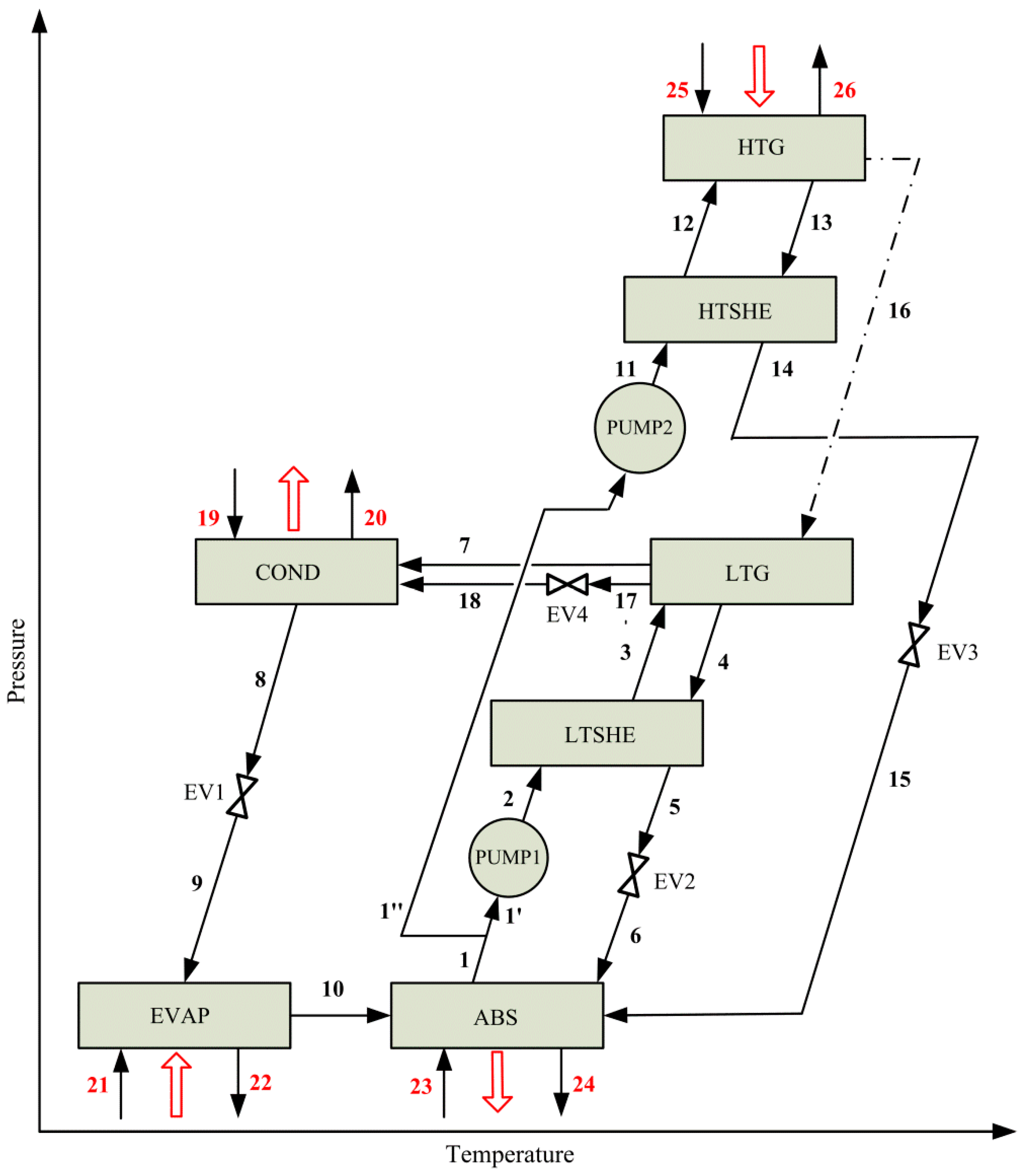
2. Process Description

As shown in Figure 1, the stream #1 that leaves the ABS is split into two streams. A fraction (stream #1’) is directed to the LTSHE through the solution pump PUMP1; it is then fed to the LTG (stream #3). The other fraction (stream #1”) is conducted to the HTSHE through the solution pump PUMP2, and then fed to the HTG (stream #12). In both generators, a vapor stream of refrigerant and a stream of concentrated LiBr solution are obtained.

The heat of the refrigerant generated in the HTG (‘energy stream’ #16)—represented by the dash-dotted line in Figure 1—is used in the LTG to produce refrigerant (stream #7) and the strong solution (stream #4). Also, low-grade waste heat rejected from other processes can be additionally used to increase the refrigerant production, which is, in fact, a remarkable feature of multi-stage configurations. This facilitates waste heat recovery as a means of implementing a circular economy strategy [33,34]. The streams #18 and #7 (refrigerant vapors) transfer their heat into the condenser COND. The condensed refrigerant (stream #8) is passed through the expansion valve EV1, and then fed to the evaporator EVAP that operates at the lowest pressure of the system. Finally, the stream #10 (vapor) is fed to the ABS and is absorbed in the resulting mixture of the strong solutions coming from LTSHE and HTSHE after passing through EV2 (stream #6) and EV3 (stream #15), respectively. The generated heat is rejected by using cooling water.

3. Mathematical Model

The mathematical model has been derived considering the following assumptions: (a) steady-state condition [12,19,35]; (b) no pressure drops and heat losses are taken into account [12,19,35]; (c) saturation condition for refrigerant streams that leave the condenser and evaporator [12,19]; (d) saturation condition for the diluted (weak) LiBr solution that leaves the absorber [12]; (e) the concentrated (strong) LiBr solutions leaving the generators are at equilibrium conditions [12]; and (f) isenthalpic process in expansion valves [19,35].

Each process unit is described by using a similar mathematical model presented by Mussati et al. [32]. The list of assumptions and the complete mathematical model (mass and energy balances) here employed are provided as Supplementary Materials related to this article. The correlations used to estimate the physicochemical properties of the LiBr solution (stream enthalpy) reported by ASHRAE [36] and the correlations used to describe the LiBr solution crystallization region given by Gilani and Ahmed [37] are also included as Supplementary Materials.

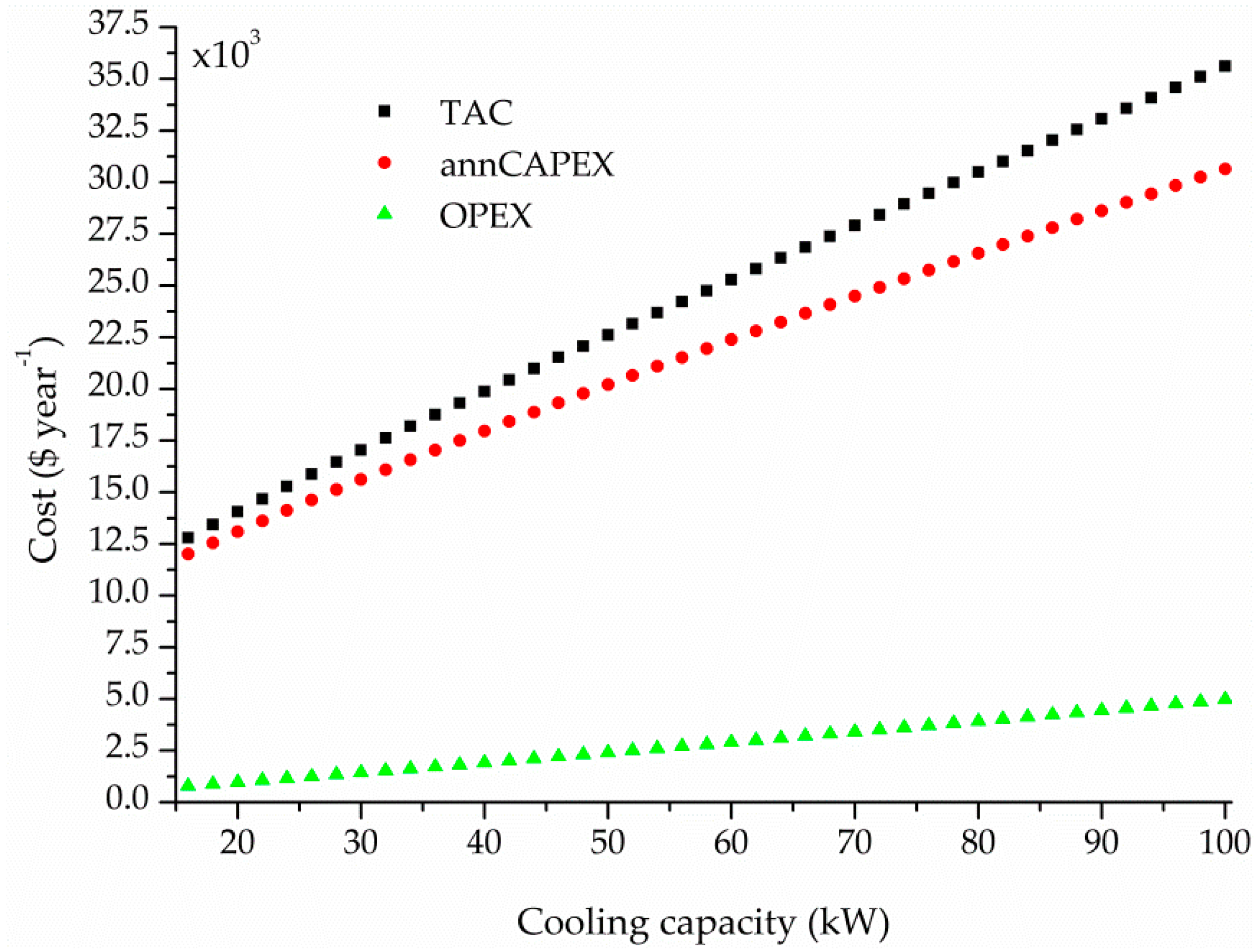
Optimization Problem: Total Annual Cost (TAC) Minimization

The optimal design consists of minimizing the TAC (Equation (1)), which accounts for the annualized capital expenditure (annCAPEX) and he operating expenditure (OPEX), while meeting the process design specifications and operation constraints for a wide range of cooling capacity levels.

$$\mathrm{TAC}=\mathrm{annCAPEX}+\mathrm{OPEX}$$

(1)

The annCAPEX is given by Equation (2). The capital recovery factor (CRF) is given by Equation (3), which is computed for a lifetime (n) of 25 years and an interest rate (i) of 10.33% [5]. The investment (Z_k) of a process unit k is given by Equation (4).

$$\mathrm{annCAPEX}=\mathrm{CRF}·{\displaystyle \sum _{\mathrm{k}}{\mathrm{Z}}_{\mathrm{k}}}$$

(2)

$$\mathrm{CRF}=\frac{\mathrm{i}·{(1+\mathrm{i})}^{\mathrm{n}}}{{(1+\mathrm{i})}^{\mathrm{n}}-1}$$

(3)

$${\mathrm{Z}}_{\mathrm{k}}={\mathrm{A}}_{\mathrm{k}}·{\left(\mathrm{f}·{\mathrm{HTA}}_{\mathrm{k}}\right)}^{{\mathrm{B}}_{\mathrm{k}}}+{\mathrm{C}}_{\mathrm{k}}$$

(4)

The OPEX is estimated by Equation (5), which includes costs associated with the heating (HU) and cooling (CU) utilities, consisting of steam (in t·year⁻¹) and cooling water (in t·year⁻¹), respectively. The unitary cost of vapor (C_HU) is 2.0 $·t⁻¹ and for cooling water (C_CU) it is 0.0195 $·t⁻¹ [5].

$$\mathrm{OPEX}={\mathrm{C}}_{\mathrm{HU}}·\mathrm{HU}+{\mathrm{C}}_{\mathrm{CU}}·\mathrm{CU}$$

(5)

The cooling capacity in EVAP (Q_EVAP) is the target design specification; it is a model parameter i.e., a known and fixed value in each optimization run. In this optimization study, Q_EVAP is parametrically varied from 16 kW to 100 kW. The optimization result provides the optimal distribution of annCAPEX and OPEX, the optimal sizes of the process units, and optimal operating conditions (stream pressure, temperature, concentration, and flow rate).

The computational tools to implement and solve the model equations were GAMS® v. 23.6.5 [38] and CONOPT 3 v. 3.14W [39], respectively. Since several nonlinear and non-convex constraints are present in the model and a local solver is used, it cannot be guaranteed that the obtained solutions correspond to the global optimum. However, based on the insights gathered from literature sources [2,5,32], the model was solved using different initial values obtaining the same solutions in all the cases. The latter forms a strong indication that the obtained solution is likely to correspond to the global optimum.

4. Results and Discussion

The optimization results obtained for a wide range of cooling capacity values and two (original and improved) process configurations are discussed. The main model parameter values are related with the cooling capacity, which is varied from 16 kW to 100 kW, and the global heat transfer coefficients, which are: 1.50 kW·m⁻²·°C⁻¹ for the evaporator, 1.0 kW·m⁻²·°C⁻¹ for the absorber, 2.50 kW·m⁻²·°C⁻¹ for the condenser, 1.50 kW·m⁻²·°C⁻¹ for the generators, and 1.0 kW·m⁻²·°C⁻¹ for the solution heat exchangers.

The external design conditions are:

–

High temperature generator (HTG): saturated steam at 160 °C.

–

Absorber (ABS) and condenser (COND): cooling water at 20 °C.

–

Evaporator (EVAP): Inlet and outlet chilled water temperatures: 13.0 °C and 10.0 °C, respectively; evaporator working temperature: 4.0 °C.

In addition, the following lower and upper bounds were imposed, respectively: 40% and 70% for LiBr concentrations, 0.1 kPa and 100 kPa for operating pressures, 0 kg·s⁻¹ and 100 kg·s⁻¹ for flow rates, and 75% and 100% for the effectiveness factors of the solution heat exchangers.

The optimization runs were performed by varying the cooling capacity from 16 kW to 100 kW. As shown in Figure 2, the minimum TAC value and the associated annCAPEX and OPEX values increase almost linearly with increasing cooling capacity levels. Also, it can be observed that the annCAPEX contribution to the TAC is significantly higher than the OPEX contribution, and that the difference between annCAPEX and OPEX increases as the cooling capacity increases. When the cooling capacity increases from 16 kW to 100 kW, the minimum TAC value and the optimal annCAPEX and OPEX values increase, respectively, 2.8, 2.5, and 6.4 times (from 12,794.5 $·year⁻¹ to 35,613.9 $·year⁻¹, from 12,013.6 $·year⁻¹ to 30,644.4 $·year⁻¹, and from 780.8 $·year⁻¹ to 4969.5 $·year⁻¹).

Figure 3 illustrates the individual contributions of the process units to annCAPEX with increasing cooling capacity levels. It can be seen that the HTG and LTG have virtually the same annCAPEX values throughout the examined range, and that they are in the same order of magnitude as the EVAP for the lowest cooling capacity levels. These values are comparatively higher than the values obtained for the other process units. For cooling capacity values between 16 and 30 kW, the contributions of the ABS and COND to the annCAPEX are similar to each other, as is the case for the HTSHE and LTSHE. Also, Figure 3 shows that the contribution of EVAP is nonlinear while the contributions of the remaining process units are practically linear. For cooling capacities higher than 18 kW, EVAP is the largest contributor to annCAPEX. When the cooling capacity increases, EVAP and ABS are the process units that increase the most rapidly in annCAPEX compared to the other process units. Indeed, ABS and EVAP increase by around 11 and 3 times, respectively, when the cooling capacity increases from 19 to 100 kW.

The optimal values of the annualized investment cost for each process unit shown in Figure 3 correspond to the optimal values of the heat transfer areas, heat loads, and driving forces shown in Figure 4a–c, respectively.

Regarding the OPEX distribution, Figure 5 shows that the contribution of the cost for steam required in the HGT as a heating source is slightly lower than the contribution of the cost for cooling water required in the COND and ABS, but the differences in cost increase with increasing cooling capacity levels. A cost difference of 75.6 $·year⁻¹ (352.6 $·year⁻¹ vs. 428.2 $·year⁻¹) is observed for a cooling capacity of 16 kW and a difference of 371.7 $·year⁻¹ (2298.9 $·year⁻¹ vs. 2670.6 $·year⁻¹) for a cooling capacity of 100 kW.

Figure 6 shows the behavior of the LiBr solution concentrations (X) of the process: weak solution (X₁) and strong solutions (X₄ and X₁₃ leaving the LTG and HTG, respectively; and X₁₅ entering the ABS), with increasing cooling capacity levels. It can be seen that that the concentration values increase with the increase of the cooling capacity, but keep similar ratios between the concentration values in the different streams.

As mentioned earlier, the effectiveness factors η_LTSHE and η_HTSHE of the solution heat exchangers LTSHE and HTSHE, respectively, are considered as (free) model variables, i.e., decision variables, as opposed to other published studies, which consider these factors as (fixed) model parameters instead, usually in the range between 65% and 90%, thus always forcing their presence in the process configuration. In this work, by allowing the heat exchanger effectiveness factor to take any value, the presence or absence of the solution heat exchangers is a result of the optimization problem. First, all the solved optimization problems considered the same lower bound for η_LTSHE and η_HTSHE of 75%. The results deserve detailed discussion because they may indicate changes in the process configuration, such as the removal of one or even both solution heat exchangers in order to obtain improved solutions, in terms of total annual costs, compared to the current optimal solutions. The optimal η_LTSHE and η_HTSHE values remain constant at the imposed lower bound (75%) throughout the range of cooling capacity values.

Then, it becomes interesting to perform new optimizations while relaxing the lower bounds imposed to η_LTSHE and η_HTSE of 75%, in order to see how these bounds affect the current optimal solutions for the same range of cooling capacity values. The obtained optimization results are presented in the forthcoming discussions.

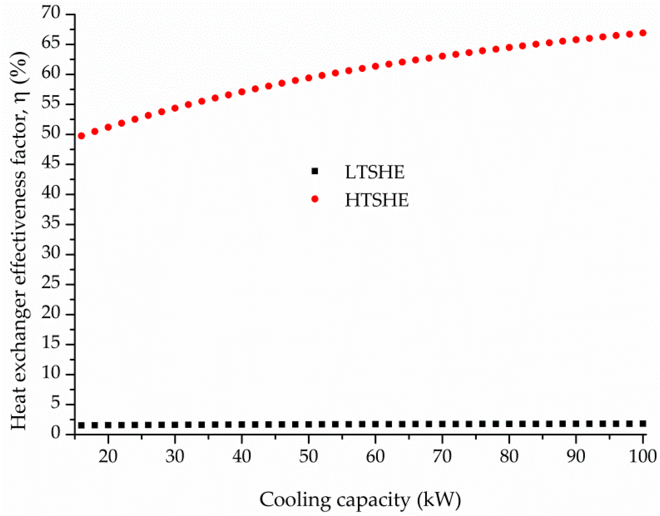
Influence of the Solution Heat Exchangers on the Optimal Solutions

The process configuration shown in Figure 1 and analyzed in the previous section—where both LTSHE and HTSHE are forced to be present—is hereafter named ‘Conf. 1’ and the one obtained in this subsection is referred as ‘Conf. 2’. In all cases, the problem that is solved is the minimization of the TAC.

Figure 7 illustrates the optimal values of both effectiveness factors η_LTSHE and η_HTSHE obtained by considering a lower bound of 1%, which, in practical terms, is virtually zero. (Note that, in this case, a ‘very small’ numerical value is imposed as the lower bound, instead of zero, to prevent numerical problems that may lead to model convergence failure). As seen in Figure 7, the obtained optimal values for η_LTSHE result in the lower bound of η_LTSHE, thus indicating that the LTSHE is removed from the configuration for all the specified cooling capacity values. However, the optimal η_HTSHE values increase logarithmically, from 49.8% to 66.9%, with increasing cooling capacity levels in the examined range. This indicates that the heat integration between the weak and strong solutions leads to cost-effective solutions only when such integration takes place in the high-temperature region of the process through HTSHE (since LTSHE in the low-temperature region is not selected in any case).

Table 1. Optimal costs obtained for configurations Conf. 1 and Conf. 2 for a cooling capacity of 16 kW.

Cost Item	Conf. 1	Conf. 2	Deviation (%)
TAC (M$·year−1)	12,794.5	11,537.2	−9.8
annCAPEX (M$·year−1)	12,013.6	10,684.3	−11.1
CAPEX (M$)	106,315.5	94,551.5	−11.1
EVAP	27,384.7	27,384.7	0
HTG	29,794.7	29,470.8	−1.1
LTG	29,447.1	29,195.3	−0.9
COND	3701.9	3802.2	+2.7
LTSHE	7135.8	121.2 (*)	−
HTSHE	5997.4	1911.9	−68.1
ABS	2853.9	2665.6	−6.6
OPEX (M$·year−1)	780.8	852.9	+9.2
Steam	352.6	405.0	+14.9
Cooling water	428.2	447.9	+4.6

(*) It is not summed in the TAC and CAPEX.

,

Table 2. Optimal values of heat transfer areas, heat loads, and driving forces obtained for configurations Conf. 1 and Conf. 2 for a cooling capacity of 16 kW.

	Heat Load (kW)		Heat Transfer Area (m2)		Driving Force (°C)
	Conf. 1	Conf. 2	Conf. 1	Conf. 2	Conf. 1	Conf. 2
EVAP	16.000	16.000	1.443	1.443	7.393	7.393
HTG	12.029	13.816	0.313	0.287	25.633	32.144
LTG	9.056	10.030	0.285	0.265	20.525	24.462
COND1	0.223	0.202	0.004	0.004	23.486	21.981
COND2	7.302	6.409	0.220	0.235	13.674	11.251
LTSHE	3.378 η = 75%	0.047 η = 1.521	0.356	0.001	9.484	44.725
HTSHE	7.375 η = 75%	3.197 η = 49.767	0.278	0.054	26.544	58.918
ABS	20.503	23.205	2.074	1.997	9.888	11.619

,

Table 3. Optimal values of operating conditions obtained for configurations Conf. 1 and Conf. 2 for a cooling capacity of 16 kW.

	Pressure (kPa)		Temperature (°C)		Solution Conc. (kg LiBr kg−1 sol.) × 100		Mass Flow Rate (kg·s−1)
Point	Conf. 1	Conf. 2	Conf. 1	Conf. 2	Conf. 1	Conf. 2	Conf. 1	Conf. 2
1	0.813	0.813	30.944	30.967	53.668	53.681	0.085	0.058
2	7.150	5.835	30.944	30.967	53.668	53.681	0.045	0.032
3	7.150	5.835	66.918	31.659	53.668	53.681	0.045	0.032
4	7.150	5.835	78.910	76.438	57.578	58.449	0.042	0.030
5	7.150	5.835	38.298	75.638	57.578	58.449	0.042	0.030
6	0.813	0.813	38.198	42.666	57.582	59.863	0.042	0.030
7	7.150	5.835	78.910	76.438	−	−	0.003	0.003
8	7.150	5.835	39.345	35.595	−	−	0.007	0.007
9	0.813	0.813	4.005	4.005	−	−	0.007	0.007
10	0.813	0.813	4.005	4.005	−	−	0.007	0.007
11	81.299	58.161	30.944	30.967	53.668	53.681	0.040	0.026
12	81.299	58.161	117.292	89.468	53.668	53.681	0.040	0.026
13	81.299	58.161	146.074	148.517	59.245	63.889	0.037	0.022
14	81.299	58.161	55.368	89.756	59.245	63.889	0.037	0.022
15	0.813	0.813	42.516	53.893	59.787	65.401	0.037	0.022
16	81.299	58.161	146.074	148.517	−	−	0.004	0.004
17	81.299	58.161	94.023	85.209	−	−	0.004	0.004
18	7.150	5.835	39.345	35.595	−	−	0.004	0.004

,

Table 4. Optimal cost values obtained for configurations Conf. 1 and Conf. 2 for a cooling capacity of 100 kW.

Cost Item	Conf. 1	Conf. 2	Deviation (%)
TAC (M$·year−1)	35,613.9	31,338.1	−12.0
annCAPEX (M$·year−1)	30,644.4	26,001.7	−15.1
CAPEX (M$)	271,189.7	230,103.8	−15.1
EVAP	75,306.6	75,306.6	0
HTG	48,532.7	45,984.3	−5.3
LTG	48,642.3	45,325.2	−6.8
COND	14,649.4	13,715.8	−6.4
LTSHE	28,054.3	514.0 (*)	−
HTSHE	23,875.4	13,062.0	−45.3
ABS	32,128.8	36,709.9	+14.3
OPEX (M$·year−1)	4969.5	5336.4	+7.4
Steam	2298.9	2358.8	+2.6
Cooling water	2670.6	2977.6	+11.5

(*) It is not summed in the TAC and CAPEX.

,

Table 5. Optimal values of heat transfer areas, heat loads, and driving forces obtained for configurations Conf. 1 and Conf. 2 for a cooling capacity of 100 kW.

	Heat Load (kW)		Heat Transfer Area (m2)		Driving Force (°C)
	Conf. 1	Conf. 2	Conf. 1	Conf. 2	Conf. 1	Conf. 2
EVAP	100.00	100.00	9.017	9.017	7.393	7.393
HTG	78.424	80.466	2.295	1.988	22.781	26.979
LTG	56.767	61.849	2.308	1.911	15.866	20.885
COND1	1.582	1.389	0.049	0.039	12.977	14.307
COND2	45.018	40.332	3.602	3.189	5.175	5.233
LTSHE	20.039 (η = 75%)	0.316 (η = 1.794%)	2.518	0.008	7.960	38.000
HTSHE	52.188 (η = 75%)	29.361 (η = 66.910%)	1.999	0.845	26.101	34.758
ABS	131.825	138.745	7.842	8.438	16.809	16.442

and

Table 6. Optimal values of operating conditions obtained for configurations Conf. 1 and Conf. 2 for a cooling capacity of 100 kW.

	Pressure (kPa)		Temperature (°C)		Solution Conc. (kg LiBr kg−1 sol.) × 100		Mass Flow Rate (kg·s−1)
Point	Conf. 1	Conf. 2	Conf. 1	Conf. 2	Conf. 1	Conf. 2	Conf. 1	Conf. 2
1	0.813	0.813	38.569	35.667	57.774	56.253	0.667	0.416
2	4.575	4.146	38.569	35.667	57.774	56.253	0.349	0.223
3	4.575	4.146	67.385	36.162	57.774	56.253	0.349	0.223
4	4.575	4.146	76.991	74.414	61.017	60.766	0.330	0.207
5	4.575	4.146	45.083	73.914	61.017	60.766	0.330	0.207
6	0.813	0.813	44.983	46.760	61.021	61.902	0.330	0.207
7	4.575	4.146	76.991	74.414	−	−	0.019	0.017
8	4.575	4.146	31.244	29.525	−	−	0.042	0.042
9	0.813	0.813	4.005	4.005	−	−	0.042	0.042
10	0.813	0.813	4.005	4.005	−	−	0.042	0.042
11	66.147	51.122	38.569	35.667	57.774	56.253	0.318	0.193
12	66.147	51.122	120.781	110.365	57.774	56.253	0.318	0.193
13	66.147	51.122	148.185	147.306	62.407	64.801	0.294	0.167
14	66.147	51.122	63.409	68.330	62.407	64.801	0.294	0.167
15	0.813	0.813	49.006	53.893	63.008	65.401	0.294	0.167
16	66.147	51.122	148.185	147.306	−	−	0.024	0.025
17	66.147	51.122	88.538	81.941	−	−	0.024	0.025
18	4.575	4.146	31.244	29.525	−	−	0.024	0.025

compare costs, process-unit sizes, and operating conditions obtained for the two configurations corresponding to the extremes of the studied cooling capacity range, i.e., for 16 kW and 100 kW.

Figure 8, Figure 9 and Figure 10 compare the optimal values of costs obtained for both configurations for the whole range of cooling capacity values. Figure 8a,b show that Conf. 2 has lower TAC and annCAPEX values, respectively, than Conf. 1 for all cooling capacity levels. However, Conf. 1 has slightly lower OPEX values than the OPEX values obtained for Conf. 2 (Figure 8c). The differences in TAC, annCAPEX, and OPEX values between Conf. 1 and Conf. 2 increase with increasing cooling capacity levels. As seen in Figure 8a,b and Table 1, at a cooling capacity of 16 kW, the TAC and annCAPEX values obtained for Conf. 2 are 9.8% and 11.1% lower than the values obtained for Conf. 1 (11,537.2 M$·year⁻¹ vs. 12,794.5 M$·year⁻¹, and 10,684.3 M$·year⁻¹ vs. 12,013.6 M$·year⁻¹, respectively). However, the OPEX in Conf. 2 is 9.2% higher than in Conf. 1 (852.9 M$·year⁻¹ vs. 780.8 M$·year⁻¹). For a cooling capacity of 100 kW, Table 4 shows that the TAC and annCAPEX values obtained for Conf. 2 are, respectively, 12% and 15.1% lower than the values obtained for Conf. 1 (31,338.1 M$·year⁻¹ vs. 35,613.9 M$·year⁻¹, and 26,001.7 M$·year⁻¹ vs. 30,644.4 M$·year⁻¹, respectively). While the OPEX for Conf. 2 is 7.4% higher than for Conf. 1 (5336.4 M$·year⁻¹ vs. 4969.5 M$·year⁻¹, respectively).

Figure 9a compares the cost for steam (heating utility) required for different cooling capacity levels between both configurations, while Figure 9b compares the cost for cooling water requirements. It can be seen that, for all cooling capacity values, the cost for steam obtained for Conf. 2 is slightly higher than the cost obtained for Conf. 1, and that the difference remains almost constant throughout the examined range (Figure 9a). The cost for cooling water is almost the same for low capacity level values; however, for higher cooling capacity levels, the cost for Conf. 2 is greater than the cost for Conf. 1, and the difference increases with increasing cooling capacity values (Figure 9b).

Figure 10 shows the investments associated with the process units obtained for Conf. 2. When comparing this figure and Figure 3 corresponding to Conf. 1, it can be seen that the trends of the individual contributions of the process units are similar for both configurations, except for LTSHE. This indicates that the elimination of LTSHE from the configuration does not modify the general trends of the investments required for the other process units as a function of the cooling capacity.

Finally, it is interesting to compare in Table 3 (16 kW) and Table 6 (100 kW) the optimal flow rate values of the weak (stream #1) and strong (stream #6) solutions for both configurations. Independently of the cooling capacity level, the optimal values of these variables obtained for Conf. 2 are significantly lower than the values obtained for Conf. 1. Moreover, all the flow rate values of the weak and strong solutions (m₁ to m₆, and m₁₁ to m₁₅) obtained for Conf. 2 are comparatively lower than the values obtained for Conf. 1 (by around 30–45% depending on the particular stream considered). For 16 kW, m₁ decreases from 0.085 kg·s⁻¹ to 0.058 kg·s⁻¹ (a 32% decrease) and m₂ from 0.045 kg·s⁻¹ to 0.032 kg·s⁻¹ (a 29% decrease). However, the weak solution concentration X₁ remains virtually unchanged for 16 kW and changes by only 2.6% for 100 kW. However, the (absolute) values are different; they are 53.7% for 16 kW and 56.2% for 100 kW, in Conf. 2.

Another interesting result, from a practical point of view, is that the optimal medium and high operating pressures obtained for Conf. 2 are also significantly lower than the values obtained for Conf. 1. Table 3 shows that the medium and high pressures for Conf. 2 are 18% and 28% lower than Conf. 1, respectively, for a cooling capacity of 16 kW. Table 6 shows that these reductions are 9% and 23%, respectively, for 100 kW. However, it should be observed that, for Conf. 2 and throughout the examined range of cooling capacity values, the LiBr concentration X₁₅ and temperature T₁₅ of stream #15 reached the values of 65.401% and 53.893 °C, respectively, which were obtained from the model constraint that describes the crystallization line. In fact, the inequality constraints that prevent crystallization became active, thus indicating that Conf. 2 operates in a region closer to the crystallization line than Conf. 1.

Finally, in order to investigate the influence of the utility costs in the optimal solutions, the same optimization problems were solved by changing the current cost parameters. Specifically, the current cooling water and steam costs were changed to 2.95 × 10⁻² $·t⁻¹ of cooling water and 84 $·t⁻¹ of steam, respectively. These numerical values are reported by Khan et al. [40] and Union Gas Limited [41], respectively. In addition, the influence of the global heat transfer coefficient values on the optimal solutions was studied. The optimization results showed that the optimal process configuration and the trends of the process variables do not vary with respect to the solutions discussed above when changes in the parameters were introduced.

5. Conclusions

This paper addressed the optimization of a double-effect H₂O-LiBr ARS through the minimization of the total annual cost for a wide range of cooling capacity values. To this end, the existing trade-offs between process configuration, sizes of the process units, and operating conditions were optimized by employing a nonlinear mathematical model, which was implemented in GAMS. Interestingly, the effectiveness factors of the solution heat exchangers, which were treated as optimization variables instead of fixed parameters, allowed us to obtain a new process configuration. The low-temperature heat exchanger is removed from the configuration throughout the examined range of cooling capacity levels, keeping only the high-temperature solution heat exchanger, indicating that the heat integration between the weak and strong LiBr solutions takes place entirely at the high-temperature zone of the process. The importance in terms of the effectiveness factor of the high-temperature solution heat exchanger increases with increasing cooling capacity levels; the sizes and operating conditions of the other process units accommodate accordingly, in order to meet the problem specifications with the minimal total annual cost. However, the improved configuration operates in a region closer to the crystallization line than the original configuration.

For a specified cooling capacity of 16 kW, the improved configuration makes it possible to reduce the total annual cost and the annualized capital expenditures by around 10% and 11%, respectively, with respect to the optimized conventional double-effect configuration, at the expense of increasing the operating expenditures by around 9%. For a cooling capacity of 100 kW, these percentages are 12%, 15%, and 7.4%, respectively. Then, the improved configuration shows better cost performances at the higher cooling capacity levels that were studied.

In future work, the proposed model will consider the variation of the heat transfer coefficients with the temperature in each process unit. Then, a superstructure-based representation embedding several candidate configurations, and thereby allowing different flow patterns, will be modeled and solved through a discrete and continuous mathematical programming model. The latter system will also include the possibility of extending the number of effects, and will make it possible to consider other heat sources.

References

1. Garousi Farshi, L.; Mahmoudi, S.M.S.; Rosen, M.A.; Yari, M.; Amidpour, M. Exergoeconomic analysis of double effect absorption refrigeration systems. Energy Convers. Manag. 2013, 65, 13–25. [Google Scholar] [CrossRef]
2. Mazzei, M.S.; Mussati, M.C.; Mussati, S.F. NLP model-based optimal design of LiBr–H2O absorption refrigeration systems. Int. J. Refrig. 2014, 38, 58–70. [Google Scholar] [CrossRef]
3. Kaynakli, O.; Kilic, M. Theoretical study on the effect of operating conditions on performance of absorption refrigeration system. Energy Convers. Manag. 2007, 48, 599–607. [Google Scholar] [CrossRef]
4. Avanessian, T.; Ameri, M. Energy, exergy, and economic analysis of single and double effect LiBr–H2O absorption chillers. Energy Build. 2014, 73, 26–36. [Google Scholar] [CrossRef]
5. Mussati, S.F.; Gernaey, K.V.; Morosuk, T.; Mussati, M.C. NLP modeling for the optimization of LiBr-H2O absorption refrigeration systems with exergy loss rate, heat transfer area, and cost as single objective functions. Energy Convers. Manag. 2016, 127, 526–544. [Google Scholar] [CrossRef]
6. Talbi, M.M.; Agnew, B. Exergy analysis: An absorption refrigerator using lithium bromide and water as the working fluids. Appl. Therm. Eng. 2000, 20, 619–630. [Google Scholar] [CrossRef]
7. Misra, R.D.; Sahoo, P.K.; Sahoo, S.; Gupta, A. Thermoeconomic optimization of a single effect water/LiBr vapour absorption refrigeration system. Int. J. Refrig. 2003, 26, 158–169. [Google Scholar] [CrossRef]
8. Kızılkan, Ö.; Şencan, A.; Kalogirou, S.A. Thermoeconomic optimization of a LiBr absorption refrigeration system. Chem. Eng. Process. Process Intensif. 2007, 46, 1376–1384. [Google Scholar] [CrossRef]
9. Rubio-Maya, C.; Pacheco-Ibarra, J.J.; Belman-Flores, J.M.; Galván-González, S.R.; Mendoza-Covarrubias, C. NLP model of a LiBr–H2O absorption refrigeration system for the minimization of the annual operating cost. Appl. Therm. Eng. 2012, 37, 10–18. [Google Scholar] [CrossRef]
10. Srikhirin, P.; Aphornratana, S.; Chungpaibulpatana, S. A review of absorption refrigeration technologies. Renew. Sustain. Energy Rev. 2001, 5, 343–372. [Google Scholar] [CrossRef]
11. Garousi, F.; Seyed, M.; Rosen, M.A.; Yari, M. A comparative study of the performance characteristics of double-effect absorption refrigeration systems. Int. J. Energy Res. 2012, 36, 182–192. [Google Scholar] [CrossRef]
12. Garousi Farshi, L.; Seyed Mahmoudi, S.M.; Rosen, M.A. Analysis of crystallization risk in double effect absorption refrigeration systems. Appl. Therm. Eng. 2011, 31, 1712–1717. [Google Scholar] [CrossRef]
13. Arun, M.B.; Maiya, M.P.; Murthy, S.S. Performance comparison of double-effect parallel-flow and series flow water–lithium bromide absorption systems. Appl. Therm. Eng. 2001, 21, 1273–1279. [Google Scholar] [CrossRef]
14. Kaushik, S.C.; Arora, A. Energy and exergy analysis of single effect and series flow double effect water–lithium bromide absorption refrigeration systems. Int. J. Refrig. 2009, 32, 1247–1258. [Google Scholar] [CrossRef]
15. Kaynakli, O.; Saka, K.; Kaynakli, F. Energy and exergy analysis of a double effect absorption refrigeration system based on different heat sources. Energy Convers. Manag. 2015, 106, 21–30. [Google Scholar] [CrossRef]
16. Talukdar, K.; Gogoi, T.K. Exergy analysis of a combined vapor power cycle and boiler flue gas driven double effect water–LiBr absorption refrigeration system. Energy Convers. Manag. 2016, 108, 468–477. [Google Scholar] [CrossRef]
17. Misra, R.D.; Sahoo, P.K.; Gupta, A. Thermoeconomic evaluation and optimization of a double-effect H2O/LiBr vapour-absorption refrigeration system. Int. J. Refrig. 2005, 28, 331–343. [Google Scholar] [CrossRef]
18. Bereche, R.P.; Palomino, R.G.; Nebra, S.A. Thermoeconomic analysis of a single and double-effect LiBr/H2O absorption refrigeration system. Int. J. Thermodyn. 2009, 12, 89–96. [Google Scholar]
19. Gebreslassie, B.H.; Medrano, M.; Boer, D. Exergy analysis of multi-effect water–LiBr absorption systems: From half to triple effect. Renew. Energy 2010, 35, 1773–1782. [Google Scholar] [CrossRef]
20. Mussati, S.F.; Aguirre, P.A.; Scenna, N.J. Novel Configuration for a Multistage Flash-Mixer Desalination System. Ind. Eng. Chem. Res. 2003, 42, 4828–4839. [Google Scholar] [CrossRef]
21. Alasino, N.; Mussati, M.C.; Scenna, N.J.; Aguirre, P. Wastewater treatment plant synthesis and design: Combined biological nitrogen and phosphorus removal. Ind. Eng. Chem. Res. 2010, 49, 8601–8612. [Google Scholar] [CrossRef]
22. Oliva, D.G.; Francesconi, J.A.; Mussati, M.C.; Aguirre, P.A. Energy efficiency analysis of an integrated glycerin processor for PEM fuel cells: Comparison with an ethanol-based system. Int. J. Hydrogen Energy 2010, 35, 709–724. [Google Scholar] [CrossRef]
23. Oliva, D.G.; Francesconi, J.A.; Mussati, M.C.; Aguirre, P.A. Modeling, synthesis and optimization of heat exchanger networks. Application to fuel processing systems for PEM fuel cells. Int. J. Hydrogen Energy 2011, 36, 9098–9114. [Google Scholar] [CrossRef]
24. Arias, A.M.; Mussati, M.C.; Mores, P.L.; Scenna, N.J.; Caballero, J.A.; Mussati, S.F. Optimization of multi-stage membrane systems for CO2 capture from flue gas. Int. J. Greenh. Gas Control 2016, 53, 371–390. [Google Scholar] [CrossRef]
25. Manassaldi, J.I.; Arias, A.M.; Scenna, N.J.; Mussati, M.C.; Mussati, S.F. A discrete and continuous mathematical model for the optimal synthesis and design of dual pressure heat recovery steam generators coupled to two steam turbines. Energy 2016, 103, 807–823. [Google Scholar] [CrossRef]
26. Gebreslassie, B.H.; Guillén-Gosálbez, G.; Jiménez, L.; Boer, D. Design of environmentally conscious absorption cooling systems via multi-objective optimization and life cycle assessment. Appl. Energy 2009, 86, 1712–1722. [Google Scholar] [CrossRef]
27. Chahartaghi, M.; Golmohammadi, H.; Shojaei, A. Performance analysis and optimization of new double effect lithium bromide–water absorption chiller with series and parallel flows. Int. J. Refrig. 2019, 97, 73–87. [Google Scholar] [CrossRef]
28. Lee, S.; Lee, J.; Lee, H.; Chung, J.; Kang, Y. Optimal design of generators for H2O/LiBr absorption chiller with multi-heat sources. Energy 2019, 167, 47–59. [Google Scholar] [CrossRef]
29. Sabbagh, A.; Gómez, J. Optimal control of single stage LiBr/water absorption chiller. Int. J. Refrig. 2018, 1–9. [Google Scholar] [CrossRef]
30. Lubis, A.; Jeong, J.; Giannetti, N.; Yamaguchi, S.; Saito, K.; Yabase, H.; Alhamid, M.I.; Nasruddin. Operation performance enhancement of single-double-effect absorption chiller. Appl. Energy 2018, 219, 299–311. [Google Scholar] [CrossRef]
31. Kawajir, Y.; Laird, C.; Wachter, A. Introduction to Ipopt: A Tutorial for Downloading, Installing, and Using Ipopt, 2087 ed. 2012. Available online: https://projects.coin-or.org/Ipopt (accessed on 23 November 2018).
32. Mussati, S.F.; Cignitti, S.; Mansouri, S.S.; Gernaey, K.V.; Morosuk, T.; Mussati, M.C. Configuration optimization of series flow double-effect water-lithium bromide absorption refrigeration systems by cost minimization. Energy Convers. Manag. 2018, 158, 359–372. [Google Scholar] [CrossRef]
33. Udugama, I.A.; Mansouri, S.S.; Mitic, A.; Flores-Alsina, X.; Gernaey, K.V. Perspectives on Resource Recovery from Bio-Based Production Processes: From Concept to Implementation. Processes 2017, 5, 48. [Google Scholar] [CrossRef]
34. Mansouri, S.S.; Udugama, I.A.; Cignitti, S.; Mitic, A.; Flores-Alsina, X.; Gernaey, K.V. Resource recovery from bio-based production processes: A future necessity? Curr. Opin. Chem. Eng. 2017, 18, 1–9. [Google Scholar] [CrossRef]
35. Dincer, I. Refrigeration Systems and Applications; Wiley: Hoboken, NJ, USA, 2003; ISBN 978-0-471-62351-9. [Google Scholar]
36. American Society of Heating, Refrigerating and Air-Conditioning Engineers. 1989 ASHRAE Handbook: Fundamentals; ASHRAE: Atlanta, GA, USA, 1989; ISBN 978-0-910110-57-0. [Google Scholar]
37. Gilani, S.I.-u.-H.; Ahmed, M.S.M.S. Solution crystallization detection for double-effect LiBr-H2O steam absorption chiller. Energy Procedia 2015, 75, 1522–1528. [Google Scholar] [CrossRef]
38. GAMS Development Corporation. General Algebraic Modeling System (GAMS) Release 23.6.5; GAMS Development Corporation: Washington, DC, USA, 2010. [Google Scholar]
39. Drud, A. CONOPT 3 Solver Manual; ARKI Consulting and Development A/S: Bagsvaerd, Denmark, 2012. [Google Scholar]
40. Khan, M.; Tahan, S.; El-Achkar, M.; Jamus, S. The study of operating an air conditioning system using Maisotsenko-Cycle. Mater. Sci. Eng. 2018, 323, 1–7. [Google Scholar] [CrossRef]
41. Union Gas Limited. Calculating the True Cost of Steam. Available online: http://members.questline.com/Article.aspx?articleID=18180&accountID=1863&nl=13848 (accessed on 23 November 2018).
Figure 1. Schematic of the studied double-effect H2O-LiBr ARS. EV1, EV2, EV3 and EV4 represent expansion valves; EVAP evaporator, ABS absorber; PUMP1 and PUMP2 solution pumps; LTSHE and HTSHE low and high temperature solution heat exchangers, respectively; LTG and HTG low- and high-temperature generators; COND condenser; dash-dotted line (stream #16) refers to an energy stream associated to the refrigerant formed in HTG.
Processes 07 00050 g001
Figure 2. Optimal values of the TAC, annCAPEX, and OPEX versus cooling capacity.
Processes 07 00050 g002
Figure 3. Optimal process-unit annCAPEX versus the cooling capacity.
Processes 07 00050 g003
Figure 4. Optimal values for each process unit of (a) heat transfer area; (b) heat loads; (c) driving force, versus the cooling capacity level.
Processes 07 00050 g004
Figure 5. Optimal distribution of the operating expenditures (OPEX) versus the cooling capacity level.
Processes 07 00050 g005
Figure 6. (a) Optimal LiBr concentration values of weak solution (X1) and strong solutions (X4 and X13 leaving the LTG and HTG, respectively; and X15 entering the ABS); (b) Optimal ABS (low), LTG (medium) and, HTG (high) operating pressure values, versus the cooling capacity level.
Processes 07 00050 g006
Figure 7. Optimal effectiveness factors η of the low-temperature solution heat exchanger (LTSHE) and the high-temperature solution heat exchanger (HTSHE) versus the cooling capacity when their lower bounds ηLB are relaxed.
Processes 07 00050 g007
Figure 8. (a) Optimal total annual cost (TAC); (b) Optimal annualized capital expenditures (annCAPEX); (c) Optimal operating expenditures (OPEX) for configurations Conf. 1 and Conf. 2 as a function of the cooling capacity level.
Processes 07 00050 g008aProcesses 07 00050 g008b
Figure 9. (a) Optimal cost values for steam requirements; (b) Optimal cost values for cooling water requirements, as a function of the cooling capacity level.
Processes 07 00050 g009
Figure 10. Optimal annualized capital expenditure (annCAPEX) values for each process unit in configuration Conf. 2 as a function of the cooling capacity level.
Processes 07 00050 g010