Toward a Distinct and Quantitative Validation Method for Predictive Process Modelling—On the Example of Solid-Liquid Extraction Processes of Complex Plant Extracts


Abstract
1. Introduction
2. Modelling of Solid-Liquid Extraction
- Shrinking Core: In the Shrinking Core model, a solvent front passes through a spherical particle. At the boundary layer between solvent and solid, the mass transfer of the target components take place. The model is based on gas-solid reactions in porous pellets [29].
- Broken and Intact Cells: The Broken and Intact Cells model is based on the idea that the target components are found both inside the plant particles, as well as in broken vacuoles or oil channels. This assumption is based on real extraction experiments in which extraction is carried out very rapidly at the beginning (near-surface components or broken vacuoles and oil channels). Subsequently, the extraction rate is greatly retarded (intact cells and oil channels). In the first case, there is no diffusion limitation, but in the second case there is a strong diffusion limitation of the extraction [30,31].
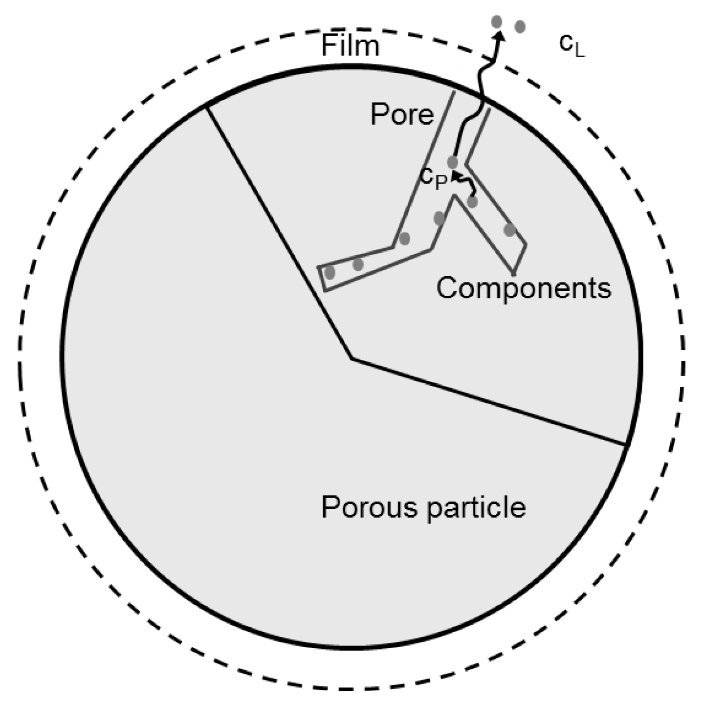
- Pore Diffusion model: The Pore Diffusion model originates from chromatography. The solvent diffuses into the porous particle and desorbs the components. Subsequently, the back diffusion and the subsequent removal take place in the core flow. Again, the basic idea of the Broken and Intact Cell model can be implemented by means of radial pore size and active substance distribution [17].
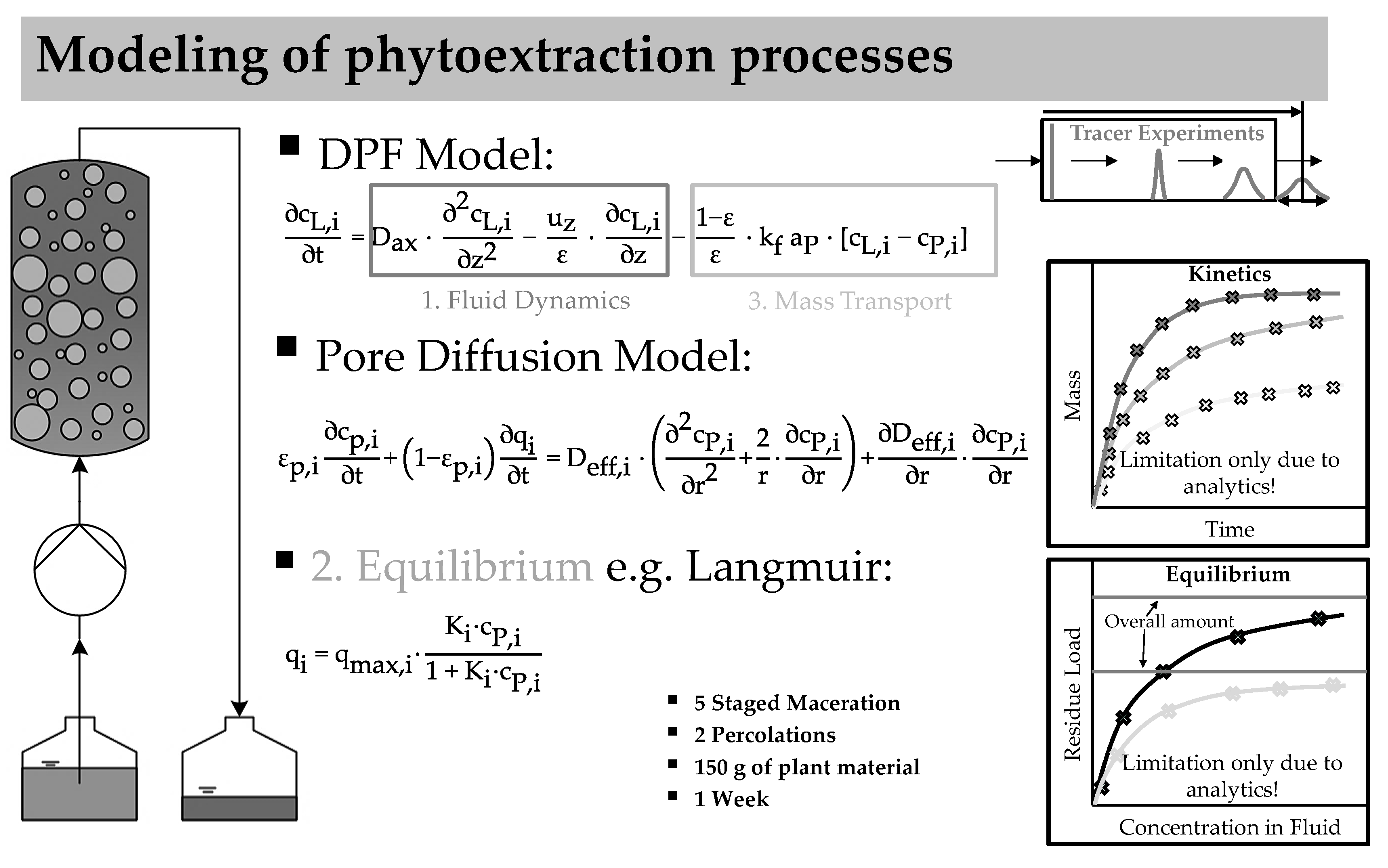
2.1. Distributed-Plug-Flow (DPF) Model
2.2. Pore Diffusion (PD) Model
2.3. Equilibrium
2.3.1. Henry
2.3.2. Freundlich
2.3.3. Langmuir
2.3.4. Modified-Langmuir
3. Model Parameter Determination
3.1. Overall Amount
- mass of plant material 20 g;
- mass of solvent 5000 g;
- density of solvent 791 g/L;
- concentration 0.03 g/L;
- and the residual moisture is 8%.
3.2. Equilibrium
- mass of plant material 20 g;
- mass of solvent 300 g;
- density of solvent 791 g/L;
- overall amount 1%;
- concentration 0.3 g/L;
- and the residual moisture is 8%.
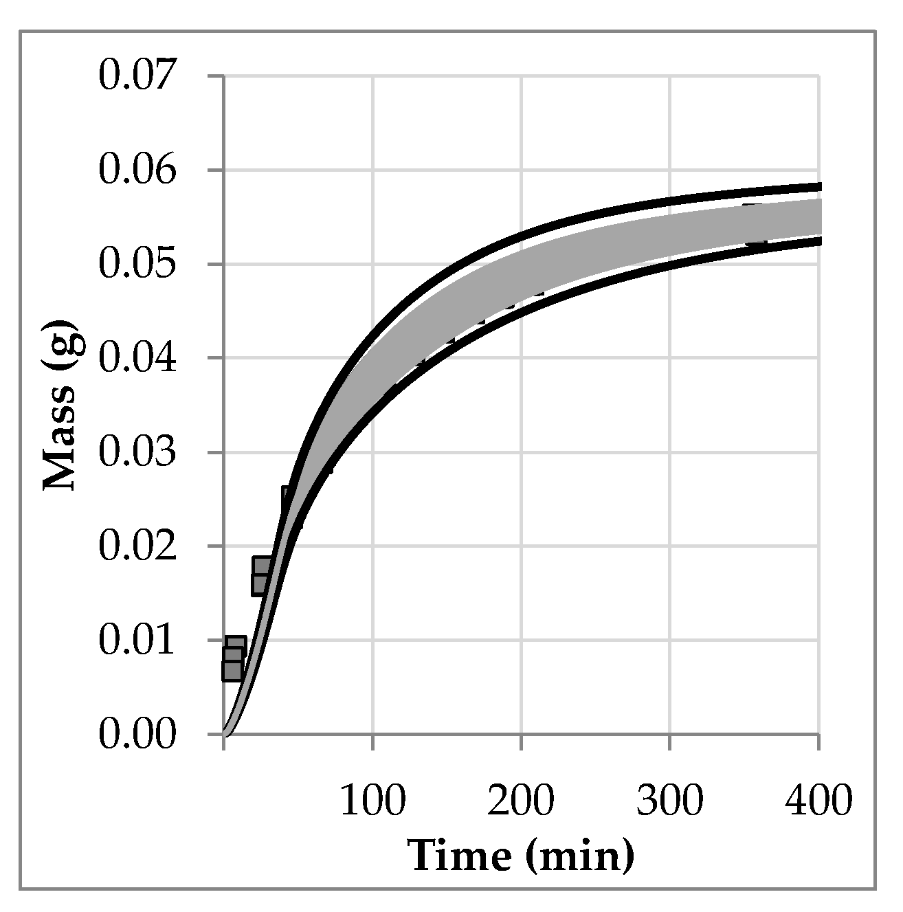
4. Model Validation
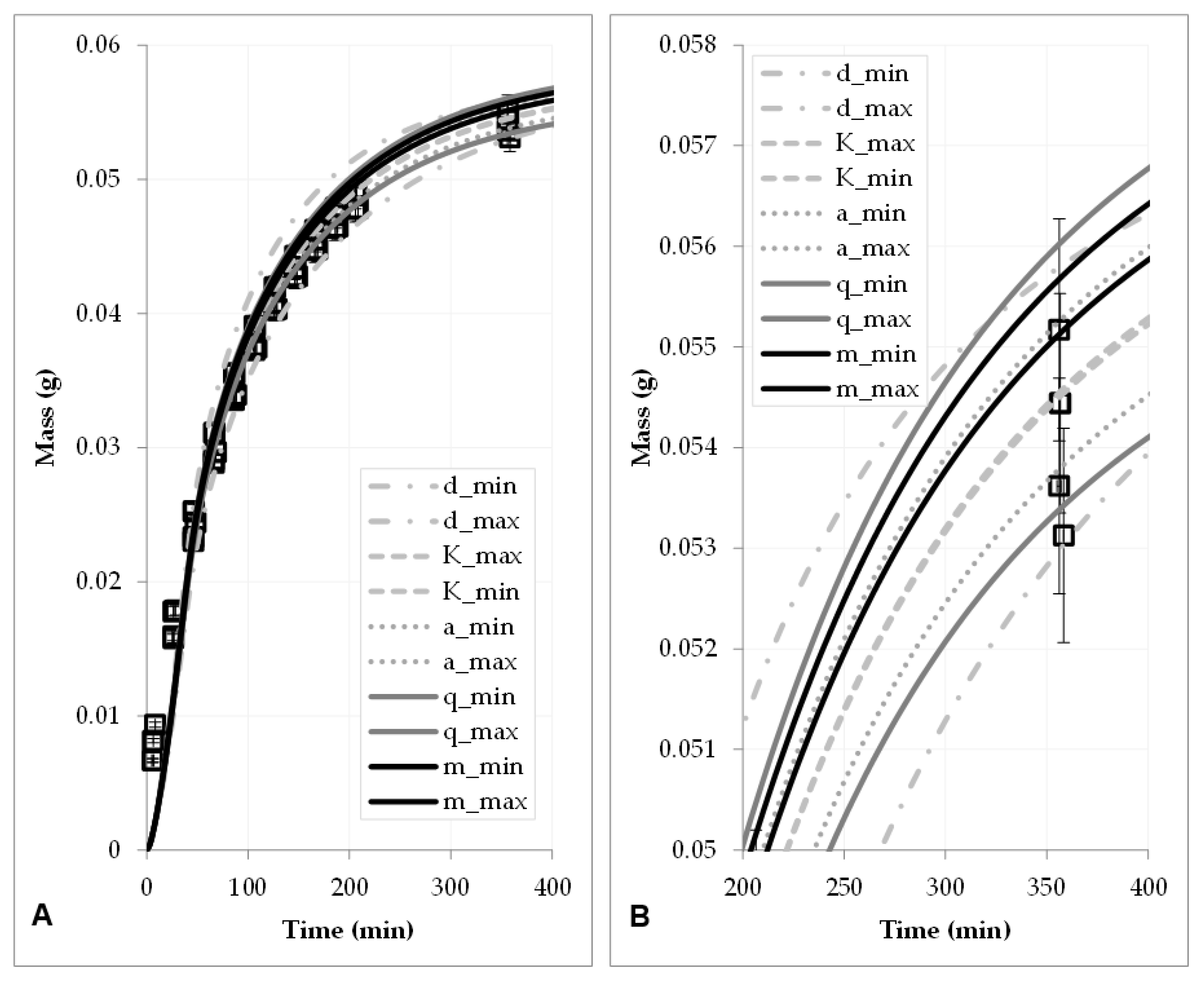
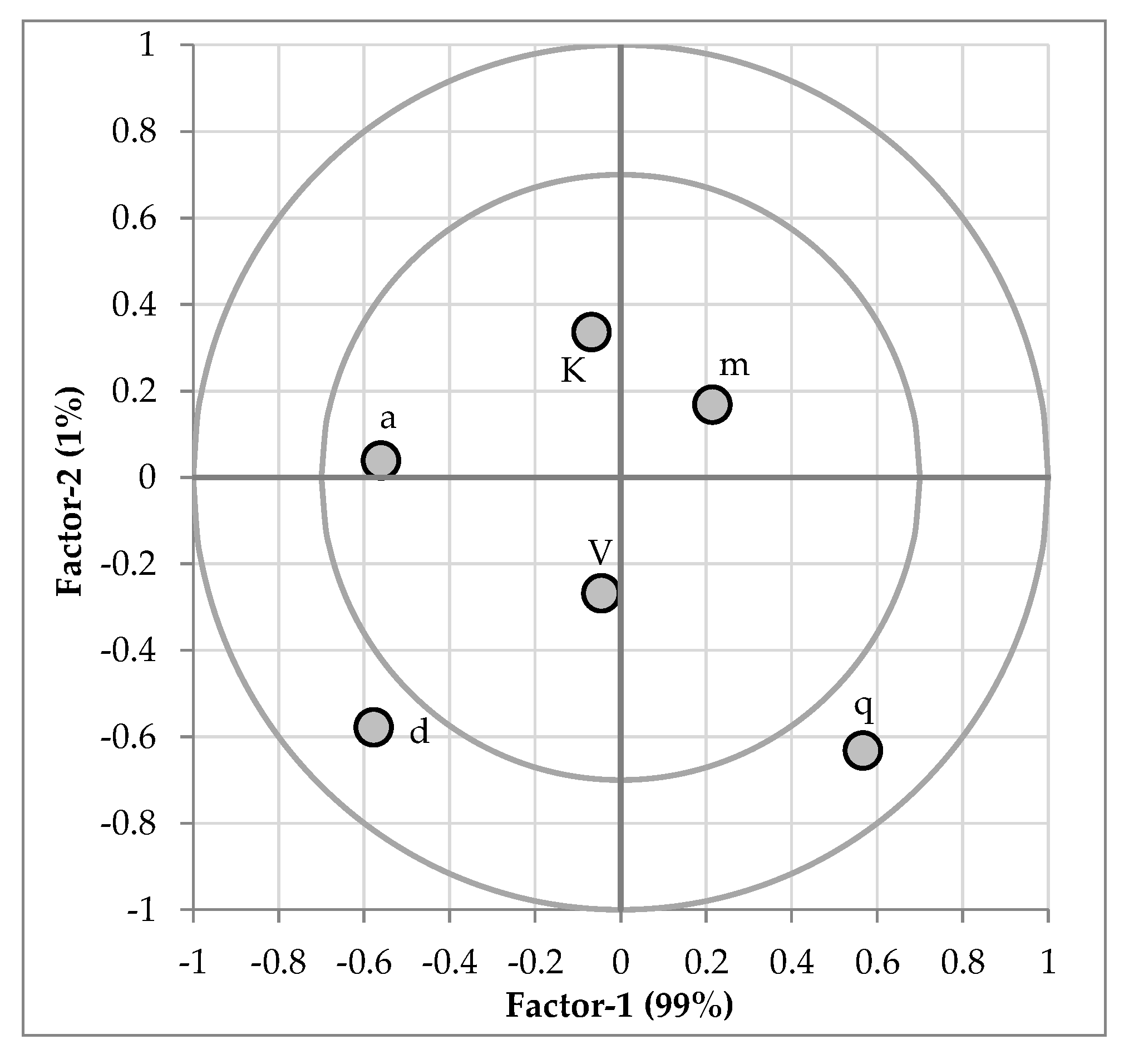
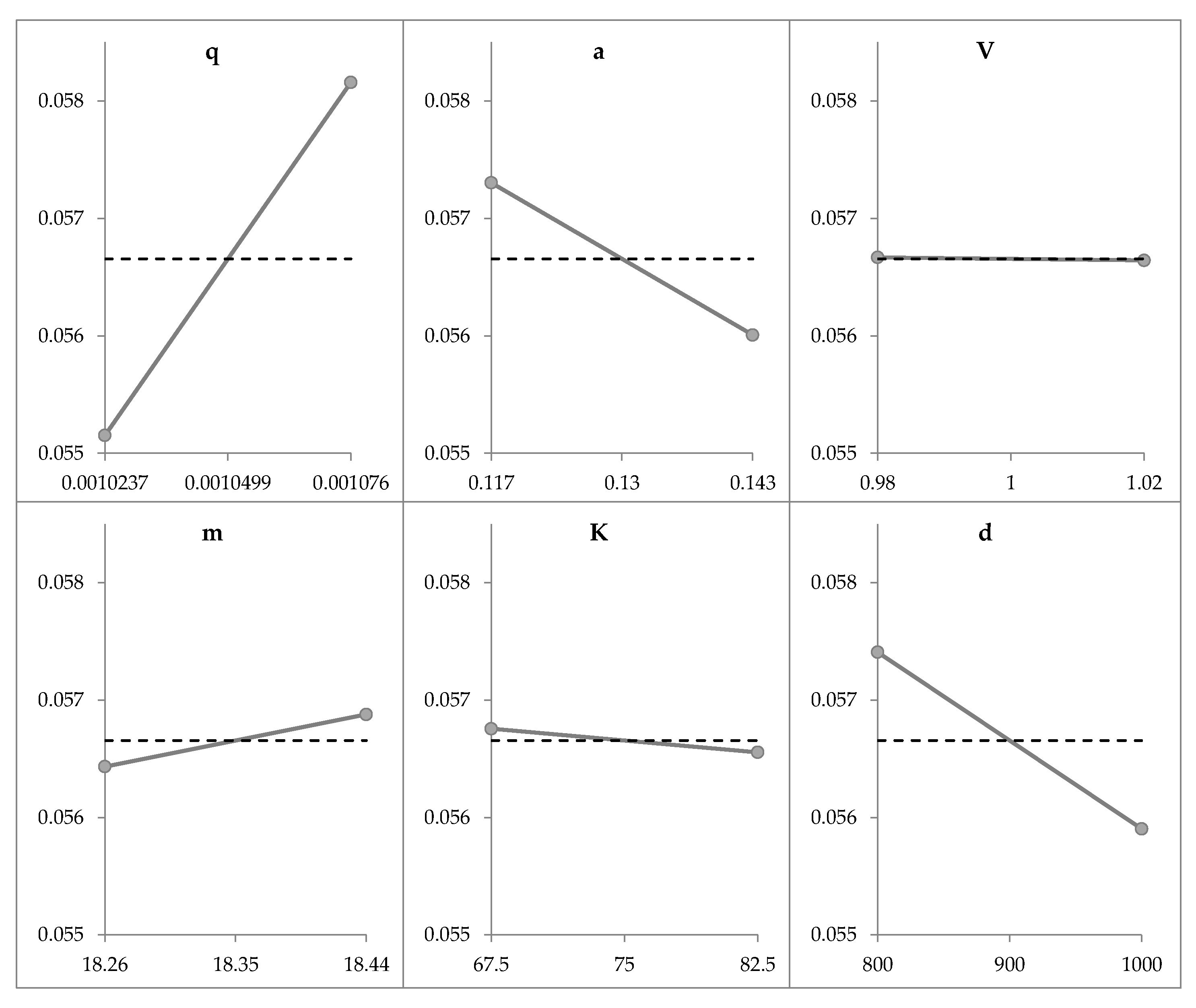
4.1. Sensitivity Analysis
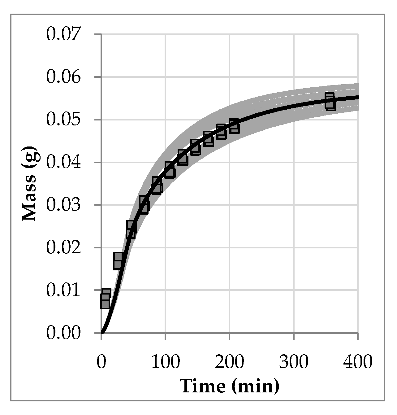
4.2. Statistical Evaluation
5. Conclusions and Discussion
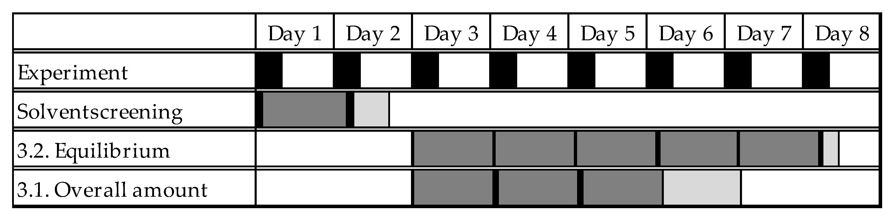
5.1. Effort Analysis
- A complete parameter determination with each experiment being run three times, takes about eight working days;
- To determine all parameters, only about 150 g of plant material and about 8 L of solvent are consumed.
5.2. Modelling in Modern Process Engineering
5.3. Workflow
Author Contributions
Acknowledgments
Conflicts of Interest
Symbols and Abbreviations
| aP | Specific surface area, 1/m |
| cL | Concentration in the liquid phase, kg/m3 |
| cP | Concentration in the porous particle, kg/m3 |
| Dax | Axial dispersion coefficient, m/s2 |
| Deff | Effective diffusion coefficient, m2/s |
| DPF | Distributed plug flow |
| KL | Equilibrium constant, m3/kg |
| kf | Mass transport coefficient, m/s |
| Pe | Péclet number |
| PEF | Pulsed electrical field |
| PF | Plug flow |
| PLS | Partial Least Square Regression |
| q | Loading, kg/m3 |
| qmax | Maximum Loading, kg/m3 |
| Re | Reynolds number |
| r | Radius, m |
| Sc | Schmidt number |
| Sh | Sherwood number |
| SME | Small and medium-sized enterprise |
| STR | Stirred tank reactor |
| t | Time, s |
| uz | Superficial velocity, m/s |
| V | Volume flow, m3/s |
| z | Coordinate in axial direction, m |
| ε | Voids fraction, - |
| ρ | Density, kg/m3 |
References
- Kennedy, R.C.; Xiang, X.; Madey, G.R.; Cosimano, T.F. Verification and Validation of Scientific and Economic Models; PROC Agent: Chicago, IL, USA, 2005. [Google Scholar]
- Oreskes, N.; Shrader-Frechette, K.; Belitz, K. Verification, validation, and confirmation of numerical models in the Earth sciences. Science 1994, 263, 641–646. [Google Scholar] [CrossRef] [PubMed]
- Ni, D.; Leonard, J.; Guin, A.; Williams, B. Systematic Approach for Validating Traffic Simulation Models. Transp. Res. Rec. 2004, 1876, 20–31. [Google Scholar] [CrossRef]
- Schleisinger, S.; Crosbie, R.E.; Gagné, R.E. Terminology for model credibility. Simulation 1979, 32, 103–104. [Google Scholar] [CrossRef]
- Jain, S. Modeling and Analysis for Semiconductor Manufacturing. In Proceedings of the 2011 Winter Simulation Conference, Phoenix, AZ, USA, 11–14 December 2011. [Google Scholar]
- Schuler, H. Prozeßsimulation; Vancouver Coastal Health: Weinheim, Germany, 1995. [Google Scholar]
- Strube, J. Prädiktive Modellierung von Trennverfahren. Chem. Ing. Tech. 2012, 84, 867. [Google Scholar] [CrossRef]
- Dechema. Roadmap Chemical Reaction Engineering: An Initiative of the ProcessNet Subject Division Chemical Reaction Engineering, 2nd ed.; Gesellschaft für Chemische Technik und Biotechnologie: Frankfurt, Germany, 2017. [Google Scholar]
- Ditz, R.; Gerard, D.; Hagels, H.; Igl, N.; Schäffler, M.; Schulz, H.; Stürtz, M.; Tegtmeier, M.; Treutwein, J.; Strube, J.; et al. Phytoextracts. Proposal towards a New Comprehensive Research Focus; Dechema: Frankfurt, Germany, 2017. [Google Scholar]
- Dechema. Empfehlungen für Grundständige Studiengänge Biotechnologie mit Naturwissenschaftlichem und Mit Verfahrenstechnischem Schwerpunkt; Dechema: Frankfurt, Germany, 2017. [Google Scholar]
- Dechema. Prozessintensivierung: Eine Standortbestimmung; Dechema: Frankfurt, Germany, 2008. [Google Scholar]
- Kreysa, G.; Marquardt, R. Biotechnologie 2020; Dechema: Frankfurt, Germany, 2005. [Google Scholar]
- Uhlenbrock, L.; Sixt, M.; Strube, J. Quality-by-Design (QbD) process evaluation for phytopharmaceuticals on the example of 10-deacetylbaccatin III from yew. Resource 2017, 3, 137–143. [Google Scholar] [CrossRef]
- Food and Drug Administration. Guidance for Industry: PAT—A Framework for Innovative Pharmaceutical Development, Manufacturing, and Quality Assurance; Food and Drug Administration: Silver Spring, MD, USA, 2004.
- Food and Drug Administration. Guidance for Industry: Q9 Quality Risk Management; Food and Drug Administration: Silver Spring, MD, USA, 2006.
- Kaßing, M. Process Development for Plant-Based Extract Production; Shaker: Aachen, Germany, 2012. [Google Scholar]
- Kaßing, M.; Jenelten, U.; Schenk, J.; Hänsch, R.; Strube, J. Combination of Rigorous and Statistical Modeling for Process Development of Plant-Based Extractions Based on Mass Balances and Biological Aspects. Chem. Eng. Technol. 2012, 35, 109–132. [Google Scholar] [CrossRef]
- Both, S.; Eggersglüß, J.; Lehnberger, A.; Schulz, T.; Schulze, T.; Strube, J. Optimizing Established Processes like Sugar Extraction from Sugar Beets—Design of Experiments versus Physicochemical Modeling. Chem. Eng. Technol. 2013, 36, 2125–2136. [Google Scholar] [CrossRef]
- Both, S. Systematische Verfahrensentwicklung für Pflanzlich Basierte Produkte im Regulatorischen Umfeld; Shaker: Aachen, Germany, 2015. [Google Scholar]
- Both, S.; Chemat, F.; Strube, J. Extraction of polyphenols from black tea—Conventional and ultrasound assisted extraction. Ultrason. Sonochem. 2014, 21, 1030–1034. [Google Scholar] [CrossRef] [PubMed]
- Both, S.; Koudous, I.; Jenelten, U.; Strube, J. Model-based equipment-design for plant-based extraction processes—Considering botanic and thermodynamic aspects. C. R. Chim. 2014, 17, 187–196. [Google Scholar] [CrossRef]
- Koudous, I. Stoffdatenbasierte Verfahrensentwicklung zur Isolierung von Wertstoffen aus Pflanzenextrakten; Shaker: Herzogenrath, Germany, 2017. [Google Scholar]
- Sixt, M.; Koudous, I.; Strube, J. Process design for integration of extraction, purification and formulation with alternative solvent concepts. C. R. Chim. 2016, 19, 733–748. [Google Scholar] [CrossRef]
- Sixt, M.; Strube, J. Systematic and Model-Assisted Evaluation of Solvent Based- or Pressurized Hot Water Extraction for the Extraction of Artemisinin from Artemisia annua L. Processes 2017, 5, 86. [Google Scholar] [CrossRef]
- Sixt, M.; Strube, J. Pressurized hot water extraction of 10-deacetylbaccatin III from yew for industrial application. Resource 2017, 3, 177–186. [Google Scholar] [CrossRef]
- Sattler, K. Thermische Trennverfahren: Grundlagen, Auslegung, Apparate; Wiley-VCH: Weinheim, Germany, 2001. [Google Scholar]
- Chémat, F.; Strube, J. Green Extraction of Natural Products. Theory and Practice; Wiley-VCH Verlag: Weinheim, Germany, 2015. [Google Scholar]
- Kaßing, M.; Jenelten, U.; Schenk, J.; Strube, J. A New Approach for Process Development of Plant-Based Extraction Processes. Chem. Eng. Technol. 2010, 33, 377–387. [Google Scholar] [CrossRef]
- Levenspiel, O. Chemical Reaction Engineering, 3rd ed.; Wiley: New York, NY, USA, 1999. [Google Scholar]
- Sovová, H. Rate of the vegetable oil extraction with supercritical CO2-I. Modelling of extraction curves. Chem. Eng. Sci. 1994, 49, 409–414. [Google Scholar] [CrossRef]
- Sovová, H. Mathematical model for supercritical fluid extraction of natural products and extraction curve evaluation. J. Supercrit. Fluids 2005, 33, 35–52. [Google Scholar] [CrossRef]
- Akgün, M.; Akgün, N.A.; Dinçer, S. Extraction and Modeling of Lavender Flower Essential Oil Using Supercritical Carbon Dioxide. Ind. Eng. Chem. Res. 2000, 39, 473–477. [Google Scholar] [CrossRef]
- Al-Jabari, M. Modeling analytical tests of supercritical fluid extraction from solids with langmuir kinetics. Chem. Eng. Commun. 2003, 190, 1620–1640. [Google Scholar] [CrossRef]
- Bulley, N.R.; Fattori, M.; Meisen, A.; Moyls, L. Supercritical fluid extraction of vegetable oil seeds. J. Am. Oil Chem. Soc. 1984, 61, 1362–1365. [Google Scholar] [CrossRef]
- Cacace, J.E.; Mazza, G. Mass transfer process during extraction of phenolic compounds from milled berries. J. Food Eng. 2003, 59, 379–389. [Google Scholar] [CrossRef]
- Carrín, M.E.; Crapiste, G.H. Mathematical modeling of vegetable oil-solvent extraction in a multistage horizontal extractor. J. Food Eng. 2008, 85, 418–425. [Google Scholar] [CrossRef]
- Catchpole, O.J.; Grey, J.B.; Smallfield, B.M. Near-critical extraction of sage, celery, and coriander seed. J. Supercrit. Fluids 1996, 9, 273–279. [Google Scholar] [CrossRef]
- Chalermchat, Y.; Fincan, M.; Dejmek, P. Pulsed electric field treatment for solid-liquid extraction of red beetroot pigment: Mathematical modelling of mass transfer. J. Food Eng. 2004, 64, 229–236. [Google Scholar] [CrossRef]
- Chia, S.L.; Sulaiman, R.; Boo, H.C.; Muhammad, K.; Umanan, F.; Chong, G.H. Modeling of Rice Bran Oil Yield and Bioactive Compounds Obtained Using Subcritical Carbon Dioxide Soxhlet Extraction (SCDS). Ind. Eng. Chem. Res. 2015, 54, 8546–8553. [Google Scholar] [CrossRef]
- Cocero, M.J.; García, J. Mathematical model of supercritical extraction applied to oil seed extraction by CO2 + saturated alcohol—I. Desorption model. J. Supercrit. Fluids 2001, 20, 229–243. [Google Scholar] [CrossRef]
- De França, L.F.; Meireles, M.A.A. Modeling the extraction of carotene and lipids from pressed palm oil (Elaes guineensis) fibers using supercritical CO2. J. Supercrit. Fluids 2000, 18, 35–47. [Google Scholar] [CrossRef]
- Del Valle, J.M.; Napolitano, P.; Fuentes, N. Estimation of Relevant Mass Transfer Parameters for the Extraction of Packed Substrate Beds Using Supercritical Fluids. Ind. Eng. Chem. Res. 2000, 39, 4720–4728. [Google Scholar] [CrossRef]
- Del Valle, J.M.; Jiménez, M.; Napolitano, P.; Zetzl, C.; Brunner, G. Supercritical carbon dioxide extraction of pelletized Jalapeño peppers. J. Sci. Food Agric. 2003, 83, 550–556. [Google Scholar] [CrossRef]
- Del Valle, J.M.; de la Fuente Juan, C.; Cardarelli, D.A. Contributions to supercritical extraction of vegetable substrates in Latin America. J. Food Eng. 2005, 67, 35–57. [Google Scholar] [CrossRef]
- Del Valle, J.M.; de la Fuente Juan, C. Supercritical CO2 extraction of oilseeds: Review of kinetic and equilibrium models. Crit. Rev. Food. Sci. Nutr. 2006, 46, 131–160. [Google Scholar] [CrossRef] [PubMed]
- Diankov, S.; Simeonov, E.; Tomova, K. Modelling of Multistage Extraction Kinetics for Nicotiana tabacum L.—Water System. J. Univ. Chem. Technol. Metall. 2008, 43, 119–124. [Google Scholar]
- Egorov, A.G.; Salamatin, A.A. Bidisperse Shrinking Core Model for Supercritical Fluid Extraction. Chem. Eng. Technol. 2015, 38, 1203–1211. [Google Scholar] [CrossRef]
- Espinoza-Pérez, J.D.; Vargas, A.; Robles-Olvera, V.J.; Rodríguez-Jimenes, G.C.; Garcia-Alvarado, M.A. Mathematical modeling of caffeine kinetic during solid-liquid extraction of coffee beans. J. Food Eng. 2007, 81, 72–78. [Google Scholar] [CrossRef]
- Esquível, M.M.; Bernardo-Gil, M.G.; King, M.B. Mathematical models for supercritical extraction of olive husk oil. J. Supercrit. Fluids 1999, 16, 43–58. [Google Scholar] [CrossRef]
- Ferreira, S.R.S.; Meireles, M.A.A. Modeling the supercritical fluid extraction of black pepper (Piper nigrum L.) essential oil. J. Food Eng. 2002, 54, 263–269. [Google Scholar] [CrossRef]
- Fiori, L.; Calcagno, D.; Costa, P. Sensitivity analysis and operative conditions of a supercritical fluid extractor. J. Supercrit. Fluids 2007, 41, 31–42. [Google Scholar] [CrossRef]
- Fiori, L.; Basso, D.; Costa, P. Seed oil supercritical extraction: Particle size distribution of the milled seeds and modeling. J. Supercrit. Fluids 2008, 47, 174–181. [Google Scholar] [CrossRef]
- Fiori, L.; Basso, D.; Costa, P. Supercritical extraction kinetics of seed oil: A new model bridging the ‘broken and intact cells’ and the ‘shrinking-core’ models. J. Supercrit. Fluids 2009, 48, 131–138. [Google Scholar] [CrossRef]
- Goodarznia, I.; Eikani, M.H. Supercritical carbon dioxide extraction of essential oils. Chem. Eng. Sci. 1998, 53, 1387–1395. [Google Scholar] [CrossRef]
- Goto, M.; Smith, J.M.; McCoy, B.J. Kinetics and mass transfer for supercritical fluid extraction of wood. Ind. Eng. Chem. Res. 1990, 29, 282–289. [Google Scholar] [CrossRef]
- Goto, M.; Sato, M.; Hirose, T. Extraction of Peppermint Oil by Supercritical Carbon Dioxide. J. Chem. Eng. Jpn. 1993, 26, 401–407. [Google Scholar] [CrossRef]
- Goto, M.; Roy, B.C.; Hirose, T. Shrinking-core leaching model for supercritical-fluid extraction. J. Supercrit. Fluids 1996, 9, 128–133. [Google Scholar] [CrossRef]
- Guerrero, M.S.; Torres, J.S.; Nunez, M.J. Extraction of polyphenols from white distilled grape pomace: Optimization and modelling. Bioresour. Technol. 2008, 99, 1311–1318. [Google Scholar] [CrossRef] [PubMed]
- Ji, J.-B.; Lu, X.-H.; Cai, M.-Q.; Xu, Z.-C. Improvement of leaching process of Geniposide with ultrasound. Ultrason. Sonochem. 2006, 13, 455–462. [Google Scholar] [CrossRef] [PubMed]
- Jokic, S.; Svilovic, S.; Vidovic, S. Modelling the supercritical CO2 extraction kinetics of soybean oil. Croat. J. Food Sci. Technol. 2015, 7, 52–57. [Google Scholar] [CrossRef]
- Kim, K.H.; Hong, J. Desorption kinetic model for supercritical fluid extraction of spearmint leaf oil. Sep. Sci. Technol. 2001, 36, 1437–1450. [Google Scholar] [CrossRef]
- Kim, K.H.; Hong, J. A mass transfer model for super- and near-critical CO2 extraction of spearmint leaf oil. Sep. Sci. Technol. 2002, 37, 2271–2288. [Google Scholar] [CrossRef]
- Lee, A.K.K.; Bulley, N.R.; Fattori, M.; Meisen, A. Modelling of supercritical carbon dioxide extraction of Canola oilseed in fixed beds. J. Am. Oil Chem. Soc. 1986, 63, 921–925. [Google Scholar] [CrossRef]
- López-Padilla, A.; Ruiz-Rodriguez, A.; Reglero, G.; Fornari, T. Supercritical carbon dioxide extraction of Calendula officinalis: Kinetic modeling and scaling up study. J. Supercrit. Fluids 2017, 130, 292–300. [Google Scholar] [CrossRef]
- Lucas, S.; Calvo, M.P.; García-Serna, J.; Palencia, C.; Cocero, M.J. Two-parameter model for mass transfer processes between solid matrixes and supercritical fluids: Analytical solution. J. Supercrit. Fluids 2007, 41, 257–266. [Google Scholar] [CrossRef]
- Machmudah, S.; Sulaswatty, A.; Sasaki, M.; Goto, M.; Hirose, T. Supercritical CO2 extraction of nutmeg oil: Experiments and modeling. J. Supercrit. Fluids 2006, 39, 30–39. [Google Scholar] [CrossRef]
- Macías-Sánchez, M.D.; Serrano, C.M.; Rodríguez, M.R.; Martínez de la Ossa, E. Kinetics of the supercritical fluid extraction of carotenoids from microalgae with CO2 and ethanol as cosolvent. Chem. Eng. J. 2009, 150, 104–113. [Google Scholar] [CrossRef]
- Madras, G.; Thibaud, C.; Erkey, C.; Akgerman, A. Modeling of supercritical extraction of organics from solid matrices. AIChE J. 1994, 40, 777–785. [Google Scholar] [CrossRef]
- Mantell, C.; Rodríguez, M.; Martínez de la Ossa, E. Semi-batch extraction of anthocyanins from red grape pomace in packed beds: Experimental results and process modelling. Chem. Eng. Sci. 2002, 57, 3831–3838. [Google Scholar] [CrossRef]
- Marrone, C.; Poletto, M.; Reverchon, E.; Stassi, A. Almond oil extraction by supercritical CO2: Experiments and modelling. Chem. Eng. Sci. 1998, 53, 3711–3718. [Google Scholar] [CrossRef]
- Martínez, J.; Monteiro, A.R.; Rosa, P.T.V.; Marques, M.O.M.; Meireles, M.A.A. Multicomponent Model To Describe Extraction of Ginger Oleoresin with Supercritical Carbon Dioxide. Ind. Eng. Chem. Res. 2003, 42, 1057–1063. [Google Scholar] [CrossRef]
- Nagy, B.; Simándi, B. Effects of particle size distribution, moisture content, and initial oil content on the supercritical fluid extraction of paprika. J. Supercrit. Fluids 2008, 46, 293–298. [Google Scholar] [CrossRef]
- Özkal, S.G.; Yener, M.E.; Bayındırlı, L. Mass transfer modeling of apricot kernel oil extraction with supercritical carbon dioxide. J. Supercrit. Fluids 2005, 35, 119–127. [Google Scholar] [CrossRef]
- Peker, H.; Srinivasan, M.P.; Smith, J.M.; McCoy, B.J. Caffeine extraction rates from coffee beans with supercritical carbon dioxide. AIChE J. 1992, 38, 761–770. [Google Scholar] [CrossRef]
- Perrut, M.; Clavier, J.Y.; Poletto, M.; Reverchon, E. Mathematical Modeling of Sunflower Seed Extraction by Supercritical CO2. Ind. Eng. Chem. Res. 1997, 36, 430–435. [Google Scholar] [CrossRef]
- Pinelo, M.; Sineiro, J.; Núñez, M.J. Mass transfer during continuous solid-liquid extraction of antioxidants from grape byproducts. J. Food Eng. 2006, 77, 57–63. [Google Scholar] [CrossRef]
- Poletto, M.; Reverchon, E. Comparison of Models for Supercritical Fluid Extraction of Seed and Essential Oils in Relation to the Mass-Transfer Rate. Ind. Eng. Chem. Res. 1996, 35, 3680–3686. [Google Scholar] [CrossRef]
- Reis-Vasco, E.M.C.; Coelho, J.A.P.; Palavra, A.M.F.; Marrone, C.; Reverchon, E. Mathematical modelling and simulation of pennyroyal essential oil supercritical extraction. Chem. Eng. Sci. 2000, 55, 2917–2922. [Google Scholar] [CrossRef]
- Reverchon, E. Mathematical modeling of supercritical extraction of sage oil. AIChE J. 1996, 42, 1765–1771. [Google Scholar] [CrossRef]
- Reverchon, E.; Marrone, C. Supercritical extraction of clove bud essential oil: Isolation and mathematical modeling. Chem. Eng. Sci. 1997, 52, 3421–3428. [Google Scholar] [CrossRef]
- Reverchon, E.; Daghero, J.; Marrone, C.; Mattea, M.; Poletto, M. Supercritical Fractional Extraction of Fennel Seed Oil and Essential Oil: Experiments and Mathematical Modeling. Ind. Eng. Chem. Res. 1999, 38, 3069–3075. [Google Scholar] [CrossRef]
- Reverchon, E.; Kaziunas, A.; Marrone, C. Supercritical CO2 extraction of hiprose seed oil: Experiments and mathematical modelling. Chem. Eng. Sci. 2000, 55, 2195–2201. [Google Scholar] [CrossRef]
- Reverchon, E.; Marrone, C. Modeling and simulation of the supercritical CO2 extraction of vegetable oils. J. Supercrit. Fluids 2001, 19, 161–175. [Google Scholar] [CrossRef]
- Rosa, R.H.; von Atzingen, G.V.; Belandria, V.; Oliveira, A.L.; Bostyn, S.; Rabi, J.A. Lattice Boltzmann simulation of cafestol and kahweol extraction from green coffee beans in high-pressure system. J. Food Eng. 2016, 176, 88–96. [Google Scholar] [CrossRef]
- Roy, B.C.; Goto, M.; Hirose, T. Extraction of Ginger Oil with Supercritical Carbon Dioxide: Experiments and Modeling. Ind. Eng. Chem. Res. 1996, 35, 607–612. [Google Scholar] [CrossRef]
- Salamatin, A.A. Detection of Microscale Mass-Transport Regimes in Supercritical Fluid Extraction. Chem. Eng. Technol. 2017, 40, 829–837. [Google Scholar] [CrossRef]
- Seikova, I.; Simeonov, E. Determination of Solid Deformation Effect on the Effective Diffusivity during Extraction from Plants. Sep. Sci. Technol. 2003, 38, 3713–3729. [Google Scholar] [CrossRef]
- Seikova, I.; Simeonov, E.; Ivanova, E. Protein leaching from tomato seed—Experimental kinetics and prediction of effective diffusivity. J. Food Eng. 2004, 61, 165–171. [Google Scholar] [CrossRef]
- Simeonov, E.; Tsibranska, I.; Minchev, A. Solid-liquid extraction from plants—Experimental kinetics and modelling. Chem. Eng. J. 1999, 73, 255–259. [Google Scholar] [CrossRef]
- Simeonov, E.; Seikova, I.; Pentchev, I.; Mintchev, A. Modeling of a Screw Solid-Liquid Extractor through Concentration Evolution Experiments. Ind. Eng. Chem. Res. 2003, 42, 1433–1438. [Google Scholar] [CrossRef]
- Simeonov, E.; Koleva, V. Solid-Liquid Extraction from Roots of Geranium sanquineum L. J. Univ. Chem. Technol. Metall. 2008, 43, 409–412. [Google Scholar]
- Škerget, M.; Knez, Ž. Modelling high pressure extraction processes. Comput. Chem. Eng. 2001, 25, 879–886. [Google Scholar] [CrossRef]
- Sovová, H.; Komers, R.; Kučera, J.; Jež, J. Supercritical carbon dioxide extraction of caraway essential oil. Chem. Eng. Sci. 1994, 49, 2499–2505. [Google Scholar] [CrossRef]
- Stamenić, M.; Zizovic, I.; Orlović, A.; Skala, D. Mathematical modelling of essential oil SFE on the micro-scale—Classification of plant material. J. Supercrit. Fluids 2008, 46, 285–292. [Google Scholar] [CrossRef]
- Šťastová, J.; Jeẑ, J.; Bártlová, M.; Sovová, H. Rate of the vegetable oil extraction with supercritical CO2—III. Extraction from sea buckthorn. Chem. Eng. Sci. 1996, 51, 4347–4352. [Google Scholar] [CrossRef]
- Ndocko Ndocko, E.; Bäcker, W.; Strube, J. Process Design Method for Manufacturing of Natural Compounds and Related Molecules. Sep. Sci. Technol. 2008, 43, 642–670. [Google Scholar] [CrossRef]
- DeSouza, A.T.; Benazzi, T.L.; Grings, M.B.; Cabral, V.; Antônio da Silva, E.; Cardozo-Filho, L.; Ceva Antunes, O.A. Supercritical extraction process and phase equilibrium of Candeia (Eremanthus erythropappus) oil using supercritical carbon dioxide. J. Supercrit. Fluids 2008, 47, 182–187. [Google Scholar] [CrossRef]
- Veloso, G.O.; Thomas, G.C.; Krioukov, V.G. A mathematical model of extraction in countercurrent crossed flows. Chem. Eng. Process. 2008, 47, 1470–1477. [Google Scholar] [CrossRef]
- Winitsorn, A.; Douglas, P.L.; Douglas, S.; Pongampai, S.; Teppaitoon, W. Modeling the extraction of valuable substances from natural plants using solid-liquid extraction. Chem. Eng. Commun. 2008, 195, 1457–1464. [Google Scholar] [CrossRef]
- Wu, W.; Hou, Y. Mathematical modeling of extraction of egg yolk oil with supercritical CO2. J. Supercrit. Fluids 2001, 19, 149–159. [Google Scholar] [CrossRef]
- Zizovic, I.; Stamenić, M.; Orlović, A.; Skala, D. Supercritical carbon dioxide essential oil extraction of Lamiaceae family species: Mathematical modelling on the micro-scale and process optimization. Chem. Eng. Sci. 2005, 60, 6747–6756. [Google Scholar] [CrossRef]
- Zizovic, I.; Stamenić, M.; Orlović, A.; Skala, D. Supercritical carbon dioxide extraction of essential oils from plants with secretory ducts: Mathematical modelling on the micro-scale. J. Supercrit. Fluids 2007, 39, 338–346. [Google Scholar] [CrossRef]
- Chung, S.F.; Wen, C.Y. Longitudinal dispersion of liquid flowing through fixed and fluidized beds. AIChE J. 1968, 14, 857–866. [Google Scholar] [CrossRef]
- Altenhöner, U.; Meurer, M.; Strube, J.; Schmidt-Traub, H. Parameter estimation for the simulation of liquid chromatography. J. Chromatogr. A 1997, 769, 59–69. [Google Scholar] [CrossRef]
- Strube, J.; Altenhöner, U.; Meurer, M.; Schmidt-Traub, H.; Schulte, M. Dynamic simulation of simulated moving-bed chromatographic processes for the optimization of chiral separations. J. Chromatogr. A 1997, 769, 81–92. [Google Scholar] [CrossRef]
- Schmidt-Traub, H. Preparative Chromatography, 2nd ed.; Wiley-VCH Verlag: Weinheim, Germany, 2013. [Google Scholar]
- Ndocko Ndocko, E.; Ditz, R.; Josch, J.-P.; Strube, J. New Material Design Strategy for Chromatographic Separation Steps in Bio-Recovery and Downstream Processing. Chem. Ing. Tech. 2011, 83, 113–129. [Google Scholar] [CrossRef]
- Baerns, M. Technische Chemie; Wiley-VCH-Verlag: Weinheim, Germany, 2006. [Google Scholar]
- Gudi, G.; Krähmer, A.; Koudous, I.; Strube, J.; Schulz, H. Infrared and Raman spectroscopic methods for characterization of Taxus baccata L.—Improved taxane isolation by accelerated quality control and process surveillance. Talanta 2015, 143, 42–49. [Google Scholar] [CrossRef] [PubMed]
- Subramanian, G. Biopharmaceutical Production Technology; Wiley-VCH-Verlag: Weinheim, Germany, 2012. [Google Scholar]
- Subramani, H.J.; Hidajat, K.; Ray, A.K. Optimization of reactive SMB and Varicol systems. Comput. Chem. Eng. 2003, 27, 1883–1901. [Google Scholar] [CrossRef]


| Author and Year | Ref. | Fluid | Plant Material | Target Component | Equilibrium | Particle/Shape/Model | Flux |
|---|---|---|---|---|---|---|---|
| Akgün 2000 | [32] | scCO2 | Lavender flower | Essential oil | Constant | Porous particle, Shrinking Core | PF |
| Al-Jabari 2003 | [33] | scCO2 | - | - | Langmuir | - | STR |
| Bulley 1984 | [34] | scCO2 | Rape | Fatty oil | - | - | PF |
| Cacace 2003 | [35] | Ethanol, SO2 in Water | Berries | Phenols, Anthocyanins | Linear | - | STR |
| Carrin 2008 | [36] | Hexane | Sunflower | Fatty Oil | Linear | Porous particle | DPF, cross-current |
| Catchpole 1996 | [37] | Liquid CO2 | Salvia, celery and coriander seed | Essential and fatty oil | Linear | Sphere, Cylinder, parabolic concentration profile | PF |
| Chalermachat 2003 | [38] | Water | Beetroot | Pigments | - | Porous cylinder | STR, PEF |
| Chia 2015 | [39] | scCO2 (Soxhlet) | Rice bran oil | Tocopherol | - | Logistic, Simple Single Plate, Diffusion | - |
| Cocero and Garcia 2001 | [40] | scCO2 | Sunflower | Fatty oil | Linear | No internal diffusion | DPF |
| De Franca 2000 | [41] | SCF | Palm oil | Fatty oil, Carotenoids | Constant | - | PF |
| Del Valle 2000 | [42] | scCO2 | Rape oil, basil | Essential and fatty oil | Linear | Sphere | PF |
| Del Valle 2003 | [43] | scCO2 | Chili | Essential oil | Linear | Sphere | PF |
| Del Valle 2005 | [44] | scCO2 | Different Latin American plants | Essential and fatty oil | Linear | Shrinking core | DPF |
| Del Valle 2006 | [45] | scCO2 | Oilseed | Fatty oil | Linear | Shrinking core | DPF |
| Diankov 2008 | [46] | Water | Tabaco | - | - | Plates, Shrinking core | STR |
| Egorov 2015 | [47] | scCO2 | Pumpkinseed | - | - | Shrinking core, particle size distribution | DPF |
| Espinoza-Perez 2007 | [48] | Water | Coffee beans | Caffeine | Linear | Sphere | PF |
| Esquivel 1999 | [49] | scCO2 | Olives bowl | Fatty oil | Linear | Porous particle | PF |
| Ferreira 2002 | [50] | scCO2 | Black pepper | Essential oil | - | Broken and intact cells | PF |
| Fiori 2007 | [51] | scCO2 | Vegetable seed | Fatty oil | Linear | Broken and intact cells | DPF |
| Fiori 2008 | [52] | scCO2 | Grape kernels | Fatty oil | Linear | Broken and intact cells | DPF |
| Fiori 2009 | [53] | scCO2 | Oilseed | Fatty oil | - | Broken and intact cells und shrinking core, particle size distribution | DPF |
| Goodarznia and Eikani 1998 | [54] | scCO2 | Rosemary, basil, caraway, marjoram | Essential oil | Linear | Sphere | DPF |
| Goto 1990 | [55] | scCO2 | Wood | Lignin | Linear | Porous particle, parabolic concentration profile | PF |
| Goto 1993 | [56] | scCO2 | Peppermint | Essential oil | Linear | Porous particle | PF |
| Goto 1996 | [57] | scCO2 | Rape oil | Fatty oil | Constant | Shrinking core | DPF |
| Guerrero 2008 | [58] | Ethanol/Water | Grape pomace | Polyphenols | - | Sphere | PF |
| Ji 2006 | [59] | Water | Gardenia fruit | Geniposide | Langmuir | Shrinking core | STR, ultrasound |
| Jokic 2015 | [60] | scCO2 | Soy | Fatty oil | - | Logistic | - |
| Kim and Hong 2001 | [61] | scCO2 | Spearmint | Essential oil | Constant | - | PF |
| Kim and Hong 2002 | [62] | scCO2 | Spearmint | Essential oil | Constant | Shrinking core | PF |
| Lee 1986 | [63] | scCO2 | Rape oil | Fatty oil | Constant | No internal diffusion | PF |
| Lópex-Padilla 2017 | [64] | scCO2 | Marigold | Fatty oil | BIC-type | Broken and intact cells | PF |
| Lucas 2007 | [65] | scCO2 | Wheat sprouts | Fatty oil | Linear | - | PF |
| Machmudah 2006 | [66] | scCO2 | Nutmeg | Fatty oil | BIC-type | Broken and intact cells Shrinking core | PF |
| Macias-Sanchez 2009 | [67] | scCO2 + 5% Ethanol | Micro algae | Carotenoids | Linear | Sphere | PF |
| Madras 1994 | [68] | scCO2 | Soil | Organic pollutants | Freundlich | Shrinking core | DPF |
| Mantell 2002 | [69] | Methanol | Grape pomace | Anthocyanins | Linear | Sphere | PF |
| Marrone 1998 | [70] | scCO2 | Almond oil | Fatty oil | BIC-type | Broken and intact cells | PF |
| Martinez 2003 | [71] | scCO2 | Ginger | Oleoresin | - | Logistic | PF |
| Nagy 2008 | [72] | scCO2 | Chili | Essential oil | - | Particle size distribution | PF |
| Özkal 2005 | [73] | scCO2 | Apricot kernels | Apricot kernel oil | BIC-type | Broken and intact cells | PF |
| Peker 1992 | [74] | scCO2 | Coffee beans | Caffeine | Linear | Sphere | PF |
| Perrut 1997 | [75] | scCO2 | Sunflower seed | Fatty oil | BIC-type | Porous particle | PF |
| Pinelo 2006 | [76] | Ethanol | Grape by-products | Antioxidants | - | Sphere | STR |
| Poletto and Reverchon 1996 | [77] | scCO2 | Vegetable | Essential and fatty oil | Linear | - | PF |
| Reis-Vasco 2000 | [78] | scCO2 | Pennyroyal | Essential oil | Linear | Broken and intact cells | DPF |
| Reverchon 1996 | [79] | scCO2 | Salvia oil | Essential oil | Linear | Sphere, cylinder, rod | PF |
| Reverchon and Marrone 1997 | [80] | scCO2 | Cloves | Essential oil | Linear | No internal diffusion | DPF |
| Reverchon 1999 | [81] | scCO2 | Fennel | Essential and fatty oil | BIC-type | Broken and intact cells | PF |
| Reverchon 2000 | [82] | scCO2 | Rosehip oil | Fatty oil | BIC-type | Broken and intact cells | PF |
| Reverchon and Marrone 2001 | [83] | scCO2 | Vegetable oil | Fatty oil | BIC-type | Broken and intact cells | PF |
| Rosa 2016 | [84] | scCO2 | Green coffee beans | Cafestole, Kahweole | Linear | No internal diffusion | DPF |
| Roy 1996 | [85] | scCO2 | Ginger oil | Essential oil | Constant | Shrinking core | DPF |
| Salamatin 2017 | [86] | scCO2 | Pumpkin seed | - | - | Shrinking core und Broken and intact cells | - |
| Seikova 2003 | [87] | Water | Belladonna | Alkaloids | - | Sphere, cylinder, rod | STR |
| Seikova 2004 | [88] | Water pH 9 (NaOH) | Tomato seed | Proteins | - | Sphere, cylinder, rod | STR |
| Simeonov 1999 | [89] | Water | Tabaco leaves, oak bark | - | Linear | Sphere, cylinder, rod | STR |
| Simeonov 2003 | [90] | Methanol, Petrol ether | Indigo, coriander | Essential oil, Fatty oil, Isoflavonoids | - | Sphere, cylinder, rod | STR |
| Simeonov 2008 | [91] | 70/30 v/v Ethanol/Water | Root of bloody geranium | - | - | Sphere, cylinder, rod | STR |
| Skerget 2001 | [92] | scCO2 | Milk thistle, pepper, chili, cacao | - | Linear | Porous particle, parabolic concentration profile | STR |
| Sovova 1994 | [30] | scCO2 | Vegetable | Fatty oil | Constant | Broken and intact cells | PF |
| Sovova 1994 | [93] | scCO2 | Caraway | Essential oil | Linear | Broken and intact cells | PF |
| Sovova 2005 | [31] | scCO2 | - | - | BIC-type | Broken and intact cells | PF |
| Stamenic 2008 | [94] | scCO2 | Thyme, celery, valerian root | Essential oil | - | Broken and intact cells, trichoma cells | DPF |
| Stastova 1996 | [95] | scCO2 | Sea buckthorn | Fatty oil | Constant | Broken and intact cells | PF |
| Strube 2008 | [96] | 20% (w/w) Water/Ethanol | Brazilian amargo | Terpenoids | Langmuir | Porous particle, parabolic concentration profile | DPF |
| Strube 2012 | [17] | Ethanol, Ethyl acetate | Pepper, vanilla | Piperine, Vanillin | Langmuir | Porous particle | DPF |
| Strube 2017 | [25] | Water (PHWE) | Yew | 10-deacetylbaccatin III | Constant | Porous particle | DPF with degradation kinetics |
| Teixera de Souza 2008 | [97] | scCO2 | Candeia tree | Essential oil | - | - | PF |
| Veloso 2008 | [98] | Hexane, Water, Alcohols | Oil seed | Fatty oil | Linear | Porous particle, no internal diffusion | DPF, cross-current |
| Winitsorn 2008 | [99] | Ethanol | Tamarind, green tea | - | - | Porous particle | STR |
| Wu and Hou 2001 | [100] | scCO2 | Egg yolk | Fatty oil | BIC-type | No internal diffusion | PF |
| Zizovic 2005 | [101] | scCO2 | Basil, rosemary, marjoram, pennyroyal | Essential oil | - | Trichoma cells | DPF |
| Zizovic 2007 | [102] | scCO2 | Marigold, chamomile | Essential oil | - | Sphere with channels, no internal diffusion | DPF |
| Parameter | Deviation | Origin | Error |
|---|---|---|---|
| ±2% = ±0.0006 g/L@0.03 g/L | HPLC-analytics | ±0.0206% | |
| ±0.01 g = ±0.05%@20 g | Last digit of balance | ±0.0005% | |
| ±0.01 g = ±0.0002%@5000 g | Last digit of balance | ±0.000002% | |
| ±0.1 g/L = 0.012%@791 g/L | Last digit of digital density meter | ±0.00013% | |
| ±0.5% | Reproducibility | ±0.0045% | |
| Overall | ±0.0257% | ||
| Parameter | Deviation | Origin | Error |
|---|---|---|---|
| ±2% = ±0.006 g/L@0.3 g/L | HPLC-analytics | ±0.0124% | |
| ±0.01 g = ±0.05%@20 g | Last digit of balance | ±0.0003% | |
| ±0.01 g = ±0.0002%@300 g | Last digit of balance | ±0.00002% | |
| ±0.1 g/L = 0.012%@791 g/L | Last digit of digital density meter | ±0.00008% | |
| ±0.5% | Reproducibility | ±0.0027% | |
| ±2.5% | Error Propagation | ±0.0159% | |
| Overall | 0.618% ± 0.0314% | ||
| Parameter | Min. | Mean | Max. | Deviation | Origin |
|---|---|---|---|---|---|
| q | 0.0010237 | 0.00105 | 0.001076 | ±2.5% | Error propagation |
| 0.117 | 0.13 | 0.143 | ±10% | Error propagation and reproducibility | |
| V | 0.98 mL/min | 1 mL/min | 1.02 mL/min | ±2% | Data sheet |
| m | 18.26 g | 18.35 g | 18.44 g | ±0.5% | Error propagation |
| KL | 67.5 | 75 | 82.5 | ±10% | Error propagation and reproducibility |
| d | 800 µm | 900 µm | 1000 µm | ±100 µm | Mesh space of sieves |
© 2018 by the authors. Licensee MDPI, Basel, Switzerland. This article is an open access article distributed under the terms and conditions of the Creative Commons Attribution (CC BY) license (http://creativecommons.org/licenses/by/4.0/).
Share and Cite
Sixt, M.; Uhlenbrock, L.; Strube, J. Toward a Distinct and Quantitative Validation Method for Predictive Process Modelling—On the Example of Solid-Liquid Extraction Processes of Complex Plant Extracts. Processes 2018, 6, 66. https://doi.org/10.3390/pr6060066
Sixt M, Uhlenbrock L, Strube J. Toward a Distinct and Quantitative Validation Method for Predictive Process Modelling—On the Example of Solid-Liquid Extraction Processes of Complex Plant Extracts. Processes. 2018; 6(6):66. https://doi.org/10.3390/pr6060066
Chicago/Turabian StyleSixt, Maximilian, Lukas Uhlenbrock, and Jochen Strube. 2018. "Toward a Distinct and Quantitative Validation Method for Predictive Process Modelling—On the Example of Solid-Liquid Extraction Processes of Complex Plant Extracts" Processes 6, no. 6: 66. https://doi.org/10.3390/pr6060066
APA StyleSixt, M., Uhlenbrock, L., & Strube, J. (2018). Toward a Distinct and Quantitative Validation Method for Predictive Process Modelling—On the Example of Solid-Liquid Extraction Processes of Complex Plant Extracts. Processes, 6(6), 66. https://doi.org/10.3390/pr6060066