An Optimization Scheme for Water Pump Control in Smart Fish Farm with Efficient Energy Consumption

Abstract

Healthy fish production requires intensive care and ensuring stable and healthy production environment inside the farm tank is a challenging task. An Internet of Things (IoT) based automated system is highly desirable that can continuously monitor the fish tanks with optimal resources utilization. Significant cost reduction can be achieved if farm equipment and water pumps are operated only when required using optimization schemes. In this paper, we present a general system design for smart fish farms. We have developed an optimization scheme for water pump control to maintain desired water level in fish tank with efficient energy consumption through appropriate selection of pumping flow rate and tank filling level. Proposed optimization scheme attempts to achieve a trade-off between pumping duration and flow rate through selection of optimized water level. Kalman filter algorithm is applied to remove error in sensor readings. We observed through simulation results that optimization scheme achieve significant reduction in energy consumption as compared to the two alternate schemes, i.e., pumping with maximum and minimum flow rates. Proposed system can help in collecting the data about the farm for long-term analysis and better decision making in future for efficient resource utilization and overall profit maximization.

1. Introduction

Over the last 50 years, quadruple increase in global meat consumption has been reported by Food and Agriculture Organization (FAO) of the United Nations [1]. With current population growth rate, at least $70\%$ more protein will be required in year 2100 as there will be approximately 4 billion more people on earth (total 11 billion) [2]. Our current main source of protein is oceans and global fisheries are taking 2.5 times more than what oceans can sustainably support [3]. In other words, we are taking far more fish than what ocean can naturally replace. It is reported by World Wildlife Fund (WWF) that in last 40 years, our global marine life is reduced by half since 1970 [4]. Another report reveals that $90\%$ of most commonly captured fish have disappeared from the ocean since 1950 [5]. We are putting more and more pressure on our oceans that will soon destabilize the natural balance. Global policies for food production system needs revision to fulfill the growing population food requirement without destabilizing nature. We need to alleviate pressure on our oceans and the ultimate solution is Aquaculture based fish farming.

Aquaculture industry has experienced tremendous growth in recent past all over the world. Among other reasons, one important factor that promotes aquaculture is that fish farming is considered as one of the most profitable businesses for investment. As compared to other animals, fish farming is considered as the best choice for investment for several reasons. Fish is healthy, tasty, and diverse (over 500 different species of fish) [6]. Fish farming is very economical, e.g., only 1.5 pound feed is required for production of 1 pound fish, whereas, to obtain 1 pound meat from cow, we need 8–9 pounds of feed and 8000 liters of water [6]. Aquaculture industry has helped a lot in satisfying global meat requirement and reducing pressure from oceans. According to a report by FAO of the United Nations [7], aquaculture has experienced remarkable annual growth rate of $7.4\%$ with growing meat demands and has stabilized pressure over global fisheries to great extent.

Fish farming is one of the best farming options available to human but it has its own challenges. Next, we present a brief summary of various challenges associated with fish farming that need profound care and attention. The widespread use of chemicals has led to great harmful effects on the ecosystem and the environment. Viral resistance to antibiotics is attributed to the excessive use of chemical in our food including fish. Poor management of fish farms results in emerging fish virus diseases that cause significant losses in aquaculture. According to report published by Sustainable Fisheries Partnership (SFP) Foundation, $42\%$ of fisheries are badly managed and produce unhealthy food infected with viruses [8]. Badly managed fisheries are also causing global ecosystem destruction and pollution. Too many fish kept in certain locality will produce too much feces that pollute nearby underground water pathways. Appropriate economic and regulatory incentives are needed to promote alternative feedstuffs for carnivore fish that needs fish feed and should be replaced with vegetable driven protein and oil for sustainable feed production [9]. Often, fish is kept in very high concentration which results in low growth rate and increased feed conversion ratio (FCR), i.e., higher cost and increased risks of health. Escaped fish problem arises in cage-based aquaculture in oceans where storm results in destruction of cage. Broken cage not only results in losing fish but also in spreading pollution, and virus and parasite amplification in the ocean. Too much fresh water is often required for fish farms (millions of gallons per acre, ≈1 m${}^3$/m${}^2$) each year [10]. Water treatment and recycling is used to purify farm water and thus reduce need to fresh water. Similar to the Green Revolution in agriculture, we need the Blue Revolution in aquaculture to create an environment that is healthy for fish, healthy for humans, and healthy for the planet.

Typical fish farm consists of at least 20–60 fish tanks, each of size 6 m diameter and the number is growing day by day. To look after the fish farm and manage the resources, expert fish farmers are required which incur high labor cost. An IoT based automated system can continuously monitor the fish tanks and make the job of fish farmer easy. The system can efficiently utilize farm resources and maintain a healthy environment for fish in tanks by monitoring various crucial parameters, e.g., water level, pH, temperature, oxygen level, fish activity and microbial activity. Conventional fish farm equipment and water pumps are kept in continuous operation which results in wastage of resources. There is no such intelligent system in place to automate and optimize the operations such that it should only be operated when required. An IoT based system can help in optimal resource utilization thus saving resources and achieving substantial cost reduction. The data collected through IoT based system can be used for long term analysis and better decision making in the future for efficient resource utilization and profit maximization. Furthermore, it will improve fish farmer working efficiency by sending them timely notifications, reminders and alarms. Finally, such a system can reduce the cost of hiring expert fish farmers, as the system allows less-experienced farmers to maintain the farm with little training.

However, many existing studies presented in the literature are focused on remote fish farm monitoring using IoT devices [11,12,13,14,15]. They try to improve fish farmer working efficiency by sending them timely notifications, reminders and alarms. Their main objective is to provide remote monitoring of fish farms and allow the workers to remotely control operation of the various equipment when required. Related work section includes a brief overview of such solutions. Lee [16] conducted a study on the anticipated benefits of developing an AI based software system for fish farm. Similarly, Smart Water—a software solution for fish farm—is developed to manage fish farm related data and operations for better decision making but this system requires manual operation [17]. To the best of our knowledge, there is no study published in the literature related to fish farm resources optimization using IoT devices. The work presented in this paper is an attempt to present a detailed formulation for fish farm resources optimization along with empirical analysis. We have presented a general system design that can ensure healthy production environment inside the farm tank using IoT based sensor data. In this paper, we consider a single parameter, i.e., optimized water level maintenance in tank with minimum power consumption by controlling pump operation. However, the system design is kept flexible and can easily be extended to include other sensor data, e.g., temperature, oxygen, CO${}_2$ level, etc. We have developed an optimization scheme to achieve a trade-off between pumping duration and flow rate through selection of optimized water level. Kalman filter algorithm is applied to remove error in sensor reading and predict actual tank water level. Comparative analysis of proposed optimization scheme is performed with two other schemes, i.e., pumping with minimum and maximum flow rates. We observe through simulation results that the proposed optimization scheme achieves significant reduction in energy consumption and reduction in pumping duration relative to maximum and minimum flow rate schemes, respectively.

The rest of the paper is organized as follows: Brief overview of related work is presented in Section 2. In Section 3, we present conceptual design of the proposed smart fish farm with detailed formulation of proposed optimization scheme. Detailed discussion on experimental setup, performance evaluation results and comparative analysis is presented in Section 4. Finally, we conclude this paper in Section 5 with an outlook to our future work.

2. Related Work

Research and development in the recent past have produced many new technologies and knowledge that allows us to do better fish farming. Research in genetic engineering field produced genetically engineered species of fish having more reproductive and breeding abilities but often considered as low in nutrition and less likely to survive as compared to wild fish [18]. Better feed production systems are designed to produce feed that is perfectly natural for fish in farms with minimal footprints of microbes, seaweeds and insects. More secure and better solutions are developed for netting material in cage based aquaculture. Alternative technologies are harnessed for better disease control without using excessive chemical or antibiotics. Automated fish feeding system are deployed that can feed when fish are hungry [19,20]. They have designed an automatic fish feeder with a built-in timer to feed the pond fish at predetermined time intervals. However, their design does not consider automation of other parameters such as maintenance of farm water level.

IoT have brought revolution in information technology and carry endless possibilities for application in diverse fields. Various efforts have been made to use IoT to facilitate and improve fish farming. Domingo [21] conducted a comprehensive review of IoT based application in underwater systems including fish farms. In this section, we present a brief overview of such contributions in the domain of fish farming.

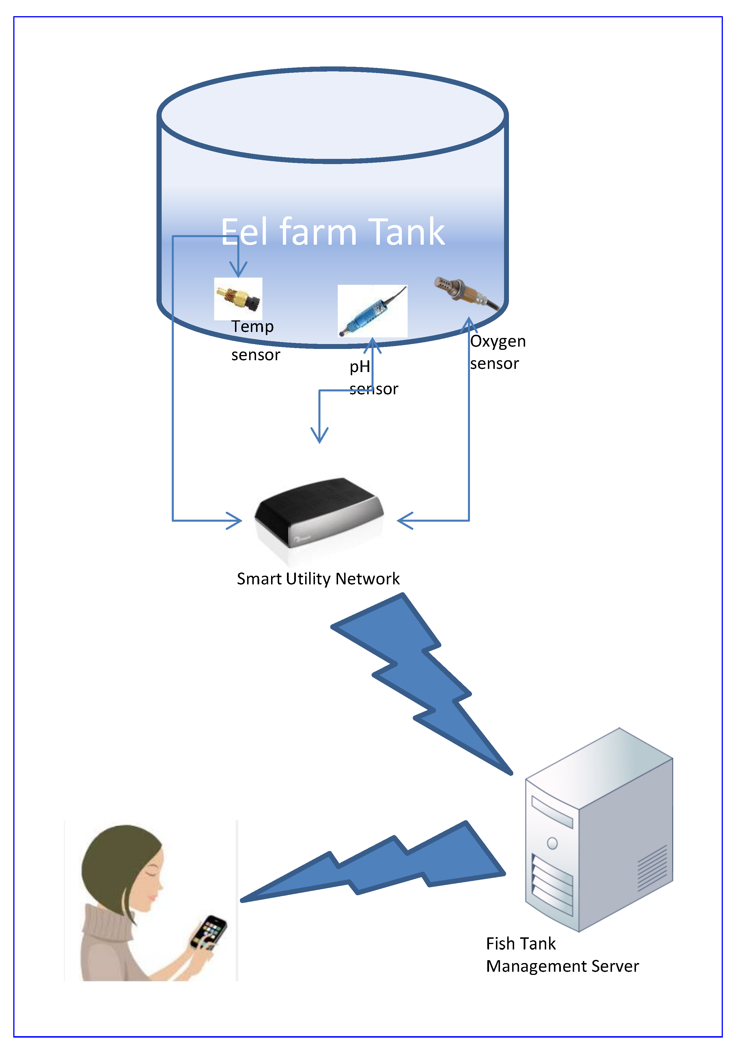
Smart farming is considered as an ultimate solution for rising global food requirement with growing population [22]. Traditional farming needs to counter new challenges with global climate changes in the form of extreme weather condition, heavy rainfall, scorching heat waves and storms, limited fresh water, etc. FAO strongly encourages and recommends that all farms (livestock, agriculture, fish farms, etc.) be equipped with modern tools and technologies. SK Telecom (Korean Telecom Company) has started a pilot project to develop an IoT-based Fish Farm Management System and their proposed system design is presented in Figure 1 [11]. Initially, they used the system for eel farms and later planned to test it on other species of fish. Their system utilizes a near field communications technology to observe key indicators including water temperature, pH and dissolved oxygen and enables farmers to use their smartphones for real-time monitoring and systematic management of the farms. In this IoT-based fish farm management system, three sensors are installed on each fish tank to measure water temperature, pH, and oxygen level. Sensor data are periodically collected with typical frequency of 2 and 6 h for young and grown fish, respectively. Conventional methods of water quality testing for its chemical and biological properties in laboratories are performed manually by collecting samples from different filed locations. Shareef et al. presented an IoT based decision support system for real time monitoring of fish ponds using wireless sensor network to measure physio-chemical properties of water and notify user via smart phone [23]. Daudi et al. developed a monitoring system for aquaculture based on wireless sensor networks to control water quality [24,25]. Various water parameters, e.g., temperature, oxygen, pH and water level, are collected via sensors and communicated to main server via ZigBee protocol. They collected data for six months to analyze sensors data, network and battery performance. They applied simple rule based scheme to control pump operation without any optimization. Similarly, ref. [26] developed a sensor based monitoring system for plants growing in hydroponics. User can remotely monitor the status of various parameters and send command to control the environment accordingly. Raju at al. proposed an embedded system (Raspberry Pi) based monitoring solution for aquaculture [27]. It continuously monitors the water quality through onboard sensors and the data are stored on cloud server for analysis. Server sends an auto-generated notification/alert message if any parameter value is found out of range. The proposed system does not support any control and optimization strategies. Chen et al. developed an automated monitoring system for fish farm aquaculture environment using embedded micro-controller MSP430 with various sensors attached for water quality assessment [28]. User can remotely monitor and control the fish farm environment using their mobile device through android application. Luna at al. developed a mobile robotic prototype to look after fish farm [29]. The robots has water multi-parameter node to collect various sensor measurements and food containers with fish feed. User can define a monitoring and feeding schedule for the robot via a client application and the robot will then automatically carry out those operations. Working of this system is dependent upon user defined schedule and does not include any optimization procedures. Besides fish farm water quality monitoring, several studied can be found in literature focusing directly on fish body health by attaching various sensors to it. Taniguchi et al. investigated the effect of fish body size on sensor communication in their proposed monitoring system [30]. They observed that, with increase in fish body size, data gathering ratio is significantly reduced in the network. Hongpin at al. performed several experiments to evaluate their prototype system for real time fish farm water quality monitoring [31]. They used ZigBee and GPRS protocols for communication between sensor nodes and central server. In this paper, they tried to improve communication reliability to support real time monitoring. Encinas at al. developed an Arduino based prototype for water quality monitoring using pH, temperature, and oxygen sensors [32]. Mobile and desktop interfaces were implemented to collect and visualize data. They considered system optimization via artificial intelligence algorithms in their future extension. Several similar fish farm monitoring systems have been proposed [12,13,14,15]. Most of these systems are designed to assist farmer by providing remote fish farm monitoring service. They do not consider resources optimization and control.

Libelium is a popular IoT platform provider and has developed software and hardware solutions for various domains with particular emphasis on smart cities and agriculture. Together with PHA Distribution Vietnam (PHA Distribution, one of the leading IoT and ICT distributors in Vietnam), they have installed an IoT based network in a fish farm located in Dong Thap Province using Libelium product [33]. Data on water oxygen, pH, temperature and conductivity are collected using sensor in real time for analysis. The project objective is to monitor water quality to prevent disease in fish for healthy food production.

To overcome fresh water requirement challenge for fish farms, various water treatment and recycling systems are used to purify farm water and thus reduce need for fresh water. Recirculation Aquaculture Systems (RAS) is a new eco-friendly and highly productive system especially design for closed fish farms. Various mechanical and biological filters are used to clean the farm water. Aqua Maof is a group of companies providing support and consultation in fish farming related technologies, equipment, machinery, marketing and various other services [34]. They have successfully built many indoor RAS, cage and land based fish farms in various countries.

A brief review on aquaculture is presented with focus on seaweed and fish monitoring and control [35]. The authors presented five different types of popular seaweed along with region wise global fish consumption. They also presented RAS architecture for typical fish farm having four tanks for monitoring and control. An artificial neural network based system is presented to predict water quality using historical data collected through sensors using remote wireless communication [36]. Lee [16] presents a review of anticipated benefits of developing an AI based software system for fish farm. They discussed prospectus application of various AI algorithms (ANN, Fuzzy logic and Expert system) for process automation of aquaculture industry. Smart Water—a fish farm software solution— is developed to store data concerning fish farm stock, orders, materials, employees and operations with an objective to provide quick access to required information for better decision making [17]. This application does not include any automated monitoring and control system and needs to be manually operated by users. Several IoT based solutions are deployed in fish farms located in China and Yuan et al. [37] provided a detailed evaluation scheme of selected installations using 40 different performance indicators. Zhang et al. [38] conducted a study to present the financial gain due to IoT application in fish farming in comparison with non-IoT fish farms and the difference is significant.

3. Proposed IoT based Fish Farm System

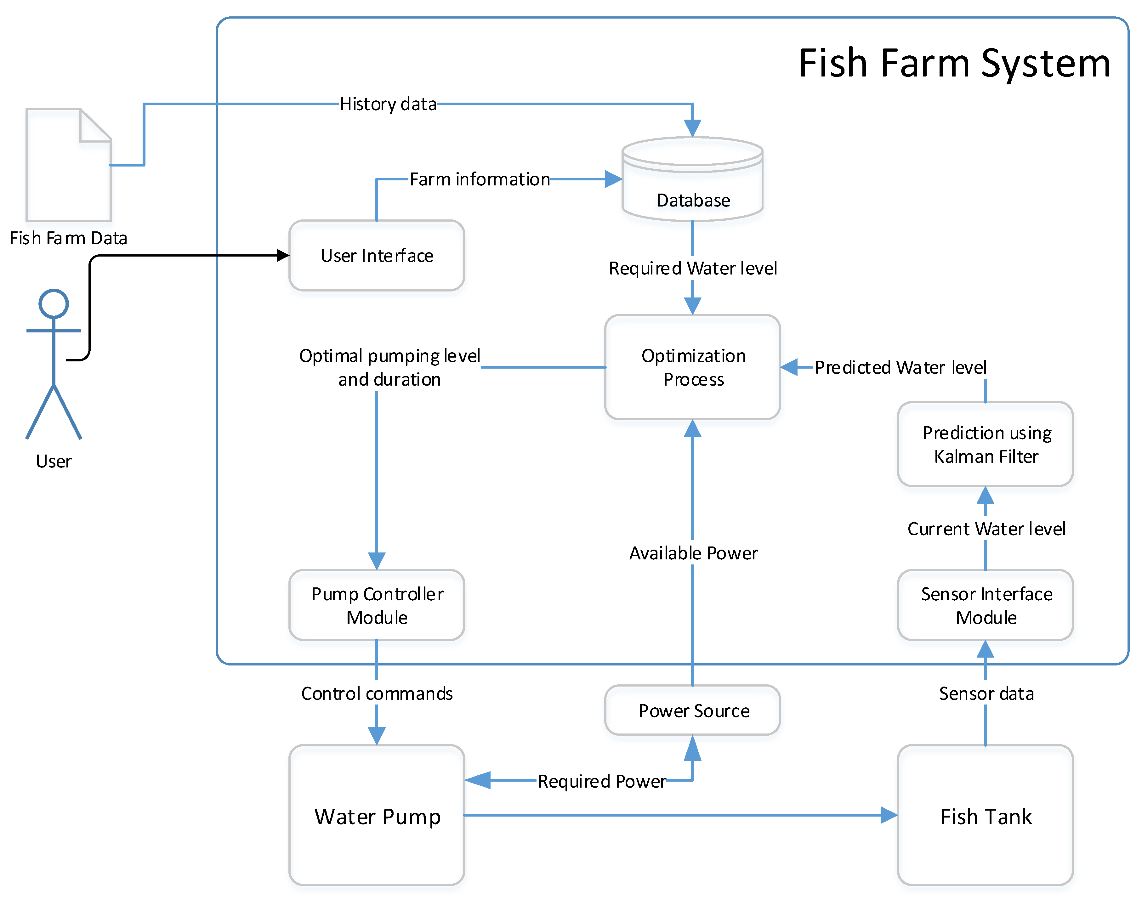
We developed a conceptual design for IoT based Fish Farm system (Figure 2). This design consider a closed environment of interest, i.e., a fish farm tank, which needs to be controlled by IoT based automated system for maintaining healthy environment for fish growth with efficient resource utilization. The whole process has four main steps. First, tank environment is monitored by collecting various data (e.g., temperature, oxygen level, water level, pH, etc.) through sensors. Sensor data provide current conditions in the tank. Second, prediction algorithm is applied to estimate future conditions using some historical data. This helps in adjusting/controlling the various parameters before the inside tank conditions worsen for the dwelling fish. Third, optimization techniques are required to compute optimal conditions by keeping in view the best settings for fish growth and system constraints, e.g., power. Finally, actuators levels are adjusted to control the tank water quality as per optimized settings for fish development. This helps in achieving best condition for fish growth with optimal resources utilization.

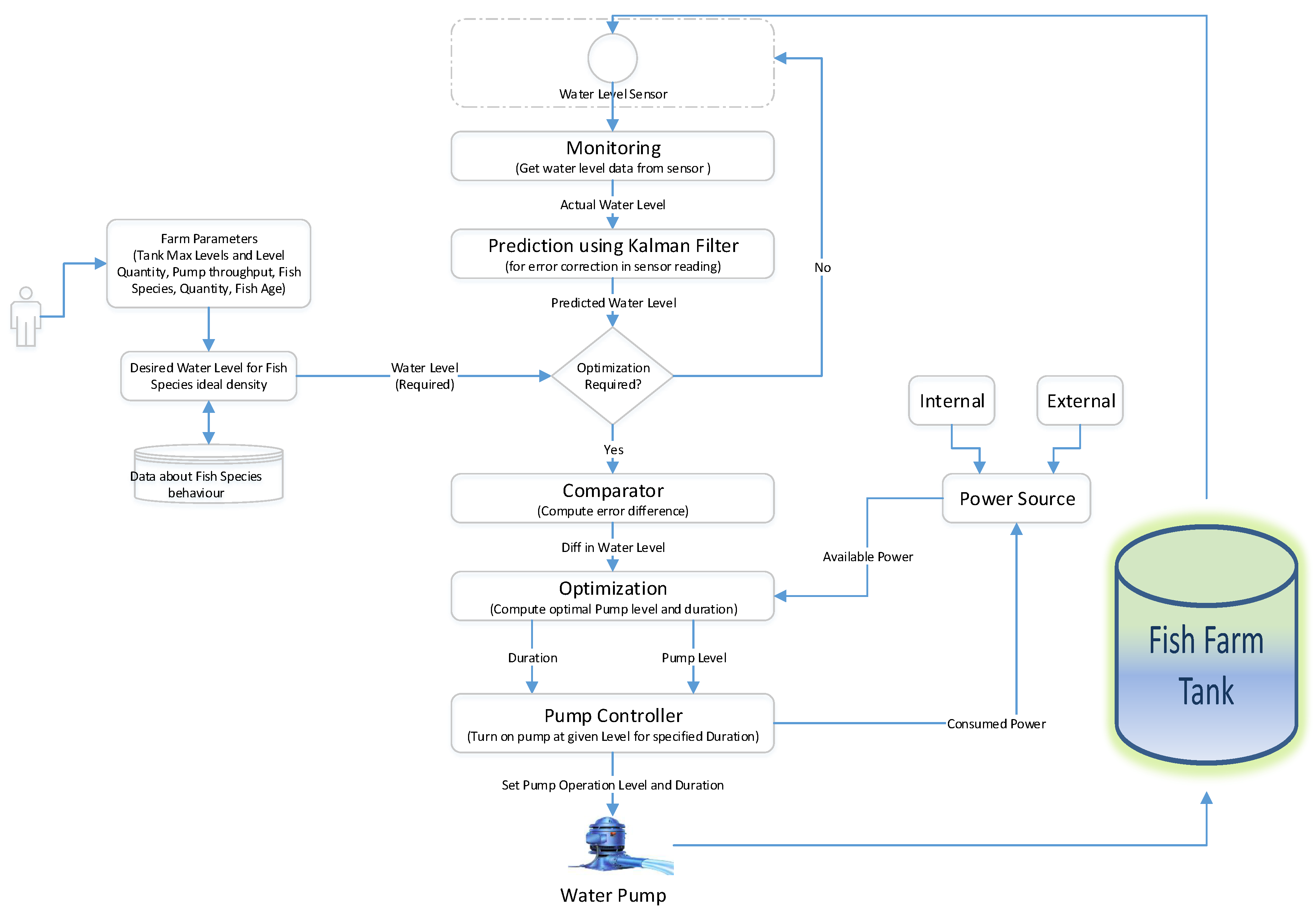
For the sake of demonstration, we consider a single parameter, i.e., water level maintenance in tank. However, the system design is flexible enough to serve as a foundation for a complete solution and include various other sensor data, e.g., temperature, oxygen, CO${}_2$ level, etc. The flow chart of the proposed system is shown in Figure 3. The process begins with reading current water level from sensors inside the tank. Kalman filter algorithm is applied to remove error in sensor reading and predict actual tank water level. If water level is below the desired range, then optimization is applied. During optimization, we try to compute optimal pumping level and duration to obtain desired water level inside the tank. Finally, these parameters are passed to pump controller module in order to send operation command to the pump.

The system has an internal database for storing data for comprehensive analysis of the system performance gain and optimal utilization of resources. An interface is also provided to users to specify system parameters, e.g., tank size, fish type, quantity, etc.

Usually, we have two kinds of water pumps, i.e., fixed and variable speed. Fixed speed pumps operate at a particular speed (although its effective flow rate may vary due to operating conditions) and consumes a fixed amount of energy. There is no mechanism in such pumps to increase/decrease its pumping speed. On the contrary, variable speed pumps have the ability to operate at different pumping levels to produce different flow rate as per user demand and requirement. Normally, higher pumping level consumes more energy as compared to lower pumping levels. Instead of using the common standard type induction motors, for these experiments, we consider permanent magnetic motors based variable speed pump. In fish farm environment, pump energy consumption can be reduced by lowering the pumping flow rate, but then we need to operate the pump for extra amount of time, e.g., if a pump requires to be operated with flow rate of 80 ${ft}^3$/min for 8 h daily, then operating the same pump with flow rate of 40 ${ft}^3$/min will require 16 h of operations on daily basis. Data recorded from actual experiments with permanent magnetic based variable speed pump manufactured by [39] shows that operating the pump with lower speed, even for extra 8 h daily (total 16 h), results in almost $63\%$ reduction in net power consumption which is indeed a significant savings.

Although maximum energy can be saved by operating the pump at lowest flow rate, there are some repercussions: (a) it will take more time to fill the tank, which is not desirable; and (b) this will reduce lifetime of the pump, as every pump ideally operates near its Best Efficiency Point (BEP), otherwise, pump performance and lifetime will be degraded [40]. BEP is the measure where pump performance is most effective and less likely to fail. Operating a pump at flow rate more than $40\%$ towards right or left of the BEP may damage the pump. Furthermore, besides flow rate, there are other factors which effects pump performance, e.g., pressure, head, etc.

3.1. Kalman Filter Formulation for Water Level Prediction

Often, data read from sensors have noise which not only affects their accuracy but also generates spikes in the data. Kalmans filter is a very elegant and lightweight algorithm to make intelligent guess about system real state using only the previous state (i.e., no need to keep all historical data), as shown in Figure 4. It is used for data smoothing when there is rapid variation (good for dynamic systems). It is good for predicting actual state of the system when there is uncertainty (make well educated guess). The best thing about this algorithm is its ability to quickly get to the stable state even if initial supposition about the system’s state is not so accurate. All magic is performed by the Kalmab’s gain (often denoted by K) which defines whether more preference shall be given to sensor reading or system’s internal predicted state to accurately estimate the real state of the system.

In this study, estimated water level is computed from water level sensor installed in tank which commonly have error in its readings. Thus, we use the Kalman filter algorithm in order to remove error in sensor readings and estimate actual water level. Let’s assume estimated water level at time t is $W_t$. Using estimated water level $W_t$, we can predict water level at next time stamp $t+1$, i.e., $W_{t+1}$, using Kalman filter algorithm. Step by step calculations are given below.

First, we calculate water level from previously estimated water level as below

$$W_{predicted}=A·W_{t-1}+B·u_t$$

where A is state transition matrix, B is control matrix, $W_{t-1}$ is previously calculated water level and $u_t$ is control vector. Next, predicted covariance factor can be updated as

$$P_{predicted}=A·P_{t-1}·A^T+Q$$

where $A^T$ is transpose of state transition matrix, $P_{t-1}$ is previously calculated covariance and Q is estimated error in the process. Then, we adjust the Kalman’s Gain K as

$$K=\frac{P_{predicted}·H^T}{H·P_{predicted}·H^T+R}$$

where H ($H^T$ is transpose of H) is observation matrix and R is estimated error in the measurements. Assuming current sensor’s reading for tank water level at time t is $z_t$, then Kalman filter predicted water level for current time interval becomes

$$W_t=W_{predicted}+K·\left(z_t-H·W_{predicted}\right)$$

Finally, we update the covariance factor for next iteration as below

$$P_t=\left(I-K·H\right)P_{predicted}$$

3.2. Formulation for Optimization

In this section, we present our model for resources optimization in smart fish farm. We have developed a model for single tank and the same can be extended for any number of tanks. Let us assume we have a fish tank having maximum capacity of V ${ft}^3$. The tank has a particular fish species with certain density that requires water level to be maintained with certain range all the time. We can express total capacity of water tank as $T_c=V$ ${ft}^3$. If volume of water per level is $W_p=w$ ${ft}^3$, then maximum number of water level in tank $T_m$ can be calculated as

$$T_m=L=\frac{V}{w}$$

Table 1. Description of notations used in formulation.

Notation	Description
$W_c$	Current water level in tank.
$W_d$	Desired water level in tank.
$T_c$	Maximum capacity of the tank
$W_p$	Volume of water per level.
$T_m$	Total number of levels in the tank.
$BEP$	Pump Best Efficiency Point
$P_f$	Flow rate of the pump
$P_d$	Pumping duration of the pump
$R(P_f,P_d)$	Energy required for pump operation for given flowrate and duration.
$E\left(x\right)$	Energy required for pumping flow rate x per unit time.
$\alpha$	Factor describing pump lower and upper limits around BEP.
$D_{min}$	Minimum operational duration of pump for delivering required amount of water.
$D_{max}$	Maximum operational duration of pump for delivering required amount of water.
G	Required amount of water.
$R_{min}$	Minimum energy required for pump to deliver required amount of water.
$R_{max}$	Maximum energy required for pump to deliver required amount of water.
${\beta }_1$	User set preference (weight) for pumping duration.
${\beta }_2$	User set preference (weight) for energy savings.

presents brief description of various notations used in this formulation.

Assume the current water level is $W_c=c$, and desired water level is $W_d=d$. Consider BEP of water pump is $BEP=Bf{t}^3$/min with alpha $\alpha =x$, so pump feasible operation flow rates $P_f$ shall be in range given below.

$$P_f\in [BEP-\alpha ,BEP+\alpha ]$$

Required amount of water is expressed as G can be calculated using following expression

$$G=(d-c)\times w{ft}^3$$

To deliver $Gf{t}^3$ of water, we can calculate operating duration of pump $P_d$ as below

$$P_d=\frac{G}{P_f}$$

where $P_f$ is the pump selected flow rate. Energy required to deliver $Gf{t}^3$ of water with pumping flow rate $P_f$ for duration $P_d$ can be calculated as below.

$$R(P_f,P_d)=E\left(P_f\right)\times P_d$$

where $E\left(x\right)$ denotes the amount of energy required for operating the pump with flow rate $P_f$ per unit time. $E\left(x\right)$ signifies the relationship between energy consumption and flow rate (we assume a linear positive relationship between the two).

If there is no restriction on pumping duration, then we can set pumping flow rate to its minimum, i.e., $P_f=BEP-\alpha$ (lowest flow rate), to save max energy. In practice, we cannot afford slow refilling all the time. Thus, we need to find some trade-off between pumping duration and flow rate. We can express pumping minimum and maximum duration as below

$$P_d\in \left[D_{min},D_{max}\right]$$

where

$$D_{min}=\frac{G}{max\left(P_f\right)}$$

$$D_{max}=\frac{G}{min\left(P_f\right)}$$

Similarly, minimum and maximum amount of energy required to deliver $Gf{t}^3$ of water can be computed as below:

$$R\in \left[R_{min},R_{max}\right]$$

where

$$R_{min}=E\left(min\left(P_f\right)\right)\times P_d$$

$$R_{max}=E\left(max\left(P_f\right)\right)\times P_d$$

User preference for time and energy savings is ${\beta }_1$ and ${\beta }_2$, respectively, where

$${\beta }_1+{\beta }_2=1$$

Values of ${\beta }_1$ and ${\beta }_2$ serves as control parameter and its values can be set adaptively as per the difference between current and desired water level using the following formula.

$${\beta }_1=\sqrt[1/3]{\frac{d-c}{d}}$$

(1)

$${\beta }_2=1-{\beta }_1$$

(2)

To assign reasonable weight to ${\beta }_1$ for smaller difference between desired and current water level, cube root is taken in above formula.

After above necessary definitions and formulation, we can now define our optimization function as below:

$$max\left({\beta }_1\times \left(1-{\left(\frac{P_d-D_{min}}{D_{max}-D_{min}}\right)}^2\right)+{\beta }_2\times \left(1-{\left(\frac{R-R_{min}}{R_{max}-R_{min}}\right)}^2\right)\right)\in [0,1]$$

(3)

i.e., we want to minimize the pumping duration $P_d$ to maximize our optimization function. Lower values of pumping flow rates $P_f$ will have increased values for resultant pumping duration $P_d$. Our goal is to have such a pumping flow rate $P_f$ which results in minimization of the subtraction part in the first component of our optimization formula. Thus, for maximizing objective function, we need pumping duration $P_d\to D_{min}$, which will make the subtraction part ${\left(\frac{P_d-D_{min}}{D_{max}-D_{min}}\right)}^2\to 0$ and we get max of ${\beta }_1$. The same holds true for energy consumption part. Constraints:

$$0\le W_c\le W_d\le L$$

$$0\le D_{min}\le P_d\le D_{max}$$

$$0\le R_{min}\le R\le R_{max}$$

3.3. Illustration of Optimization Scheme

Let us suppose our pump $BEP=60$ and $\alpha =20$, so we have feasible range for pump flow rate $=[60-20,60+20]=[40,80]$. Further assume the predicted current water level is 3 and desired optimized water level 4, and water per level equals 400 ${ft}^3$. Using adaptive formula for beta values calculation, we get

$${\beta }_1=\sqrt[1/3]{\frac{d-c}{d}}=\sqrt[1/3]{\frac{4-3}{4}}=\sqrt[1/3]{\frac{1}{4}}=0.62$$

For ${\beta }_2$

$${\beta }_2=1-{\beta }_1=1-0.62=0.37$$

Considering a permanent magnetic based variable speed pump, we get the following results given in

Table 2. Optimization value for sample pumping flow rate.

Pumping Flow Rate	Optimization Value
70	0.58
60	0.80
40	0.75

for optimization formula given in above section for three sample flow rates.

We can see that pump flow rate of 70 gives the worst results. Even for lowest pumping rate (i.e., 40), the optimization value is smaller than flow rate of 60, because flow rate of 40 takes too much time to complete desired filling. Actual optimal flow rate is expected to be somewhere around 60.

However, we observed through testing results that average pumping flow rate (23 ${ft}^3$/min) with proposed optimization scheme stays below the BEP of the pump, i.e., 40 ${ft}^3$/min. Data log inspection reveals that optimization is done so fast that difference in current and desired water level is very small. For these experiments, we consider effluent water rate as 5 ${ft}^3$/min. We read the data from tank sensors with time interval of one minute. Once desired water level in tank is reached, the system maintain desired water level in tank as optimization is done after every single minute in which water level can decrease maximum by 5 ${ft}^3$/min.

Table 3. Data log of tank water level for first 20 min.

Time (min)	Water Level ${\mathit{ft}}^3$	Optimized Pump Flow Rate ${\mathit{ft}}^3$/min
1	1979	25
2	1996	23
3	1998	23
4	2000	23
5	1997	23
6	2000	23
7	1999	23
8	1999	23
9	1998	23
10	1997	23
11	2002	22
12	2000	23
13	1999	23
14	1999	23
15	2003	22
16	2000	23
17	2001	22
18	2002	22
19	1998	23
20	1996	23

shows data log of tank water level for first 20 min. For low difference in current and desired water level, our adaptive formula results in very low values for ${\beta }_1$. Lowering ${\beta }_1$ results in higher value of ${\beta }_2$ which means more preference to energy savings. More energy can be saved with low pumping rates. The same can be observed from data log. At the beginning, when current water level in tank was 1979 ${ft}^3$, the difference between current and desired water level was high, resulting in higher values for ${\beta }_1$. Therefore, relatively higher pump flow rate was selected by optimization scheme, i.e., 25 ${ft}^3$/min. Soon afterwards, desired water level of 2000 ${ft}^3$ was achieved and then no significant drop in water level was observed. As the difference between current and desired water level is small, ${\beta }_1$ gets smaller weight. Consequently, optimization scheme gives more preference to energy savings by selecting lower pumping flow rates. This is why optimal scheme results in pumping rate of 22 or 23 ${ft}^3$/min, i.e., it stays below BEP of pump.

Continuous operation of water pump at very low flow rates is highly undesirable, therefore we need to revise optimization formula to address this issue.

3.4. Investigations for Improved Optimization Function

One possible solution could be having desired water level in a range, i.e., $[min,max]$. Perform optimization only when water level gets below the minimum level and adjust pumping duration and flow rate to set water level somewhere between $[min,max]$ such that optimization gain is maximum. Let us suppose, we choose our $min=2000$ and $max=2080$. Now, as tank water level goes below 2000, our optimization procedure will be activated to set target water level somewhere between 2000 and 2080 such that optimization gain is maximum. 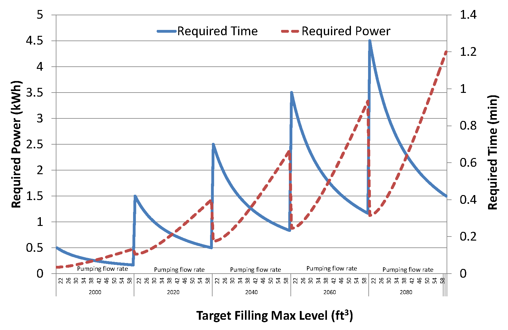Plotting the required time duration and energy for pumping with BEP 40 and alpha $\pm 20$, we get the graph shown in Figure 5. These calculations are made with tank current water level as 1990 $f{t}^3$. First, we consider target water level is to be 2000 and calculate required time and energy for varying pump flow rate between 20 and 60. Next, we consider target water level is to be 2020 and the same calculations are repeated for varying pump flow rate between 20 to 60. Its worth mentioning here that Figure 5 have dual x and y-axis. Primary y-axis shows the required power (kWh), whereas required pumping duration is expressed on secondary y-axis. Similarly, on x-axis, the values 2000, 2020, ..., 2080 show the selected target filling level and the values 22, 26, ..., 58 show pumping flow rate from 20 $f{t}^3$/min to 60 $f{t}^3$/min repeated for each selected target filling level. We can see that there is a gradual linear increase in the trend as we increase our target level. For a particular target level:

• Energy consumption is minimum and duration is maximum for starting flow rate of 20 $f{t}^3$/min.
• Moving from left to right, i.e., with increase in pumping flow rate, we can see energy consumption goes up and duration curve experience decline.

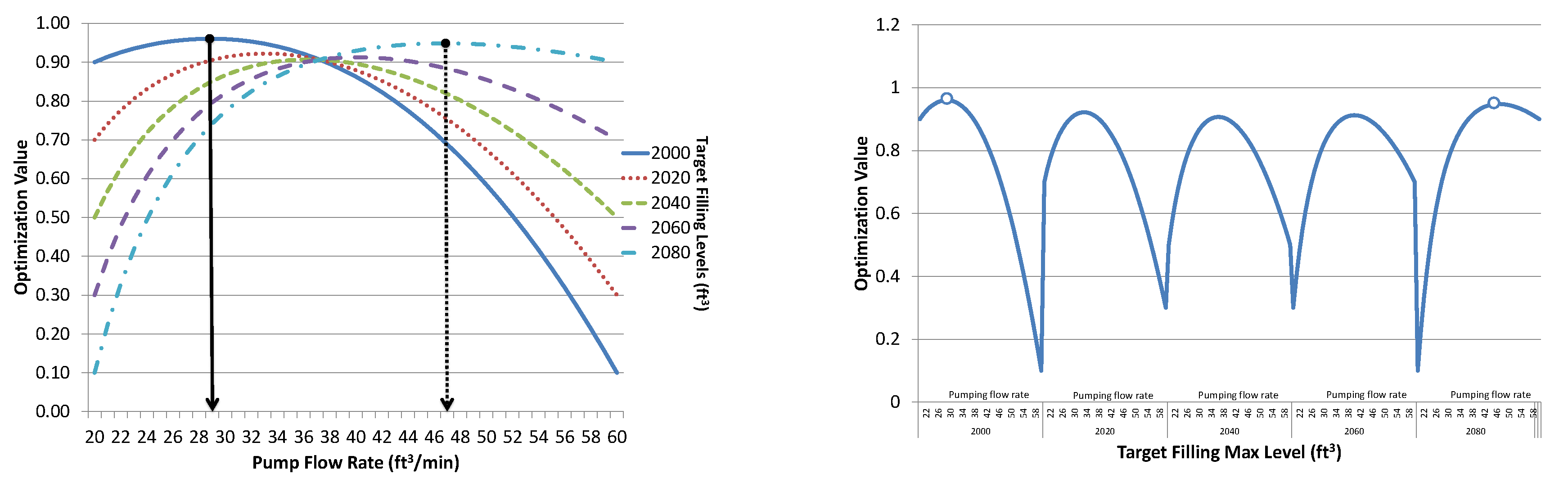
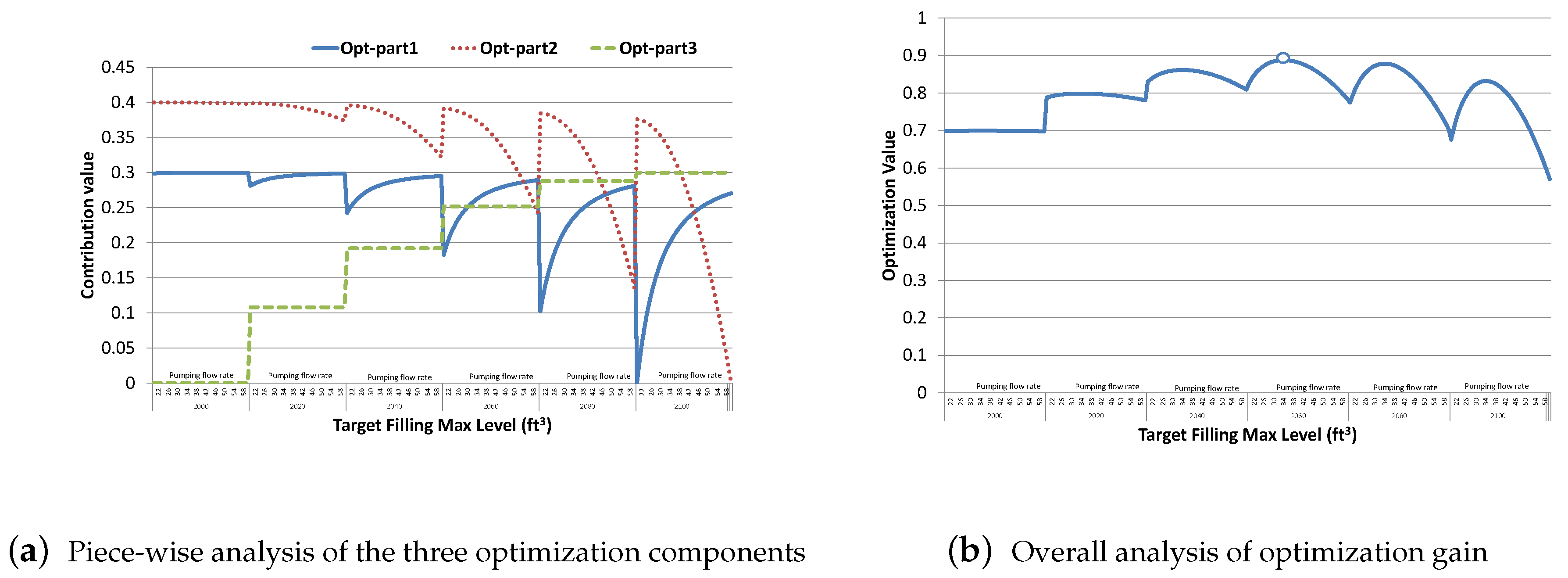
Next, we apply our optimization formula for each target level to find the optimal pumping rate and tank filling target level. Results are shown in Figure 6 (assuming current water level as 1990). Optimization value, expressed on primary y-axis of Figure 6, requires no unit information as this value indicates the fitness level of selected settings, i.e., settings resulting in optimization values close to 1 are desirable.

Two best optimal points can be seen in Figure 6a: (a) the first one is indicated with solid black vertical line dropping for dark blue curve representing target filling level as 2000 $f{t}^3$, i.e., our optimization scheme is preferring lowest filling target with low pump flow rate of 29 $f{t}^3$/min; and (b) the second highest optimal point (indicated with dotted black vertical line) is for the light blue curve representing target filling level as 2080 $f{t}^3$ with pump flow rate as 47 $f{t}^3$/min. Figure 6b shows the same results from a different angle which makes it clear that our optimization scheme is favoring the extreme target filling level, i.e., 2000 $f{t}^3$ and 2080 $f{t}^3$. This is not even considering the middle filling options because of low optimization gain. In a way, our optimization formula is favoring the extreme options (indicated with small circles in Figure 6b) for target filling level, i.e., either min or max which is against the spirit of optimization schemes. Optimization is all about finding the balance point and should normally prefer the middle ground and drift slightly towards left or right depending upon the conditions.

It seems that even having variable target filling options does not produce desired results. After careful analysis, we revised our proposed optimization formula to include a third component for considering tank target level filling such that the formula prefers more filling. The benefit of having higher target filling is that pump will operate for a while and then will remain OFF for a longer period. This is good for longevity of pump lifetime to have reduced pump ON/OFF sequence. Our modified optimization function is given below.

$$max\left({\beta }_1\times \left(1-{\left(\frac{P_d-D_{min}}{D_{max}-D_{min}}\right)}^2\right)+{\beta }_2\times \left(1-{\left(\frac{R-R_{min}}{R_{max}-R_{min}}\right)}^2\right)+{\beta }_3\times \left(1-{\left(\frac{Fil{l}_{max}-Fil{l}_{opt}}{Fil{l}_{max}-Fil{l}_{min}}\right)}^2\right)\right)\in [0,1]$$

(4)

where

$$Fil{l}_{min}\le Fil{l}_{opt}\le Fil{l}_{max}$$

and $D_{m}in$, $D_{m}ax$, $R_{m}in$ and $R_{m}ax$ are calculated locally for every target filling level.

Brief descriptions of the first two components (duration and energy) are given in earlier section. Here, we briefly explain the third component, i.e., tank target filling level. As stated earlier, to have effective optimization, we want to set tank target filling in a range $[min,max]$ and adjust pumping to set water level in between such that optimization gain is maximum. The third component in the formula serves the same objective and its contribution in optimization is controlled by parameter ${\beta }_3$. As $Fil{l}_{opt}\to Fil{l}_{max}$, the subtraction factor from 1 tends to zero and we get maximum part for the third component and vice versa.

3.5. Illustration and Verification of Revised Optimization Function

Now, our modified optimization formula has three components as given in Equation (4). Contribution of each component in overall optimization value can be adjusted and controlled by parameter beta such that

$${\beta }_1+{\beta }_2+{\beta }_3=1$$

For detailed analysis of variation in each component of the revised optimization formula, we performed some experiment to get better understanding and the results are presented in Figure 7. Similar to the optimization value, contribution value expressed on primary y-axis of Figure 7 shows the contribution made by each part to overall optimization value and requires no unit information as the maximum value for each part is controlled by respective beta values and the total sum of all parts can never exceed 1.

Assume the current water level is 1990 $f{t}^3$ and tank min and max target filling level to be $[2000,2100]$. Pump flow rate can vary between 20 and 60 $f{t}^3$/min and beta values settings were as follows: ${\beta }_1=0.3$, ${\beta }_2=0.4$, and ${\beta }_3=0.3$. Results given in Figure 7a show the variation in component-wise contribution to overall optimization value for varying tank maximum filling level and pump flow rates. To better understand the results presented in Figure 7a, optimization formula given in Equation 4 can be written as below.

$$max\left({\beta }_1\times Op{t}_{part1}+{\beta }_2\times Op{t}_{part2}+{\beta }_3\times Op{t}_{part3}\right)\in [0,1]$$

(5)

$Op{t}_{part1}$ is about minimizing pumping duration, $Op{t}_{part2}$ is about minimizing energy consumption and $Op{t}_{part3}$ is about maximizing tank target filling level. For a particular target filling level, pump flow rate increases from left to right (20–60 $f{t}^3$/min) and $Op{t}_{part1}$ (Blue line) is polynomially increasing, i.e., it prefers higher pump flow rates to have reduced pumping duration. $Op{t}_{part2}$ (Red line) is polynomially decreasing, i.e., it prefers low pump flow rates to have reduced energy consumption. Previously, there was a gradual increase in pumping duration and energy consumption with increase in target filling level, as shown in Figure 5, but here we can observe that $Op{t}_{part1}$ and $Op{t}_{part2}$ follow the same pattern for every particular target filling. This is due to the scaling by the beta values in the revised optimization formula. With increase in target filling level, there is a gradual increase in $Op{t}_{part3}$ (Green line) which is about maximizing tank target filling level. In other words, $Op{t}_{part3}$ is contributing more for higher values of tank maximum target level. After analysis of individual component contribution, we now see the overall optimization gain by the modified optimization formula, as shown in Figure 7b.

Comparing results in Figure 7b with our previous results shown in Figure 6b, we can see that modified optimization formula has improved the results as expected. The maximum optimization point (indicated with a small circle) can be seen towards the end of curve representing target filling level as 2100 $f{t}^3$, i.e., our optimization scheme is preferring highest filling target with pump flow rate 35 $f{t}^3$/min. Despite this improvement, the formula seems to have a problem, as it gives maximum preference to the highest filling level in a way that it seems we would not consider lower filling levels as an option. This problem is due to the fact that, for $Op{t}_{part1}$ and $Op{t}_{part2}$, we are considering the local min–max duration and power consumption. This problem was resolved simply by considering global min–max for duration and power consumption. Figure 8a shows the variation in component-wise contribution with global min–max duration and energy consumption. As opposed to previous results, here we can observe that $Op{t}_{part1}$ and $Op{t}_{part2}$ do not follow the same pattern for every particular target filling. With increase in target filling level, there is a gradual variation in pumping duration and energy consumption. For lower target filling level, the first two components (duration and energy) are contributing the maximum but the third component (tank filling) is very low. With increase in tank filling level, the third component $Op{t}_{part3}$ starts contributing more and more but duration and energy components experience many variations in their contribution values. For example, with tank target filling level 2100, $Op{t}_{part3}$ is contributing maximum, whereas $Op{t}_{part1}$ experience gradual increase from low to high pump flow rates, i.e., it prefers maximum flow rate to reduce pumping duration. Conversely, $Op{t}_{part2}$ experiences gradual decrease from low to high pump flow rates, i.e., it prefers minimum flow rates to save maximum energy.

Results of overall optimization value is given is Figure 8b. Thus, by considering the global min–max values for duration and energy, we can see that the best optimal point is now somewhere in the middle (indicated with a small circle) representing target filling level as 2060 $f{t}^3$, i.e., our optimization scheme prefers an average filling target with pump flow rate 34. Furthermore, with changing current water level in the tank and beta values, the optimal point will drift toward left or right accordingly. For the sake of illustration, we take three different set of parameters having different sets of beta values as given in

Table 4. Beta values set for testing optimization function.

S. No.	Beta 1	Beta 2	Beta 3	Description
Set 1	0.3	0.4	0.3	All components (i.e., pumping duration, energy, target refilling) are given almost equal weights.
Set 2	0.5	0.4	0.1	Pumping duration is given highest weight, i.e., minimum pumping duration is highly desired.
Set 3	0.1	0.4	0.5	Tank target filling level is given highest weight, i.e., maximum tank refilling is highly desired.

. Current water level is assumed to be 1990 $f{t}^3$.

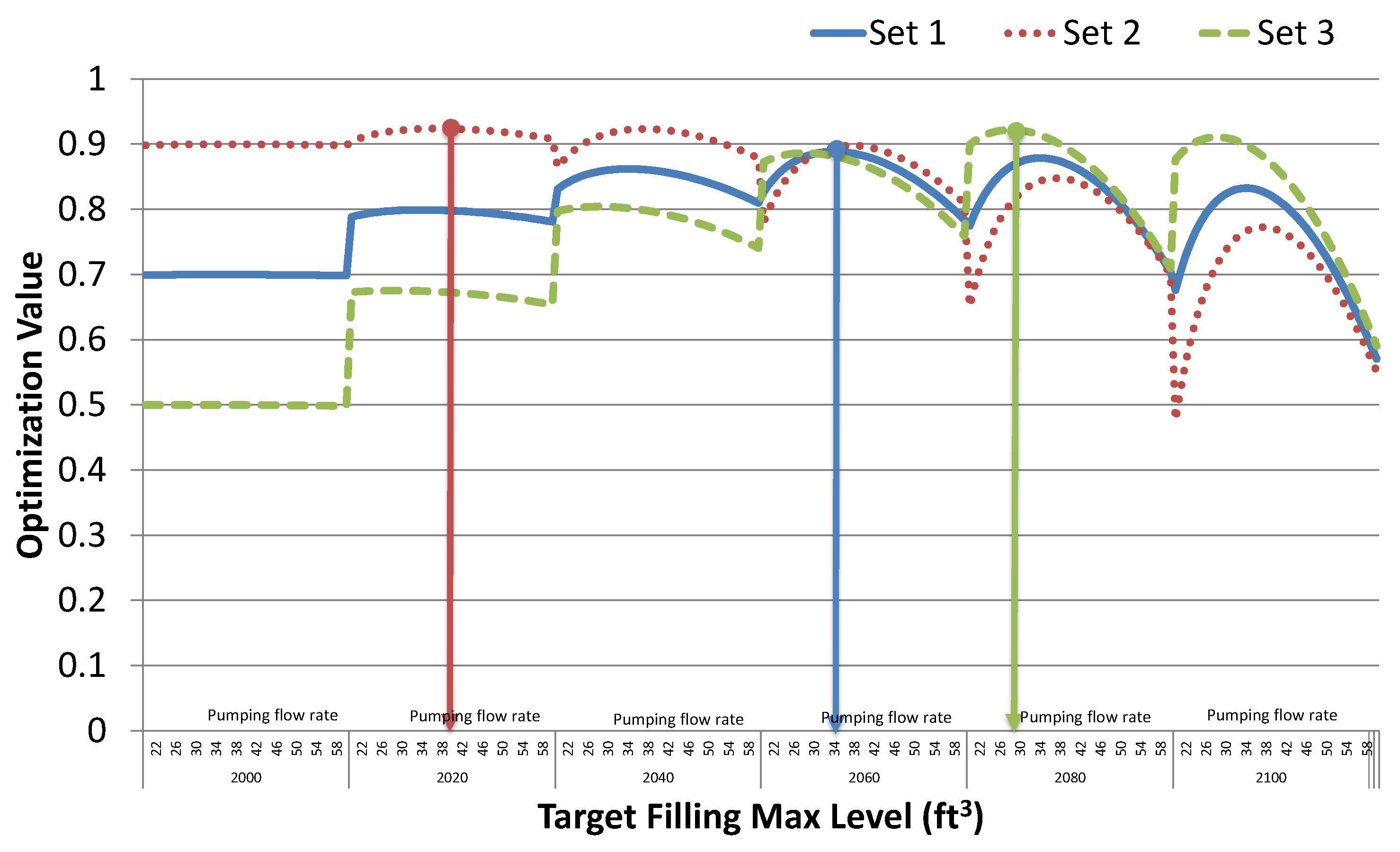
Optimization results for selected beta set values are given in Figure 9. Set 1 assigns almost equal weights to all three factors and its results stands in the middle of the other two sets with best optimal point for tank target filling level as 2060 $f{t}^3$ and pump flow rate as 34 $f{t}^3$/min. Set 2 gives more preference to time (pump duration) savings and therefore its best optimal point sets at tank target filling level as 2020 $f{t}^3$ with pump flow rate as 37 $f{t}^3$/min. Set 3 gives preference to higher tank filling to reduce pump ON/OFF sequence and therefore its best optimal point sets at tank target filling level as 2080 $f{t}^3$ with pump flow rate as 28 $f{t}^3$/min. These results confirms that our revised optimization is working as desired.

3.6. Alternate Schemes for Comparative Analysis

For comparison, we consider two alternate approaches that represen the two extremes. Brief descriptions of the approaches are given below:

Pumping with Min. flow rate: This approach selects the minimum tank target refilling level and operates the pump with minimum flow rate to save maximum energy as pump operating at lower rate consumes less energy. Of course, this will result in higher delay in tank refilling and pump will operate for longer period of time.

Pumping with Max. flow rate: This approach selects the maximum tank target refilling level and operates the pump with maximum flow rate to have minimum tank filling time but this will consume more energy as pump operating at higher flow rate consumes more energy. With maximum flow rates, we need to operate pump for a shorter period of time.

4. Experimental Design and Results

The proposed system has three main modules as shown in Figure 10. Fish farm system is the central component where different procedures are applied to ensure desired water level inside the tank with low energy consumption. It takes input from fish tank sensors and sends output to control pump operation level and duration. Power source represents the actual power source and our objective is optimal utilization of power. In these experiments, we have used two separate emulating modules to mimic operation and behavior of fish tank and water pump. Fish tank emulator is an independent module to emulate tank environment. Water pump emulator module is for emulating variable speed water pump operations. These experiments are conducted by considering a permanent magnetic motor based variable speed pump, i.e., IntelliFlo Variable Speed pump manufactured by Pentair Model #11018, with 230 operating voltage, full load 16 amps and 3 HP. This pump can be operated at various speed levels, i.e., 750–3450 RPM, producing different flow rates. Similarly, for water level measurement, we consider the typical water sensor module manufactured by Geekria, operating voltage 3–5 V DC, operating current less than 20 mA. This sensor generates analog output at various voltage level typically from 0 v to 1.88 V, indicating corresponding water level 0 cm to 4.8 cm, depending on how much the sensor is immersed in water.

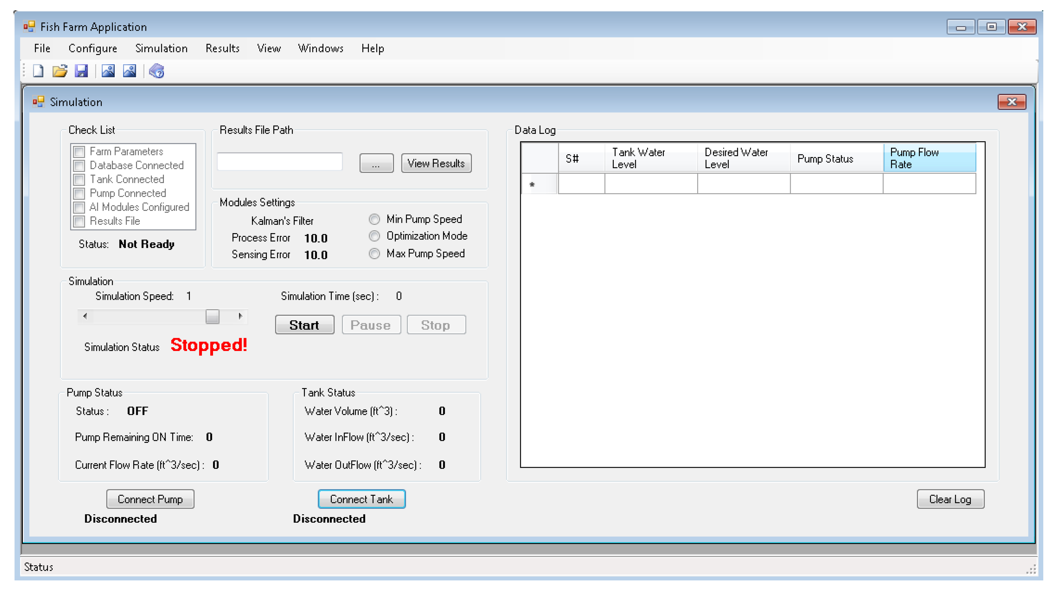
Fish farm main application was developed in Visual Studio C#. Figure 11 shows its main simulation interface window. Before starting the simulation process, this application needs several settings and configuration as given in check list. When check list is ready, the simulation can be initiated, otherwise appropriate error messages will be displayed instructing the user to do necessary settings. Once simulation is started, it gets sensor reading data from tank emulator process via windows communication foundation (WCF) service. Kalman filter algorithm is applied for error removal. Afterwards, optimization is performed to calculate optimal pump flow rate and duration which is then sent to pump emulator process via WCF service.

Next, we present detailed discussion on our experimental settings and results. For clarity, we present our results in two phases. Phase 1 is about the tuning of our prediction part of simulation setup using Kalman filter algorithm. In Phase 2, we present our findings during optimization process for energy consumption and pumping duration.

4.1. Analysis of Prediction Part Based on Kalman Filter

During phase 1, we tried two different approaches of Kalman filter implementation. First approach was based on internal estimation of water level and comparing the estimated water level with sensor reading to predict actual water level in the tank. Due to some internal settings/synchronization issues, results of our first implementation were not so accurate. Therefore, we tried a different approach while focusing on producing smoothing effect to remove error in sensor readings which gives us much better results.

Table 5. Parameter settings for analysis of Kalman filter algorithm.

Parameter	Value/Range
Desired Water Level in Tank	2000
Error rate in Sensor reading	± 10
Effluent Water Rate	5
Pump ($B,\alpha$)	(40, ±20)

presents the parameters settings for the Kalman filter algorithm used for these experiments.

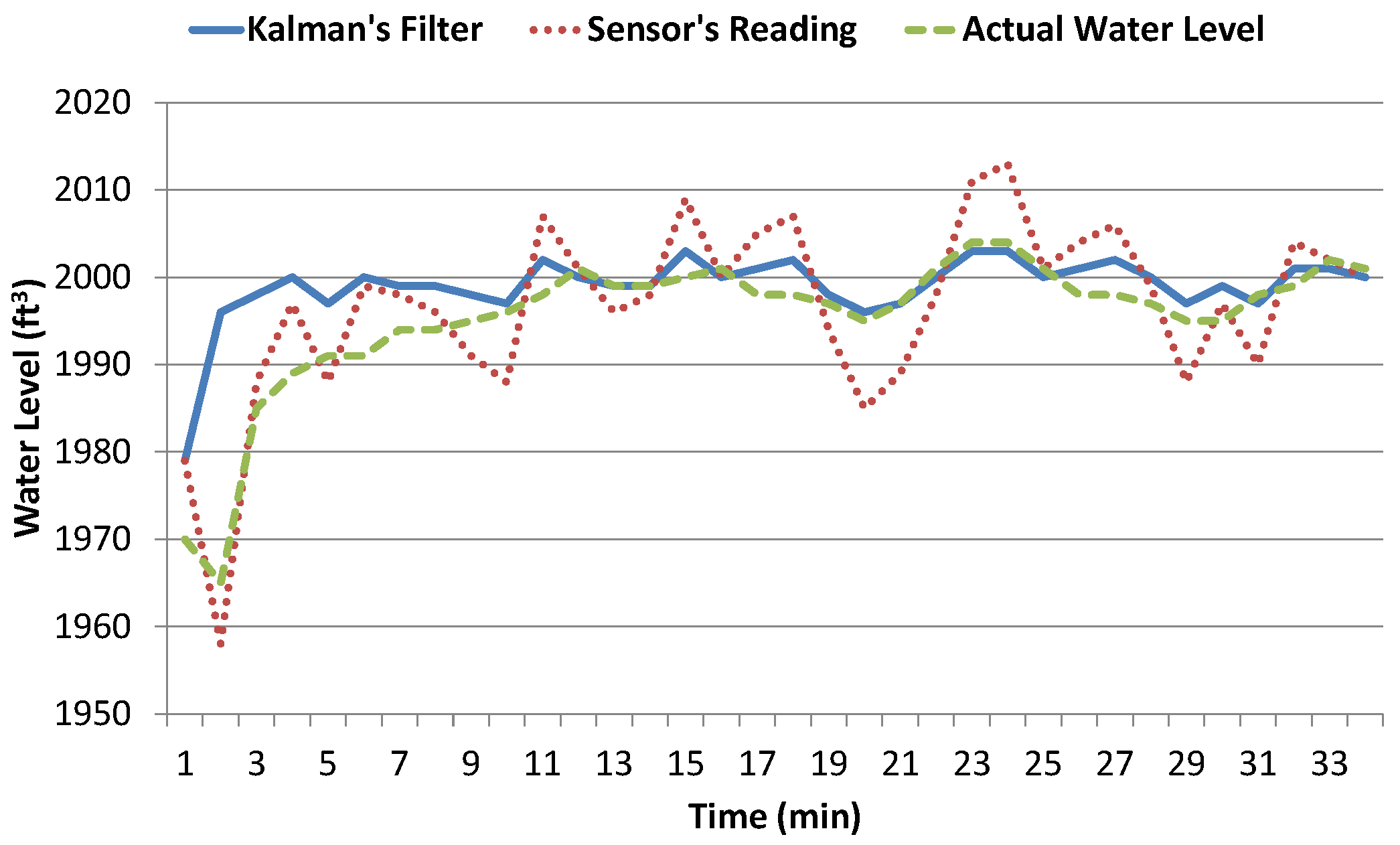
In these experiments, our objective was to maintain water level at 2000 ${ft}^3$ inside the tank but our initial results were able to maintain water level around 1995 ${ft}^3$ on average. This was rectified by adjusting the target water level for optimization, i.e., adding effluent water rate to desired water level to compensate for out flow. In other words, our effective desired water level is the summation of actual desired water level and effluent water flow rate. By making this adjustment, we can see that the system is able to achieve desired water level and it stays around 2000 ${ft}^3$, as shown in Figure 12. In first 10 min, Kalman filter results are deviated from actual water level but later it gets stabilized and was able to accurately remove error in sensor readings. Relative accuracy of Kalman filter results is $1.94$ in terms of Root mean square error (RMSE) when compared to actual water level. However, RMSE for sensor readings is very high, i.e., $5.26$. This manifests the utility of Kalman filter algorithm in our proposed system to accurately estimate contextual environment by removing error in sensors readings.

4.2. Analysis of Optimization Part

Our proposed optimization formula has three parts, as given in Equation (4). Contribution by each part to overall optimization value is controlled by beta values which are set adaptively. As stated earlier, pumping flow rate can be selected anywhere within $\left[BEP-\alpha ,BEP+\alpha \right]$. Optimization approach tries to find a balancing flow rate to have minimum power consumption with acceptable delay in tank refilling by selecting appropriate target filling level.

Before presenting power consumption and pumping duration results, we first look at how the three schemes perform in maintaining desired water level inside the tank. Figure 13 shows that all three schemes nicely maintain the minimum desired water level inside the tank, i.e., 2000 ${ft}^3$. These results indicate that there is no significant difference in three schemes as far as maintaining desired water level inside the tank is concerned and all of the them are good enough to achieve desired water level. Next, we compare their performance in terms of resource utilization.

Through optimization, we tried to find a tradeoff between the contradictory requirements, i.e., minimizing energy consumption with optimal tank refilling time. We want to have low energy consumption which compels us to operate pump with lower pumping rate but this will result in increase in pumping duration, i.e., slow tank refilling which is also not desirable. Our optimization formula helps us finding the best optimal pumping rate and maintains a balance between energy consumption and pumping duration by appropriately selecting tank target filling level.

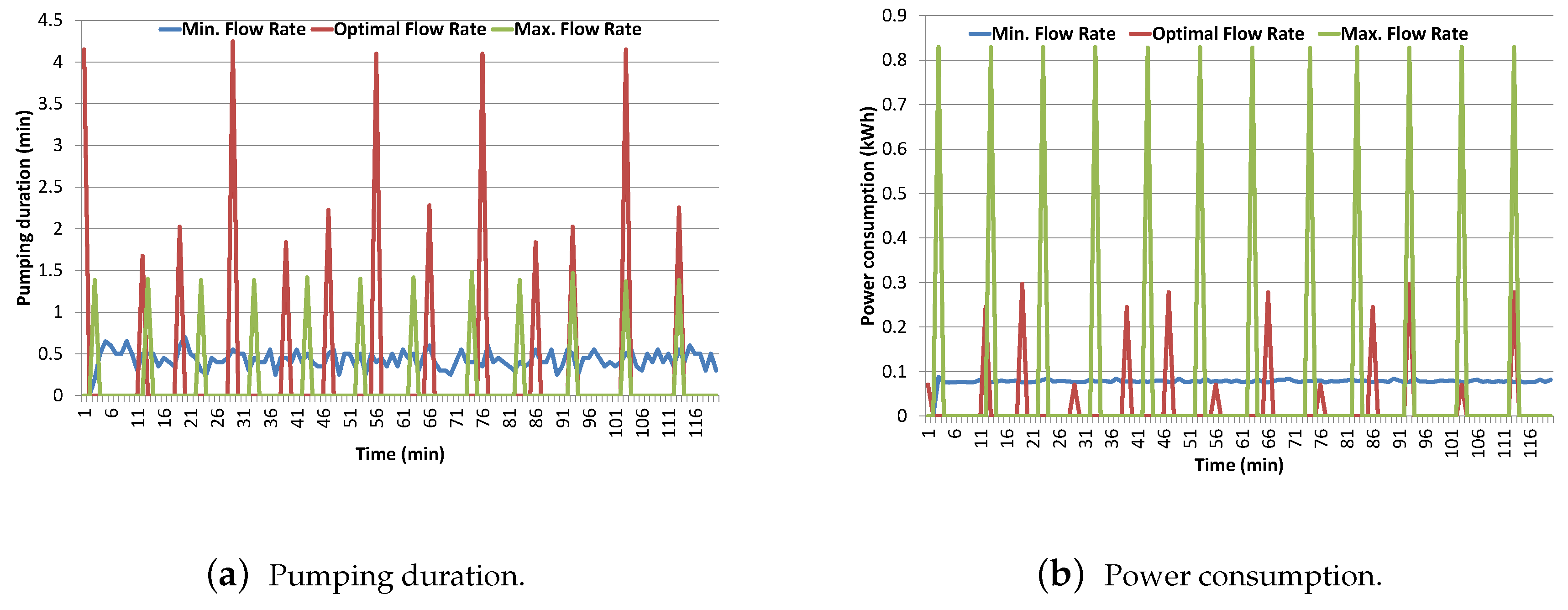
Figure 14 shows results comparison of pumping duration and power consumption for the three schemes. Pumping with maximum flow rate results in lower pumping duration at the cost of higher energy consumption as expected, i.e., $164.32$ W·h (on average), whereas optimal scheme energy consumption is very low, i.e., $41.62$ W·h (on average). On the other hand, pumping with minimum flow rate also results in high energy consumption, i.e., $153.25$ W·h (on average) due to continuous operation of the pump for short durations. In terms of pumping duration, minimum flow rate scheme takes too much time and its total pumping time is 51.2 min because it take too much time to fill the tank with lowest flow rate, whereas total pumping time of maximum flow rate scheme is the minimum (i.e., 16.86 min) as it can quickly fill the tank. Optimal scheme intelligently select appropriate target filling level and pumping flow rate to have minimum energy consumption with optimal pumping duration. The results shows that optimal scheme is able to achieve the best results in energy consumption (i.e., total $2.51$ kWh) as compared to the other two schemes. At the same time, total pumping duration for optimal scheme is also less than the minimum flow rate scheme (i.e., 36.92 min). Summary of the comparative analysis is given in

Table 6. Summary of the comparative analysis.

Parameters	Min. Flow Rate	Optimal Flow Rate	Max. Flow Rate
Pumping flow rate ( ${ft}^3$/min)	20	31.38 (avg.)	60
Selected target filling level ( ${ft}^3$)	2000	2075 (avg.)	2080
Total pumping duration (min)	51.2	36.92	16.86
Total energy consumption ($kWh$)	9.27	2.52	9.94

. Thus, through optimization scheme, we are able to obtain significant reduction in energy consumption relative to pumping with maximum and minimum flow rate schemes and reduction in pumping duration relative to minimum flow rate scheme.

5. Conclusions and Future Work

This paper presents a detailed study of the proposed optimization scheme for maintaining desired water level fish farm tank with minimum energy consumption by optimal selection of pumping flow rate and target filling levels. We have proposed a conceptual design for an IoT based solution for automation of fish farm activity. Proposed design can ensure maintenance of desired water level inside the tank for healthy fish production with optimal resource utilization. In this paper, we consider a single parameter, i.e., optimized water level maintenance in tank with minimum power consumption by controlling pump operation. We have developed an optimization scheme to achieve a trade-off between pumping duration and flow rate through selection of optimized water level. Comprehensive formulation is done for optimization with detailed analysis. We have used Kalman filter algorithm to remove noise/error in sensor readings. We observed through simulation results that optimization scheme can achieve significant reduction in energy consumption as compared pumping with maximum and minimum flow rate schemes and reduction in pumping duration relative to minimum flow rate scheme. The system is flexible enough to serve as a foundation for a complete solution and include various other sensor data, e.g., temperature, oxygen, CO${}_2$ level, etc. In the future, we will extend this work by considering other parameters for optimization along with detailed analysis to develop an automated system for smart fish farms to ensure healthy and productive environment for fish growth and development with optimal resources utilization.