1. Introduction
One of the major side effects of chronic kidney disease (CKD) is the reduced ability to produce endogenous erythropoietin (EPO), which is a hormone that regulates the production of red blood cells in the body. When the natural production of EPO drops significantly, these patients suffer from a condition called anemia, which is characterized by a reduced mass of red blood cells and hemoglobin level. Recombinant human erythropoietin has become the standard for treating anemia in chronic kidney disease [
1]. Recently, optimization of the EPO dosage has been considered to achieve reduced deviation of patient hemoglobin levels from a normal range (zone), while also reducing drug use and expense [
2].
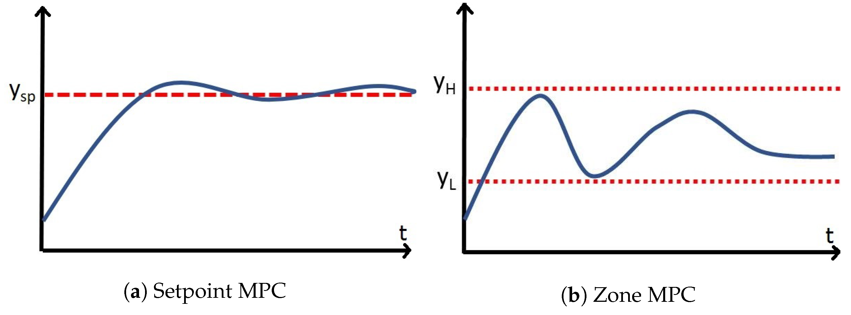
Zone model predictive controllers have become a popular area of research in the biomedical field [
3]. They have been used successfully in clinical trials in the control of blood glucose in Type 1 Diabetes Mellitus [
4,
5]. They have gained significant popularity over set-point tracking model predictive control (MPC) for biomedical applications due to their ability to reject sensor noise, and maintain a higher degree of stability in the presence of large plant–model mismatch [
6]. They also seem more appropriate for these applications as many of them do not have a target state, but rather a target zone.
The EPO dosing algorithms that have been developed and tested previously are open-loop devices. The patient will typically have their blood labs completed once every 2–4 weeks, and the EPO dose will be optimized for the time period in between sampling times. The EPO medications are approved manually by a clinician and administered during regular dialysis. It has been recognized by the clinical community that, while low Hb level leads to anemia, too high Hb levels can increase the risk of mortality for the patient [
7]. Hence, effective methods are needed to determine the appropriate dose of EPO to maintain the target Hb level.
To develop an automatic decision support system and achieve effective anemia management, some of the first published papers on the use of advanced process control in CKD utilize set-point tracking MPC combined with neural network hemoglobin response modeling and report promising results in clinical trials [
8,
9,
10]. The MPC algorithm in this case was an L1-Norm of the state deviation from the target. In another case [
11], a pharmacokinetic and pharmacodynamic model was used to describe the patient’s hemoglobin response and then designed controllers based on Quantitative Feedback Theory. In the small pilot study, these researchers also showed promising results. Modeling of hemoglobin response to EPO administration was also done under uncertainty via a recent method called semi-blind Robust Identification [
12]. The work presented in this paper differs significantly from these researchers. One of the more challenging aspects of hemoglobin control is the time-varying nature of the patient’s system dynamics. Patient’s can become EPO resistant [
13], as well as have their health improve drastically, if endogenous EPO production increases [
14]. To address the time-varying nature of the hemoglobin response, constrained recursive system identification is used. There exists a great deal of uncertainty in the model parameters, and the system is often subjected to acute disturbances, such as infection [
15] and blood loss [
16].
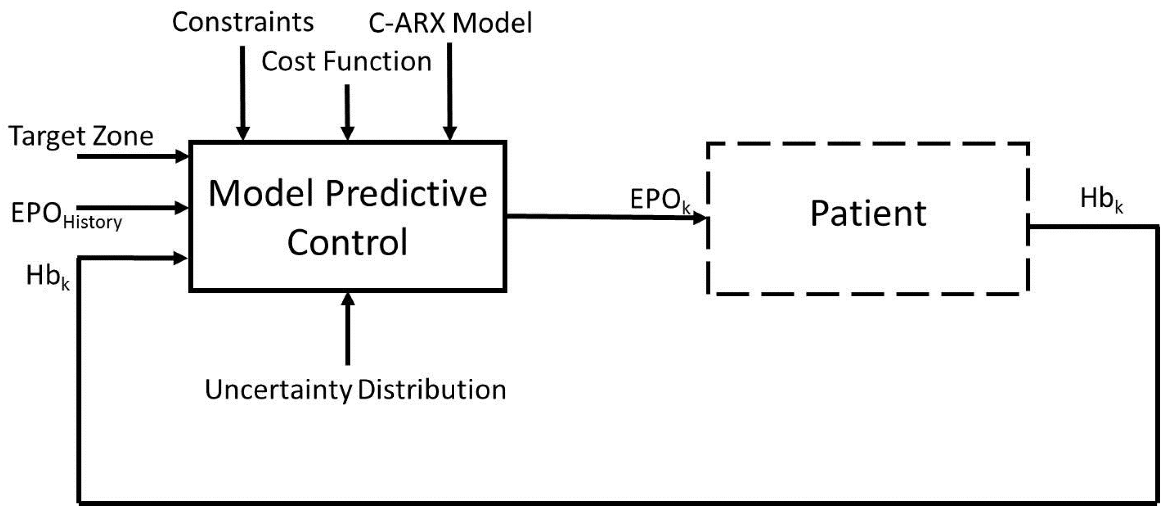
The aim of this work is to develop an advanced control system to calculate optimal EPO dosages for anemia patients, while considering process uncertainty in the control method. The overall block diagram of the control system is presented in
Figure 1. The method uses an autoregressive with exogenous inputs (ARX) model with a model predictive controller. To address the process uncertainty, it is represented in the form of different scenarios and further utilized within a model predictive control formulation, with the use of Conditional Value at Risk (CVaR) technique. CVaR was introduced by Rockafellar and Uryasev and is widely used in the finance industry [
17]. CVaR is a popular tool used in many risk management applications. For example, it has been shown to work well in heating, ventilation and air conditioning control systems [
18]; portfolio/asset optimization [
19]; and quantifying flood damage [
20]. However, it has been studied in very few applications related to model predictive control. The existing methods for model predictive control under uncertainty mostly include robust MPC [
21] and stochastic MPC based methods [
22]. The two methods address the worst-case performance and the expected performance, respectively. CVaR is a method that addresses both of these criteria. In addition, CVaR provides an effective convex approximation of a probabilistic constraint used in stochastic MPC. Thus, in this paper, the applications of CVaR for handling both risk averse performance and the probabilistic constraint are studied.
The rest of the paper is organized as follows.
Section 2 presents the hemoglobin response modeling through constrained optimization. Deterministic set-point and zone model predictive control algorithms are introduced in
Section 3, for comparison purposes to the CVaR methods introduced later. An overview of Conditional Value at Risk in general is introduced in
Section 4, which is a technique for addressing uncertainty. A set-point tracking model predictive controller using CVaR constraints on the upper and lower zone boundaries is then introduced in
Section 5 and later compared to the set-point tracking MPC. A second controller, a zone-tracking model predictive controller using CVaR directly in the cost function, is introduced in
Section 6 and later compared to the zone-tracking model predictive controller. In
Section 7, the controllers are tested in computer simulations. The experimental designs are outlined for a simple ARX model based simulator as well as for a physiological model based simulator, using both Gaussian and uniform uncertainty distributions.
Section 8 concludes the paper.
2. Hemoglobin Response Modeling
The system model used in the following derivations has an ARX model structure. This kind of model is one type that can be estimated through classic System Identification methods. The goal of System Identification is to map the response of a system’s output, to that of its input. The internal dynamics of the system are not known or estimated. This type of modeling is also referred to as black box modeling. In this work, the model parameters are obtained through constrained optimization. The model uses a weekly sampling time (
week), the last Hb measurement
, and several past EPO doses
(eight-week history of dosages in this work), to predict the future Hb measurement. The order of the
polynomial is 8 and was determined empirically [
23]. The order of the
polynomial in the model is set to 1. Using a higher order for the
polynomial may lead to inaccuracies in the model estimation and predictions because of the large amount of measurement error, mixed with the infrequent measurements typically used in the medical field. It is possible that, with more accurate measurements, a larger number of
parameters could yield better modeling results, but this work does not address this aspect.
Iron is necessary for the creation of red blood cells, but the effect of iron levels in the patient are ignored in this model. It is assumed that, if the treating clinician were to maintain stable and adequate iron levels within the patient, the response of the hemoglobin should be mostly related to the administration of EPO, and not related to fluctuating or low values of iron within the patient. If a patient were to have low iron levels, they will likely become EPO resistant which could effect the quality of the current model, should the change (from adequate to low levels) occur quickly. Future work should try to include the iron dynamics within the model, as there certainly are some dynamic interactions between these two systems.
The ARX model structure that maps the EPO administration events to the hemoglobin concentration is
where the input
u represents the EPO doses divided by 5000 international unit (IU), and
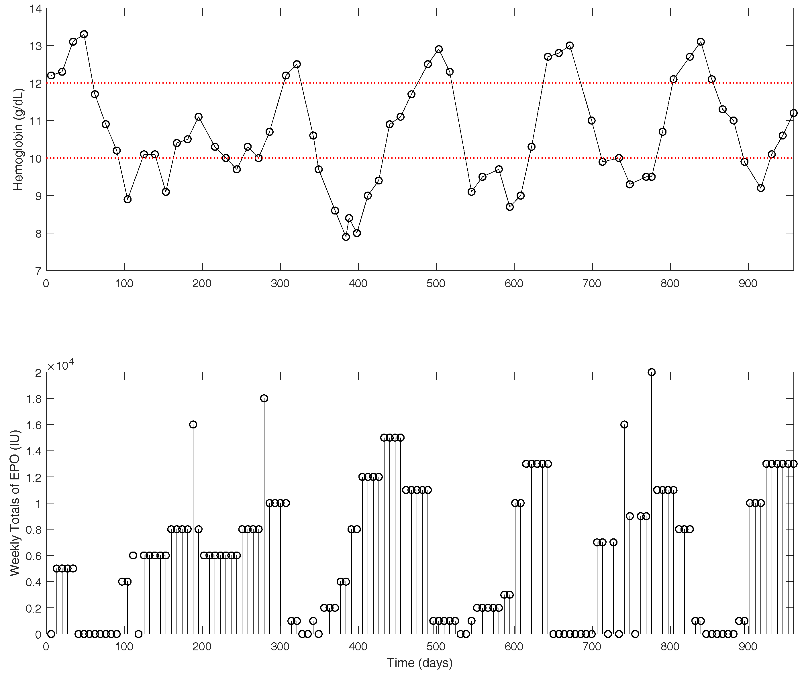
y represents the hemoglobin concentration in g/dL. Clinical data for an example patient are shown in
Figure 2. The hemoglobin measurements (top figure) are shown as the actual measurements recorded in approximately two-week intervals. The EPO doses (bottom figure) are presented as one-week dose totals. Typically, a dialysis patient with late stage renal disease will receive EPO medications 1–3 times per week, depending on dose size. With traditional dosing protocols, the oscillatory behavior observed in the hemoglobin is quite common [
24].
To estimate a patient’s hemoglobin response model, the cost function in Equation (
2) is used. It is the weighted least squares of the error between model predictions and actual hemoglobin values. The parameter
is used as a weighting value (
), to put a higher priority on newer measurements. The output
y represents the hemoglobin measurements.
where
and
represent the predicted and actual hemoglobin value, respectively. Equation (
3) represents the predicted hemoglobin using the historical data and the estimated model parameters (
) for a time horizon of 1 to
.
which can be compactly written as
where
is a vector of the optimized model parameters,
Y is the measured hemoglobin,
is the predicted hemoglobin, and
X is a matrix of the EPO dosage and measured hemoglobin concentration. Then, the objective function in Equation (
2) can be written as
where
,
, and
. The measurement weight in Equation (
2) is represented by the weighting matrix
R, which is a diagonal matrix of the weighting values
for each measurement.
Recursive modeling has been show to work well in cases where the model parameters are time varying, such as in Type 1 Diabetes Mellitus [
25]. Recursive modeling is the process of estimating a new patient model after each updated measurement. In this work, the patient’s model parameters are relearnt after each measurement, based on a moving window of estimation data. In the absence of validation data, constraints are used in the modeling formulation to ensure model stability, as well as to enforce that the model parameters follow patterns that are well described by many patients [
26]. The complete constrained ARX (C-ARX) model parameter estimation problem can be represented by Equation (5). Equation (5) assumes that the delay of the system is approximately two weeks. The peak time
parameter is shown here with a delay of two weeks (Equation (
5f)), and represents the largest contribution to the system of all the
parameters. The peak time
parameter can be shifted to the third or fourth week by reformulating constraints (Equation (5f,g)). Individual patient hemoglobin response times can vary. Some patients may begin to observe a substantial increase of hemoglobin in as little as two weeks, where some take much longer before a significant effect on the hemoglobin can be observed. The most appropriate way of dealing with the system’s unknown delay is to solve the same problem where the peak time
parameter is at the second, third and fourth delay, and then choose the solution with the lowest cost function. Equation (
5b) is used as a minimum and maximum range for the model estimates, as almost all the measurements should be within this range. Measurements that exist outside of this range may not be realistic, or may coincide with some abnormal event. Equation (
5c) is used to enforce model stability. Equation (
5d) is used to enforce a minimum response delay of two weeks. Equation (
5e) enforces that the model parameters are always positive, because the response of the system to the inputs is always positive. Equations (5f)–(5i) are defined through experience, and are used to enforce a particular parameter shape learned in [
26]. Finally, Equation (
5i) is used to ensure the model relies somewhat on the inputs to the system, and was determined through trial and error.
The above model is a constrained quadratic optimization problem and it is solved using the quadprog solver in MATLAB.
4. Conditional Value at Risk
The uncertainty considered in this work is in the form of process uncertainty on the output and can be represented by the variable
in Equation (
8).
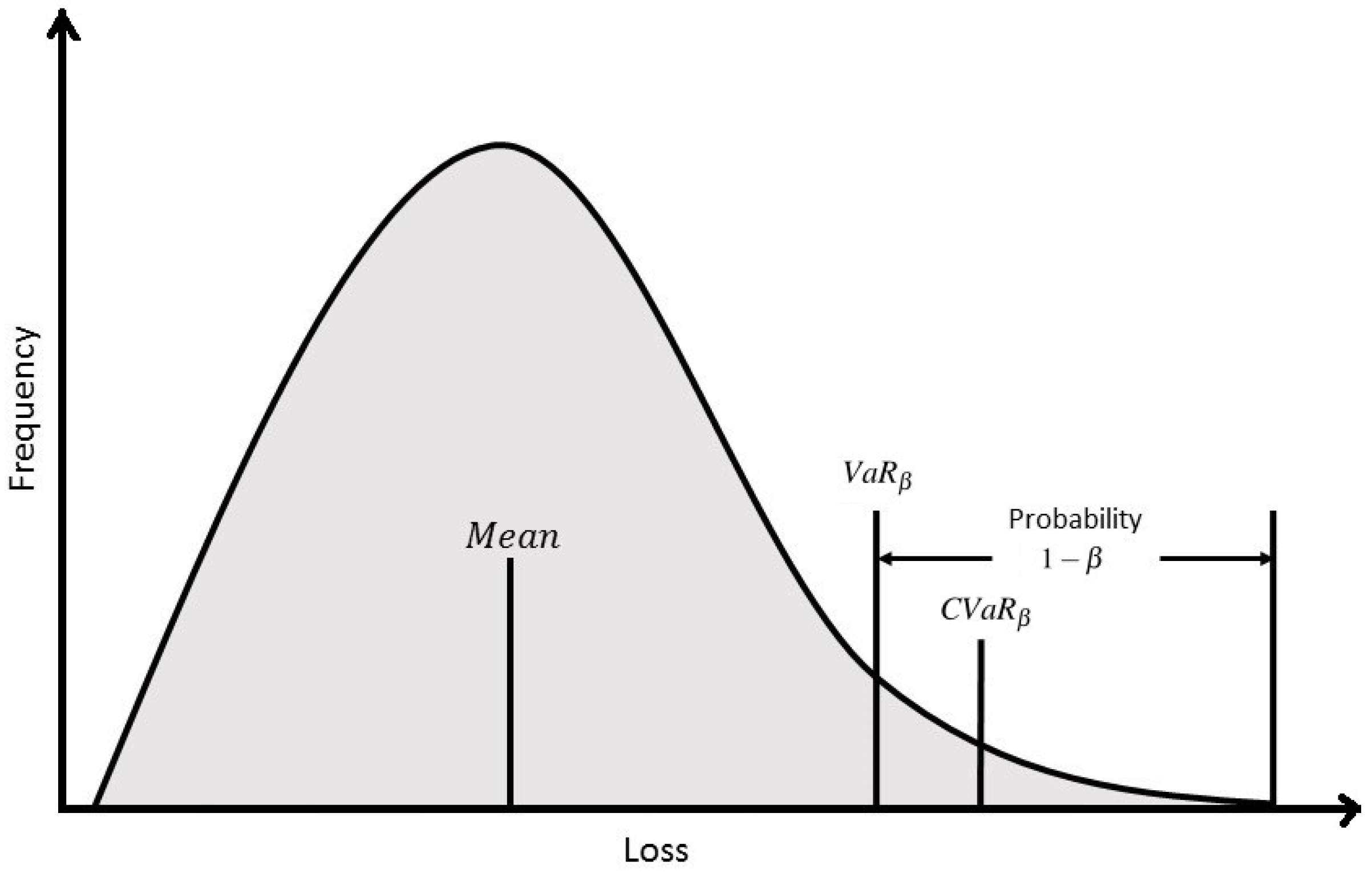
To address the uncertainty in the hemoglobin response to EPO dosage, this work studies two Conditional Value at Risk (CVaR) techniques for control under uncertainty. In general, Value at Risk (VaR) at confidence level
(
) is defined as the maximum loss value that is assigned to some desired probability,
. That is to mean that a loss less than or equal to
will occur
% of the time. What
fail to account for, is the losses that occur
of the time with a loss larger than
. CVaR at confidence level
(
) aims to minimize this loss and it is defined as the average of the loss exceeding
. For instance, a slightly higher
may be tolerated, if the average value of the
-tail distribution is lower. This would ensure that when a loss greater than
does occur, it will likely be smaller. A diagram is included in
Figure 4 to facilitate a better understanding of the value in which CVaR seeks to minimize.
Another major advantage of using CVaR constraints over other types of chance constraints, is that the uncertainty can follow any distribution. With a known distribution, different scenarios are generated for each sampling instant by sampling the random distribution. In this fashion, the controller optimization problem can take into account multiple scenarios, which help to approximate the different possibilities of measurement and process uncertainties, to ultimately provide a more robust solution.
Next, the CVaR technique is incorporated into the MPC formulation in two different ways. The first method handles chance constraints through CVaR approximation, whereas the second method directly optimizes CVaR in the cost function. Both controllers were tested in computer simulations against traditional zone-MPC and set-point tracking MPC to show the benefits that the two methods may provide.
5. Stochastic Control Using CVaR Constraints
The uncertainty is located within the output,
, in the form of a random variable
.
is assumed to follow a certain distribution. The controller is designed to take into account a process uncertainty from a known distribution. The optimization problem uses two chance constraints (Equations (9b) and (9c)) on the output of the system, one on the lower bound and the other one on the upper bound. Due to the conservative approximation of the chance constraint that the CVaR constraint results in, they will only be used for
, as shown below. If more constraints are used, the problem will become infeasible.
is not used because
, which means that, if the hemoglobin were to fall outside of the zone, the controller would only have a single input to try and move the hemoglobin into the zone to avoid infeasibility. The result would be a very aggressive control move in these scenarios that should be avoided. It should also be noted that the cost function is computed with Equation (
1), where
represents the predicted hemoglobin without uncertainty. Chance constraints are used in solving optimization problems under uncertainty. There exists uncertainty in the output prediction
, which is computed through Equation (
8). The meaning of the chance constraint is that utilizing some knowledge of the uncertainty in
, the constraint will be infeasible no more than
amount of the time.
is the probability of violation. The chance constrained set-point MPC formulation is proposed as following:
Due to the conservatism of the CVaR constraints, only a single point along the prediction horizon will utilize the constraints. Note that the
term is summed from 0 to
because
is always estimated as zero in the ARX model. The following derivations use a prediction horizon,
N, of eight weeks, and the ARX model introduced previously. Equation (
10) is used to demonstrate the derivation, which is the upper bound constraint [
17].
In the derivation below, the indicator function is used. This function holds a value of 1 if and a value of 0 if . For any positive parameter , we have . Defining an upper bounding function for the indicator function, the following inequality can be written.
Replacing u with , the following inequality can be written.
If
, the constraint is violated and the indicator function holds a value of 1, and vice versa.
is the upperbounding function for the indicator function and it is a conservative estimate of the probability of violation,
. From this, any solution that satisfies the inequality will also satisfy the constraint. The focus remains on the right side of this inequality. (u)
is defined as the maximum operator, which holds a maximum value between 0 and the input
u. Applying the upper bounding function
, a conservative approximation of the chance constraint is defined as
multiply by
moving
to the left hand side
To reduce conservatism, it is necessary to find the minimum that satisfies the inequality. That is, it is desired to find the smallest upperbound. This is a CVaR constraint, but it is difficult to calculate its value in its present form.
The expectation operator is removed with the introduction of sampling to approximate the CVaR constraint. M is the total number of scenarios. For instance, if there were a single random variable per scenario, and the prediction horizon was 1, it would be necessary to sample the random variables’ distribution M times. is the probability that a single scenario will occur, and is equal to . Note that changes to because the output is now an expected value with the uncertainty added in.
The expression inside of the max operator can be replaced by two separate constraints. Equation (18) replaces the max operator term with the variable
, and constraints are set on
to satisfy the original max operator’s functionality. The combination of all three constraints in Equation (18) can be used to provide a conservative estimate of the original chance constraint in Equation (10) through the use of sampling [
18]. These constraints are solved using many different scenarios of the random variable distribution, leading to it being part of a class of controllers called Scenario-Based MPC.
Similarly, for the lower bound constraints, we have the following approximation
Finally, notice that the cost function in Equation (9) contains absolute terms. This equation can be manipulated to remove the absolute sign and the resulting linear program with all the constraints is outlined in Equation (20).
where
is the Hb prediction from the ARX model without process uncertainty term.
Summarizing the above derivations, the complete deterministic approximation to the chance constrained set-point MPC formulation is given as follows:
There are constraints and the optimization vector consists of variables. The controller optimization problem involves the use of M scenarios, where M typically holds a value larger than 100 and is selected by the user. A single scenario is simply the trajectory of the hemoglobin response while including uncertainty values drawn randomly from the known uncertainty distribution. It should quickly become apparent that scenario-based constraints such as these lead to a very large number of constraints, with constraints related to the CVaR constraints alone. With this in mind, the cost function used in this design is a linear program and MATLAB’s linprog function was used along with its dual-simplex optimization algorithm. This controller is referred to as CVaR below.
6. Stochastic Control Using a CVaR Cost Function
The second method discussed in this work optimizes the control inputs using conditional value at risk directly within the cost function. In contrast to the first method, the solution to this optimization problem is always feasible. The controller derivation follows the work of [
17,
19] closely, but with the exception that the algorithm is modified to use a zone-MPC formulation. The optimal solution can be thought of as the solution that minimizes the average loss that occurs in the
-tail distribution of the probability density function (pdf) of the loss function. The controller formulation in Equation (22) uses the distribution of the random variable,
, to generate several different plausible scenarios of process uncertainty.
where the cost function is given as
The loss function is associated with decision variables and auxiliary variables and random variables . Note that Q is the tuning parameter in this equation and zone control is facilitated through the use of the variable . The conditional expectation of loss in the bad tail leads to the idea of Conditional Value at Risk. is defined as the conditional expectation of the loss above
Rockafellar and Uryasev [
17] showed that the
can be determined as follows
denotes the max of
.
ℓ is an auxiliary variable (can be viewed as
) to be optimized. The integral can be approximated by sampling of the random variable:
with probability
The absolute terms from Equation (
23) can be linearized by introducing variables
and
. Note that
represents the expected output for the scenario.
Then, by combining Equations (
26) and (27), the CVaR cost can be written as
This is equivalent to
The variable is introduced to allow the calculation of the max operator. The final form of the stochastic MPC problem is a linear program outlined in Equation (30) that minimizes the , where represent the sampling instant, scenario number and sampling instant along the prediction horizon, respectively.
The above Equation results in constraints and an optimization vector length of . This controller is referred to as CVaR below.
7. Computer Simulation Results
The following section outlines the experimental design and the simulation results comparing the CVaR methods to set-point tracking MPC and zone-MPC for both Gaussian and uniform distributions, for both an ARX model based patient simulator and a pharmacokinetics and pharmacodynamics (PK/PD) model based simulator.
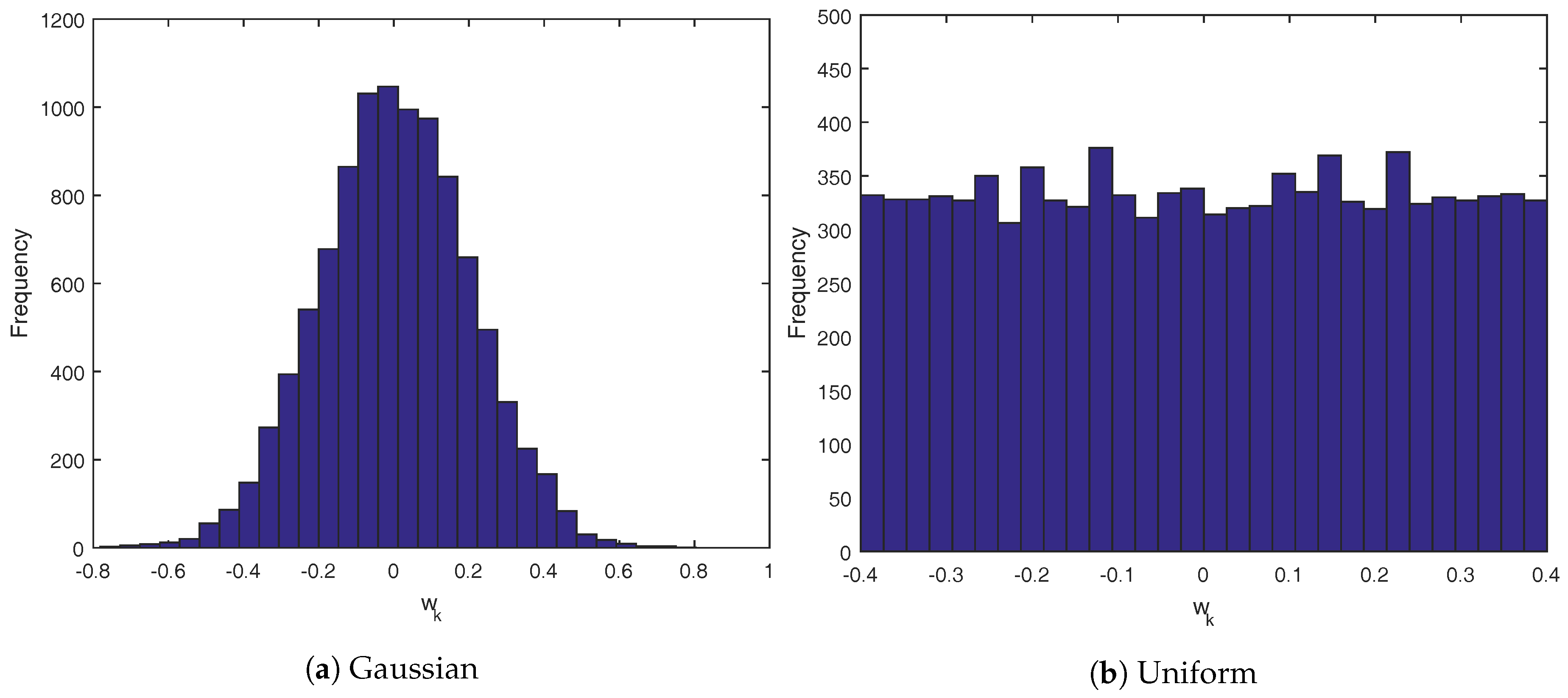
Both simulator cases use the same Gaussian and uniform distributions for the random variable
. The histograms are outlined in
Figure 5.
Figure 5a follows a Gaussian distribution of
, while
Figure 5b is a uniform distribution of
. In all cases, the controllers that use the CVaR technique were given the exact distribution of
to calculate the scenarios for each controller iteration. For these simulations, each scenario would draw random variables for each sampling time in the future that is used in the controller design. For instance, in the first CVaR controller, the uncertainty is only needed up to
for each sampling instant, meaning there are only three values drawn from the uncertainty distribution for each scenario. In the second CVaR controller, it draws the full eight weeks of values for each scenario.
The performance of the controllers are measured based on four metrics. The state performance metrics are the integrated output error (IOE) outside of the control zone, and the percent of points in the zone (PIZ). The input metrics are average weekly EPO dose (EPO/week) and the average weekly change in dose (avg ). The four performance metrics can be calculated using Equation (31).
7.1. Test under An ARX Model Based Simulator
The ARX model based simulations were performed without time-varying parameters and recursive modeling. These simulations represent a nominal case, where the patient model does not change. A single constrained-ARX model was used. A simulation time of 2000 weeks was used, to obtain better statistical power of the results. A sampling time of one week was used. The controller tuning parameters are shown in
Table 1. The tuning parameters were defined empirically, to limit the Average Change in EPO parameters to be low. In practice, EPO is often administered in 1000 IU increments, so the controllers were tuned to have the average weekly change less than this value.
The results for the Gaussian distribution simulation are outlined in
Table 2. The CVaR formulations offer significant improvements over traditional zone-MPC, but their performance is only marginally better than set-point tracking MPC. The time to solve is included in the table. Due to the large number of added variables introduced for sampling in the CVaR controllers, the time per iteration also increases.
The results for the uniform distribution are outlined in
Table 3 and
Table 4. CVaR
has a large increase in the state performance over set-point tracking MPC, but it comes at the cost of an aggressive control action. The overall statistics show the controller to be more aggressive, but in fact it is actually quite stable with regards to its control input action.
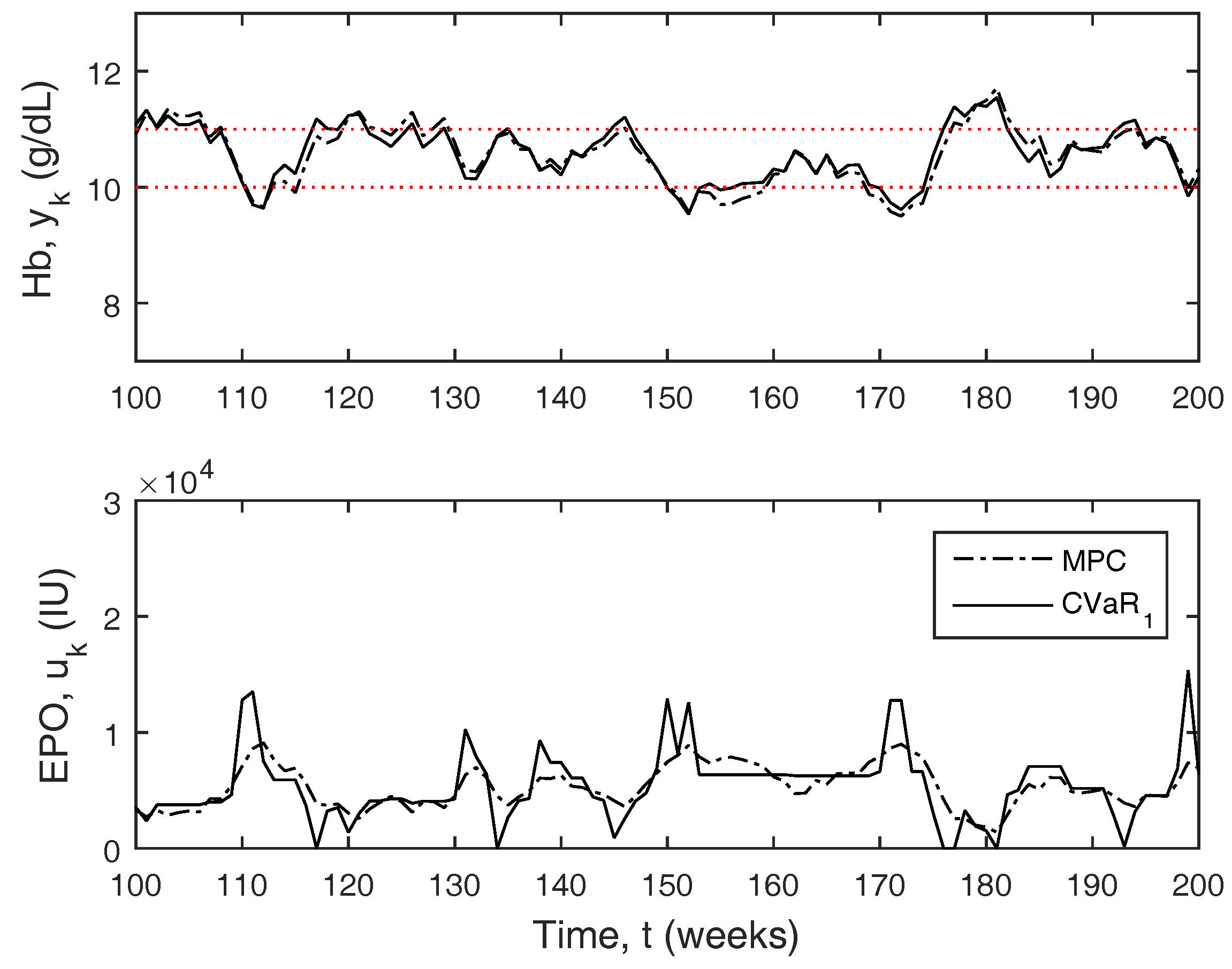
Figure 6 depicts a small window of the full 2000 week simulation results comparing MPC to CVaR
. CVaR
behaves similar to zone-MPC, but the controller will be extra aggressive outside of the zone boundary as the hemoglobin approaches the constraint boundaries. The overall aggressiveness of the controller is much larger due to these larger moves, even though the doses are typically more stable.
Figure 7 compares CVaR
to zone-MPC. As compared to zone-MPC, the response is much better, as the CVaR is able to pre-emptively change the dose in anticipation of the hemoglobin leaving the zone, whereas zone-MPC only reacts to the hemoglobin leaving the zone, causing it to traverse beyond the zone boundaries more often.
7.2. Test under PK/PD Model Based Simulator
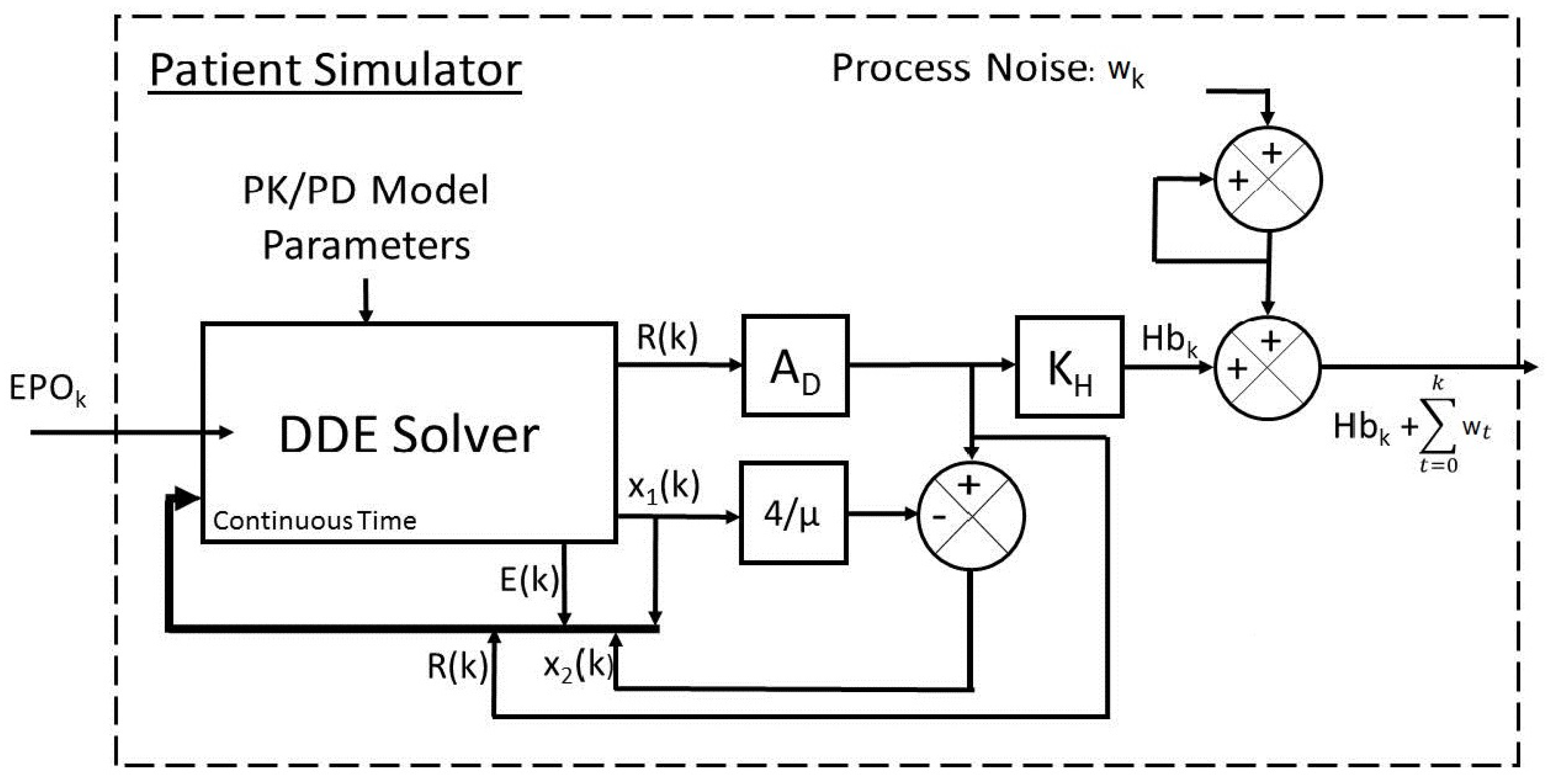
For this test, the patient simulator shown in
Figure 8 was used which was designed in detail in [
23]. The patient simulator represents a more realistic scenario to test the controllers with. The patient simulator uses a system of nonlinear delayed differential equations (DDE) based on pharmacokinetics and pharmacodynamics to model hemoglobin response.
The DDE model was proposed by Chait et al. [
11]. Pharmacokinetics is the study of the movement of drugs within the body while pharmacodynamics is related to the mechanisms by which the drugs affect the body. The PK/PD model is described below.
In Equation (32), states
and
represent the pool of exogenous erythropoietin and the population of red blood cells (RBC) within the body, respectively. States
and
are internal states that aid in calculating
.
is the endogenous erythropoietin naturally produced by the body.
is the average amount of hemoglobin per RBC (also known as the mean corpuscular hemoglobin, MCH). The value used here is fixed at 29.5 pg/cell, which is within the reference range of 27–33 pg/cell [
11]. The hemoglobin value is directly proportionate to the RBC population; the hemoglobin value can be attained by multiplying the RBC population estimate by the MCH value. The function
is a train of impulses, representing the EPO injections. The model has an initial condition as represented in Equation (33) and requires two measurements of hemoglobin (
) and the time in between those measurements (
) to estimate. The prior history of the exogenous EPO is unknown, and assumed to be zero for all
.
Table 5 contains parameters that are estimated for an individual patient using clinical data and nonlinear least-squares regression. The
dde23 and
lsqnonlin functions in MATLAB were used for DDE solution and parameter estimation, respectively.
The DDE model is solved in continuous time and sampled every two weeks. The output of the DDE model is the red blood cell population (), which is multiplied by the mean corpuscular hemoglobin () to get the hemoglobin measurement. The hemoglobin measurement is then added to an integrating process uncertainty (). It is important to note the difference between the ARX model simulator and PK/PD model simulator in regards to the way is used. In the ARX simulator case, is filtered with the patient model. In the PK/PD simulator case, the disturbance is integrating. The magnitudes are drawn from the same distributions in both cases.
The simulator also includes the possibility of acute step and ramp disturbances to simulate infections and blood losses frequently observed in actual patient data. Acute disturbances are facilitated through the use of the variable
, which holds a value of one unless a disturbance has occurred. If an acute disturbance occurs, it will hold a value less than 1, and the existing pool of red blood cells in the patient simulator model is multiplied by the fractional value to reduce it. A step disturbance is then modeled by an impulse in
, while an infection is modeled by a step function in
. Plant–model mismatch exists as the controller model is linear. The patient simulator was shown to mimic the real life hemoglobin system dynamics of patients well [
23]. The total simulation time was 500 weeks. Recursive modeling is necessary to capture the time-varying nature of the system model. Although the patient model does not change significantly from sampling interval to sampling interval, the patient model is still re-estimated to provide continuity between the models at each sampling interval. A hemoglobin sampling time of two weeks is used, and two weekly dose total inputs solved by the controller are used during each sampling interval. The recursive modeling method applies a data re-sampling algorithm to get one week measurements (through linear interpolation), and weekly dose totals. The one-week re-sampled hemoglobin history is also smoothed, using a five-point moving average filter, before modeling occurs. The weighting parameter
is set to 0.965. The tuning parameters for each of the controllers are outlined in
Table 6. The tuning parameters were again defined empirically. For these simulations, the Avg
was tuned to be approximately equal in most cases to better compare the controller results to one other.
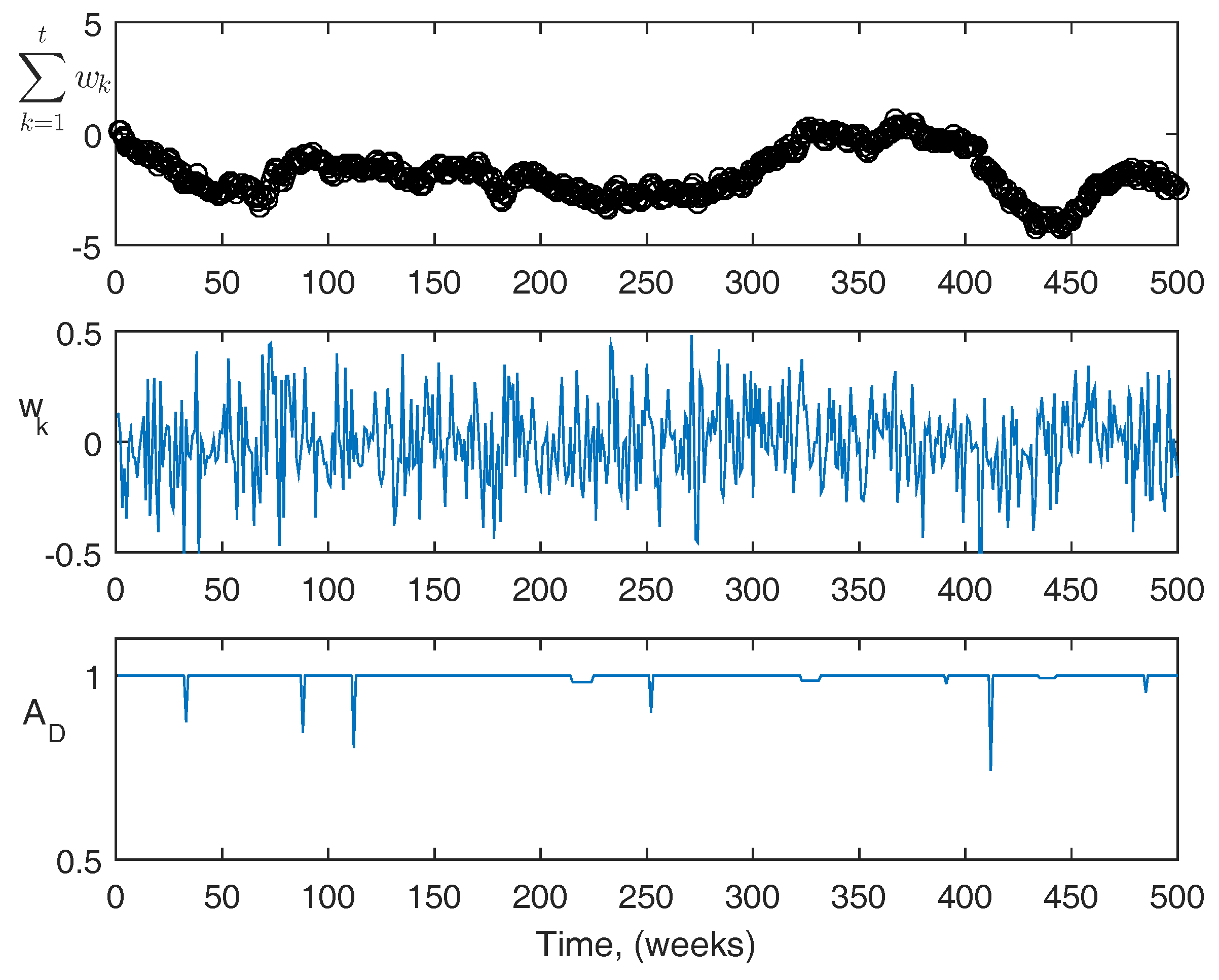
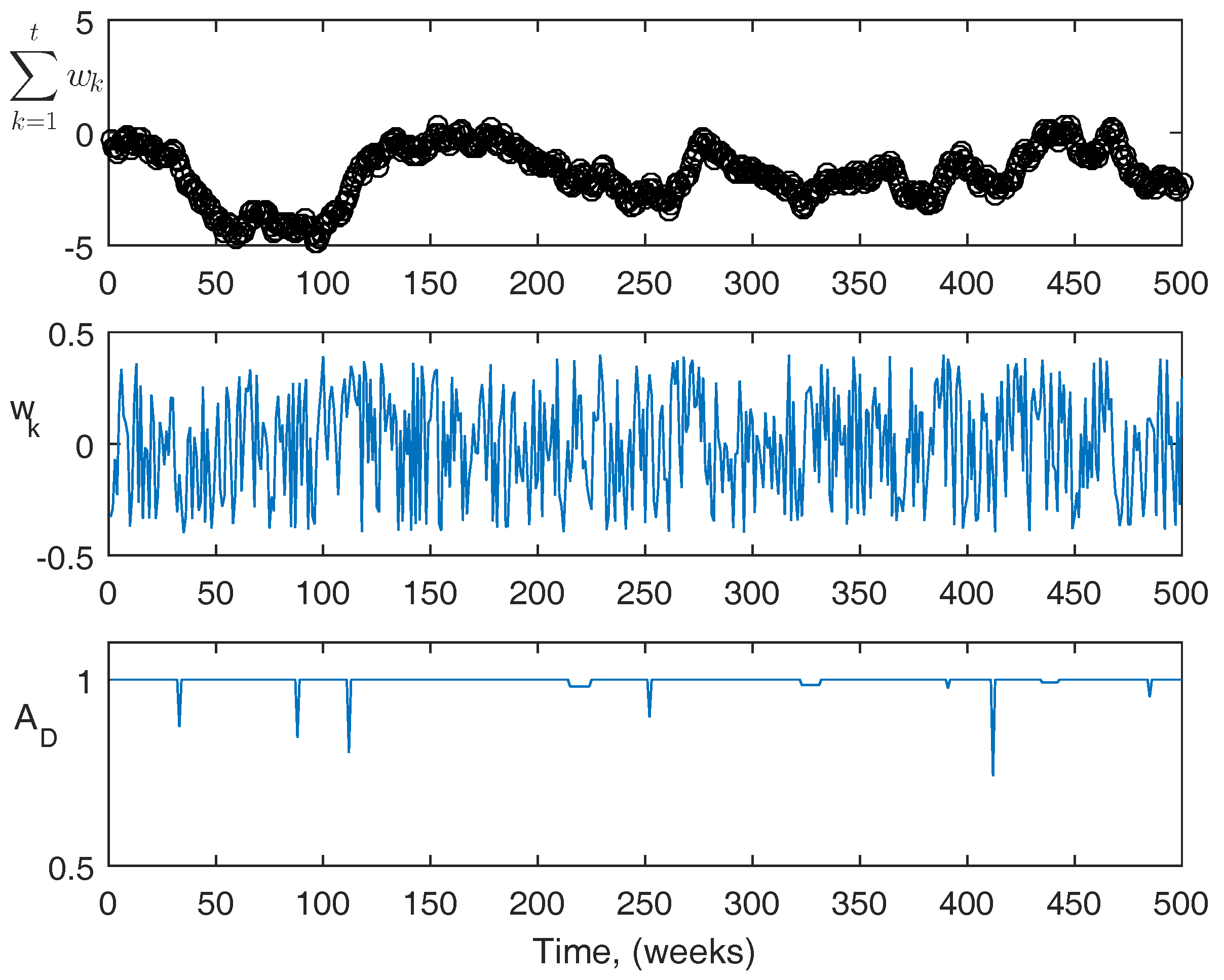
For reference, more information about the actual disturbances is shown in
Figure 9 and
Figure 10. The top figures are the summation of the disturbance over the course of the simulation. The center figures are the magnitude of the disturbance at each point. The third figures are the acute disturbances that occur during the simulation, which are the same in both cases. In the simulation, the acute disturbances include seven blood loss events, and three infection events in both cases. The PK/PD parameters used in the simulator are as follows:
,
,
,
,
,
,
, and
.
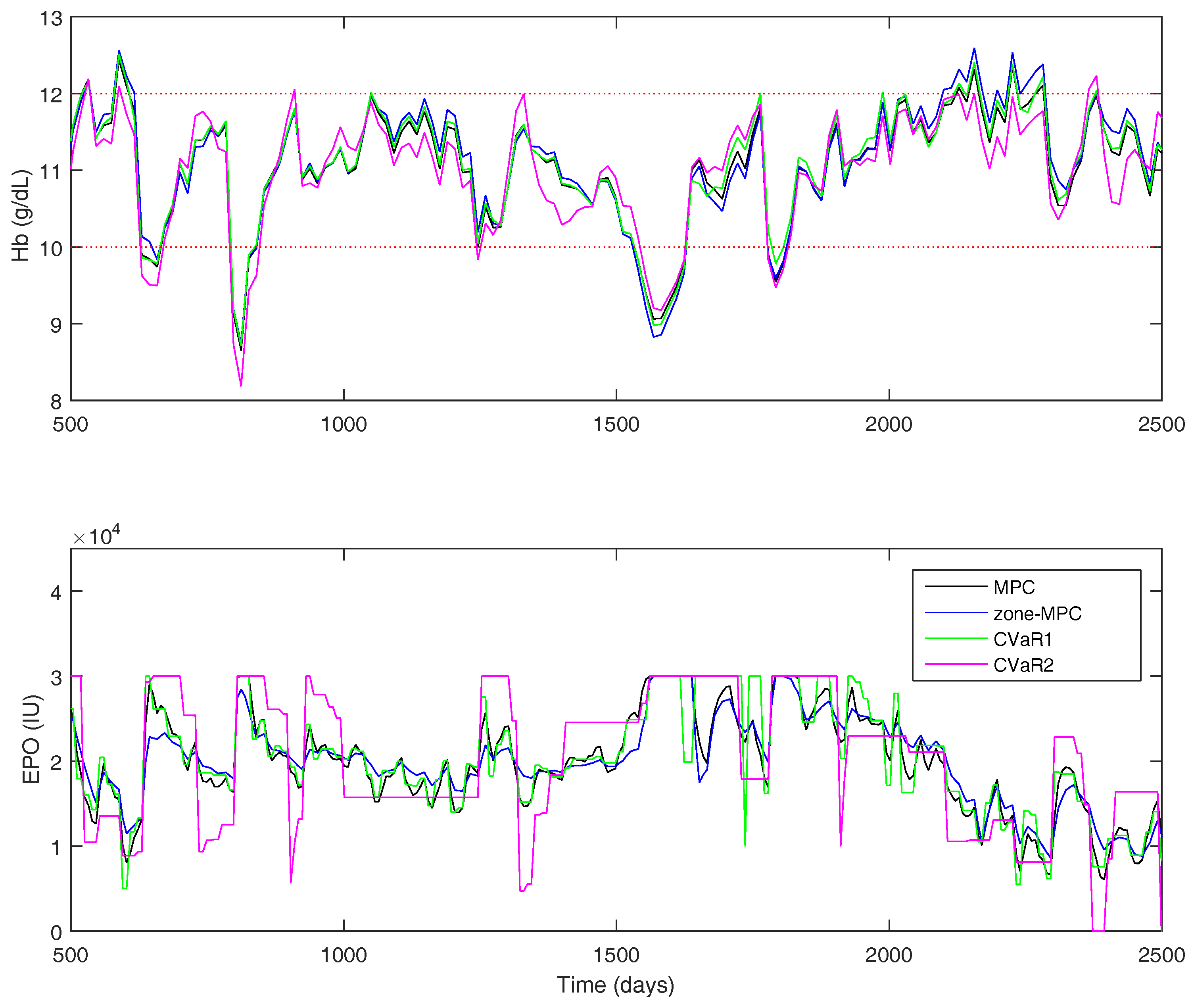
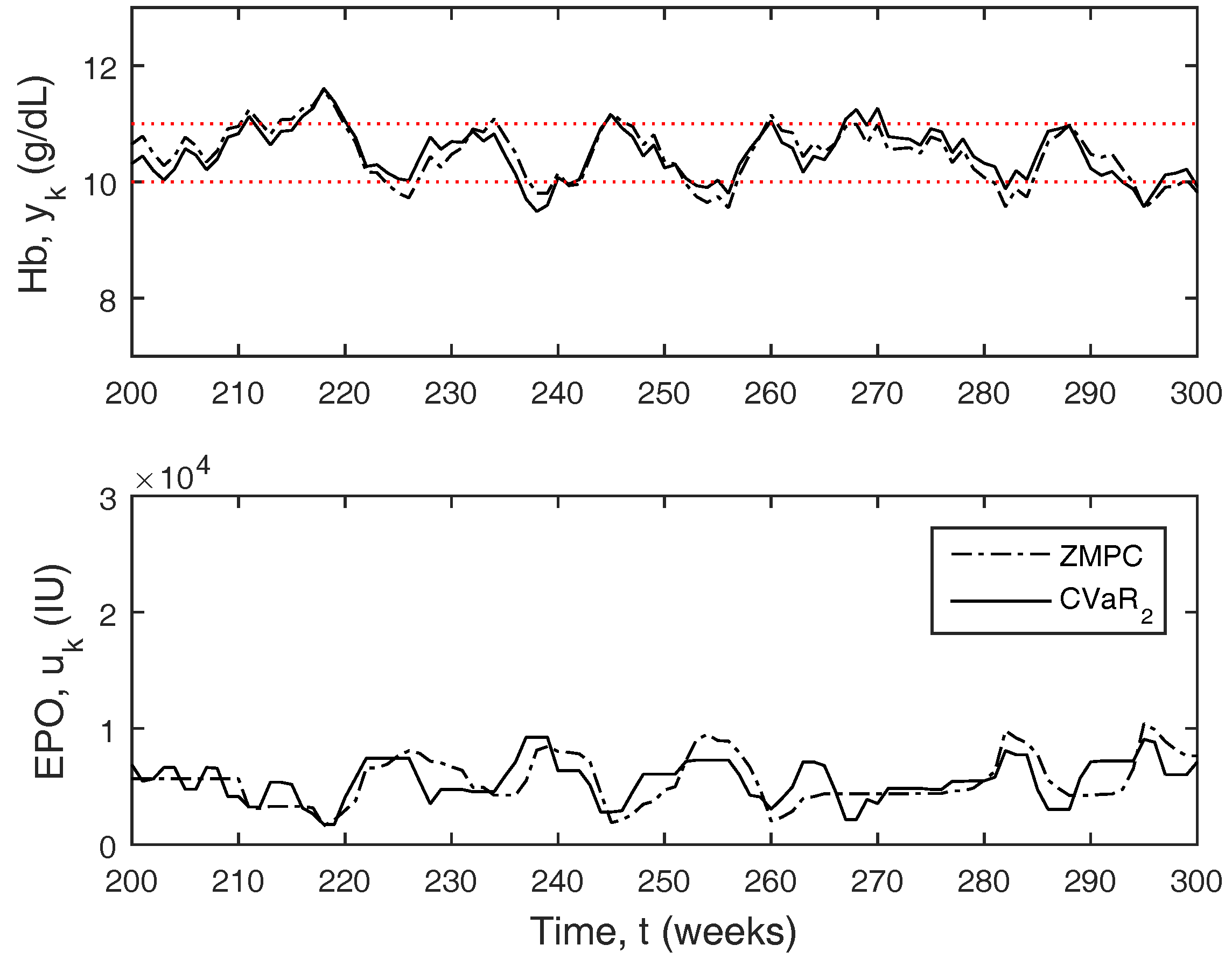
The results for the Gaussian uncertainty case are presented in
Table 7. The four controllers’ performance statistics are shown in
Figure 11 for a portion of the full 500-week simulation. The tuning parameters were chosen to try and keep the controller average
approximately equal, so it is easier to compare the state performance between the controllers. However, the zone-MPC controller is unable to reach the same level of aggressiveness as the other three without becoming relatively unstable. Using the CVaR constraints improves the performance drastically over zone-MPC, and offers modest improvements over traditional MPC. Using CVaR in the cost function, offers similar state performance to that of set-point tracking MPC, with the same average control action. Using CVaR in the cost function allows the medication dosing to remain stable when the hemoglobin is within the zone. As it nears the borders, the controller will typically make large moves in the medication dose. Overall, the medication dose remains very stable, even though the average
does not portray this feature in the statistics.
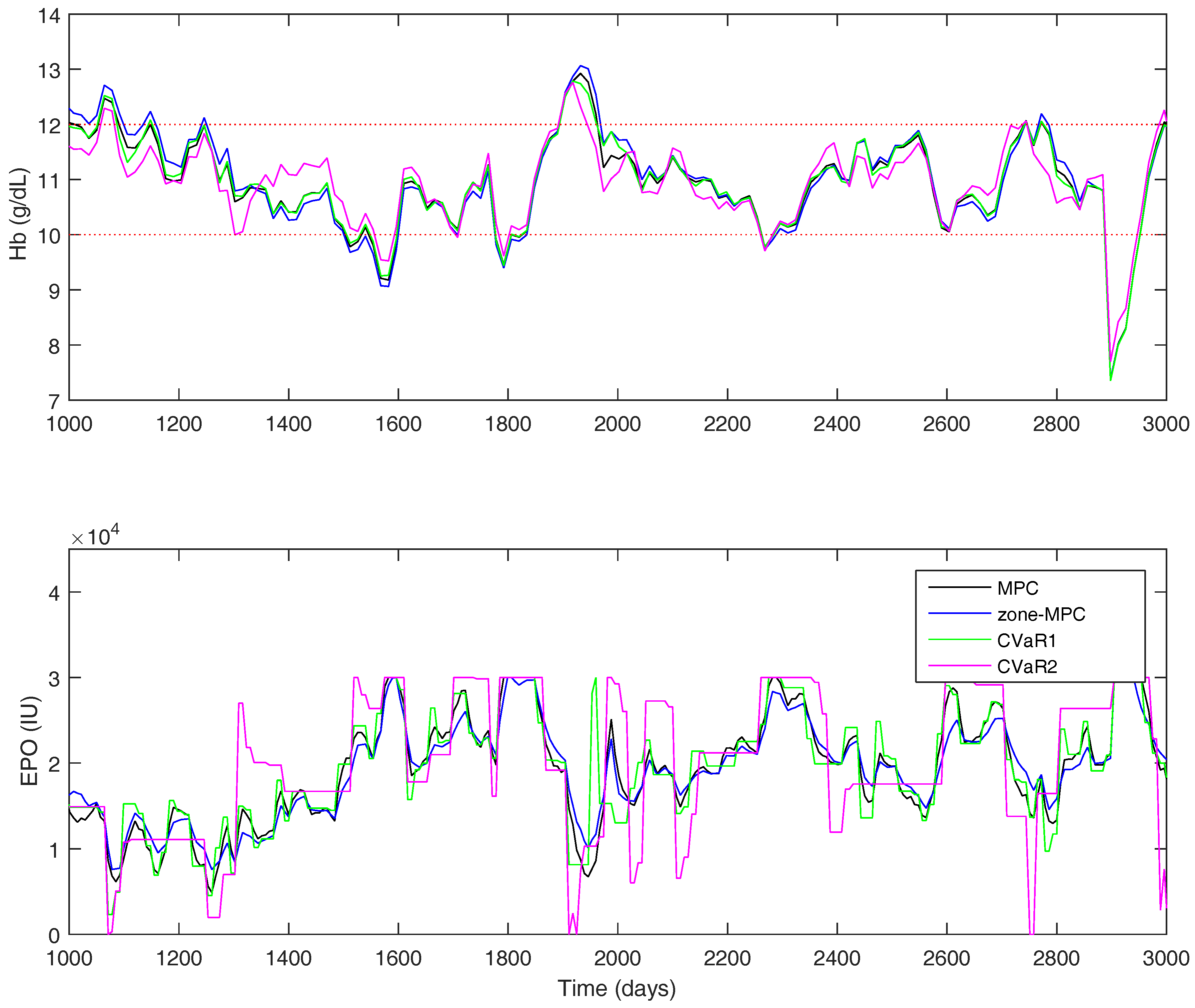
For the uniform distribution case, the overall results are shown in
Table 8. A short window of the overall simulation can be seen in
Figure 12. The CVaR constraints allow the controller to significantly improve the PIZ metric over the other controllers, while remaining with a similar average controller aggressiveness. Using CVaR in the cost function has an average change in dose similar to MPC and
, but, looking at
Figure 12, it is again easy to see that the controller rarely changes the medication dose, but, when it does so, it is typically a significant move.


