Receding Horizon Optimization of Wind Farm Active Power Distribution with Power Tracking Error and Transmission Loss

Abstract

In this paper, a receding-horizon optimization strategy is introduced to optimize the wind farm active power distribution with power tracking error and transmission loss. Based on the wind farm transmission connections, a wind farm can be divided into clusters, in which the wind turbine generator systems connected to one booster station can be taken as one cluster, and different clusters connected from booster stations to the farm-level main transformer output the electric power to the grid. Thus, in the proposed strategy, the power tracking characteristic of the wind turbine generator system is modeled as a first-order system to quantify the power tracking error during the power tracking dynamic process, where the power transmission losses from wind turbine generator systems to booster stations are also modeled and considered in the optimization. The proposed strategy is applied to distribute the active power set-point within a cluster while the clusters’ set-point still follows the conventional strategy of the wind farm. Simulation results show significant improvement for both optimization targets of the proposed strategy.

1. Introduction

With the development of modern electric energy, wind energy has been developed rapidly due to the environmentally friendly features. From an energy conversion perspective, the wind turbine generator system (WTGS) is the device that converts wind energy into electrical energy, which takes the active power set-point as input and outputs the electric power to the grid. Controllers within the WTGS are working in coordination to guarantee the WTGS power output tracks the power demand [1]. Over the past few years, many achievements have been introduced in wind turbine control to improve the wind turbine load conditions and stabilize the power output. Usually the wind turbine is mainly controlled with different targets by region.When the wind speed is between the cut-in wind speed and the rated wind speed, the maximum power point track (MPPT) strategy will be adopted to control the generator torque which guarantees that the WTGS will follow the optimal tip speed ratio and optimal wind-power utilization coefficient [2]. When the wind speed is above the rated speed, a power limitation strategy will be used to limit the power at the rated condition [3]. When the power demand is lower than the WTGS capacity, the power limitation strategy will also be used to limit the generator power output to meet the power demand. From another perspective, when the wind turbine nonlinear dynamic characteristic and the turbine stochastic behavior caused by wind speed randomness are concerned, research has been done to optimize the wind turbine control [4,5].

In the industrial field, WTGSs are organized and controlled under a wind farm. A wind farm usually contains several WTGSs and serves as a control and transmission center between WTGSs and the electric power grid. The wind farm will calculate the predicted farm available power based on the wind speed predictions and upload the predicted result to the power grid dispatch center. It will then take the wind farm power demand set-point from the dispatch center and control the power set-point for each inner WTGSs to make sure the wind farm power output follows the power demand. Typical wind farm power strategies can be referred to from [6,7]. Since the wind farm power output is usually less than the available power, WTGSs in the wind farm may limit the power output to less than the available power and the reserved part can be used for further improvement. One proposed wind farm distributed model is where predictive control with a clustering-based piece-wise affine wind turbine model, where the complete wind turbine model is used and the wind farm is set to track the active power output as the conventional strategy while reducing the wind turbine loads, [8,9]. Another farm-level load-reduction strategy is introduced in [10,11], of which the power tracking error and load conditions are all considered in the cost function and solved by a centralized model predictive controller. In [12], a distributed model predictive control strategy is also applied in wind farm active power control to optimize the wind farm power output. Both dual decomposition based on fast gradient updates (DDFG) and alternating direction method of multipliers (ADMM) methods are introduced to solve the optimization problem distributively or in parallel in favor of fast solving for wind farm active power control. When the wind farm is connected into the power grid, voltage will be an important parameter that will need to be considered. In [13] proposes a VSC-HVDC (Voltage Source Converter based High Voltage Direct Current Transmission) connected wind farm active control when the voltage variation is taken into consideration to improve the wind farm voltage control performance. Since the WTGSs in the wind farm are growing in numbers, the optimization problem from the wind farm level will also increase in orders and solving time. Some corresponding decentralized strategies are also investigated in wind farm power and voltage control process to reach an acceptable control effect. Related researches can be referred to [14,15]. With the increasing proportion of the wind power in the power system, wind power gradually begins to assume the task of peak load and frequency regulation of the power system as an important part of the power supply side [16]. The work in [17] reviews some wind farm active power control methods where the wind farm can be regarded as a frequency modulation unit to balance the power grid electric supply and demand, and further support the grid frequency under emergency conditions.

In addition to the wind power related research, there have been many experts and scholars who analyze other aspects to improve the environmental friendliness of current energy systems. Renewable energies could be connected together to the electric power system which can cause problems in power system integration and control. The work in [18] proposes the modeling and control design for a novel model of smart grid-connected PV/WT (Photovoltaic Module/Wind Turbine) hybrid systems. All of the photo-voltaic array, wind turbine, asynchronous (induction) generator, controller and converters are integrated in the designed power system. Considering that the optimization process usually contains more than one optimization target, several multi-objective optimization strategies have been adopted in energy systems and industrial processes. A novel combined cooling, heating and power (CCHP) based compressed air energy storage system is proposed in [19], in which the evolutionary multi-objective algorithm is used to optimize the overall exergy efficiency and the total specific cost of product of the novel CCHP system. In [20,21] they propose multi-objective energy benchmarks based on the energy consumption forecast and integrated assessment. The method for developing the dynamic energy benchmark for mass production in machining systems is also introduced. These works provide advanced strategies for energy systems from different perspectives for different application objects, which are also useful for the work in this paper.

Usually, the wind farm power set-point is less than or equal to the wind farm prediction available power. When the power set-point is equal to the available power, wind turbines in the wind farm output all the available power to track the power demand. There would be no power distribution process under such a condition and all units are free to generate electricity. In the other circumstance, a power limitation strategy is needed. The wind farm control center will dispatch the power set-point to all units according to the available power of each unit to make sure the power output is following power set-point. Under such a circumstance, the unit power output will be less than the available power. The gap between the power set-point and available power could be adopted for further improvement. Although the previous strategies are useful and efficient, there still exist several potential parts which can be further improved in details. Firstly, with the increased number of WTGSs in a wind farm, wind farm capacity is growing and the power loss caused by power transmission is also growing significantly. WTGSs are usually connected to booster stations before the farm level main transformer, and the transmission line between WTGSs to the booster stations is usually with lower or medium voltage level, which plays the most significant role in power transmission loss. Since the transmission line between different units to booster stations are different, the transmission loss characteristics between units are usually different and should be taken into consideration during wind farm active power distribution. Secondly, the wind farm power output usually fluctuates around the wind farm power set-point due to the WTGS power tracking process, the power tracking error should be reduced or even eliminated through improving the wind farm control algorithm.

As the main contribution of this paper, a wind farm active power distribution strategy is proposed to improve the wind farm power output and power loss caused by transmissions. WTGSs are investigated with the power tracking characteristics and power transmission losses. Firstly, the WTGS power tracking process is modeled as a first-order inertial link. Furthermore, the control horizon recedes with time and the power tracking error caused by WTGS dynamic characteristic will be modeled in the optimization cost function, which would be minimized during the control horizon. Besides, the wind farm transmission loss is also served as another part in the cost function. In Section 2, a typical wind farm topology and the power transmission loss are firstly introduced. In Section 3, the WTGS power tracking dynamic characteristic is modeled as a first-order inertial link. The proposed wind farm active power receding horizon control strategy is introduced in Section 4, where the corresponding predictive model, cost function and constraints are explained in details. To verify the effectiveness of the proposed strategy, a wind farm with 20 units is defined and simulated in Section 5. Both the conventional strategy and the proposed strategy are adopted and compared to show the difference. The proposed strategy is shown to be a feasible and effective strategy that improves the wind farm in both power tracking error and transmission loss. Section 6 concludes this paper.

2. Wind Farm Topology and Power Transmission Loss

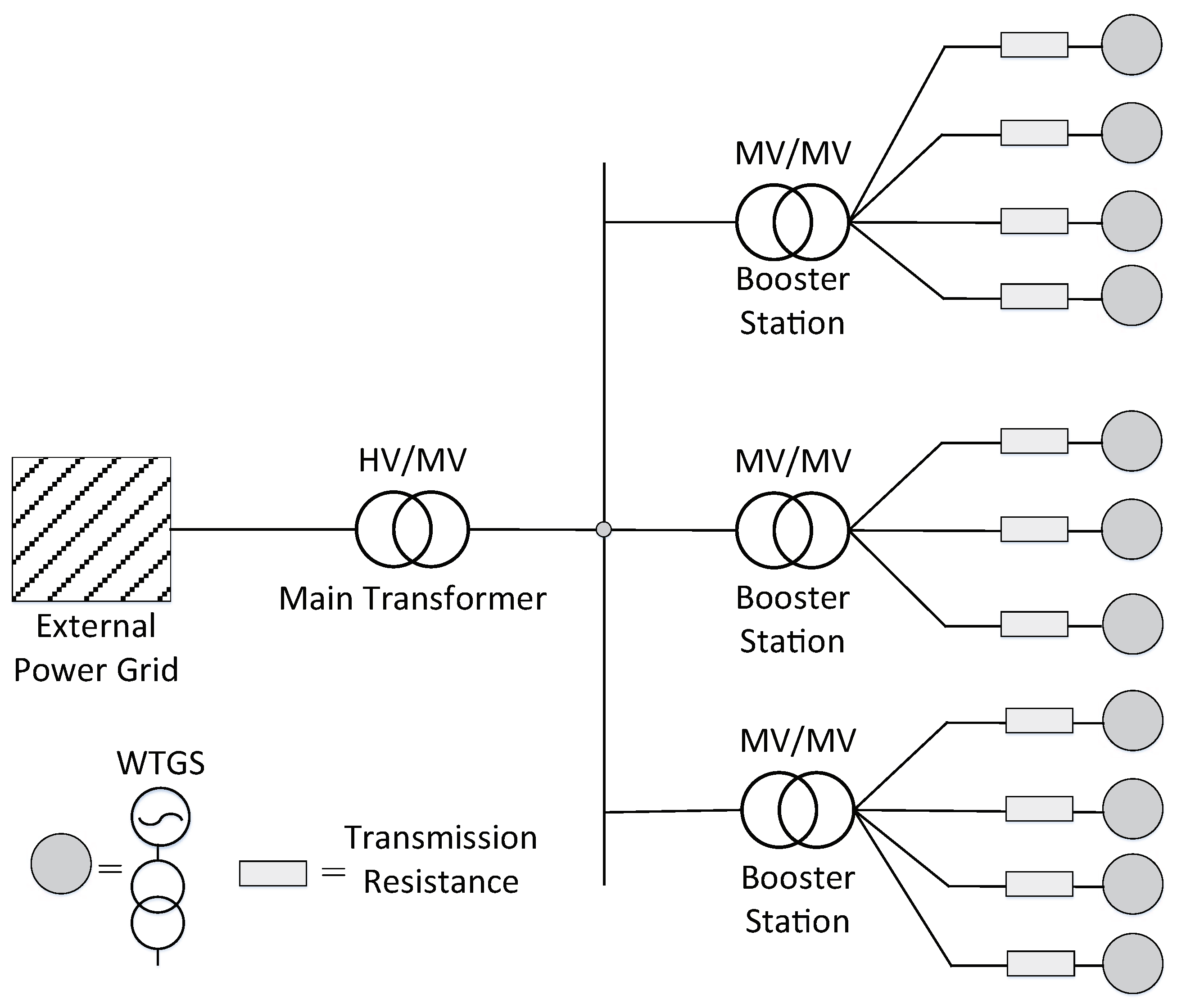
As is known, a number of wind turbines work together in a wind farm, which are usually controlled uniformly to make sure the wind farm power output follows the power demand set-point from the power grid. Considering the electric power output from WTGSs is usually in a middle level voltage, a double layer booster structure usually exists in the wind farm to increase the electric voltage before connected to the power grid, the WTGSs in the wind farm can be divided into clusters by the booster station connections. Several WTGSs within an area are connected under one booster station, the boost station will increase the voltage (from 33 kV to 110 kV) and different booster stations are connected to the wind farm main transformer, through which the voltage will be further improved (from 110 kV to 330 kV) and then output to the external electric power grid. A typical wind farm topology can be shown as Figure 1. In this figure, MV and HV are rating on the voltage level, where MV is medium voltage, and HV is high voltage. The voltage rating might be different under different scenarios. In usual, HV stands for the voltage higher than 110 kv, and MV stands for a voltage level between 3 kV to 110 kV. LV may also be used as for low voltage which indicates a voltage level under 3 kV. It should be noted that, the voltage level at booster stations or transformers and the wind farm topology may be different since the wind farm may follow different standard files. The listed numbers and topology is only one typical condition, which is considered in this study.

The power transmission loss is defined as the power loss due to the transmission line between WTGSs and the booster station, i.e., the resistance on the transmission line causes a drop in power at the front and rear of the transmission. Limited by the voltage, the power loss between WTGSs and booster stations is the main part in the wind farm power transmission loss. After the booster device, the increase in voltage will decrease the current and reduce power loss due to resistance electro-thermal effect. Since the transmission line between WTGSs and booster stations are with the same material and thickness, the increase in distance will proportionally increase the transmission resistance. On the other hand, the transmission loss is proportional to the squared transfer current, and WTGSs usually output electric power as a constant voltage source:

$$M\propto I^2={\left(\frac{P}{U}\right)}^2,$$

(1)

in which I is the transmission current on the transmission line, P is the transmission power which is also the active power output of the considered unit, and U is the transmission voltage. Thus the transmission loss can be simplified and expressed in the following form:

$$M=K\times P^2\times D,$$

(2)

in which M is the power transmission loss due to the resistance electro-thermal effect, D is the distance between WTGSs and booster stations, P is the WTGS output power and K is a constant number to assist in calculation. Set $K=1$ and $M=P^2\times D$ can be used as a simplified form to calculate transmission loss, which serves as a cost function during the active power distribution.

3. WTGS Power Tracking Dynamic Characteristic Modeling

The WTGS is essentially a nonlinear model with multiple variables and controllers to capture the wind energy and transform it into electric power. The wind-turbine cluster is defined as a cluster of WTGSs which can be controlled and scheduled uniformly. As shown in Figure 1, several WTGSs are connected under one booster station and can be selected as a cluster and controlled uniformly. In this section, the WTGS power tracking dynamic characteristic will be analyzed and modeled in favor of the wind-turbine cluster active power control strategy.

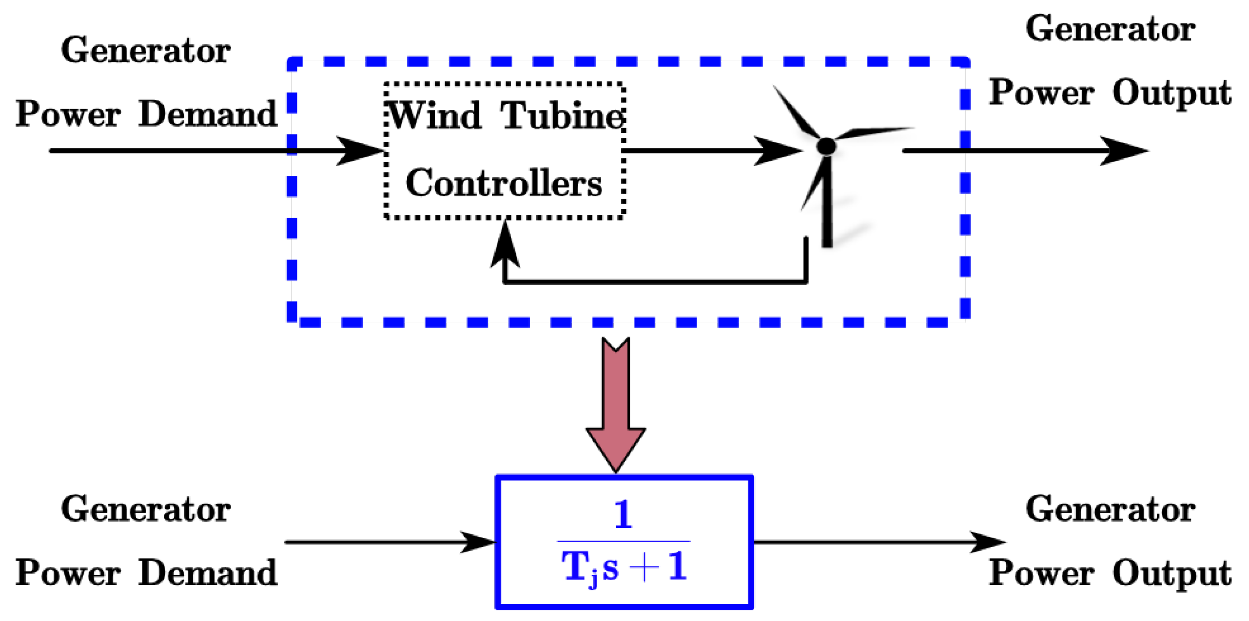
From the control design perspective, the blade pitch controller, the generator torque controller and the yaw controller are working in coordination to ensure the WTGS is functional. But from the energy transfer perspective, a WTGS usually receives active power orders from the active power controller in the wind-farm level, then adjusts the inside controllers to make sure that the generator power output catches up with the active power demand. In such a situation, the inner controllers can be regarded as WTGS inherent modules. The dynamic characteristic of power tracking for a WTGS can be reduced to a first-order inertial link from the active power demand to the generator power output, for which the input is the WTGS active power set-point from the wind farm and the output is the generator power output. The WTGS power tracking dynamic characteristic can be expressed as follows:

$$P_i^{out}=\frac{1}{T_{i}s+1}{P}_i^{set},$$

(3)

where i represents the i-th wind turbine, $P_i^{set}$ is the active power set-point for the i-th WTGS, and $P_i^{out}$ is the i-th WTGS output active power. The inertia time constant $T_i$ can be easily obtained through the black box system identification and least square fit as shown in Figure 2.

Furthermore, the WTGS active power tracking dynamic characteristic in (3) can be rewritten as a state-space model:

$$\left\{\begin{array}{c}{\dot{x}}_i=-\frac{1}{T_i}{x}_i+\frac{1}{T_i}{u}_i,\hfill \\ y_i=x_i\hfill \end{array}\right.$$

(4)

in which the input $u_i$ is the i-th wind turbine active power set-point $P_i^{set}$, the state $x_i$ and the output $y_i$ are the i-th wind turbine generator active power output $P_i^{out}$ tracking the active power set-point.

Under such a circumstance, during the active power distributing process in a wind-turbine cluster, the cluster active power output is the combination of each inner wind-turbine active power, which is affected by the active power tracking dynamic characteristic of each WTGS in the cluster. Assume that there are a total of n WTGSs in the cluster, then the cluster active power output could be expressed as follows:

$$\left\{\begin{array}{c}\dot{x}=Ax+Bu,\hfill \\ y=Cx,\hfill \end{array}\right.$$

(5)

in which the input variable is defined as the active power set-point for each WTGS with $u={\left[P_1^{set},P_2^{set},\dots ,P_n^{set}\right]}^{\prime }$. The state is the active power output for each WTGS with $x={\left[P_1^{out},P_2^{out},\dots ,P_n^{out}\right]}^{\prime }$, and the output y is the output active power $P_{cluster}^{out}$ for the specific wind-turbine cluster. The state-space model parameters are given as follows.

$$\begin{array}{c}A={\left[\begin{array}{c}-\frac{1}{T_1}\\ -\frac{1}{T_2}\\ \ddots \\ -\frac{1}{T_n}\end{array}\right]}_{n\times n},B={\left[\begin{array}{c}\frac{1}{T_1}\\ \frac{1}{T_2}\\ \ddots \\ \frac{1}{T_n}\end{array}\right]}_{n\times n},C={\left[1,1,\dots ,1\right]}_{1\times n}.\hfill \end{array}$$

(6)

Clearly, (5) provides a feasible way to model the wind-turbine cluster active power tracking as a dynamic system, and the modern control method could be adopted to control the wind-turbine cluster active power dynamic process and optimize the cluster turbines operations. The wind-turbine cluster level active power control strategy will be introduced in the next section. In order to simplify the notations, one WTGS is marked as a unit and a wind-turbine cluster is marked as a cluster briefly in the following analysis, and all the power used later refers to the active power if not specially marked.

4. Wind-Farm Active Power Receding-Horizon Control Strategy

In this section, a wind farm active power receding horizon control strategy is proposed based on the established WTGS power tracking dynamic characteristics and the power transmission loss. The conventional wind farm active power control strategy which is also referred to as the proportional distribution (PD) can be expressed as:

$$P_i^{PD}=\frac{P_{farm}^{set}}{P_{farm}^{avi}}{P}_i^{avi},$$

(7)

$$P_{farm}^{avi}=\sum _{i=1}^n{P}_i^{avi},$$

(8)

in which $P_{farm}^{set}$ is the wind farm power set-point (demand), $P_i^{avi}$ is the available power forecast for the i-th wind turbine, $P_{farm}^{avi}$ is the available power for the wind farm calculated by following (8), $P_i^{PD}$ is the power set-point for the i-th wind turbine, n is the analyzed wind turbine numbers in the wind farm. The wind farm control can be divided into two levels. For the power distribution from the wind farm to clusters, the cluster is controlled to track the power set-point from the wind farm and serves as a middle layer to distribute the power demand to each unit. In the proposed strategy, the PD strategy is used to provide the power set-point from the wind farm to clusters, where the distribution process from the wind farm to the clusters can be expressed as:

$$P_{cluster}=\frac{P_{farm}^{set}}{P_{farm}^{avi}}\sum _{j=1}^m{P}_j^{avi},$$

(9)

in which $P_j^{avi}$ is the available power forecast for the is the j-th unit in the cluster, a total of m units are connected to one booster station in the cluster. The active power distribution strategy from cluster to units is a power tracking error & power transmission loss based optimization strategy and is going to be introduced in following subsections.

4.1. Active Power Predictive Model

The cluster active power tracking state-space model in (5) can be further discretized through the zero-order holder method into the following discrete state space model:

$$\left\{\begin{array}{c}x(k+1)=A_{d}x(k)+B_{d}u(k),\hfill \\ y=C_{d}x(k),\hfill \end{array}\right.$$

(10)

where the matrix parameters $(A_d,B_d,C_d)$ are the discretized version from $(A,B,C)$ system, $x(k),u(k)$ are the discretized state variable (WTGSs active power output) and input variable (WTGSs active power setpoint) at time k. Set the initial time as k and the prediction horizon as N, then the predictive model can be reorganized as follows:

$$\begin{array}{c}X(k)=F_{x}x(k)+G_{x}U(k),\hfill \end{array}$$

(11)

in which

$$\begin{array}{c}X(k)=\left[\begin{array}{c}x(k+1)\\ ⋮\\ x(k+N)\end{array}\right],U(k)=\left[\begin{array}{c}u(k)\\ ⋮\\ u(k+N-1)\end{array}\right],\hfill \\ F_x=\left[\begin{array}{c}{A}_d\\ ⋮\\ A_d^N\end{array}\right],G(k)=\left[\begin{array}{ccc}{B}_d& \cdots & 0\\ ⋮& \ddots & 0\\ A_d^{N-1}{B}_d& \cdots & B_d\end{array}\right].\hfill \end{array}$$

(12)

The input variable $U(k)$ is the predictive active power set-point for each WTGS at each prediction time step (from k to $k+N-1$), and state variable $X(k)$ is the predictive WTGSs active power output at each prediction time step (from $k+1$ to $k+N$). Since the state variables $X(k)$ represents the active power output for each unit at different predict time step and can be obtained through optimization, the cluster power output at each time step can be calculated directly without any further prediction.

4.2. Cost Function

The cost function is defined as follows:

$$J=\sum _{t=1}^N\left\{p\times ∥P_{cluster}^{set}-\sum _{j=1}^m{P}_j^{t,out}∥+(1-p)\times \sum _{j=1}^m[D_j\times {(P_j^{t,out})}^2]\right\},$$

(13)

in which $P_{cluster}^{set}$ is the active power set-point for the wind-turbine cluster, $P_j^{t,out}$ is the output active power of the j-th unit at the predictive time step t, m is the total number of units considered in the cluster, N is the predictive time horizon. Because the time scale of the predictive horizon is much smaller than the cluster power set-point changes, the power demand or the set-point can be regarded with no changes during one predictive horizon, so the $P_{cluster}^{set}$ keeps constant during one entire predictive period. Each unit power output at one predictive step are summarized together as the cluster power output, and the 2-norm difference between the cluster power set-point and output at each predictive time steps are calculated and summarized as the cost function to be minimized. $D_j$ is the distance between the j-th unit and the booster station. In the cost function, the left side represents the tracking error between the cluster power set-point and power output, and the right side is the power transmission loss. p is the weight parameter adopted to handle the trade-off between two considered characteristics, which is set between 0 and 1. It should be noted that both parts should be normalized in order to eliminate the effect caused by the difference between the parameters magnitudes. The cost function is not a quadratic programming problem commonly used, but its structure is not complicated and can be easily solved by the commercial optimization solver like Mosek [22] and Gurobi. The fmincon function provided within Matlab can also provide a good optimization result. Simulations in this paper solve the optimization problem through CVX (Version 2.1, Michael Grant and Stephen Boyd, Palo Alto, CA, USA, 2017), a package for specifying and solving convex programs [23,24]. The proposed strategy calculates the power distribution scheme at each time step, which is receding with the time horizon.

4.3. Constraints

Several conventional constraints are still necessary during the cost function minimization, which are listed as follows:

$$\sum _{j=1}^m{P}_j^{set}=P_{cluster}^{set},$$

(14)

$$P_j^{lb}\le P_j^{set}\le min\left\{P_j^{ub},P_j^{avi}\right\},$$

(15)

$$\begin{array}{c}{P}_j^{lb}=(1-a)\times P_j^{PD},\hfill \end{array}$$

(16)

$$\begin{array}{c}{P}_j^{ub}=(1+a)\times P_j^{PD}.\hfill \end{array}$$

(17)

$P_j^{PD}$ is the j-th units power set-point under a conventional PD strategy. For the entire cluster, (14) guarantees that the power set-point of all units equals to the cluster power demand, and (15) restricts the power set for each unit within a feasible interval that each unit has the ability to track its power setting. Moreover, the upper bound is a higher than the proportional distribution method and the lower bound is a lower. 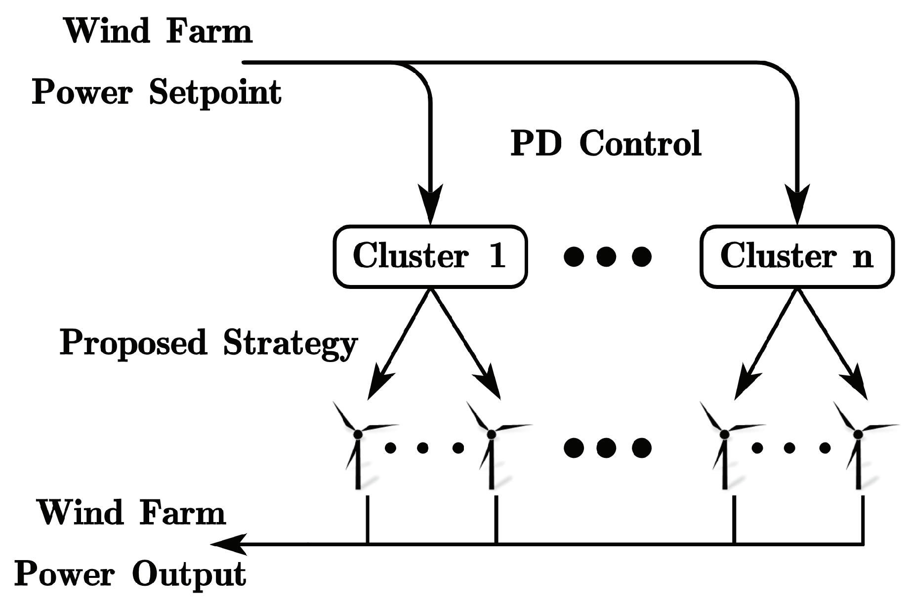The gap between the upper and lower boundaries is used to overcome the power fluctuations caused by inaccurate models and inaccurate wind speed, and a is set at $50\%$ in following simulations. The wind farm control structure is shown in Figure 3.

5. Simulation and Discussion

In this section, the proposed wind farm power controller will be tested to verify the effectiveness. Simulations are carried out with $Matlab$ (2016a, Mathworks, Nedick, MA, USA, 2016). The wind turbines are 5 MW onshore turbines provided in $SimWindFarm$ toolbox. The $SimWindFarm$ toolbox is developed as part of the Aeolus FP7 project, which is aimed at providing a fast wind farm simulation environment for development of wind farm control algorithms. More information about $SimWindFarm$ can be referred from [25,26]. A total of 20 wind turbines are connected together as a wind farm. All WTGSs are differently adjusted in controllers to realize differential regulation of WTGSs characteristics. The simulated wind farm topology is similar as in Figure 1 but with five booster stations. Every four WTGSs are connected to one booster station and form a cluster that can be controlled uniformly. The transmission distances between each WTGS and booster stations are also differently adjusted (detailed WTGS characteristics are listed in

Table 1. Units characteristics (WTGS: wind turbine generator system).

Booster Stations	WTGS Units	Inertial Constant ${\mathit{T}}_{\mathit{i}}$	Distance (km)
1	1	0.179976	3.5
1	2	0.196665	1.5
1	3	0.133947	3
1	4	0.096159	3
2	5	0.108246	1.5
2	6	0.265724	2
2	7	0.101513	0.5
2	8	0.224041	0.5
3	9	0.147858	2
3	10	0.322485	3
3	11	0.095743	3.5
3	12	0.132827	0.5
4	13	0.097878	2
4	14	0.296313	2
4	15	0.090638	0.5
4	16	0.205309	1.5
5	17	0.220674	1
5	18	0.242692	3
5	19	0.096205	1.5
5	20	0.127037	2

).

5.1. Simulation Results

In simulations, the active power distribution from the wind farm to each cluster follows (9), and the clusters will distribute the power demand to each unit by following the proposed power tracking characteristic and power transmission loss based on receding horizon optimization strategy. Only one step prediction is used in the optimization (predictive horizon N is 1). The weight parameter p is set to $0.3$ to achieve the trade-off between the power tracking error and transmission loss. The parameter a in (14) is 50%. The simulated wind farm is controlled under both the proposed strategy and the conventional PD strategy to verify the proposed strategy’s efficiency. The wind farm power output is plotted in Figure 4. The power transmission loss is calculated by following $M=P^2\times D$ and plotted in Figure 5. Curves in red represent the proposed receding horizon strategy and parameters for the conventional PD strategy are drawn in blue. Should be noticed that, simulations are preserved for 200 s in this section. In Figure 4, the tested wind farm power setpoint is a step change polyline including both up and down steps. In the mean time, considering that the amplitude of the step change is large, from the perspective of control theory, the test signal can cover a wide range of the tested wind farm operating range, which can fully stimulate the test system. Thus, only 200 s simulations are reserved in this section as examples.

As shown in Figure 4, the power tracking accuracy under the conventional PD strategy is effectively improved by the proposed receding horizon strategy. The wind farm power output follows the power demand set-point smoothly and accurately, for which the power fluctuation is suppressed effectively. Under the proposed strategy, the wind farm power output follows the power demand quickly at the initial stage and is then stabilized in a short period of time. In Figure 5, the power transmission loss under the proposed strategy is lower than the loss under the PD strategy in the initial 150 s. During the time period between 150 s and 200 s, curves in blue and red cross each other time after time, which shows that the power transmission loss under both strategies are with little difference. For a more detailed comparison, the power tracking absolute error is integrated with time, and the power transmission loss is also integrated as follows:

$$\begin{array}{cc}\hfill P_{IAE}& ={\int }_0^t\left|P_{farm}^{set}(t)-P_{farm}^{out}(t)\right|dt,\hfill \\ \hfill M_I& ={\int }_0^t\left(\sum _{i=1}^n{D}_i\times {(P_i^{out}(t))}^2\right)dt,\hfill \end{array}$$

(18)

and the calculation results are and plotted in Figure 6.

Clearly, the integrated power tracking absolute error and transmission loss under the proposed strategy is lower than the PD strategy. After 200 s simulation, the integrated power tracking absolute error and transmission loss are calculated as

Table 2. $P_{IAE}$ & $M_I$ at 200s (PD: Proportional Distribution).

Control Strategies	${\mathit{P}}_{\mathit{IAE}}$	${\mathit{M}}_{\mathit{I}}$
Conventional PD Strategy	$9.0164\times {10}^6$	$1.2215\times {10}^{16}$
Receding Horizon Strategy	$6.4539\times {10}^6$	$1.1101\times {10}^{16}$

.

As is shown in the table above, the wind farm is improved in both power tracking accuracy and transmission loss under the proposed strategy. The integrated power tracking absolute error is only $60.48\%$ of the conventional one, and the integrated transmission loss is also improved with $91.00\%$ of the conventional strategy. The wind farm can be divided into clusters based on the booster station connections and the WTGS’s power output under the conventional strategy and the proposed strategy in the third cluster are plotted in Figure 7. In this figure, curves in orange represent the wind turbine’s power output under the proposed strategy, and the power outputs under the conventional strategy are drawn in ble.

As is shown in Table 1, in cluster 3, unit 12 has the closest distance from the booster station, unit 11 has the smallest inertial time constant among all four units but the longest distance from the booster station. As for the other units, unit 9 has closer distance and a better power tracking characteristic than unit 10. Thus, as a result, unit 12 takes the leading part when the cluster power demand changes, while unit 11 only takes a basic load because of the conspicuous power transmission loss even though the inertial time constant is small. In the meantime, unit 9 takes a higher power load because of the good characteristic as the first 100 s, and the power output of both unit 9 and 10 shift after 100 s to achieve the trade-off between power tracking accuracy and transmission loss. The simulation result shows that the proposed strategy reaches a satisfactory balance between the wind farm power tracking error and transmission loss. Under the proposed receding horizon active power distribution strategy, both considered characteristics are improved effectively and significantly.

5.2. Discussion

As can be seen in the simulation results, the wind farm is improved by the proposed strategy in both power tracking error and transmission loss, but some problems should still be noticed for further research and application. Firstly, the proposed strategy in this paper is an optimization method based on the receding horizon, and the optimization process goes repeatedly over time. The optimization based method surely can achieve a good control and economy effect, but the solving process still needs to maintain a certain length of time, which is especially limited by computer performance. According to the calculation experiences in simulations, the solving process is usually ended in milliseconds. But considering the data transference, computer performance and signal delay in engineering applications, the proposed strategy could be used in a seconds time scale in a industrial wind farm. Secondly, the optimization problem in this paper is in convex form since both sub cost functions are 2-norm considered parameters and retain convexity after the addition calculation, but clearly the cost function is a nonlinear function. Although the solving of the nonlinear programming problem can be easily achieved by calling the fmincon function provided within Matlab or other related optimization tools, the solving of nonlinear programming problem still need coding implementation when industrial applications are taken into account. Some related references are listed as follows. For optimization problem solving, CVX and Mosek provide convenient, feasible and fast ways by using these toolboxes through Matlab. The introductions and information about these software can be referred to [22,23,24]. When independent programming implementation of optimization solution is needed, the interior point method is a very effective and fast method for solving nonlinear programming. Related references can be referred to [27].

6. Conclusions

In this paper, a wind farm active power receding horizon distribution strategy has been introduced to improve the wind farm power tracking error and transmission loss. For one WTGS, the active power tracking characteristic was modeled as a first-order part in favor of the power tracking error calculation with the unit power set-point changing, and the transmission distance from the analyzed unit to the booster station times the square of unit power output to achieve quantitative characterization of the power transmission loss for one unit. During the power distribution process, the wind farm first divides the power demand to each cluster based on the wind farm topology within the conventional PD strategy, and each cluster makes their own distribution program by a receding horizon optimization strategy in which both tracking error and transmission loss are optimized. The proposed strategy has been tested under a 20 unit wind farm with different characteristics for each unit, which is shown to have a good control effect on both considered characteristics. On the other hand, WTGS in this paper are only considered for power tracking characteristics and transmission loss. Different characteristics could be used when other optimization targets are considered. Limited by the transmission bus connections, WTGSs connected under one booster station can be regarded as one cluster and wind farms in this paper can be divided into clusters according to the topology, and cluster algorithms could be used in different scenarios which is another limitation in this paper. Further research could be concentrated on the fast solving of the proposed optimization strategy for industrial application, or improving the strategy to participate into the primary or secondary frequency regulation of wind turbines and wind farms.

References

1. Lin, Z.; Chen, Z.; Wu, Q.; Yang, S.; Meng, H. Coordinated pitch & torque control of large-scale wind turbine based on Pareto efficiency analysis. Energy 2018, 147, 812–825. [Google Scholar]
2. Kumar, D.; Chatterjee, K. A review of conventional and advanced MPPT algorithms for wind energy systems. Renew. Sustain. Energy Rev. 2016, 55, 957–970. [Google Scholar] [CrossRef]
3. Yin, X.X.; Lin, Y.G.; Li, W.; Gu, Y.J.; Lei, P.F.; Liu, H.W. Adaptive back-stepping pitch angle control for wind turbine based on a new electro-hydraulic pitch system. Int. J. Control 2015, 88, 2316–2326. [Google Scholar] [CrossRef]
4. Lin, Z.; Liu, J.; Niu, Y. Dynamic response regulation of non-linear feedback linearised wind turbine using a two-mass model. IET Control Theory Appl. 2017, 11, 816–826. [Google Scholar] [CrossRef]
5. Lin, Z.; Chen, Z.; Li, X. Regional pole placement and feedback linearization of nonlinear wind turbine control system. In Proceedings of the 2017 American Control Conference (ACC), Seattle, WA, USA, 24–26 May 2017; IEEE: Seattle, WA, USA, 2017; pp. 723–728. [Google Scholar]
6. Rodriguez-Amenedo, J.L.; Arnalte, S.; Burgos, J.C. Automatic generation control of a wind farm with variable speed wind turbines. IEEE Trans. Energy Convers. 2002, 17, 279–284. [Google Scholar] [CrossRef]
7. Hansen, A.D.; Sørensen, P.; Iov, F.; Blaabjerg, F. Centralised power control of wind farm with doubly fed induction generators. Renew. Energy 2006, 31, 935–951. [Google Scholar] [CrossRef]
8. Zhao, H.; Wu, Q.; Guo, Q.; Sun, H.; Xue, Y. Distributed Model Predictive Control of a Wind Farm for Optimal Active Power Control Part I: Clustering-Based Wind Turbine Model Linearization. IEEE Trans. Sustain. Energy 2015, 6, 831–839. [Google Scholar] [CrossRef]
9. Zhao, H.; Wu, Q.; Guo, Q.; Sun, H.; Xue, Y. Distributed Model Predictive Control of a Wind Farm for Optimal Active Power Control Part II: Implementation with Clustering-Based Piece-Wise Affine Wind Turbine Model. IEEE Trans. Sustain. Energy 2015, 6, 840–849. [Google Scholar] [CrossRef]
10. Spudic, V.; Jelavic, M.; Baotic, M. Wind turbine power control for coordinated control of wind farms. In Proceedings of the 18th Internation Conference on Process Control, Tatranska Lomnica, Slovakia, 14–17 June 2011. [Google Scholar]
11. Spudić, V.; Jelavić, M.; Baotić, M. Wind turbine power references in coordinated control of wind farms. Automatika 2011, 52, 82–94. [Google Scholar] [CrossRef]
12. Spudić, V.; Conte, C.; Baotić, M.; Morari, M. Cooperative distributed model predictive control for wind farms. Optim. Control Appl. Methods 2015, 36, 333–352. [Google Scholar] [CrossRef]
13. Guo, Y.; Gao, H.; Wu, Q.; Zhao, H.; Østergaard, J.; Shahidehpour, M. Enhanced voltage control of VSC-HVDC-connected offshore wind farms based on model predictive control. IEEE Trans. Sustain. Energy 2018, 9, 474–487. [Google Scholar] [CrossRef]
14. Guo, Y.; Gao, H.; Xing, H.; Wu, Q.; Lin, Z. Decentralized Coordinated Voltage Control for VSC-HVDC Connected Wind Farms Based on ADMM. IEEE Trans. Sustain. Energy 2018. [Google Scholar] [CrossRef]
15. Huang, S.; Wu, Q.; Guo, Y.; Lin, Z. Bi-level decentralised active power control for large-scale wind farm cluster. IET Renew. Power Gener. 2018, 12, 1486–1492. [Google Scholar] [CrossRef]
16. Vidyanandan, K.; Senroy, N. Primary frequency regulation by deloaded wind turbines using variable droop. IEEE Trans. Power Syst. 2013, 28, 837–846. [Google Scholar] [CrossRef]
17. Sun, Y.Z.; Zhang, Z.S.; Li, G.J.; Lin, J. Review on frequency control of power systems with wind power penetration. In Proceedings of the 2010 International Conference on Power System Technology (POWERCON), Hangzhou, China, 24–28 October 2010; IEEE: Piscataway, NJ, USA, 2010; pp. 1–8. [Google Scholar]
18. Natsheh, E.M.; Albarbar, A.; Yazdani, J. Modeling and control for smart grid integration of solar/wind energy conversion system. In Proceedings of the 2011 2nd IEEE PES International Conference and Exhibition on Innovative Smart Grid Technologies, Manchester, UK, 5–7 December 2011; pp. 1–8. [Google Scholar] [CrossRef]
19. Yao, E.; Wang, H.; Wang, L.; Xi, G.; Marechal, F. Multi-objective optimization and exergoeconomic analysis of a combined cooling, heating and power based compressed air energy storage system. Energy Convers. Manag. 2017, 138, 199–209. [Google Scholar] [CrossRef]
20. Cai, W.; Liu, F.; Zhang, H.; Liu, P.; Tuo, J. Development of dynamic energy benchmark for mass production in machining systems for energy management and energy-efficiency improvement. Appl. Energy 2017, 202, 715–725. [Google Scholar] [CrossRef]
21. Cai, W.; Liu, F.; Xie, J.; Zhou, X.N. An energy management approach for the mechanical manufacturing industry through developing a multi-objective energy benchmark. Energy Convers. Manag. 2017, 132, 361–371. [Google Scholar] [CrossRef]
22. Mosek, A. The MOSEK Optimization Toolbox for MATLAB Manual; Mosek ApS: København, Denmark, 2015. [Google Scholar]
23. Grant, M.; Boyd, S. CVX: Matlab Software for Disciplined Convex Programming, version 2.1. 2014. Available online: http://cvxr.com/cvx (accessed on 1 March 2014).
24. Grant, M.; Boyd, S. Graph implementations for nonsmooth convex programs. In Recent Advances in Learning and Control; Blondel, V., Boyd, S., Kimura, H., Eds.; Lecture Notes in Control and Information Sciences; Springer: Berlin/Heidelberg, Germany, 2008; pp. 95–110. [Google Scholar]
25. Grunnet, J.D.; Soltani, M.; Knudsen, T.; Kragelund, M.; Bak, T. Aeolus Toolbox for Dynamic Wind Farm Model, Simulation and Control. In Proceedings of the 2010 European Wind Energy Conference, Warsaw, Poland, 20–23 April 2010. [Google Scholar]
26. SimWindFarm Toolbox. 2017. Available online: http://www.ict-aeolus.eu/SimWindFarm/index.html (accessed on 1 December 2017).
27. Boyd, S.; Vandenberghe, L. Convex Optimization; Cambridge University Press: Cambridge, UK, 2004. [Google Scholar]
Figure 1. Wind farm topology. High voltage (HV), medium voltage (MV), and wind turbine generator system (WTGS).
Processes 06 00259 g001
Figure 2. Wind turbine power tracking dynamic characteristic.
Processes 06 00259 g002
Figure 3. Wind farm control structure. Proportional distribution (PD).
Processes 06 00259 g003
Figure 4. Wind farm active power output comparison.
Processes 06 00259 g004
Figure 5. Wind farm transmission loss comparison.
Processes 06 00259 g005
Figure 6. Integrated wind farm power tracking absolute error and integrated transmission loss.
Processes 06 00259 g006
Figure 7. Cluster 3 units power output comparison.
Processes 06 00259 g007