Approximating Nonlinear Relationships for Optimal Operation of Natural Gas Transport Networks


Abstract
1. Introduction
2. Common Natural Gas Transportation Model
2.1. Network Topography
2.2. Gas Flow Model
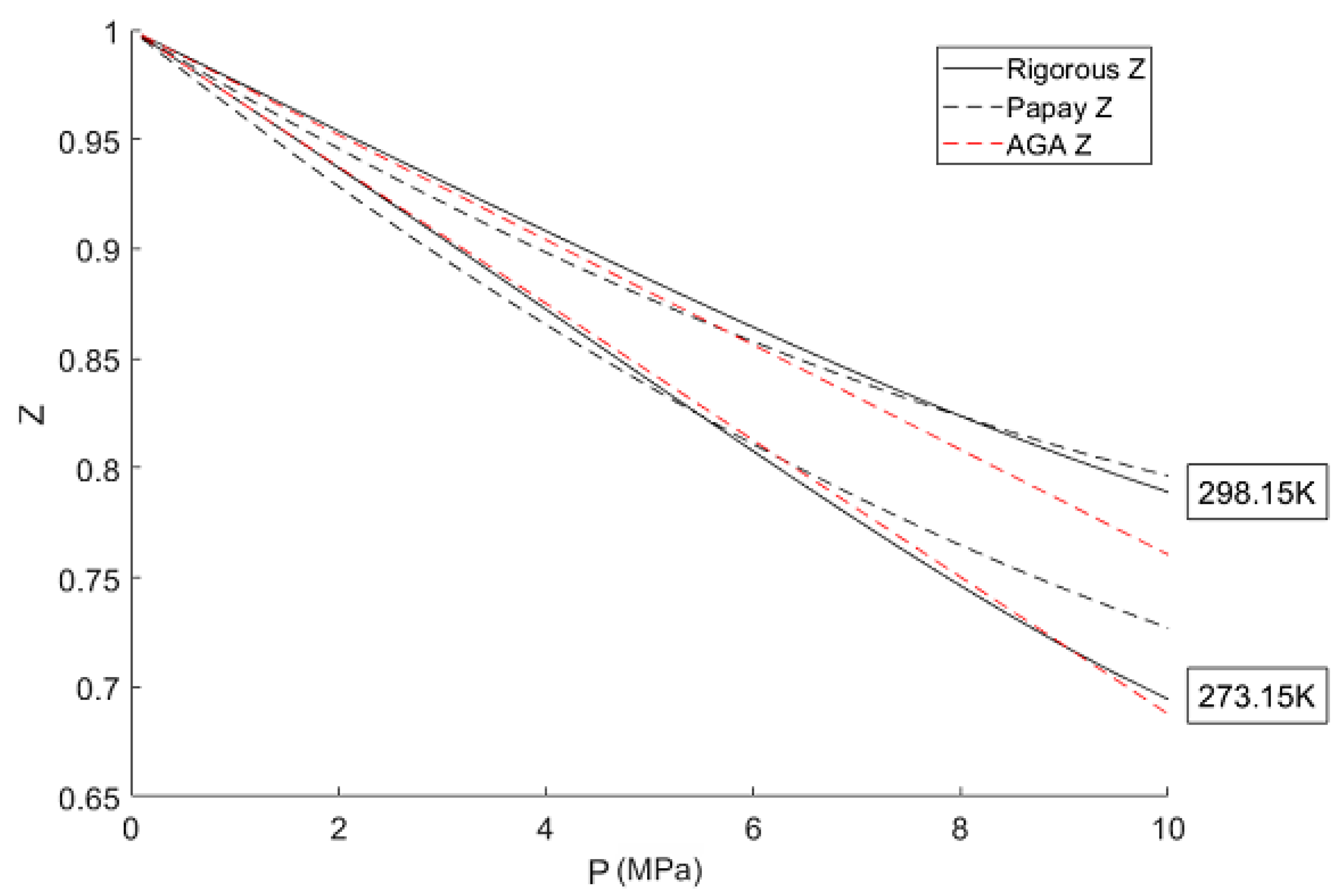
2.2.1. Compressibility Factor
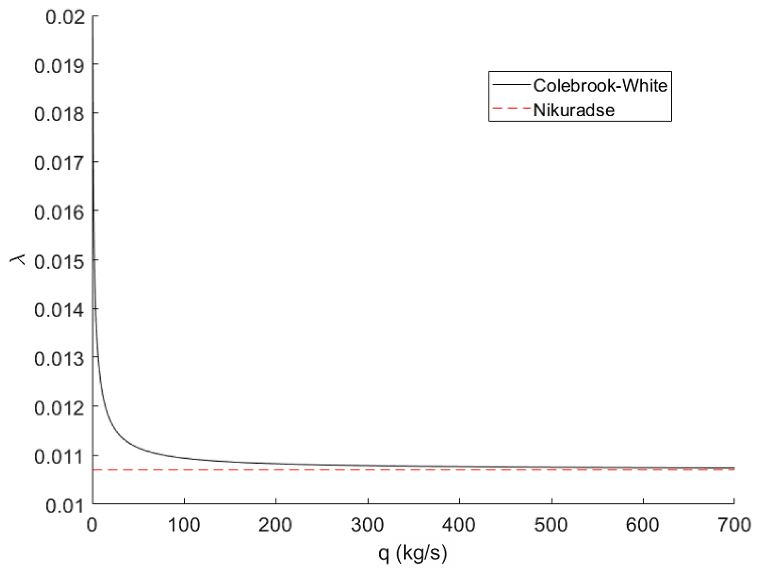
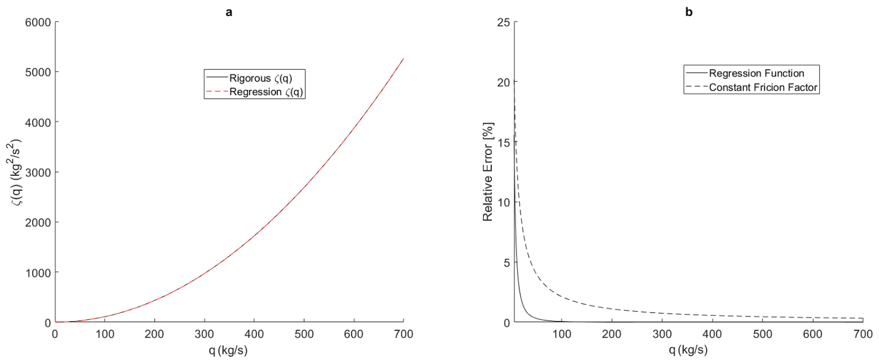
2.2.2. Friction Factor
2.3. Compressor Equations
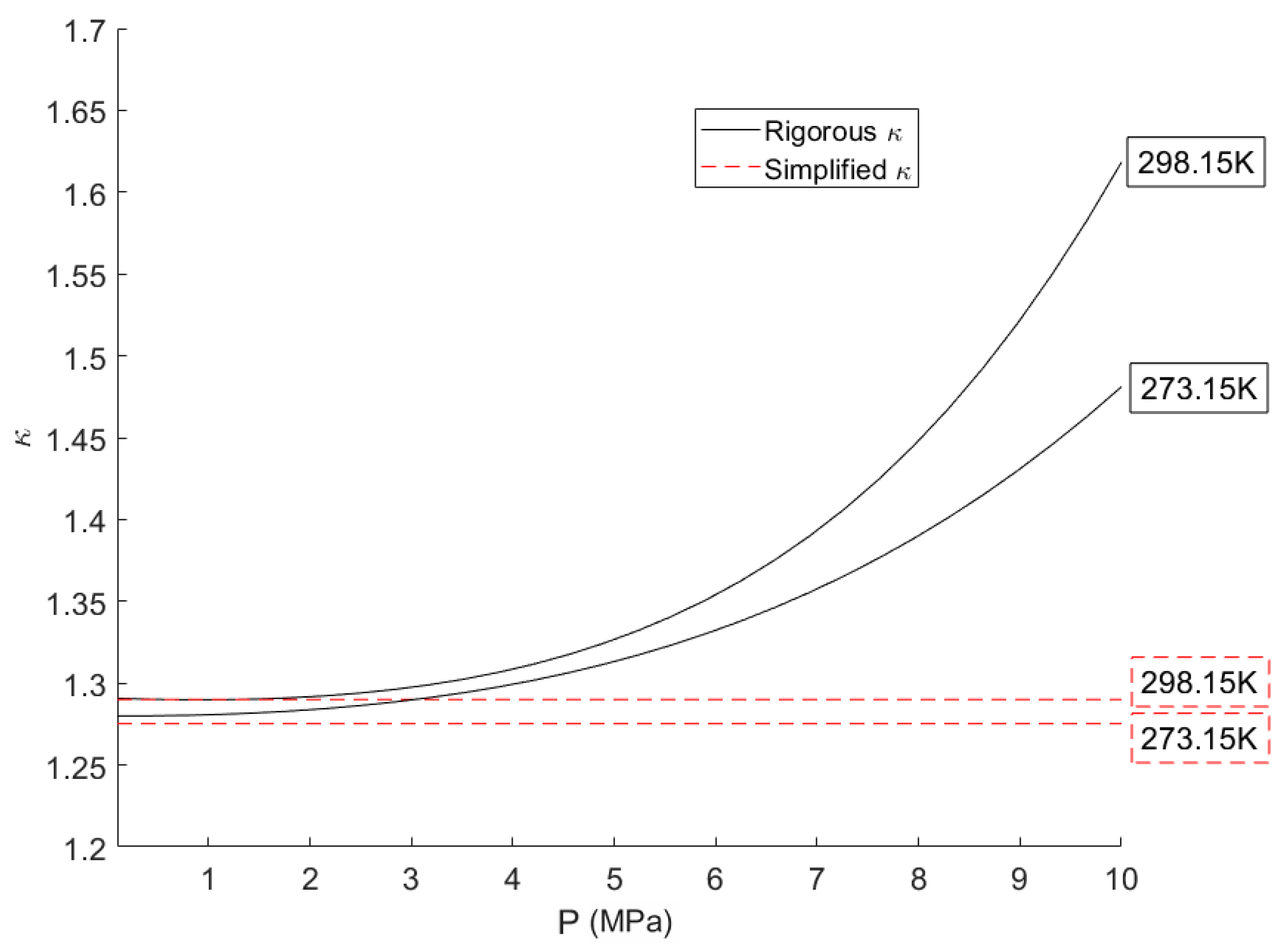
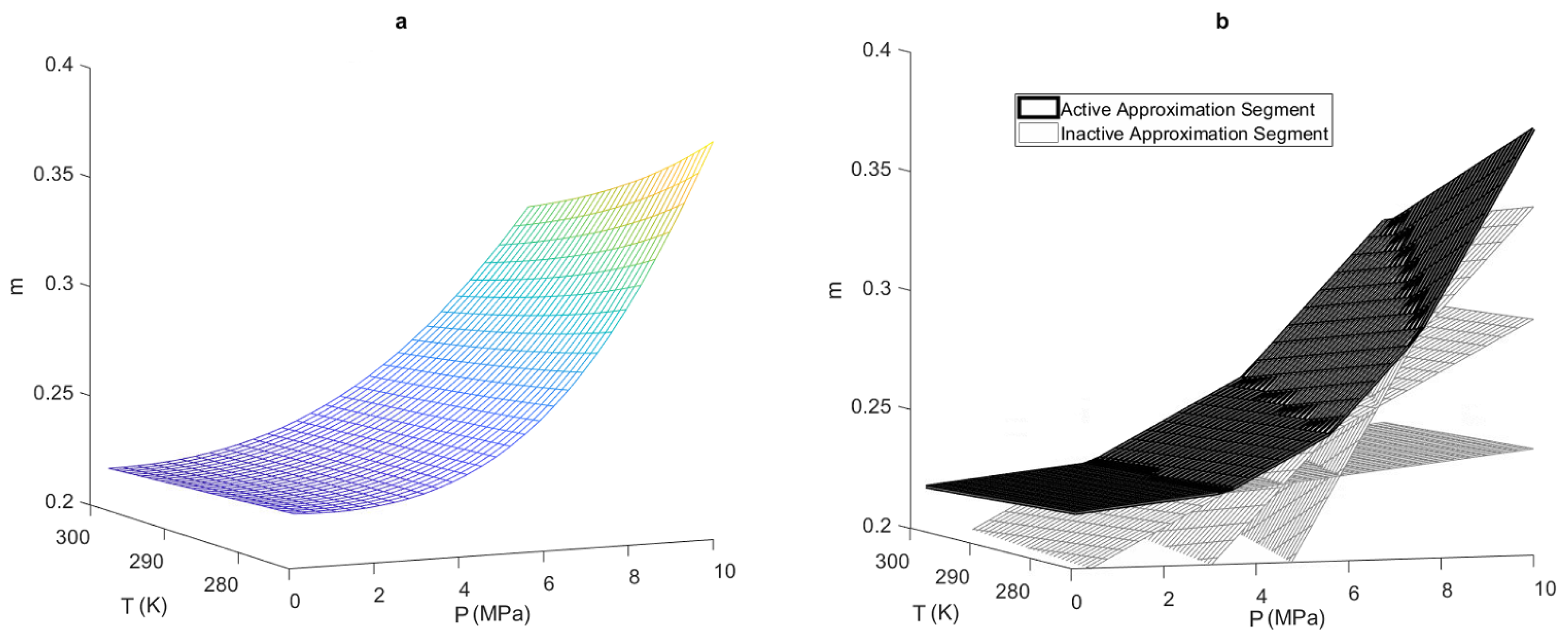
2.3.1. Isentropic Exponent
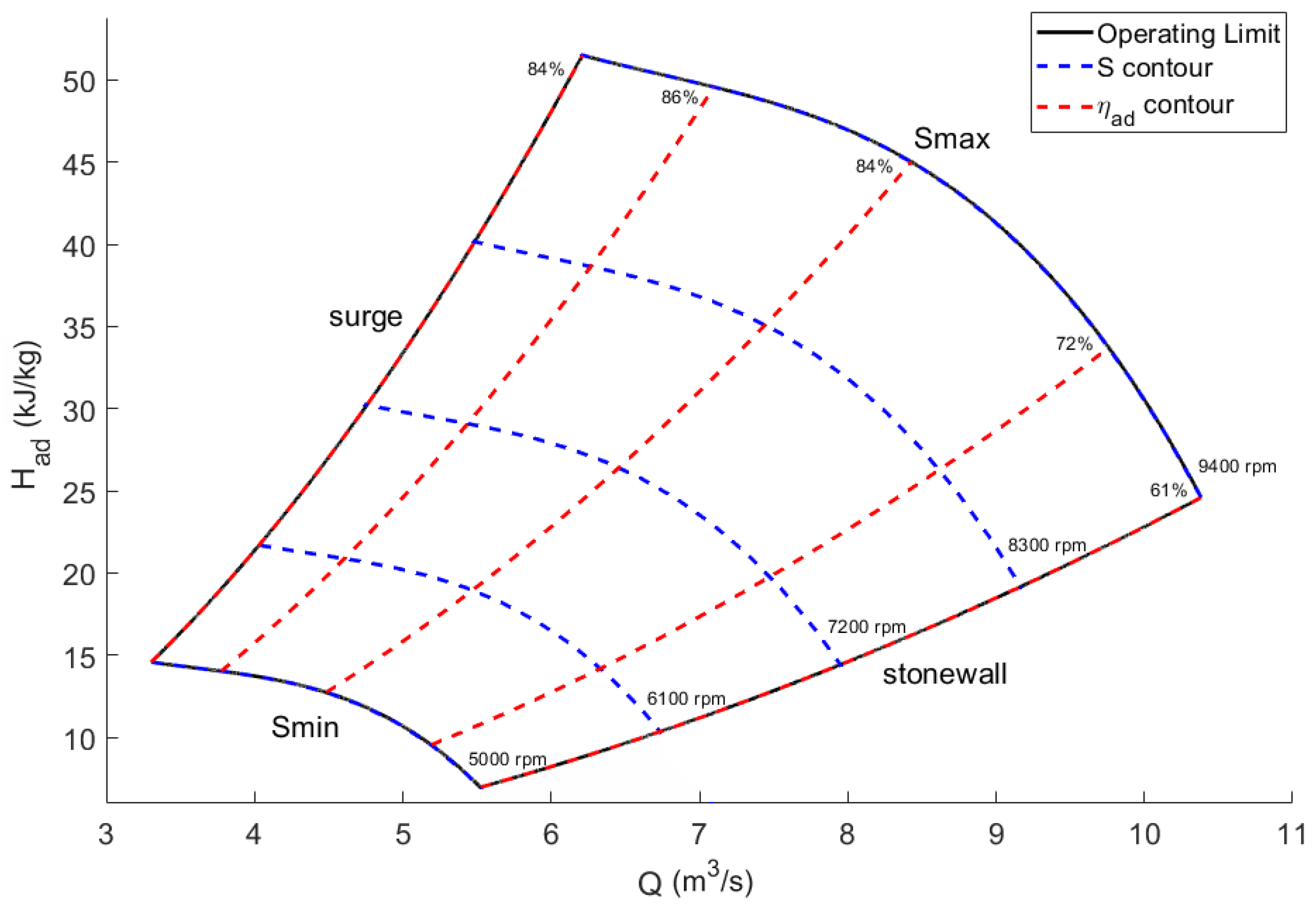
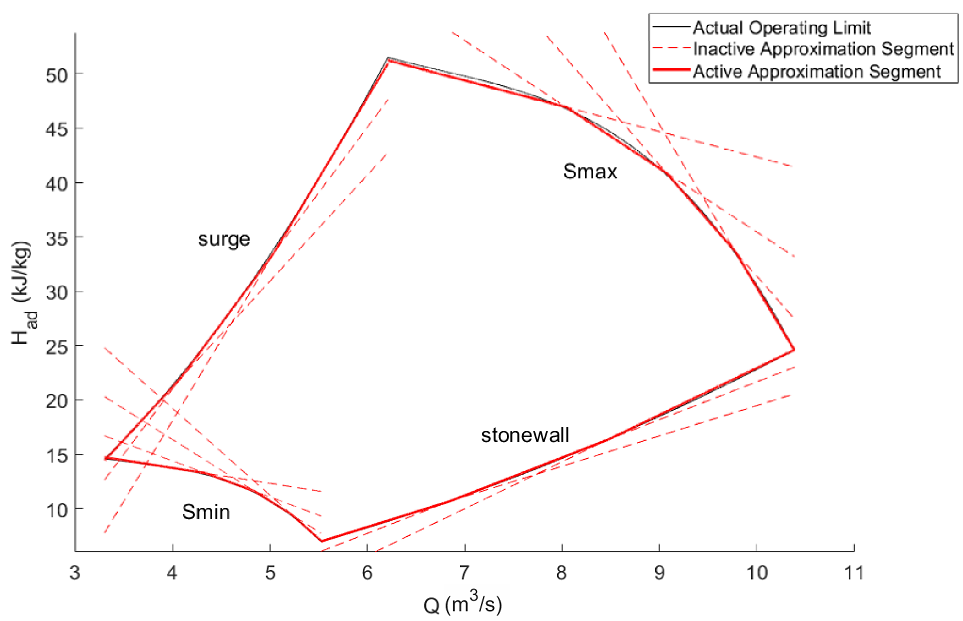
2.3.2. Compressor Operating Envelop
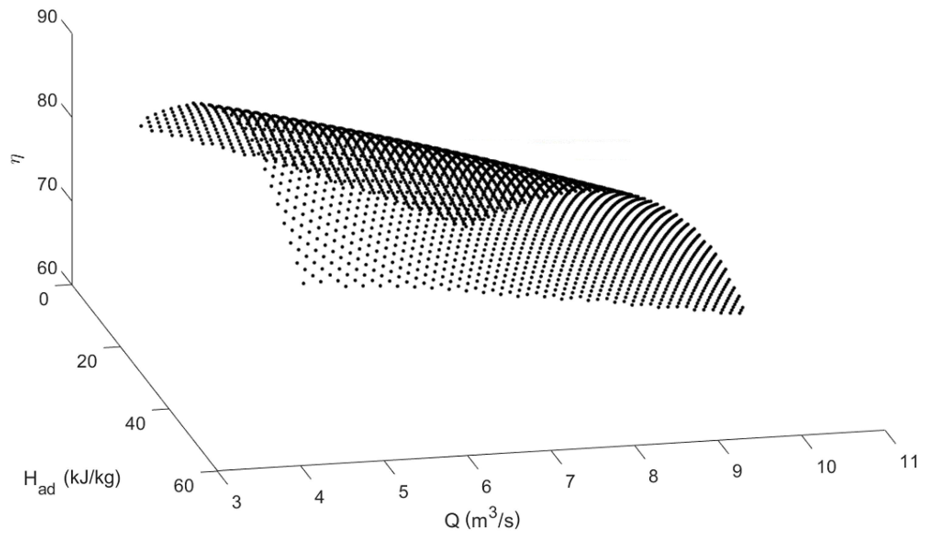
2.3.3. Compressor Efficiency
2.4. Common FCMP Model
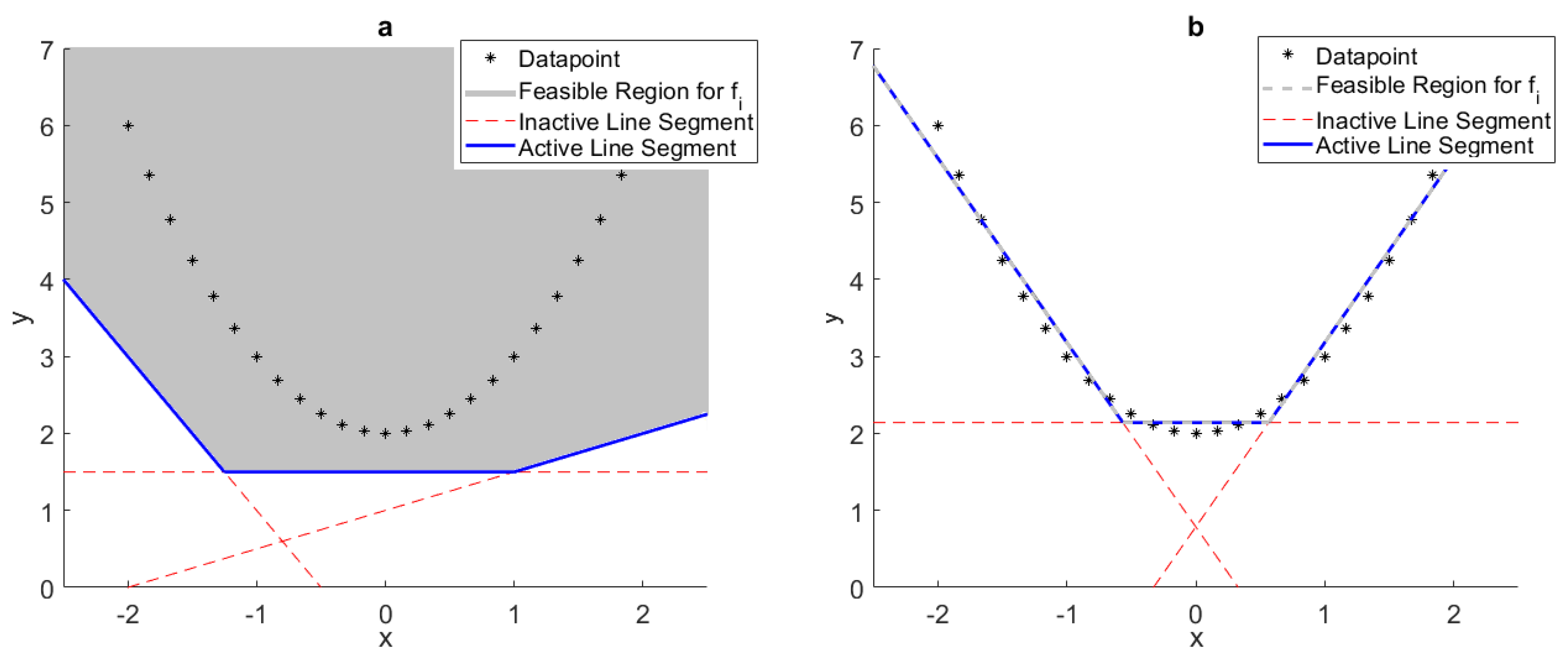
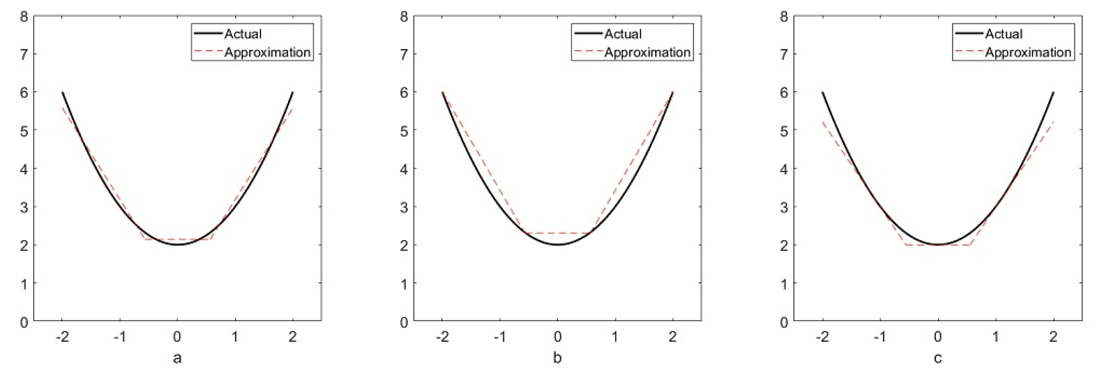
3. Optimal Piecewise-Linear Function Generation
- Decide what is an acceptable amount of maximum relative error between the piecewise-linear function being generated and the relationship being approximated, this is the stopping criteria . Typically, 1% is appropriate.
- Start with and , where M is some relatively small number of data points equally dispersed over the approximation domain. Solve the MILP for the piecewise-linear function, .
- Calculate the maximum error between and the entire dataset of the relationship being approximated, .
- Increase m to , and solve the MILP for .
- Calculate .
- Iterate Steps 4 and 5 until the change in is less than 1% for two consecutive iterations, then move to Step 7. If the MILP becomes intractable before this, move to Step 7.
- If the smallest is less than , or has changed less than 1% for two consecutive increases in p, terminate, the corresponding is either an acceptable approximation or as good as the PLFG method is likely to yield. Else, increase p to , reinitialize , and return to Step 4. If the MILP becomes intractable before meeting the stopping criteria, terminate and consider breaking up the domain of approximation.
4. Relationship Approximation
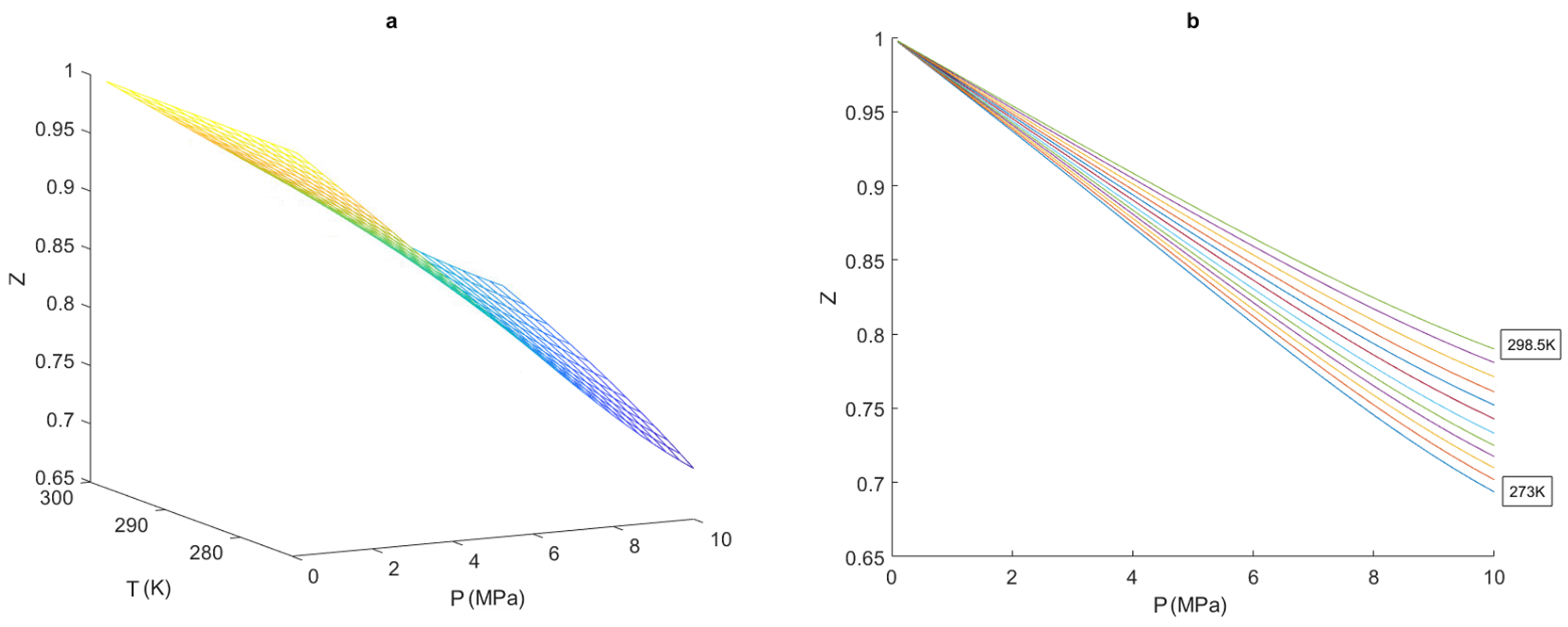
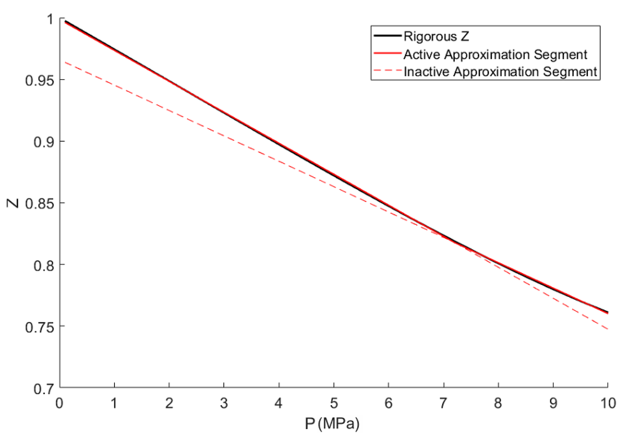
4.1. Compressibility Factor
4.2. Friction Factor
4.3. Isentropic Exponent
4.4. Compressor Model
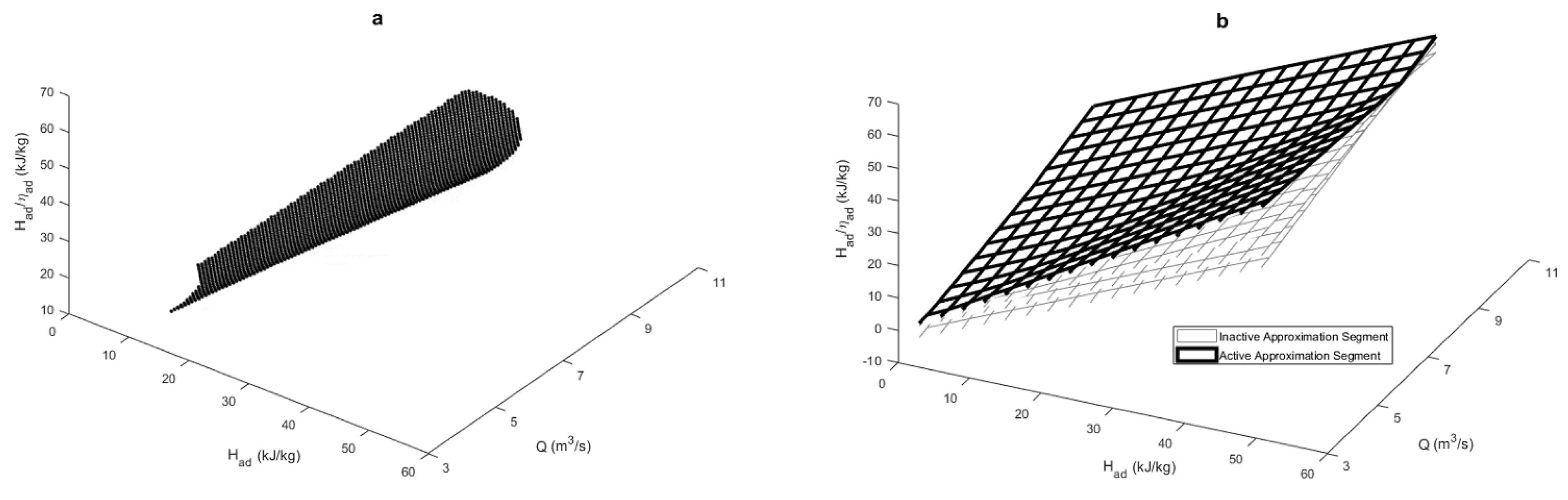
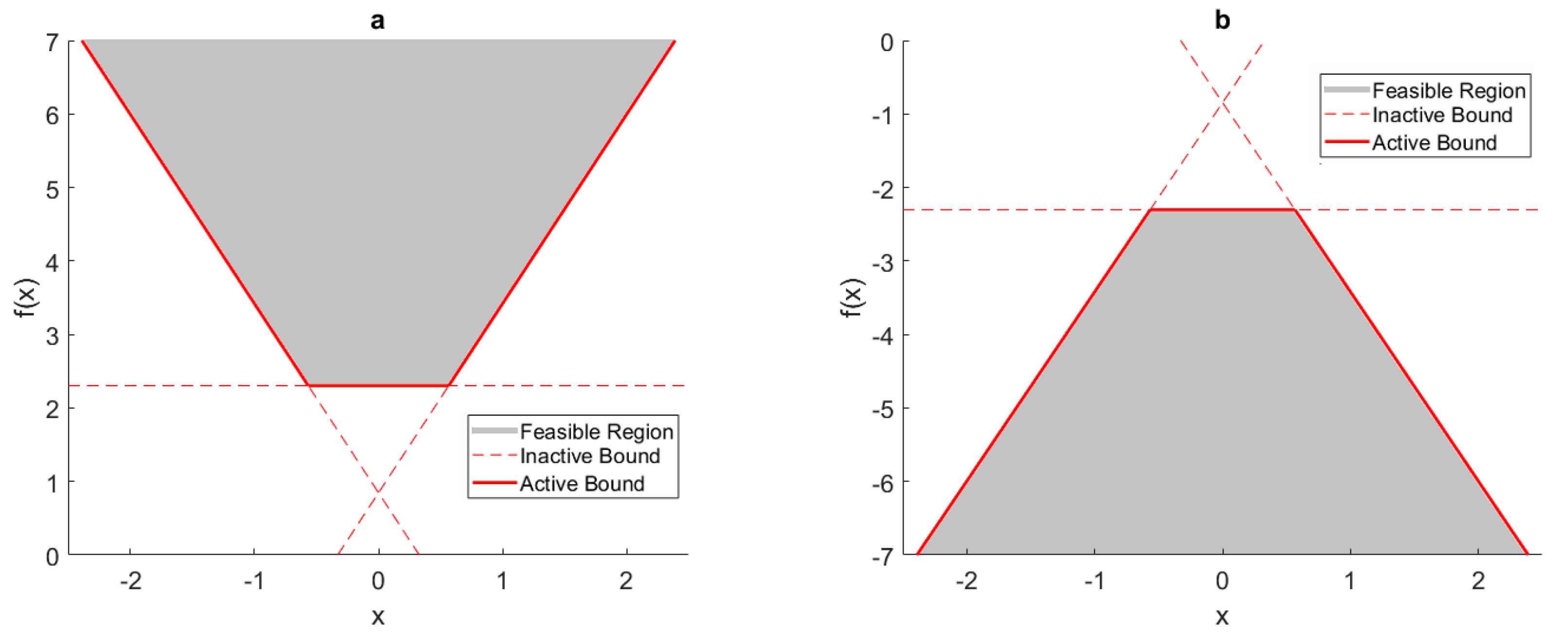
4.4.1. Compressor Operating Envelop
4.4.2. Compressor Efficiency
5. FCMP Model with Novel Relationship Approximations
5.1. Compressibility Factor
5.2. Friction Factor
5.3. Isentropic Exponent
5.4. Compressor Operating Envelop
5.5. Compressor Efficiency
6. Case Study
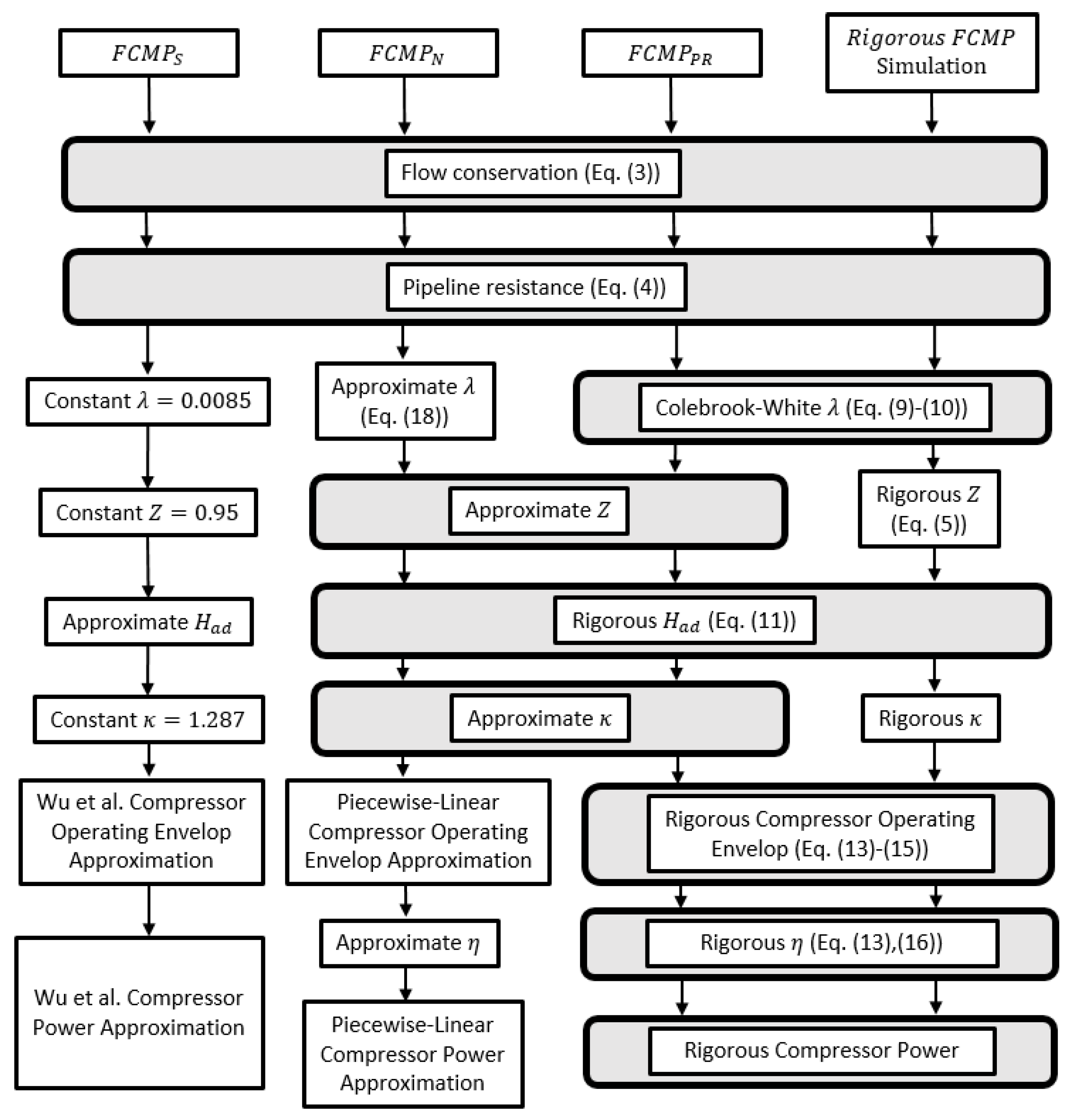
6.1. FCMP Models
- The pressure of the first node is set as the first node pressure from the optimal solution.
- If the next arc is a pipe section, then the pressure of the next node is calculated using the pipeline resistance equation, where Z and are calculated using their rigorous relations. Else, move to Step 3.
- The next arc is a compressor station, so the outlet pressure is set as the outlet pressure from the optimal solution. The simulated compressor fuel cost is then calculated using the rigorous calculations for Z, , , and so that a theoretically exact fuel cost is obtained.
- Return to Step 2 and iterate until all node pressures and compressor station fuel costs are calculated.
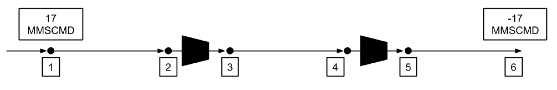
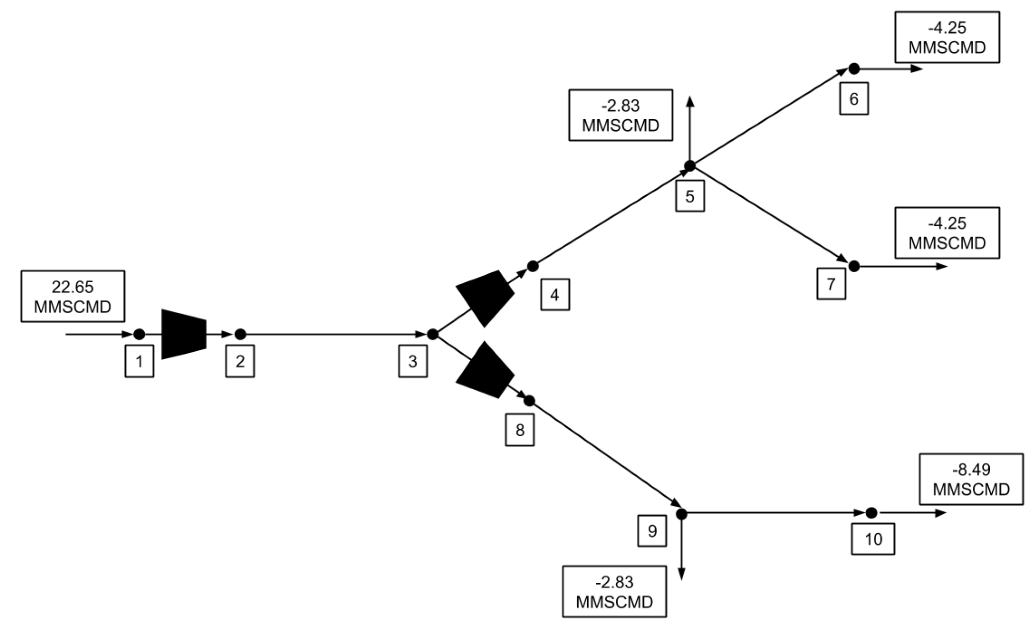
6.2. Example 1
6.3. Example 2
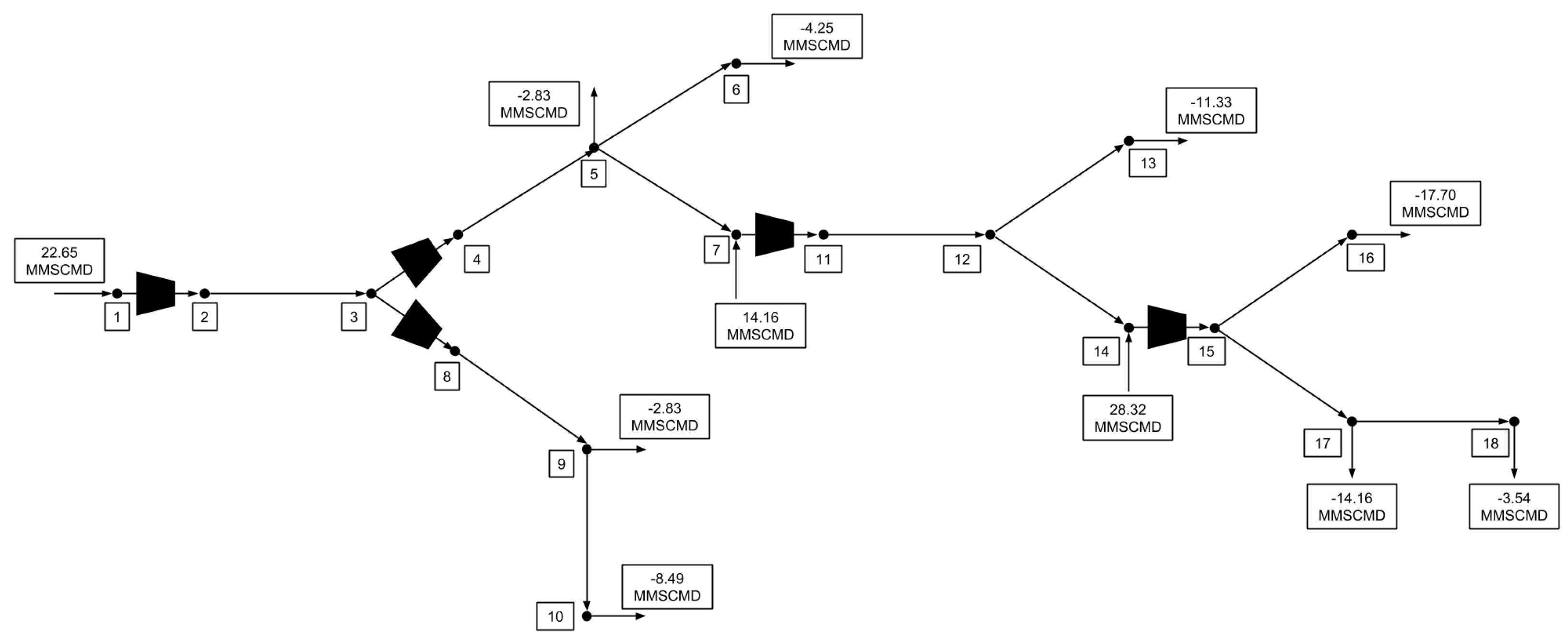
6.4. Example 3
7. Conclusions and Future Work
Author Contributions
Funding
Conflicts of Interest
Abbreviations
| FCMP | Fuel Cost Minimization Problem |
| NLP | Nonlinear Program |
| MINLP | Mixed-Integer Nonlinear Program |
| PLFG | Piecewise-Linear Function Generation |
| MILP | Mixed-Integer Linear Program |
Appendix A. Novel FCMP Model (FCMPN)
Appendix B. Simplified FCMP Model (FCMPS)
Appendix C. Rigorous FCMP Model (FCMPR)
References
- IEA. World Energy Outlook 2016; International Energy Agency: Paris, France, 2016; p. 684. [Google Scholar]
- Schroeder, D. Hydraulic analysis in the natural gas industry. In Advances in Industrial Engineering Applications and Practice I; International Journal of Industrial Engineering: Houston, TX, USA, 1996; pp. 960–965. [Google Scholar]
- Ríos-Mercado, R.Z.; Borraz-Sánchez, C. Optimization problems in natural gas transportation systems: A state-of-the-art review. Appl. Energy 2015, 147, 536–555. [Google Scholar] [CrossRef]
- Tawarmalani, M.; Sahinidis, N.V. A polyhedral branch-and-cut approach to global optimization. Math. Program. 2005, 103, 225–249. [Google Scholar] [CrossRef]
- Sahinidis, N.V. BARON 17.8.9: Global Optimization of Mixed-Integer Nonlinear Programs, User’s Manual; BARON Software: Pittsburgh, PA, USA, 2017. [Google Scholar]
- Gleixner, A.; Eifler, L.; Gally, T.; Gamrath, G.; Gemander, P.; Gottwald, R.L.; Hendel, G.; Hojny, C.; Koch, T.; Miltenberger, M.; et al. The SCIP Optimization Suite 5.0; ZIB-Report 17-61; Zuse Institute: Berlin, Germany, 2017. [Google Scholar]
- Schmidt, M.; Steinbach, M.C.; Willert, B.M. High detail stationary optimization models for gas networks. Optim. Eng. 2015, 16, 131–164. [Google Scholar] [CrossRef]
- Misra, S.; Fisher, M.W.; Backhaus, S.; Bent, R.; Chertkov, M. Optimal Compression in Natural Gas Networks: A Geometric Programming Approach. IEEE Trans. Control Netw. Syst. 2015, 2, 47–56. [Google Scholar] [CrossRef]
- Borraz-Sánchez, C.; Haugland, D. Minimizing fuel cost in gas transmission networks by dynamic programming and adaptive discretization. Comput. Ind. Eng. 2011, 61, 364–372. [Google Scholar] [CrossRef]
- Martin, A.; Moller, M.; Moritz, S. Mixed Integer Models for the Stationary Case of Gas Network Optimization. Math. Program. 2006, 105, 563–582. [Google Scholar] [CrossRef]
- Wong, P.; Larson, R. Optimization of Natural-Gas Pipeline Systems Via Dynamic Programming. IEEE Trans. Autom. Control 1968, 13, 475–481. [Google Scholar] [CrossRef]
- Wolf, D.D.; Smeers, Y. The Gas Transmission Problem Solved by an Extension of the Simplex Algorithm. Manag. Sci. 2000, 46, 1454–1465. [Google Scholar] [CrossRef]
- Borraz-Sanchez, C.; Rios-Mercado, R.Z. Improving the Operation of Pipeline Systems on Cyclic Structures by Tabu Search. Comput. Chem. Eng. 2009, 33, 58–64. [Google Scholar] [CrossRef]
- Flores-Villarreal, H.; Rios-Mercado, R. Computational Experience With a GRG Method for Minimizing Fuel Consumption on Cyclic Natural Gas Networks. In Computational Methods in Circuits System Applications; World Scientific and Engineering Academy and Society Press: Cambridge, UK, 2003; pp. 90–94. [Google Scholar]
- Chebouha, A.; Yalaoui, F.; Smati, A.; Younsi, K.; Tairi, A. Optimization of Natural Gas Pipeline Transportation Using Ant Colony Optimization. Comput. Oper. Res. 2009, 36, 1916–1923. [Google Scholar] [CrossRef]
- ISO-12213-2. Natural Gas—Calculation of Compression Factor—Part 2: Calculation Using Molar-Composition Analysis; Technical Report; International Organization for Standardization: Geneva, Switzerland, 2006. [Google Scholar]
- Westhoff, M.A. Using Operating Data at Natural Gas Pipelines; Technical Report; Colorado Interstate Gas Company: Houston, TX, USA, 2004. [Google Scholar]
- Coelho, P.; Pinho, C. Considerations About Equations for Steady State Flow in Natural Gas Pipelines. J. Braz. Soc. Mech. Sci. Eng. 2007, 29, 262–273. [Google Scholar] [CrossRef]
- About U.S. Natural Gas Pipelines—Transporting Natural Gas. Available online: https://www.eia.gov/naturalgas/archive/analysis_publications/ngpipeline/interstate.html (accessed on 27 March 2018).
- Kelkar, M. Natural Gas Production Engineering; PennWell Books: Tulsa, OK, USA, 2008; Chapter Gas Compression; pp. 445–464. [Google Scholar]
- Maric, I.; Galovic, A.; Smuc, T. Calculation of natural gas isentropic exponent. Flow Measur. Instrum. 2005, 16, 13–20. [Google Scholar] [CrossRef]
- Mokhatab, S.; Poe, W.A.; Speight, J.G. (Eds.) Handbook of Natural Gas Transmission and Processing; Elsevier: Amsterdam, The Netherlands, 2006; Chapter Natural Gas Compression; pp. 295–322. [Google Scholar]
- Wu, S.; Rios-Mercado, R.; Boyd, E.; Scott, L. Model Relaxations for the Fuel Cost Minimization of Steady-State Gas Pipeline Networks. Math. Comput. Model. 2000, 31, 197–220. [Google Scholar] [CrossRef]
- Wu, X.; Li, C.; Jia, W.; He, Y. Optimal Operation of Trunk Natural Gas Pipelines Via an Inertia-Adaptive Particle Swarm Optimization Algorithm. J. Nat. Gas Sci. Eng. 2014, 21, 10–18. [Google Scholar] [CrossRef]
- Nørstebø, V.S.; Rømo, F.; Hellemo, L. Using operations research to optimise operation of the Norwegian natural gas system. J. Nat. Gas Sci. Eng. 2010, 2, 153–162. [Google Scholar] [CrossRef]
- Tabkhi, F.; Pibouleau, L.; Hernandez-Rodriguez, G.; Azzaro-Pantel, C.; Domenech, S. Improving the Performance of Natural Gas Pipeline Networks Fuel Consumption Minimization Problems; Wiley Interscience: Hoboken, NJ, USA, 2009. [Google Scholar]
- Rios-Mercado, R.Z.; Kim, S.; Boyd, E.A. Efficient operation of natural gas transmission systems: A network-based heuristic for cyclic structures. Comput. Oper. Res. 2006, 33, 2323–2351. [Google Scholar] [CrossRef]
- Camponogara, E.; Nazari, L. Models and Algorithms for Optimal Piecewise-Linear Function Approximation. Math. Probl. Eng. 2015, 2015. [Google Scholar] [CrossRef]
- Codas, A.; Camponogara, E. Mixed-integer linear optimization for optimal lift-gas allocation with well-separator routing. Eur. J. Oper. Res. 2011, 217, 222–231. [Google Scholar] [CrossRef]
- Carrión, M.; Arroyo, J.M. A Computationally Efficient Mixed-Integer Linear Formulation for the Thermal Unit Commitment Problem. IEEE Trans. Power Syst. 2006, 21, 1371–1378. [Google Scholar] [CrossRef]
- Toriello, A.; Vielma, J. Fitting piecewise linear continuous functions. Eur. J. Oper. Res. 2012, 219, 86–95. [Google Scholar] [CrossRef]
- GasLib. Available online: http://gaslib.zib.de/ (accessed on 25 September 2018).
- GAMS Development Corporation. General Algebraic Modeling System (GAMS) Release 25.1.1; GAMS Development Corporation: Washington, DC, USA, 2018. [Google Scholar]
- The MathWorks Inc. MATLAB and Statistics Toolbox Release 2018a; The MathWorks Inc.: Natick, MA, USA, 2018. [Google Scholar]


| Symbol | Description | Unit |
|---|---|---|
| q | Mass flow rate | kg s |
| P | Pressure | MPa |
| T | Temperature | K |
| L | Length | m |
| D | Diameter | m |
| A | Cross-sectional area | m |
| Friction coefficient | - | |
| Z | Compressibility factor | - |
| R | Gas constant | J mol K |
| Molecular weight | kg mol | |
| B | Second virial coefficient | m kmol |
| Molar density | kmol m | |
| K | Size parameter | m kmol |
| Compressibility factor coefficient | - | |
| Compressibility factor constant | - | |
| Critical temperature | K | |
| Critical pressure | MPa | |
| Absolute roughness | m | |
| Reynolds Number | - | |
| Gas dynamic viscosity | Pa s | |
| Specific change in adiabatic enthalpy | J kg | |
| Isentropic exponent | - | |
| Q | Volumetric flow rate | ms |
| S | Compressor speed | rpm |
| Compressor speed limit | rpm | |
| Compressor throughput/speed limit | msrpm | |
| Adiabatic efficiency | - |
| Symbol | Description | Unit |
|---|---|---|
| Compressibility factor binary variable | - | |
| , | Compressibility factor line coefficients | MPa, - |
| Compressibility factor sufficiently large number | - | |
| , | Friction factor regression coefficients | -, kg s |
| m binary variable | - | |
| , , | m plane coefficients | K, MPa, - |
| , | Stonewall limit line coefficients | kJ-s kg-m, kJ kg |
| , | Smax limit line coefficients | kJ-s kg-m, kJ kg |
| Smin limit binary variable | - | |
| , | Smin limit line coefficients | kJ-s kg-m, kJ kg |
| Smin limit sufficiently large number | kJ kg | |
| Smin limit bound variable | kJ kg | |
| Surge limit binary variable | - | |
| , | Surge limit line coefficients | kJ-s kg-m, kJ kg |
| Surge limit sufficiently large number | kJ kg | |
| Surge limit bound variable | kJ kg | |
| , , | plane coefficients | kJ-s kg-m, -, kJ kg |
| Variable | Optimization | Simulation | Optimization | Simulation | Optimization | Simulation |
| (MPa) | 4.99 | 4.99 | 5.01 | 5.01 | 5.01 | 5.01 |
| 4.47 | 4.37 | 4.39 | 4.39 | 4.39 | 4.39 | |
| 4.87 | 4.87 ** | 4.92 | 4.92 | 4.92 | 4.92 | |
| 4.33 | 4.22 | 4.28 | 4.29 | 4.28 | 4.29 | |
| 4.70 | 4.70 ** | 4.80 | 4.80 | 4.80 | 4.80 | |
| 4.14 | 4.02 * | 4.14 | 4.14 | 4.14 | 4.14 | |
| Fuel Cost (kJ s) | 39.76 | 44.88 *** | 47.31 | 47.33 | 47.58 | 47.28 |
| % Diff | 11.41% | 0.05% | 0.61% | |||
| Solution Time (s) | 0.32 s | 1.26 s | 5.97 s | |||
| # of Constraints | 31 | 123 | 86 | |||
| # of Continuous Variables | 23 | 71 | 68 | |||
| # of Discrete Variables | 2 | 34 | 20 | |||
| Variable | Optimization | Simulation | Optimization | Simulation | Optimization | Simulation |
| (MPa) | 4.26 | 4.26 | 4.38 | 4.38 | 4.38 | 4.38 |
| 4.53 | 4.53 | 4.69 | 4.69 | 4.69 | 4.69 | |
| 3.42 | 3.15 | 3.37 | 3.38 | 3.38 | 3.38 | |
| 3.79 | 3.79 ** | 3.79 | 3.79 | 3.79 | 3.79 | |
| 3.49 | 3.42 | 3.42 | 3.42 | 3.42 | 3.42 | |
| 3.45 | 3.36 | 3.36 | 3.36 | 3.36 | 3.36 | |
| 3.45 | 3.36 | 3.36 | 3.36 | 3.36 | 3.36 | |
| 3.79 | 3.79 ** | 3.79 | 3.79 | 3.79 | 3.79 | |
| 3.49 | 3.42 | 3.42 | 3.42 | 3.42 | 3.42 | |
| 3.31 | 3.18 | 3.18 | 3.18 | 3.18 | 3.18 | |
| Fuel Cost (kJ s) | 56.55 | 79.51 *** | 58.47 | 57.88 | 58.17 | 57.72 |
| % Diff | 28.87% | 1.02% | 0.78% | |||
| Solution Time (s) | 1.03 s | 1.88 s | 54.26 s | |||
| # of Constraints | 50 | 197 | 146 | |||
| # of Continuous Variables | 30 | 115 | 115 | |||
| # of Discrete Variables | 3 | 54 | 33 | |||
| Variable | Optimization | Simulation | Optimization | Simulation | Optimization | Simulation |
| (MPa) | 4.26 | 4.26 | 4.46 | 4.46 | 4.45 | 4.45 |
| 4.53 | 4.53 ** | 4.81 | 4.81 | 4.80 | 4.80 | |
| 3.42 | 3.15 | 3.56 | 3.56 | 3.54 | 3.54 | |
| 3.79 | 3.79 ** | 4.01 | 4.01 | 4.01 | 4.01 | |
| 3.49 | 3.42 | 3.66 | 3.66 | 3.66 | 3.66 | |
| 3.45 | 3.36 | 3.60 | 3.60 | 3.60 | 3.60 | |
| 3.45 | 3.36 | 3.60 | 3.60 | 3.60 | 3.60 | |
| 3.79 | 3.79 ** | 4.01 | 4.01 | 3.98 | 3.98 | |
| 3.49 | 3.42 | 3.66 | 3.66 | 3.63 | 3.63 | |
| 3.31 | 3.18 | 3.44 | 3.44 | 3.41 | 3.41 | |
| 3.66 | 3.66 ** | 3.84 | 3.84 | 3.84 | 3.84 | |
| 2.76 | 2.49 | 2.75 | 2.76 | 2.75 | 2.76 | |
| 2.32 | 1.85 | 2.19 | 2.19 | 2.19 | 2.19 | |
| 2.59 | 2.26 | 2.55 | 2.55 | 2.55 | 2.55 | |
| 2.76 | 2.76 ** | 2.77 | 2.77 | 2.77 | 2.77 | |
| 1.49 | 0.85 | 0.88 | 0.88 | 0.88 | 0.88 | |
| 1.49 | 0.85 | 0.88 | 0.88 | 0.88 | 0.88 | |
| 1.42 | 0.65 * | 0.69 | 0.69 | 0.69 | 0.69 | |
| 2 | 1 | 1 | ||||
| 1 | 1 | 1 | ||||
| 1 | 1 | 1 | ||||
| 2 | 1 | 1 | ||||
| 4 | 3 | 3 | ||||
| Fuel Cost (kJ s) | 98.21 | 187.08 *** | 123.02 | 122.26 | 123.74 | 122.77 |
| % Diff | 47.50% | 0.62% | 0.79% | |||
| Solution Time (s) | 3.99 s | 8.21 s | 994.98 s | |||
| # of Constraints | 88 | 345 | 266 | |||
| # of Continuous Variables | 68 | 205 | 211 | |||
| # of Discrete Variables | 5 | 94 | 59 | |||
© 2018 by the authors. Licensee MDPI, Basel, Switzerland. This article is an open access article distributed under the terms and conditions of the Creative Commons Attribution (CC BY) license (http://creativecommons.org/licenses/by/4.0/).
Share and Cite
Kazda, K.; Li, X. Approximating Nonlinear Relationships for Optimal Operation of Natural Gas Transport Networks. Processes 2018, 6, 198. https://doi.org/10.3390/pr6100198
Kazda K, Li X. Approximating Nonlinear Relationships for Optimal Operation of Natural Gas Transport Networks. Processes. 2018; 6(10):198. https://doi.org/10.3390/pr6100198
Chicago/Turabian StyleKazda, Kody, and Xiang Li. 2018. "Approximating Nonlinear Relationships for Optimal Operation of Natural Gas Transport Networks" Processes 6, no. 10: 198. https://doi.org/10.3390/pr6100198
APA StyleKazda, K., & Li, X. (2018). Approximating Nonlinear Relationships for Optimal Operation of Natural Gas Transport Networks. Processes, 6(10), 198. https://doi.org/10.3390/pr6100198