Abstract
Polymer processes often contain state variables whose distributions are multimodal; in addition, the models for these processes are often complex and nonlinear with uncertain parameters. This presents a challenge for Kalman-based state estimators such as the ensemble Kalman filter. We develop an estimator based on a Gaussian mixture model (GMM) coupled with the ensemble Kalman filter (EnKF) specifically for estimation with multimodal state distributions. The expectation maximization algorithm is used for clustering in the Gaussian mixture model. The performance of the GMM-based EnKF is compared to that of the EnKF and the particle filter (PF) through simulations of a polymethyl methacrylate process, and it is seen that it clearly outperforms the other estimators both in state and parameter estimation. While the PF is also able to handle nonlinearity and multimodality, its lack of robustness to model-plant mismatch affects its performance significantly.
1. Introduction
Polymerization reactors offer unique challenges for process modeling, monitoring, and control. The production of polymers of different grades means that the process conditions are changed relatively often. Product quality specifications (usually expressed in terms of constraints on the properties of the molecular weight distribution) and dynamic operation lead to the need for on-line monitoring and control, which further require accurate process models and real-time estimation of states and parameters of the system. Over the years, the most popular estimator used in nonlinear chemical processes—both in general and specifically for polymerization reactors, too—is the extended Kalman filter (EKF) (e.g., [1,2,3,4,5,6,7,8]). However, this estimator involves linearization of the original model at each step, and can be inaccurate for highly nonlinear systems. Our focus in this work is on particle-based estimators, which are derivative free estimators using different sampling methods to generate an ensemble of particles to represent the distributions of the dynamic states of the system.
The most commonly used estimators based on the use of an ensemble of particles are the ensemble Kalman filter (EnKF) [9], the unscented Kalman filter (UKF) [10,11] and the particle filter (PF) [12]. While the EnKF and the UKF provide only the mean and variance of the posterior distribution of the states (since they use a Gaussian assumption for the distributions), the PF, which works on Bayesian principles, can provide estimates for the full distribution of the states even in situations where the distribution is not Gaussian (which occurs in nonlinear systems) by using a set of particles associated with different weights. In practice, the application of the PF to chemical processes is very recent. Chen et al. [13] compared the performance of the auxiliary particle filter with an EKF for a batch polymethyl methacrylate process to show that it outperformed the EKF in terms of the root mean squared error for state and parameter estimation. Shenoy et al. [14] compared the UKF, EKF, and PF in a case study on a polyethylene reactor simulation to demonstrate that the PF provided more accurate estimation results, but was less robust to plant-model mismatch. Shao et al. [15] compared the performance of the PF, EKF, UKF, and moving horizon estimation for constrained state estimation and showed that the constrained PF provides more accurate estimation results compared to other methods.
An important issue with the PF relates to its performance for high dimensional systems. The ensemble Kalman filter (EnKF), on the other hand, has the advantage of being scalable to high-dimensional systems without a prohibitive increase in the size of the ensemble required; however, as stated earlier, the algorithm is based on the assumption that both the prior and posterior distribution of the states can be approximated by the Gaussian distribution, and it may be unreliable when this assumption is not valid.
Polymerization processes can be of high dimension when they are described using population balance models [16,17] and a multimodal distribution of properties such as the particle size and molecular weight, may be desirable [18,19,20]. This, especially in the presence of model-plant mismatch, creates challenges for both the EnKF and the PF. Also, the nonlinearity of the systems may lead to multimodality in the state distributions.
Recently, the Gaussian mixture model (GMM) has been combined with the ensemble Kalman filter to create a new category of estimators: Gaussian mixture filters. Bengtsson et al. [21] proposed the GMM to approximate the prior distribution of the states, but the means and variances of the GMM were approximated directly from the ensemble. In [22], Smith proposed the expectation maximization (EM) algorithm to learn the parameters of the prior distribution modeled by the GMM. In the update step, the idea of Kalman-based filtering was extended to the multimodal scenario; however, the posterior distribution is constrained to be a Gaussian distribution. Dovera and Della Rossa [23] used a different update technique and retained the posterior distribution as a GMM.
In this work, we propose an estimator that belongs to the category of Gaussian mixture filters and provides a full state distribution at each time step that is approximated by the GMM. We extend the idea of the EnKF to priors with multimodal features that are described by the GMM. We present results on the application of this estimator to a polymethyl methacrylate (PMMA) process and compare its performance to that of the EnKF and the PF.
2. State Estimation Techniques for Nonlinear Systems
Consider a dynamic nonlinear system represented by:
where are the hidden states. and are the inputs and outputs of the system. represents the parameters in the model. and are process noise and measurement noise respectively.
In this section, we will introduce the particle filter and the ensemble Kalman filter for these systems, and then describe the GMM-based ensemble Kalman filter that we propose to employ. The performance of the three estimators will be compared for the PMMA system in later sections.
2.1. Particle Filter (PF)
The PF employs a sequential Monte Carlo method that uses a set of sampling techniques to generate samples from a sequence of probability distribution functions.
The particle filter approximates the posterior probability with a set of particles {}. Each particle is assigned a weight and the sum of all weights is unity. Since the probability distribution of the states conditioned on the measurements of the outputs, , is usually unknown, these particles are drawn from the importance distribution q(|). The posterior distribution is given by:
where the recursive update of the weights is given by:
In the sequential importance resampling (SIR) version of the PF, we choose , so that , i.e., we draw particles directly from the prior distribution at time instant n.
The particles at time step (n-1) are forwarded through the state transition equation to get a new series of particles to approximate the prior density at time instant n. The weight associated with each particle is calculated using Equation (3). Then, a resampling step is performed on the prior particles based on their weights to generate the posterior particles such that the weights of all the posterior particles are set to be equal. The full state distribution and its properties can be calculated from the posterior particles.
2.2. Ensemble Kalman Filter (EnKF)
The EnKF was first proposed as a data assimilation technique for highly nonlinear ocean models by Evensen [9] and is a Monte Carlo sampling based variant of the Kalman filter. Like the PF, it also uses an ensemble of particles from which the statistical information of the distribution of the states can be calculated, but it uses the Kalman update. In order to have an explicit analytical expression for the Kalman gain, both the prior and posterior distributions are approximated by the Gaussian distribution. The framework of this algorithm is as follows:
At time step k, particles are drawn from the prior distribution to form the prior ensemble . In the prediction step, each member of the ensemble is forwarded through the state transition equation to get its predicted value, thus forming a predicted ensemble . Corresponding to each member of the ensemble, a predicted observation value is obtained; this can be achieved by perturbing the measurement of the output with random measurement error. Let denote the predicted observation data.
In the update step, two error matrices are calculated. The error matrix of the predicted state ensemble is defined as:
where .
The error matrix of the predicted measurement ensemble is defined as:
where .
The cross-covariance between the state prediction ensemble and measurement ensemble is given in Equation (6), and the covariance matrix of the measurement ensemble is given in Equation (7).
with the two covariance matrices, the Kalman gain is calculated as:
where R is the covariance of the measurement noise.
Each member of the ensemble is updated as:
where is the true measurement value at time step n.
2.3. Gaussian Mixture Model Based Ensemble Kalman Filter (EnKF-GMM)
2.3.1. Expectation Maximization (EM) for Clustering of the Gaussian Mixture Model
The probability distribution function of a random vector x following a finite Gaussian mixture distribution is given by:
subject to constraints that and , where are the prior probability, mean and covariance of mode j and .
Given a set of data randomly generated by a GMM, the expectation maximization (EM) algorithm is used to estimate the parameters of the GMM, [24]. EM is a variant of maximum likelihood estimation when there exist hidden variables or missing data. In this case, the mode identity of each data point is considered as the missing or hidden variable. Let be a binary indicator vector representing the identity of the component that generates . Its value is given by:
In the EM algorithm, an E-step is performed first to compute the Q function, the expectation of the log likelihood of the complete data set, by computing the probability of each data belonging to each component j given the current parameters estimated from the previous iteration. Specifically, , where is the observed data set; is the complete data set consisting of both observed and missing data, , is the membership of each data point, and is the estimate of the last iteration. This becomes
Next, the M-step is performed to maximize the Q function and calculate the corresponding .
where .
The E-step and the M-step are performed iteratively until the estimates converge. During this process, the problem of singularity may arise when one of the components collapses onto one data point. This usually happens due to over-fitting in the maximum likelihood estimation (MLE). To avoid this problem, one approach is to adopt a Bayesian regularization method [25] to replace the MLE with the maximum a posteriori (MAP) estimate. Based on this method, the update of the covariance is modified to become
where is an n-dimensional unit matrix and is a regularization constant determined by some validation data [26]. An alternate (ad hoc) method to deal with the problem of singularity is to detect when the singularity occurs and reset the means of all components randomly and the covariance to some larger value.
The pseudo-code for the EM algorithm is provided below.
| Algorithm 1: Expectation Maximization algorithm. Inputs are data set , component number M and initial values of , . |
| EM[{x}] |
| // E step |
| while |
| for i = 1: N |
| for j = 1:M |
| end for |
| end for |
| // M step |
| for j = 1:M |
| end for |
| end while |
| return |
2.3.2. EnKF-GMM Algorithm
In this section, a GMM-based EnKF (EnKF-GMM) filter is proposed to obtain estimates of the full state distribution. As with the particle filter, it also uses a set of particles to represent the posterior probability distribution function (PDF) of the states. The difference is that the PDF is constrained to be a GMM at every time step.
At each time step, the EnKF-GMM has two steps—forecast and update. The forecast step is identical to the EnKF. An ensemble of size , , is drawn from the prior distribution of the states and forwarded through the model to obtain a predicted ensemble for the next time step. Then, the EM algorithm is performed on the predicted ensemble to obtain the estimates of the GMM with components. Next, the Kalman update is performed based on each component in the GMM to get an ensemble of size . Finally, these ensemble members are combined based on their weights and reduced to a size of . The details of the algorithmic sequence are as follows:
Forecast:
- The first portion of the forecast step is to determine the number of components in the multimodal distribution. can be determined using the Bayesian or other information criteria [27,28], or using prior knowledge. For example, in reservoir models, petrophysical properties (such as porosity or permeability) are typically related to geological units (facies), and variables inside the facies are characterized by underlying multimodal distributions which are known beforehand [9]. In our work, this information can be considered as prior knowledge if we know the distribution of the process noise.
- With the knowledge of the process model and the number of components , the prior ensemble is propagated through the model to get the predicted values of the ensemble . These are the realizations of the predicted state space .
Assuming the predicted state at the forecast step is a GMM,
The EM algorithm is applied on to give us the parameters of the prior distribution (, and ) of each component .
Update:
- 3.
- For each component of the distribution, the Kalman gain matrix for each Gaussian component is computed by utilizing the membership probability matrix .where , , and is the linearized measurement function.
- 4.
- In the update step, assuming one Gaussian component claims the ownership of all the ensemble members, the Kalman update can be performed for each component member under component . This gives us an ensemble size of .
- 5.
- The ensemble members can be combined to form members by using the probability matrix. This gives us the final posterior ensemble .The mean and covariance of the posterior can be computed as:
- 6.
- The posterior weight of each component of the distribution can be computed based on the observed data , which contains the measurements y.
- 7.
- The point estimate is given by:
The pseudo-code for the EnKF-GMM algorithm is provided below.
| Algorithm 2: EnKF-GMM algorithm. Inputs include the initial distribution of x, the total number of the particles N, the components M, and the time steps T. Inputs and observations at each time step are and . |
| [, ] = EnKF-GMM[, ] |
| for n = 1:T |
| for I = 1 : N |
| Draw |
| Calculate |
| end for |
| Apply the EM algorithm on using algorithm 1: |
| , , |
| for j = 1 : M |
| Calculate the Kalman gain of each component using Equation (21) |
| foI i = 1 : N |
| Calculate the updated particles for each component using Equation (22) |
| end for |
| Combine to obtain the posterior particles using Equation (23) |
| Calculate the parameters of the posterior distribution using Equations (24)–(26). |
| end for |
| Calculate the point estimate using Equation (28) |
| end for |
While the PF and the EnKF-GMM both can, in principle, account for multimodality, the use of the Gaussian mixture model provides the EnKF-GMM with greater flexibility in capturing a wide variety of distributions under varying levels of model-plant mismatch, as will be shown in the results.
3. Results and Discussion
3.1. Mathematical Model of the Methyl Methacrylate ( MMA) Polymerization Process
Simulations of a free-radical methyl methacrylate (MMA) polymerization process are used to demonstrate the performance of the estimation method proposed in this paper. The process is assumed to take place in a continuous stirred tank reactor (CSTR), and uses AIBN as the initiator and toluene as the solvent. The mathematical model of this process is described below in Equations (29)–(35), and further details can be found in [29,30]. Parameter values are provided in Table 1. The six states to be estimated include the monomer concentration , the initiator concentration , the reactor temperature , the moments of the polymer distribution, and , and the jacket temperature . Only the temperatures are measured. The number average molecular weight (NAMW), which is the primary quality variable for the process, is defined as the ratio .

Table 1.
Operational parameters for the methyl methacrylate (MMA) polymerization reactor.
In all the simulations whose results are described in the following sections, the number of particles used for each estimator, N, is 100. The number of components, M, is set to 2. The parameters of the bimodal noise in all simulations are μ=[0.1,0.8], P=diag(0.1,0.1) for states C_m, C_I and D_0; μ=[8,64], P=diag(8,8) for state D_1; and μ=[0.6,4.8], P=diag(0.6,0.6) for states T and Tj.
The simulations we perform are introduced here: Case Study 1 provides a comparison of the EnKF-GMM, the PF, and the EnKF for a case with bimodal distributions and insignificant model-plant mismatch. Case Study 2 provides a comparison of the three estimators where the model-plant mismatch is significant. Case Study 3 compares the estimators for state estimation with uncertain parameters, but with the uncertain parameter not being estimated. Case Study 4 considers the same case as Case Study 3, but with combined state and parameter estimation. In Case Study 5, we consider an alternate version of the PF and use the simulation conditions of Case Study 2.
3.2. Comparison of State Estimation with the EnKF-GMM, EnKF, and PF (Case Study 1)
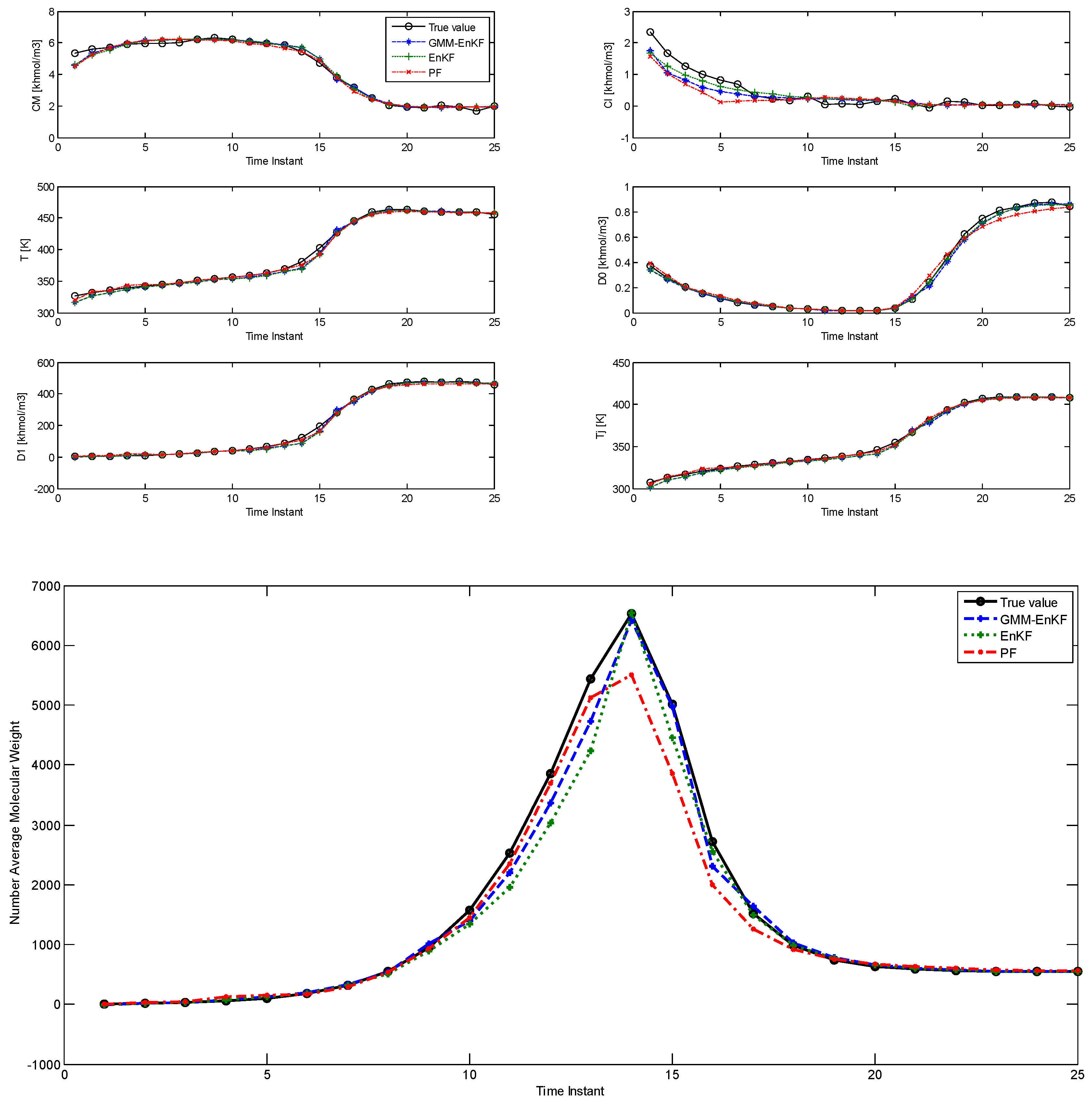
In this section, we present the results of applying the EnKF-GMM, EnKF, and PF algorithms on the PMMA process. To illustrate the performance of the estimators in cases where the states have multimodal distributions, bimodal process noise is applied to all the six states. The measurement noise is assumed to be Gaussian. The prior distribution of the state is also assumed to follow a GM distribution which contains two modes.
For Case Study 1, the true initial values of the states are:
The dynamics of the simulation describe how the system relaxes to a steady state from this initial condition. For the estimators, the initial particles are drawn from the prior distribution. The tuning parameters for the prior distribution are its mean and covariance. In the first case, a prior distribution with a small amount of bimodal process noise is tested for the three algorithms. The means of the two Gaussian modes of the prior distribution are:
The covariances of the modes of the prior distribution are:
The tuning parameters of the initial distribution indicate a state distribution with insignificant bimodality. The purpose of this simulation is to demonstrate the estimation performance of the three algorithms in the scenario where the state distribution shows insignificant multimodality.
The comparison of estimation results using the EnKF-GMM, EnKF, and PF is shown in Figure 1, with time steps on the x-axis (each time step is 0.3 h = 18 min). Table 2 shows the root mean squared error (RMSE) over the 25 time steps of the simulation for the six states and the NAMW for the three algorithms. In this case, the estimation results from Figure 1 and Table 2 show that the three algorithms have similar performance in estimation of the six states. However, the EnKF-GMM has the best performance in the estimation of the NAMW. In addition, the converged variance of the estimates of the states, obtained from the estimated covariance matrix with the EnKF-GMM, are [10−4, 10−4, 1.2 × 10⁻⁴, 10−5, 2 × 10⁻⁴, 4 × 10⁻⁴], respectively, confirming the significance of the estimates. The PF performs better than the EnKF only for some states. Increasing the number of particles for each of the algorithms to 200 (results not shown) improves the performance of the PF slightly, but the same conclusions hold.

Figure 1.
Comparison of the estimation performance of the ensemble Kalman filter (EnKF)-Gaussian mixture model (GMM), EnKF, and particle filter (PF) for the polymethyl methacrylate (PMMA) process with multimodal process noise (Case Study 1).
Table 2.
RMSE of the Gaussian mixture model based ensemble Kalman filter (EnKF-GMM), ensemble Kalman filter (EnKF), and particle filter (PF) for the polymethyl methacrylate (PMMA) process with multimodal process noise (Case Study 1).
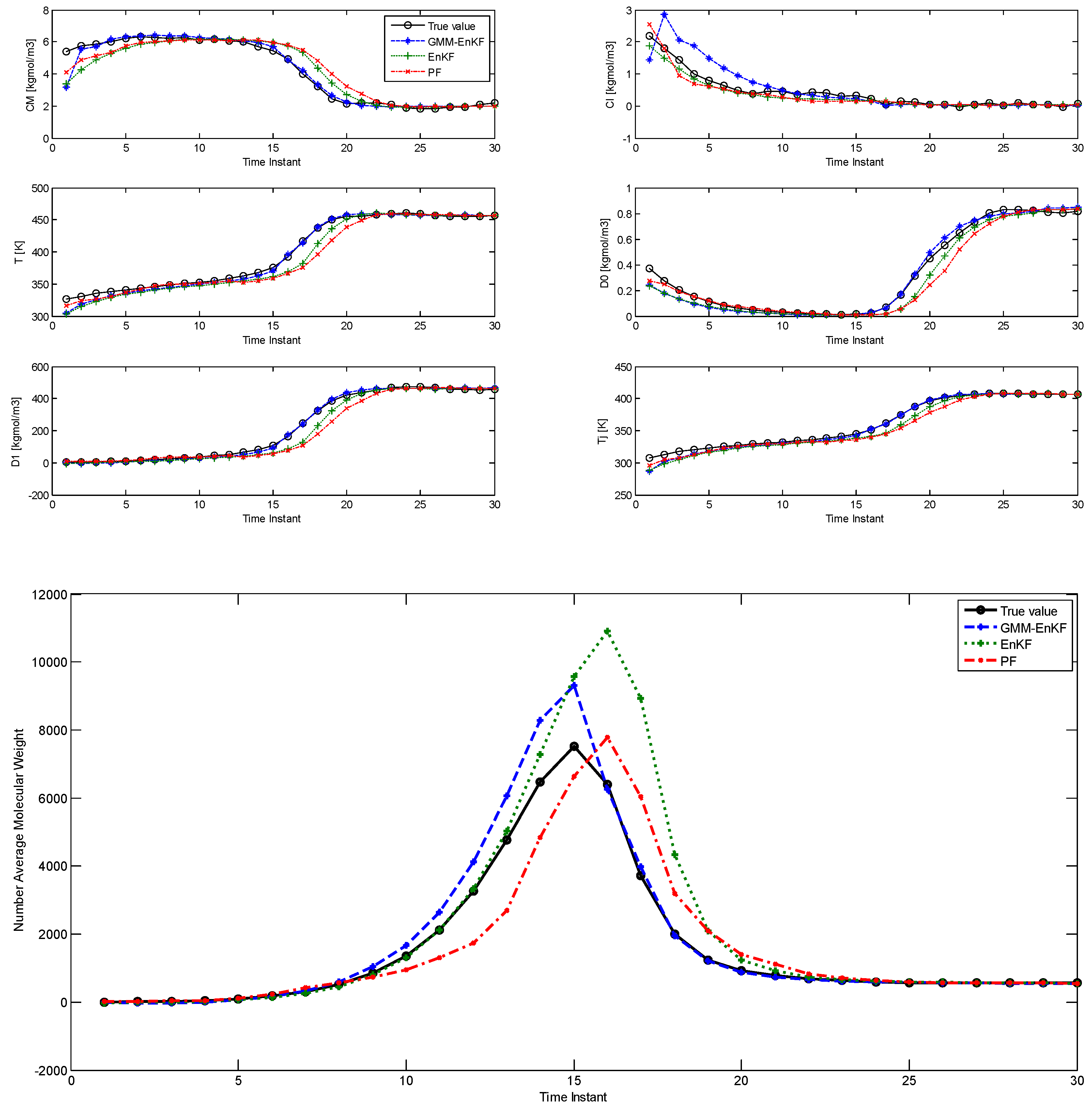
In Case Study 2, the multimodal features of the prior distribution are made more significant compared with the first case. The parameters of the prior distribution given below indicate that both modes lie far away from the true value, which also means that the initial condition mismatch is much larger. The true initial values of the states remain the same as the first case, and the process noise and measurement noise applied to the plant remain unchanged as well. The modified prior distribution is specified by:
In this case, the parameters of the prior distribution indicate that both of the modes lie near the tail of the likelihood function. The initial particles not only show significant multimodality, but also some degree of model-plant mismatch. The comparison of estimation using the EnKF-GMM, EnKF, and PF is shown in Figure 2 and the RMSE is shown in Table 3, and it is clear that the EnKF-GMM outperforms the other two estimators. As expected, the performance of the EnKF has worsened in this case because its Gaussian assumption on the prior and posterior distributions is violated in a significant manner. The PF does not show good performance either, and it is outperformed by the EnKF in the estimation of the NAMW. This is because the PF lacks robustness to plant-model mismatch [14], which is present in this case. Increasing the number of particles for all the estimators does not change these conclusions.

Figure 2.
Comparison of the estimation performance of the EnKF-GMM, EnKF, and PF for the PMMA process with more significant multimodal process noise (Case Study 2).
Table 3.
RMSE of the EnKF-GMM, EnKF, and PF for the PMMA process with more significant multimodal process noise (Case Study 2).
Figure 3 shows the evolution of the multimodal posterior distribution of the one of the states (the monomer concentration) at time steps 1, 3, 4, and 9. Table 4 lists the corresponding estimation errors of the three algorithms at those time steps with respect to the true value of . Figure 4 shows the evolution of the posterior distribution of another state (the jacket temperature) at time steps 2, 6, 9, and 10, and Table 5 shows the corresponding estimation errors of the three algorithms. These distributions are bimodal, and this clearly shows that the EnKF-GMM outperforms the other estimators in the presence of multimodal distributions.
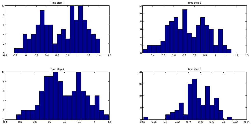
Figure 3.
Evolution of the multimodal posterior distributions of at time steps 1, 2, 4, and 9 (Case Study 2).
Table 4.
Comparison of the estimation errors of the EnKF-GMM, EnKF, and PF for at time steps 1, 3, 4, and 9 (in ) (Case Study 2).
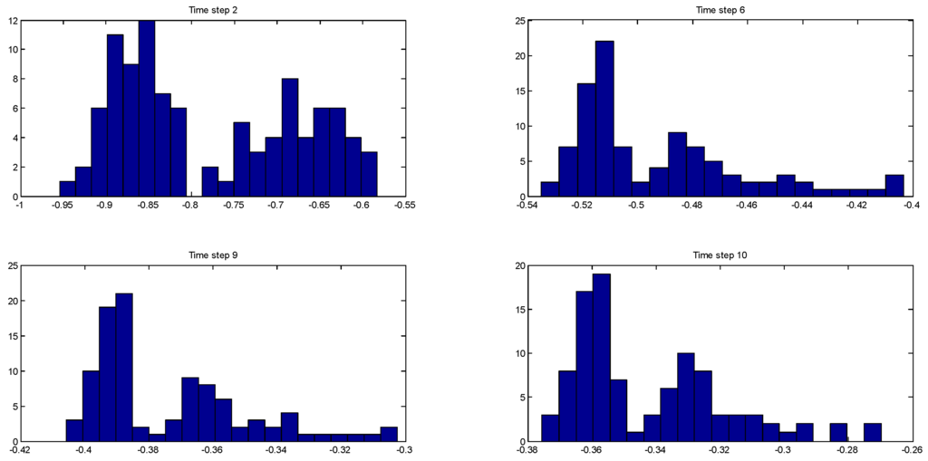
Figure 4.
Evolution of the multimodal posterior distributions of at time steps 2, 6, 9, and 10 (Case Study 2).
Table 5.
Comparison of the estimation errors of the EnKF-GMM, EnKF, and PF for at time steps 2, 6, 9, and 10 (in ) (Case Study 2).
3.3. Comparison of State and Parameter Estimation with the EnKF-GMM, EnKF and PF (Case Studies 3 and 4)
We consider the effects of parametric uncertainty in this section. The uncertain parameter chosen for these studies is , which is the activation energy associated with the reaction rate parameter . We choose as the uncertain parameter because (based on dimensionless sensitivity analysis) the NAMW is highly sensitive to the values of this parameter. We consider state estimation and joint state and parameter estimation in this section.
3.3.1. State Estimation with Uncertain Parameter (Case Study 3)
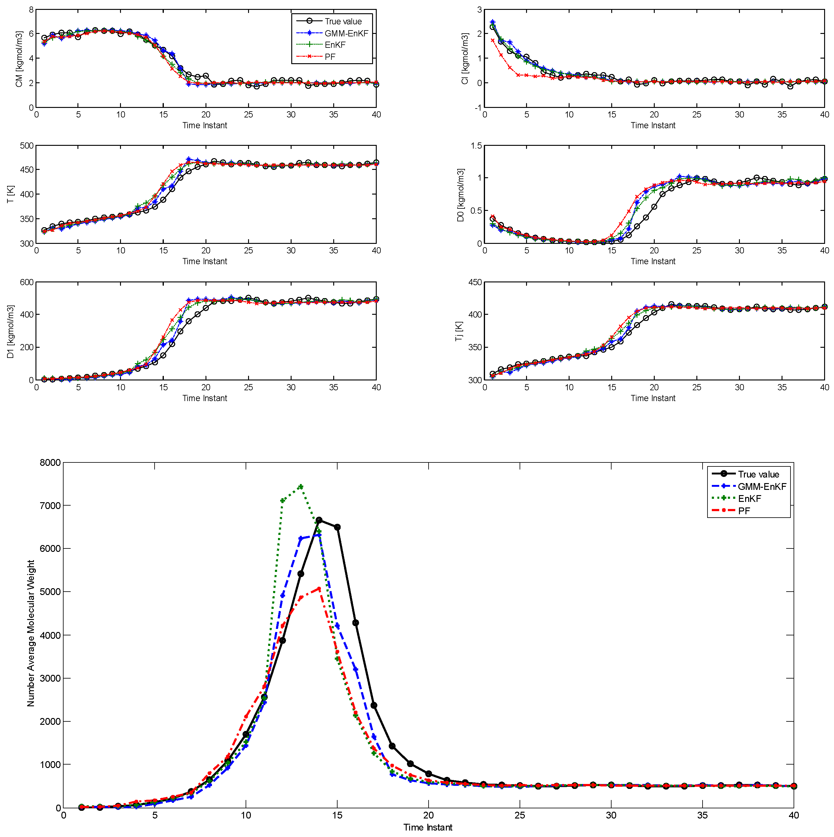
In this sub-section, while is an uncertain parameter and noise is added to its value at each time step in the simulation, the parameter is not estimated. The nominal value of is set to be , and bimodal Gaussian noise with means of the modes , and covariances , is added to it. In addition, process and measurement noise with the same distributions as in the second case in Section 3.2 are included. Figure 5 shows the comparison of the estimation results using the three algorithms over 40 time steps, and Table 6 shows the corresponding RMSE. In this case, the EnKF-GMM shows a small improvement in state estimation performance over the other estimators, especially in the estimation of the NAMW.
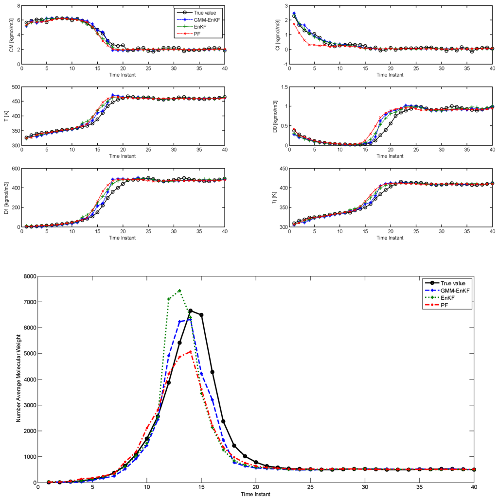
Figure 5.
Comparison of state estimation with the EnKF-GMM, EnKF, and PF for the PMMA process with uncertain parameter (Case Study 3).
Table 6.
RMSE of the EnKF-GMM, EnKF, and PF for state estimation in the case with uncertain parameter (Case Study 3).
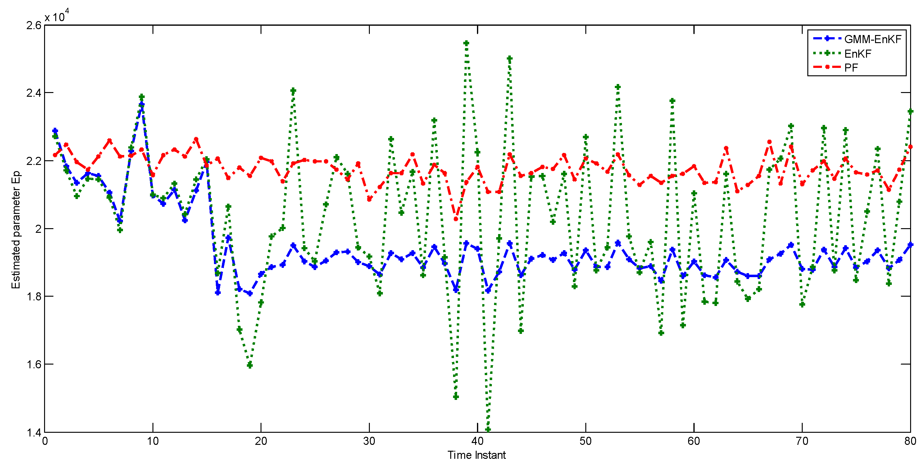
3.3.2. State and Parameter Estimation with Uncertain Parameter (Case Study 4)
Next, we compare the performance of the estimators for joint state and parameter estimation. Once again, is the uncertain parameter and its nominal value is kept the same as in Case Study 3. The parameter is treated as an augmented state for estimation. The prior distribution for has the following characteristics: means of , for its two modes, and covariances of , . Bimodal noise is added to each particle of the parameter, with means , and covariances , . Except for the exclusion of process noise, the properties of the simulation are kept the same as in Case Study 3. Figure 6 shows the performance of the estimators in state estimation, and Figure 7 shows their performance in estimating the parameter . While the performance of the EnKF in state estimation is comparable to that of the EnKF-GMM, the EnKF-GMM is clearly superior in parameter estimation. The PF has the worst performance among the estimators.
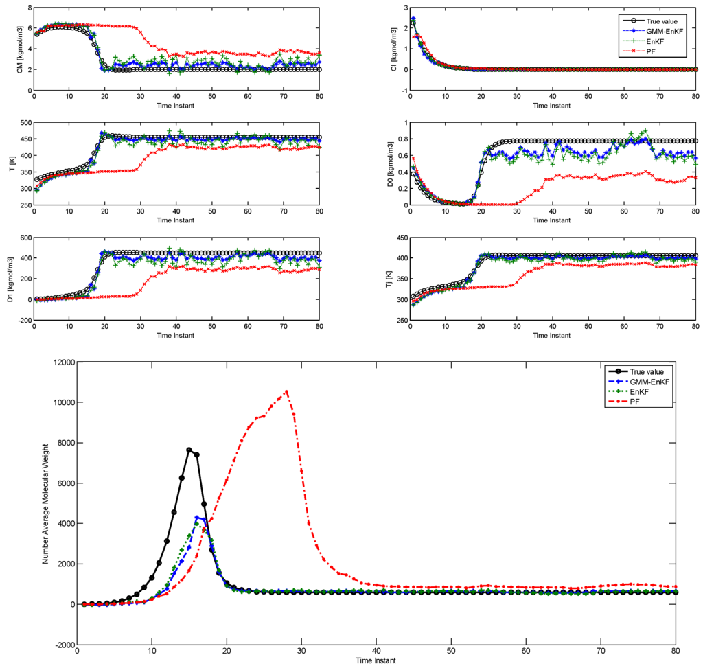
Figure 6.
Comparison of state estimation with the EnKF-GMM, EnKF, and PF for the PMMA process with uncertain parameters (Case Study 4).
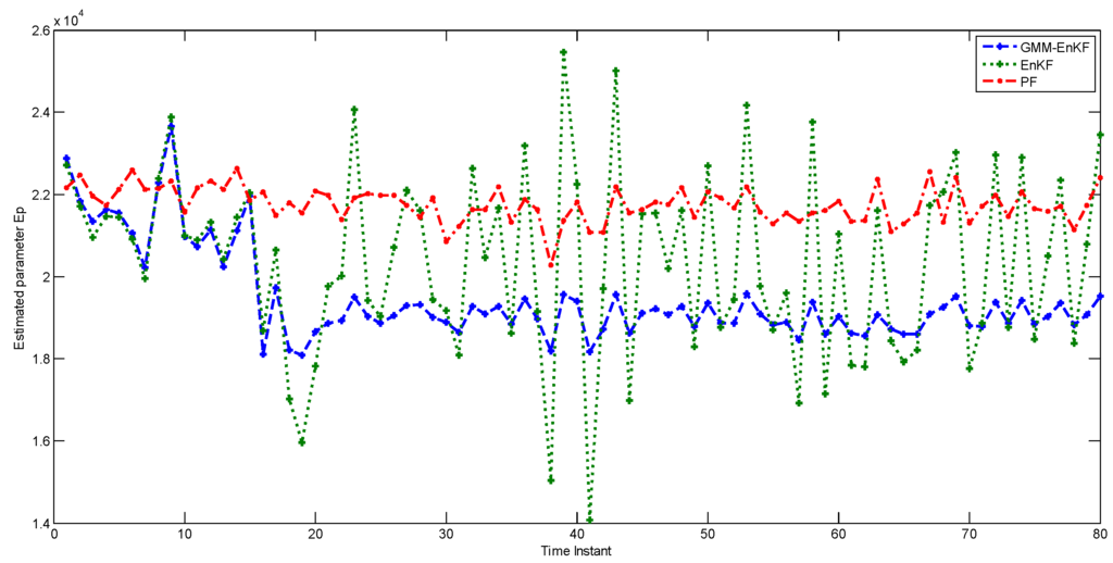
Figure 7.
Parameter estimation using the EnKF-GMM, EnKF, and PF (Case Study 4).
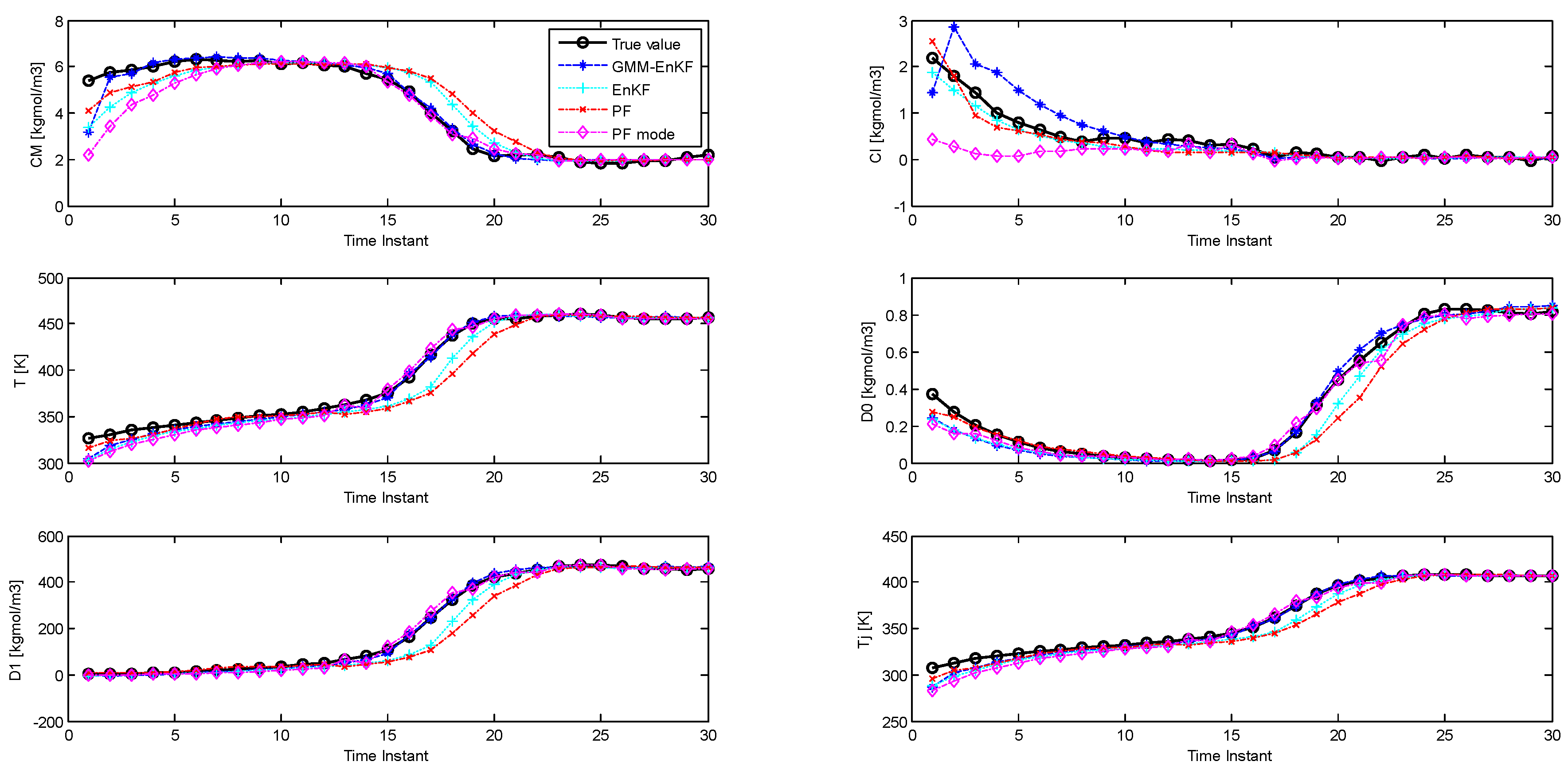
3.4. Alternate Point Estimates for the PF (Case Study 5)
In the PF, even though the full distribution is obtained, a point estimate for the states is usually obtained by choosing the expectation (mean) of the posterior particles. This is the method we have employed for the PF in the simulations described in the previous sections. However, if the distribution is multimodal, the mean may not necessarily represent the best point estimate, and the mode of the distribution (which is equivalent to the maximum a posteriori estimate) can provide a better estimate [14,31]. We investigate whether this approach can improve the performance of the PF, since we are considering cases where the distributions are multimodal. We apply k-means clustering on the posterior distribution of the particles to identify the modes and the maximum a posteriori estimate with the particle filter, and compare the estimation performance of this PF, called the PF-mode, with the other estimators. The parameters of the simulations are similar to the second case study. Figure 8 shows the performance of the estimators, and the RMSE is described in Table 7. The PF-mode clearly outperforms the PF and the EnKF; however, the EnKF-GMM has superior performance.

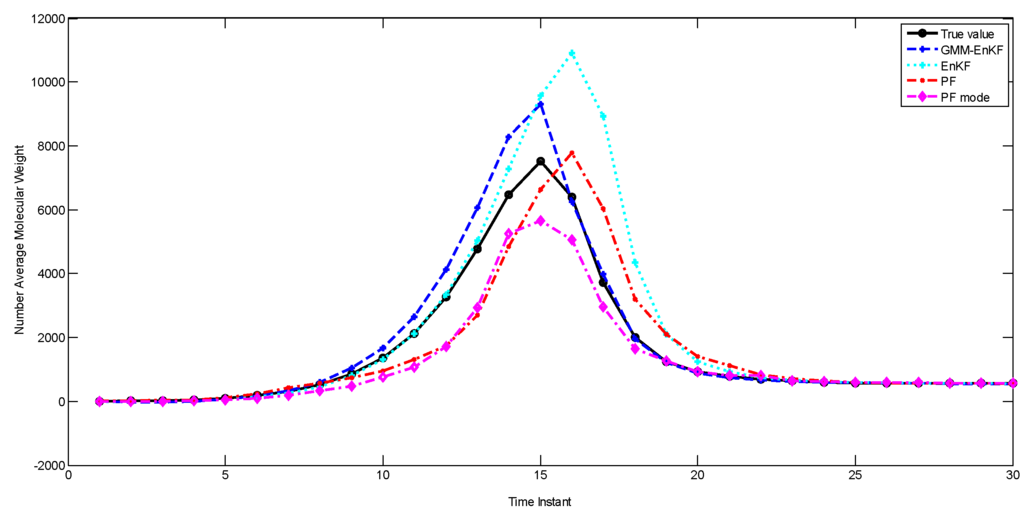
Figure 8.
Comparison of state estimation with the EnKF-GMM, EnKF, PF, and PF-mode (Case Study 5).
Table 7.
RMSE of the EnKF-GMM, EnKF, PF, and PF-mode for state estimation (Case Study 5).
The idea of the PF-mode is very similar to that of the EnKF-GMM. Both of them use clustering to extract modes from the posterior distribution and generate a point estimate based on the information in the modes. However, the EnKF-GMM outperforms the PF-mode because it is more robust to poor initial estimates and model-plant mismatch. Also, if the number of modes in the state distributions varies with time, perhaps even becoming unimodal at some times, using the mode as a point estimate is not necessarily superior to the mean. The EnKF-GMM combines the modes of the distribution in proportion based on the calculated weights to get a point estimate, and can adjust its estimation results in these cases by adjusting the weights of the modes.
4. Conclusions
We have proposed an estimator based on a Gaussian mixture model coupled with an ensemble Kalman filter (EnKF-GMM) that is capable of handling multimodal state distributions, and demonstrated its performance in simulations on a polymethyl methacrylate process. The EnKF-GMM clearly outperforms the particle filter (PF) and the EnKF in both state and parameter estimation with multimodal distributions. The EnKF is limited by the assumption of Gaussian distributions, and the particle filter’s performance is affected by its lack of robustness with respect to model-plant mismatch. A different choice for obtaining a point estimate with the particle filter, leading to a maximum a posteriori estimate, improves the performance of the PF, but the EnKF-GMM is still superior, indicating that it is the estimator of choice for systems with multimodal state distributions such as polymer processes.
Acknowledgments
The authors acknowledge financial support from the China Scholarship Council and the Natural Sciences and Engineering Research Council of Canada.
Author Contributions
All three authors conceived the work and participated in defining its scope. Ruoxia Li developed the algorithms and conducted the simulations described in the manuscript with inputs from Vinay Prasad and Biao Huang. Ruoxia Li wrote the initial drafts of the manuscript, and all authors contributed to the editing of the final manuscript and to the revisions.
Conflicts of Interest
The authors declare no conflict of interest.
References
- Wilson, D.; Agarwal, M.; Rippin, D. Experiences implementing the extended Kalman filter on an industrial batch reactor. Comput. Chem. Eng. 1998, 22, 1653–1672. [Google Scholar] [CrossRef]
- Prasad, V.; Schley, M.; Russo, L.P.; Bequette, W.B. Product property and production rate control of styrene polymerization. J. Process Control 2002, 12, 353–372. [Google Scholar] [CrossRef]
- Jo, J.; Bankoff, S. Digital monitoring and estimation of polymerization reactor. AIChE J. 1976, 22, 361–368. [Google Scholar] [CrossRef]
- Kozub, D.; MacGregor, J. State estimation for semi-batch polymerization reactors. Chem. Eng. Sci. 1992, 47, 1047–1062. [Google Scholar] [CrossRef]
- McAuley, K.; MacGregor, J. On-line inference of polymer properties in an industrial polymer properties in an industrial polyethylene reactor. AIChE J. 1991, 37, 825–835. [Google Scholar] [CrossRef]
- McAuley, K.; MacGregor, J. Nonlinear product property control in industrial gas-phase polyethylene reactors. AIChE J. 1993, 39, 855–866. [Google Scholar] [CrossRef]
- Sriniwas, G.; Arkun, Y.; Schork, F. Estimation and control of an alpha-olefin polymerization reactor. J. Process Control 1994, 5, 303–313. [Google Scholar] [CrossRef]
- Gopalakrishnan, A.; Kaisare, N.S.; Narasimhan, S. Incorporating delayed and infrequent measurements in extended Kalman filter based nonlinear state estimation. J. Process Control 2011, 21, 119–129. [Google Scholar] [CrossRef]
- Evensen, G. Sequential data assimilation with a nonlinear quasi-geostrophic model using Monte Carlo methods to forecast error statistics. J. Geophys. Res. 1994, 99, 10143–10162. [Google Scholar] [CrossRef]
- Julier, S.; Uhlmann, J.; Durrant-Whyte, H. A new approach for filtering nonlinear systems. In Proceedings of the American Control Conference, Seattle, WA, USA, 21–23 June 1995.
- Julier, S.; Uhlmann, J.; Durrant-Whyte, H. A new method for the nonlinear transformation of means and covariances in filters and estimators. IEEE Trans. Autom. Control 2000, 45, 477–482. [Google Scholar] [CrossRef]
- Arulampalam, S.; Maskell, S.; Gordon, N.; Clapp, T. A tutorial on particle filters for on-line non-linear/non-Gaussian Bayesian tracking. IEEE Trans. Autom. Control 2002, 30, 174–189. [Google Scholar]
- Chen, T.; Morris, J.; Martin, E. Particle filters for state and parameter estimation in batch processes. J. Process Control 2005, 15, 665–673. [Google Scholar] [CrossRef]
- Shenoy, A.V.; Prakash, J.; Prasad, V.; Shah, S.L.; McAuley, K.B. Practical issues in state estimation using particle filters: Case studies with polymer reactors. J. Process Control 2013, 23, 120–131. [Google Scholar] [CrossRef]
- Shao, X.; Huang, B.; Lee, J.M. Constrained Bayesian state estimation- A comparative study and a new particle filter based approach. J. Process Control 2010, 20, 143–157. [Google Scholar] [CrossRef]
- Crowley, T.J.; Meadows, E.S.; Kostoulas, E.; Doyle, F.D. Control of particle size distribution described by a population balance model of semibatch emulsion polymerization. J. Process Control 2000, 10, 419–432. [Google Scholar] [CrossRef]
- Kiparissides, C. Challenges in particulate polymerization reactor modeling and optimization: A population balance perspective. J. Process Control 2006, 16, 205–224. [Google Scholar] [CrossRef]
- Sajjadi, S.; Brooks, B.W. Unseeded semibatch emulsion polymerization of butyl acrylate: Bimodal particle size distribution. J. Polym. Sci. A Polym. Chem. 2000, 38, 528–545. [Google Scholar] [CrossRef]
- Doyle, F.J.; Soroush, M.; Cordeiro, C. Control of product quality in polymerization processes. In Proceedings of the Sixth International Conference on Chemical Process Control, Tucson, AZ, USA, 7–12 January 2001; AIChE Press: New York, NY, USA, 2002; pp. 290–306. [Google Scholar]
- Flores-Cerrillo, J.; MacGregor, J.F. Control of particle size distributions in emulsion semibatch polymerization using mid-course correction policies. Ind. Eng. Chem. Res. 2002, 41, 1805–1814. [Google Scholar] [CrossRef]
- Bengtsson, T.; Snyder, C.; Nychka, D. Toward a nonlinear ensemble filter for high-dimensional systems. J. Geophys. Res. 2003, 108, 35–45. [Google Scholar] [CrossRef]
- Smith, K.W. Cluster ensemble Kalman filter. Tellus 2007, 59A, 749–757. [Google Scholar] [CrossRef]
- Dovera, L.; Della Rossa, E. Multimodal ensemble Kalman filtering using Gaussian mixture models. Comput. Geosci. 2011, 15, 307–323. [Google Scholar] [CrossRef]
- Dempster, A.P.; Laird, N.M.; Rubin, D.B. Maximum likelihood from incomplete data via the EM algorithm. J. R. Stat. Soc. B 1977, 39, 1–38. [Google Scholar]
- Ormoneit, D.; Tresp, V. Improved Gaussian mixture density estimates using Bayesian penalty terms and network averaging. In Advances in Neural Information Processing Systems 8; Touretzky, D.S., Tesauro, G., Leen, T.K., Eds.; MIT Press: Cambridge, MA, USA, 1996; pp. 542–548. [Google Scholar]
- Ueda, N.; Nakano, R.; Ghahramani, Z.; Hinton, G.E. SMEM algorithm for mixture models. Neural Comput. 2000, 12, 2109–2128. [Google Scholar] [CrossRef] [PubMed]
- Schwarz, G. Estimating the dimension of a model. Ann. Stat. 1978, 6, 461–464. [Google Scholar] [CrossRef]
- Hu, X.; Xu, L. Investigation on several model selection criteria for determining the number of cluster. Neural Inf. Process.-Lett. Rev. 2004, 4, 1–10. [Google Scholar]
- Silva-Beard, A.; Flores-Tlacuahuac Silva, A. Effect of process design/operation on the steady-state operability of a methyl methacrylate polymerization reactor. Ind. Eng. Chem. Res. 1999, 38, 4790–4804. [Google Scholar] [CrossRef]
- Shenoy, A.V.; Prasad, V.; Shah, S.L. Comparison of unconstrained nonlinear state estimation techniques on a MMA polymer reactor. In Proceedings of the 9th International Symposium on Dynamics and Control of Process Systems (DYCOPS 2010), Leuven, Belgium, 5–9 July 2010.
- Bavdekar, V.A.; Shah, S.L. Computing point estimates from a non-Gaussian posterior distribution using a probabilistic k-means clustering approach. J. Process Control 2014, 24, 487–497. [Google Scholar] [CrossRef]


© 2016 by the authors; licensee MDPI, Basel, Switzerland. This article is an open access article distributed under the terms and conditions of the Creative Commons by Attribution (CC-BY) license (http://creativecommons.org/licenses/by/4.0/).