Measurable Disturbances Compensation: Analysis and Tuning of Feedforward Techniques for Dead-Time Processes

Abstract

In this paper, measurable disturbance compensation techniques are analyzed, focusing the problem on the input-output and disturbance-output time delays. The feedforward compensation method is evaluated for the common structures that appear between the disturbance and process dynamics. Due to the presence of time delays, the study includes causality and instability phenomena that can arise when a classical approach for disturbance compensation is used. Different feedforward configurations are analyzed for two feedback control techniques, PID (Proportional-Integral-Derivative) and MPC (Model Predictive Control) that are widely used for industrial process-control applications. The specific tuning methodology for the analyzed process structure is used to obtain improved disturbance rejection performance regarding classical approaches. The evaluation of the introduced disturbance rejection schemes is performed through simulation, considering process constraints in order to highlight the advantages and drawbacks in common scenarios. The performance of the analyzed structure is expressed with different indexes that allow us direct comparisons. The obtained results show that the proper design and tuning of the feedforward action helps to significantly improve the overall control performance in process control tasks.

1. Introduction

The vast majority of industrial processes require a tailored control architecture to fulfill the system requirements. In such a scheme, the control system should keep the controlled variable as close as possible to its desired value acting against external phenomena (disturbances) that affect process variables. Therefore, disturbances should be considered in the control problem design [1]. Due to their origin, disturbances can be classified as measurable and unmeasurable. The measurable disturbances are an important issue that must be considered in control schemes, especially for process control [2]. A typical industrial process is formed by several subsystems that interact with each other and influence the control loops. Moreover, there are many systems, especially bioprocesses, where the control system has to compensate for the external disturbances [3,4]. In industrial processes, the basic control structure consists of a feedback controller, since it is capable of providing reference tracking, while reducing the influence of plant-model mismatch and compensating for process disturbances [1,5]. It is usual that the control system only focuses on one of the listed problems, providing weak performance for the other issues [6]. The feedback controller can be implemented using numerous techniques and approaches; however, to improve the rejection of measurable disturbances, a feedforward scheme is usually introduced.

Feedforward from measurable disturbances was first used for drum-level control of tanks connected in series in 1925 [7]. Many of the other early applications were related to distillation columns’ control [8,9]. Nowadays, feedforward control is widely used as a complement to feedback to improve measurable disturbance compensation. In fact, this mechanism is implemented in most distributed control systems [1].

The ideal feedforward controller is computed as the quotient between the disturbance and the plant dynamics. However, this compensation is seldom realizable, e.g., a dead time may not be inverted. This drawback moved some authors to develop more sophisticated tuning rules during the past few decades. In [8], an open-loop design procedure for lead-lag feedforward filters was proposed. First, the static gain of the filter is obtained from pure static models. After that, the time constants are computed to reduce the integral error of the open-loop response without taking into account the effect of the feedback controller. Similar open-loop design strategies were also proposed by [7,10].

Successive works dealt with the drawback of not taking into account the feedback controller at the design stage. In [11], an additional feedforward control signal is also added to the feedback control error for decoupling purposes. In contrast, a least-squares procedure was introduced in [12] to obtain the parameters of the feedforward controller that minimize the norm of the disturbance residual output for a given feedback controller. Recently, robust feedforward control was also introduced. The interested reader is referred to [13,14] and [15,16] for the standard and internal model control approach, respectively, and to [17] for a quantitative feedback theory approach.

The so far commented design strategies rely on an optimization procedure to obtain the feedforward controller parameters. Nevertheless, as occurs with PID (Proportional-Integral-Derivative) control, most industrial controllers are implemented within a fixed structure [1], thus leading to a need for analytical tuning rules to deal with typically low-order processes. Portable simple tuning rules for lead-lag feedforward filters were introduced in [2,6,18] assuming that the plant dynamics are modeled with first-order plus dead time systems and considering step-like disturbances.

In industrial practice, PID controllers are widely used. This is due to their efficacy, relatively low complexity and numerous tuning methods [1]. In such a scheme, the feedback control loop is extended with classical feedforward to provide an anticipated action to provide the measurable disturbance compensation. This classical scheme can provide significant improvements in the overall control performance. However, this is possible only in very limited situations, since the feedforward compensator must result in an implementable structure. When a feedforward compensator results in a non-realizable structure, a special tuning procedure is required to take full advantage of this technique. This is especially visible in processes that are characterized by input-output and disturbance-output time delays. As previously mentioned, the feedforward tuning methodology attracts the attention of many researches, since important advantages can be obtained when the proper set up of feedforward action is used. In this work, the tuning guidelines provided in [14,18,19] are used, since they introduce a methodology that significantly improves the feedforward control performance.

On the other hand, the MPC (Model Predictive Control) approach is frequently used in process control, since it provides a unified solution for feedback and feedforward control, where most of the problems discussed above are solved intrinsically thanks to the form of the control approach. Moreover, the MPC techniques can consider many process constraints in an intrinsic way, since the control signal is computed through an optimization procedure. All of these features and possibilities to deal with multivariable systems makes MPC a powerful tool in industrial applications. From the disturbance compensation point of view, the most important advantages of MPC controllers are related to the incorporation of future disturbance information [20,21]. The MPC feedback and feedforward co-design procedure results in a tradeoff, where the controller tuning procedure is carried out taking into account the most important aspects. There exist several MPC formulations that can be used for disturbance compensation analysis providing the specific methodology in accordance with the analyzed features [17,22,23]. In [3,22,24], it was shown that the optimal MPC controller setup for disturbance attenuation results in high bandwidths in the feedback loop, and it is necessary to compensate this issue. Considering the aforementioned feature of the MPC feedforward compensator, in this work, we use the modified GPC (Generalized Predictive Control) scheme and tuning provided in [3]. Such a configuration provides a two-degree-of-freedom control scheme within the Filtered Smith Predictor (FSP)-based GPC [25], that improves the robustness capabilities of the resulting controller.

Taking into account the importance of the disturbance compensation problem and previous aspects, in this work, we focus on the processes, the dynamics of which involves the time delays. The analyzed configurations are focused on control problems related to process input-output and disturbance-output time delays. It is well known that time delays are a natural part of numerous processes. From the classical feedforward approach point of view, the presence of time delays may lead to a sluggish response, non-implementable structures and even result in unstable control. The typical solution for such systems is able to compensate the disturbance in an ineffective way (usually, only the invertible part is implemented). Despite this, the feedforward control schemes for dead time processes have not attracted much attention [26]. For this reason, in this work, the feedforward control problem for those processes is analyzed, and as a result, the control problem is reduced to a few configurations that can arise for such systems. Once the possible configurations are isolated, the feedforward compensators are evaluated for control schemes where PID and MPC approaches are used as feedback controllers. To this end, improved tuning methods are used for each approach. Several simulations are provided to highlight the main features, and a comparison using some performance indexes is performed [27].

The paper is organized as follows. The feedforward control problem is presented in Section 2, where a traditional feedback plus feedforward control loop and implicit disturbance compensation mechanisms of GPC are shown. Section 3 is devoted to explain the tuning rules for each approach considering different process configurations. Simulation examples to illustrate the responses of PID plus feedforward and the implicit GPC compensator are shown in Section 4. Additionally, several control performance indexes are computed for different process configurations and compared in this section. Finally, the paper ends with some conclusions on the analyzed structures [23].

2. Problem Statement

As mentioned previously, the feedforward compensation technique is not a new approach and is widely used in industrial applications (the feedforward completion technique is summarized in Appendix A). In this work, the the analysis of process disturbance is focused on the systems where the involved dynamics contains time delays, which make the classical feedforward approach less effective. For this reason, the two process transfer functions are modeled as first-order systems with time delay (see Appendix A for more details), i.e.,

$$P_u\left(s\right)=\frac{K_u}{1+s{T}_u}{e}^{-s{L}_u},P_v\left(s\right)=\frac{K_v}{1+s{T}_v}{e}^{-s{L}_v}$$

(1)

There are, of course, processes that are not well described by these simple transfer functions; but, for process control applications, this structure is mostly good enough, and it has become the standard model in process control applications.

From the feedforward control structure point of view, the previous assumption leads to three cases that can be formed considering the difference between input-output and disturbance-output time delays $\rho =L_u-L_v$:

$$\begin{array}{ccc}\hfill \rho <0,& \rho =0,& \rho >0,\hfill \\ & & \end{array}$$

These cases determine the basic configurations of the feedforward compensator that should be considered in the design method. For the first two cases, $\rho <0$ and $\rho =0$, feedforward compensators are implementable. The last case, $\rho >0$, represents the situation where the classical feedforward compensator is not realizable. Therefore, detailed analysis of the aforementioned configurations is presented, considering feedback controllers. First, the feedforward plus PID feedback controller is analyzed, highlighting the most important features. Next, the GPC approach is deeply analyzed and contrasted with classical compensators.

2.1. Feedback Plus Feedforward Controllers

First, low-order feedback and feedforward controllers are used. We consider that the feedback controller is a PI or PID controller, such that:

$$C\left(s\right)=K\left(1+\frac{1}{s{T}_i}+s{T}_d\right)$$

(2)

where K is the proportional gain, $T_i$ is the integral time and $T_d$ is the derivative time ($T_d=0$ in the case of a PI controller). Note that this is a basic structure used for analysis and design. In the real implementation, features like filters, anti-windup and limitations must be added.

Moreover, we also assume that the feedforward compensator is a lead-lag filter with a dead time (note that more complex structures are seldom used [28]), such that:

$$C_{ff}\left(s\right)=K_{ff}\frac{1+s{B}_{ff}}{1+s{T}_{ff}}{e}^{-s{L}_{ff}},$$

(3)

being $K_{ff}$ the static gain, $-1/B_{ff}$ the zero, $-1/T_{ff}$ the pole and $L_{ff}$ the dead time. Note that perfect disturbance compensation is achieved for $K_{ff}=K_v/K_u$, $B_{ff}=T_u$, $T_{ff}=T_v$ and $L_{ff}=-\rho$. However, since a negative dead time may appear, further analysis is required.

Hereafter, it is assumed that the feedback controller Equation (2) is designed to fulfill some closed-loop specifications, being the feedforward controller Equation (3) the sole tunable component for the measurable disturbance compensation problem.

2.2. Extended GPC with Implicit Feedforward Compensator

In this section, the extended GPC with the implicit feedforward compensator is shown, since this approach is used for the analyzed processes with time delays. The classic GPC with the feedforward compensator is summarized in Appendix B. The analysis provided below is a straightforward continuation of this from Appendix B.

Notice that matrix $\mathbf{H}$ depends on the relative difference between the input-output time delay and disturbance-output time delay, ${\rho }_d=d-d_v$. This leads to three different structures for matrix $\mathbf{H}$ based on the sign of ${\rho }_d$:

$${\rho }_d<0{\rho }_d=0$$

$$\mathbf{H}=\left[\begin{array}{cccccc}0& 0& 0& 0& 0& 0\\ 0& 0& 0& 0& 0& 0\\ \cdots & \cdots & \cdots & \cdots & \cdots & \cdots \\ 0& 0& 0& 0& 0& 0\\ h_0& 0& 0& 0& 0& 0\\ ⋮& \ddots & 0& 0& 0& 0\\ h_{N+{\rho }_d-1}& \cdots & h_0& 0& 0& 0\end{array}\right]\begin{array}{c}\left\}{\rho }_d\begin{array}{c}\begin{array}{c}\end{array}\\ \begin{array}{c}\end{array}\\ \begin{array}{c}\end{array}\\ \begin{array}{c}\end{array}\end{array}\right.\\ \\ \\ \end{array}\mathbf{H}=\left[\begin{array}{cccccc}{h}_0& 0& 0& 0& 0& 0\\ h_1& \ddots & 0& 0& 0& 0\\ ⋮& \ddots & \ddots & 0& 0& 0\\ ⋮& ⋮& \ddots & h_0& 0& 0\\ ⋮& ⋮& ⋮& \ddots & \ddots & 0\\ h_{N-1}& h_{N-2}& \cdots & & h_1& h_0\end{array}\right]$$

$${\rho }_d>0$$

$$\mathbf{H}=\left[\begin{array}{cccccc}{h}_{{\rho }_d}& h_{{\rho }_d-1}& \cdots & h_0& 0& 0\\ h_{{\rho }_d+1}& h_{{\rho }_d}& \ddots & \ddots & \ddots & 0\\ ⋮& \ddots & \ddots & \ddots & \ddots & h_0\\ ⋮& \ddots & \ddots & \ddots & \ddots & h_1\\ ⋮& ⋮& ⋮& ⋮& \ddots & ⋮\\ h_{N+{\rho }_d-1}& h_{N+{\rho }_d-2}& \cdots & \cdots & h_{{\rho }_d-1}& h_{{\rho }_d}\end{array}\right]\begin{array}{c}\\ \\ \\ \left\}{\rho }_d\begin{array}{c}\begin{array}{c}\end{array}\\ \begin{array}{c}\end{array}\\ \begin{array}{c}\end{array}\\ \begin{array}{c}\end{array}\end{array}\right.\end{array}$$

where $h_i$ are the coefficients of the $\mathbf{H}$ matrix obtained from the delay free disturbance response shifted in accordance to ${\rho }_d$. The previous prediction equation can be expressed as:

$$\widehat{\mathbf{y}}=\mathbf{Gu}+\mathbf{H}\mathbf{v}+\mathbf{f};\mathbf{f}={\mathbf{G}}_{\mathbf{p}}\Delta u(t-1)+{\mathbf{H}}_{\mathbf{p}}\Delta v\left(t\right)+\mathbf{S}y\left(t\right)$$

(4)

${\mathbf{G}}_{\mathbf{p}}$, ${\mathbf{H}}_{\mathbf{p}}$ and $\mathbf{S}$ are matrices of polynomials that are used to calculate the contribution to future process outputs of the past and present values of the process output, disturbance and control signal values (see [29] for more details). Then, Equation (4) becomes:

$$\widehat{\mathbf{y}}=\mathbf{Gu}+\mathbf{H}\mathbf{v}+{\mathbf{G}}_{\mathbf{p}}{u}_p+{\mathbf{H}}_{\mathbf{p}}{v}_p+\mathbf{S}{y}_p$$

(5)

where $u_p=\Delta u(t-1)$, $v_p=\Delta v\left(t\right)$ and $y_p=y\left(t\right)$ for simplicity.

Hence, the solution of the GPC controller is obtained minimizing J with respect to $\mathbf{u}$, which leads to:

$$\mathbf{u}={\mathbf{K}}^{-1}({\mathbf{G}}^{\top }\mathbf{w}-{\mathbf{G}}^{\top }\mathbf{S}{y}_p-{\mathbf{G}}^{\top }{\mathbf{G}}_{\mathbf{p}}{u}_p-{\mathbf{G}}^{\top }\mathbf{Hv}-{\mathbf{G}}^{\top }{\mathbf{H}}_{\mathbf{p}}{v}_p)$$

(6)

where $\mathbf{K}={\mathbf{Q}}_{\lambda }+{\mathbf{G}}^{\top }\mathbf{G}$.

Finally, according to the receding horizon strategy, only the first value of $\mathbf{u}$ is computed, $\Delta u\left(t\right)$. Hence, if $\mathbf{k}$ is the first row of matrix ${\mathbf{K}}^{-1}$, $\Delta u\left(t\right)$ is given by:

$$\Delta u\left(t\right)=\mathbf{k}{\mathbf{G}}^{\top }\mathbf{w}-\mathbf{k}{\mathbf{G}}^{\top }\mathbf{S}{y}_p-\mathbf{k}{\mathbf{G}}^{\top }{\mathbf{G}}_{\mathbf{p}}{u}_p-\mathbf{k}{\mathbf{G}}^{\top }\mathbf{Hv}-\mathbf{k}{\mathbf{G}}^{\top }{\mathbf{H}}_{\mathbf{p}}{v}_p$$

(7)

which is the well-known unconstrained control law for the GPC algorithm, including future knowledge of references and measurable disturbances. Remember that when constraints are taken into account, there is no explicit solution, and an optimization problem must be solved using a quadratic cost function with linear inequality and equality constraints [29].

The resulting unconstrained control law described by Equation (7) can be used to analyze the GPC algorithm from a block diagram point of view. Notice that the different terms in Equation (7) can be expressed as a set of different polynomials in the operator z that multiply the signals $w\left(t\right)$, $y\left(t\right)$, $\Delta u$ and $\Delta v\left(t\right)$, respectively. Thus, Equation (7) can be expressed as:

$$\Delta u\left(t\right)=m\left(z\right)w\left(t\right)+n\left(z\right)y\left(t\right)+l\left(z\right)\Delta u\left(t\right)+({\alpha }_f\left(z\right)+{\alpha }_p\left(z\right))\Delta v\left(t\right)$$

(8)

with:

$$m\left(z\right)=\mathbf{k}{\mathbf{G}}^{\top }{\mathbf{p}}_{\mathbf{z}}\left(z\right)=m_1{z}^{d+1}+m_2{z}^{d+2}+\cdots +m_N{z}^{d+N}$$

$${\mathbf{p}}_{\mathbf{z}}{\left(z\right)}^{\top }=[z^{d+1},z^{d+2},\cdots ,z^{d+N}]$$

$$n\left(z\right)=-\mathbf{k}{\mathbf{G}}^{\top }\mathbf{S}=n_1+n_2{z}^{-1}+\cdots +n_{na+1}{z}^{-na}$$

$$l\left(z\right)=-\mathbf{k}{\mathbf{G}}^{\top }{\mathbf{G}}_{\mathbf{p}}=l_1{z}^{-1}+l_2{z}^{-2}+\cdots +l_{nb+d}{z}^{-(nb+d)}$$

Moreover, ${\alpha }_p$ and ${\alpha }_f$ are, respectively, polynomials, including the coefficients of the past ($-\mathbf{k}{\mathbf{G}}^{\top }{\mathbf{H}}_{\mathbf{p}}$) and future ($-\mathbf{k}{\mathbf{G}}^{\top }\mathbf{H}$) values of the disturbance, which are calculated in different ways depending on the relation between the process input-output dead time, d, and the disturbance-output dead time, $d_v$. As a consequence, the ${\alpha }_{p,f}$ polynomials have the following forms:

a)

${\rho }_d<0$

$\begin{array}{c}{\alpha }_p\left(z\right)=\left\{\begin{array}{cc}{\alpha }_{p_1},\hfill & (nd+d_v)=1\hfill \\ {\alpha }_{p_1}+{\alpha }_{p_2}{z}^{-1}+\cdots +{\alpha }_{p_{(nd+d_v)}}{z}^{-(d_v+nd-1)},\hfill & (nd+d_v)>1\hfill \end{array}\right.\\ {\alpha }_f\left(z\right)={\alpha }_{f_1}{z}^1+{\alpha }_{f_1}{z}^2+\cdots +{\alpha }_{f_{N-(d_v-d+nd)}}{z}^{N-(d_v-d+nd)}\end{array}$

b)

${\rho }_d=0$

$\begin{array}{c}{\alpha }_{p\left(z\right)}=\left\{\begin{array}{cc}0,\hfill & (nd+d_v)=0\hfill \\ {\alpha }_{p_1},\hfill & (nd+d_v)=1\hfill \\ {\alpha }_{p_1}+{\alpha }_{p_2}{z}^{-1}+\cdots +{\alpha }_{p_{(nd+d_v)}}{z}^{-(d_v+nd-1)},\hfill & (nd+d_v)>1\hfill \end{array}\right.\\ {\alpha }_f\left(z\right)={\alpha }_{f_1}{z}^1+{\alpha }_{f_1}{z}^2+\cdots +{\alpha }_{f_N}{z}^N\end{array}$

c)

${\rho }_d>0$

$\begin{array}{c}{\alpha }_p\left(z\right)=\left\{\begin{array}{cc}0,\hfill & (nd+d_v)=0\hfill \\ {\alpha }_{p_1},\hfill & (nd+d_v)=1\hfill \\ {\alpha }_{p_1}+{\alpha }_{p_2}{z}^{-1}+\cdots +{\alpha }_{p_{(nd+d_v)}}{z}^{-(d_v+nd-1)},\hfill & (nd+d_v)>1\hfill \end{array}\right.\\ {\alpha }_f\left(z\right)={\alpha }_{f_1}{z}^{(d-d_v)}+{\alpha }_{f_1}{z}^{(d-d_v)+1}+\cdots +{\alpha }_{f_N}{z}^{(d-d_v)+N}\end{array}$

In the previous equations, $na$, $nb$ and $nd$ are the degrees of the polynomials A, B and D in Equation (A3), respectively. Notice that ${\alpha }_p$ and ${\alpha }_f$ polynomials can be grouped into $\alpha ={\alpha }_p+{\alpha }_f$, considering past and future values of the measurable disturbance. Thus, considering the previous polynomial representation, the GPC control law can be interpreted by the block diagram scheme presented in Figure 1. Then, from this figure, it can be observed that the resulting scheme has a typical feedback plus feedforward control, as shown in Figure A1. Hence, this interpretation allows one to clearly observe the internal feedforward structure of the GPC control algorithm and how the disturbance effect is managed in a similar way as a classical feedforward compensator. Furthermore, unlike a classical feedforward compensator, the prediction capabilities of the internal feedforward action can be also noticed through the use of future disturbance estimations, $\mathbf{v}$, by means of the polynomial ${\alpha }_f$.

3. Design Rules

3.1. Advanced PID Plus Feedforward Tuning Rules

In this section, simple tuning rules for lead-lag feedforward compensators that interact with PI or PID feedback controllers are described. For this purpose, a two-step design methodology is followed. First, the disturbance compensation speed is accelerated using the pole of the filter. Then, the gain of the feedforward compensator is adapted to reduce the interaction with the PI or PID controller.

3.1.1. Open-Loop Design

Let us consider that the dead time of the feedforward filter is set to obtain the fastest as possible disturbance compensation, i.e.,

$$L_{ff}=\text{max}(-\rho ,0),$$

(9)

and that the zero of the feedforward compensator is used to cancel the pole of $P_u\left(s\right)$, i.e.,

$$B_{ff}=T_u.$$

(10)

Then, the open-loop disturbance compensation is analyzed to tune the pole of the feedforward controller. As an initial assumption, let us consider that the feedforward static gain is defined as $K_{ff}=K_v/K_u$ and that the feedback controller is disconnected. Within this scenario, the open-loop transfer function for the disturbance compensation is given by:

$$\frac{y\left(s\right)}{v\left(s\right)}=P_v\left(s\right)-C_{ff}\left(s\right)P_u\left(s\right)=K_v\left(\frac{1}{1+s{T}_v}-\frac{1}{1+s{T}_{ff}}{e}^{-s\left(\rho +L_{ff}\right)}\right)e^{-s{L}_v}.$$

(11)

To clarify the effect of the pole of the compensator, some simulations are performed. Figure 2 shows the time-domain response of Equation (11) against a step change in v for different values of $T_{ff}$ with $K_v=L_v=\rho =0.5$. It can be seen that for smaller values of $T_{ff}$ that a faster disturbance compensation is obtained. However, if this parameter is chosen arbitrarily small, large overshoot error may appear in the final response [2,18].

Based on the time-domain response of Equation (11) against steps, analytical tuning rules are derived to design the pole of the compensator to meet one of the following requirements [2,18]: the removal of the overshoot; the minimization of the integral absolute error; and the minimization of the integral squared error. These rules were considered in the development of a more general tuning rule [18]:

$$T_{ff}=T_v-\frac{\rho +L_{ff}}{\alpha }$$

(12)

being $\alpha >(\rho +L_{ff})/T_v$ a free design parameter that determines the speed of the compensation. Furthermore, three proposals are given to choose this parameter as follows (see [18] for the derivation of the rules):

$$\alpha =\left\{\begin{array}{cc}{\displaystyle \frac{\rho }{2T_v\left(1-\sqrt{e^{-\frac{\rho }{T_v}}}\right)}}& \text{aggressive}\left(\text{R}1\right)\\ 1.7& \text{moderate}\left(\text{R}2\right)\\ 4& \text{conservative}\left(\text{R}3\right)\end{array}\right..$$

(13)

Note that in case that perfect compensation is realizable, i.e., $L_u\le L_v$, the pole of $C_{ff}\left(s\right)$ is the same as the pole of $P_v\left(s\right)$, since $\rho +L_{ff}=0$. In what follows, the assumption that the feedforward gain is designed as the inverted quotient ($K_{ff}=K_v/K_u$) is relaxed to improve the final disturbance compensation response.

3.1.2. Closed-Loop Adaption

After accelerating the disturbance compensation by adjusting the feedforward compensator pole, a modification of the feedforward static gain is proposed to improve the interaction between both controllers (feedback and feedforward). Note that, since both controllers try to attenuate the disturbance, usually larger overshoots than in the open-loop compensation may appear in the final response. To overcome this drawback, the static gain of the feedforward controller is reduced to take the control signal to the correct stationary level [2]:

$$K_{ff}=\frac{K_v}{K_u}-\frac{K}{T_i}IE,$$

(14)

being $IE$ an estimation of the integral error given by:

$$IE=K_v\left(\rho +L_{ff}+T_u-T_v+T_{ff}-B_{ff}\right).$$

(15)

Finally, by introducing the proposed values for $L_{ff}$, $B_{ff}$ and $T_{ff}$ into Equation (14), it is obtained that:

$$K_{ff}=\frac{K_v}{K_u}-\frac{K_{v}K}{T_i}\left(\rho +L_{ff}-\frac{\rho +L_{ff}}{\alpha }\right).$$

(16)

The interested reader is referred to [2] for a completely detailed analysis.

3.1.3. Tuning Guideline

The steps to tune the feedforward compensator are summarized next:

• Obtain the first-order plus dead-time transfer functions of the process $P_u\left(s\right)$ and $P_v\left(s\right)$ (see Equation (1)) following any of the well-known identifications, e.g., [1,30]. Note that previous references also provide simplification rules for higher order dynamics.
• Tune the PI or PID feedback controller Equation (2) at will to fulfill the given closed-loop specifications.
• Set $\rho =L_u-L_v$, and design $\alpha >(\rho +L_{ff})/T_v$ accordingly:

  $$\alpha =\left\{\begin{array}{cc}{\displaystyle \frac{\rho }{2T_v\left(1-\sqrt{e^{-\frac{\rho }{T_v}}}\right)}}& \text{aggressive}\\ 1.7& \text{moderate}\\ 4& \text{conservative}\end{array}\right.$$
• Tune the lead-lag feedforward controller Equation (3) using the proposed rules:

  $$\begin{array}{c}{L}_{ff}=\text{max}(-\rho ,0)\hfill \\ B_{ff}=T_u\hfill \\ T_{ff}=T_v-\left(\rho +L_{ff}\right){\alpha }^{-1}\hfill \\ K_{ff}=K_v\left(K_u^{-1}-K{T}_i^{-1}\left(\rho +L_{ff}\right)\left(1-{\alpha }^{-1}\right)\right)\hfill \end{array}$$
• If the control signal peak is not acceptable, increase $T_{ff}$ as needed.
• End of design.

3.2. Extended Design for GPC Implicit Feedforward Compensator

From Section 2.2, it was concluded that the GPC allows one to include implicit feedforward action in the predictive control law, but the disturbance effect cannot be perfectly canceled. The reason for this result can be understood analyzing the internal structure of the GPC and considering the influence of the λ parameter. The problem is that for values of $\lambda >0$, the internal feedforward action will never behave as a classical feedforward compensator, that is dividing the disturbance dynamics by the process one. This behavior can be only obtained with $\lambda =0$, as pointed out in [3].

This assertion can be corroborated by analyzing the GPC control law described by Equation (6). Consider that the system is in steady state and that the reference is set to zero ($w\left(j\right)=0,\text{for}j=t+d+1,\cdots ,t+d+N$, $y_p=y\left(t\right)=0$ and $u_p=\Delta u(t-1)=0$). Thus, Equation (6) becomes:

$$\mathbf{u}={({\mathbf{Q}}_{\lambda }+{\mathbf{G}}^{\top }\mathbf{G})}^{-1}(-{\mathbf{G}}^{\top }\mathbf{Hv}-{\mathbf{G}}^{\top }{\mathbf{H}}_{\mathbf{p}}{v}_p)$$

(17)

From this equation, it is possible to observe that the only way to obtain a typical feedforward compensator structure is by setting $\lambda =0$, and thus, ${\mathbf{Q}}_{\lambda }=0$. When this setting is used, it results:

$$\mathbf{u}=-{\mathbf{G}}^{-\mathbf{1}}\mathbf{Hv}-{\mathbf{G}}^{-\mathbf{1}}{\mathbf{H}}_{\mathbf{p}}{v}_p$$

(18)

where now the typical feedforward structure can be observed dividing the disturbance dynamics, $\mathbf{H}$ and ${\mathbf{H}}_{\mathbf{p}}$ for future and past disturbance values, respectively, by the process dynamics, $\mathbf{G}$, with the reverse sign.

Notice also that, when future disturbance values are not available, only the second term in Equation (18) is considered, and in this case, the GPC feedforward action is identical to that of a classical feedforward compensator, since only the actual value of the measurable disturbance is being considered, $v_p=\Delta v\left(t\right)$.

Thus, the proposed GPC with $\lambda =0$, which is focused on improving the disturbance rejection responses, is combined with a typical two-degree-of-freedom scheme, where a reference filter is included to achieve the desired set point tracking performance (and in some sense, to limit the control effort). Furthermore, the proposed control algorithm is implemented within the FSP-GPC framework to improve the robustness capabilities of the control system. These two ideas are briefly described in the following sections.

3.2.1. Reference Filter

The design of the reference filter has been performed in a classical way, that is by inverting the closed-loop dynamics of the feedback control loop and adding the desired dynamics for the set point tracking response. The closed-loop system dynamics can be obtained in the following way:

$$G_{cl}\left(z\right)=\frac{y\left(t\right)}{w\left(t\right)}=\frac{C\left(z\right)P_p\left(z\right)}{1+C\left(z\right)P_p\left(z\right)O\left(z\right)}=\frac{{\text{num}}_{cl}\left(z\right)}{{\text{den}}_{cl}\left(z\right)}$$

(19)

where $P_p\left(z\right)=\frac{B\left(z\right)}{A\left(z\right)}$, $C\left(z\right)=\frac{m\left(z\right)}{(1-l(z\left)\right)\Delta }$ and $O\left(z\right)=\frac{n\left(z\right)}{m\left(z\right)}$.

Thus, the reference filter, $F\left(z\right)$, can be designed in the following way:

$$F\left(z\right)=\frac{{\text{den}}_{cl}\left(z\right)}{{\text{num}}_{cl}\left(z\right)}\frac{f_{f0}}{{(z-a_f)}^n}$$

(20)

where $n\ge \text{degree}\left({\text{num}}_{cl}\left(z\right)\right)-\text{degree}\left({\text{den}}_{cl}\left(z\right)\right)$, $a_f$ is a filter tuning parameter and $f_{f0}$ is a coefficient to obtain a filter unitary gain [3,31].

3.2.2. FSP-GPC Approach

The FSP-GPC framework is a well-known control scheme, which helps to improve the GPC capabilities to deal with dead time processes and to face process uncertainties [25]. This scheme is a linear dead time compensator equivalent to the FSP, where the primary controller is tuned using an optimization procedure. This control scheme includes a new degree of freedom, the robustness filter, $F_r\left(z\right)$, which must be properly tuned for robustness purposes [25]. In the unconstrained case, the following two-step procedure can be used for tuning the controller, based on the ideas of dead time compensation control [25]:

• Compute the horizons and weighting factors in order to obtain the desired set point tracking performance for the nominal plant, such as described in the previous sections.
• Estimate the uncertainties of the plant, and tune the filter $F_r\left(z\right)$ in order to obtain robust stability and the highest bandwidth for the disturbance rejection performance.

To understand the effect of $F_r\left(z\right)$ on the closed-loop system, let us consider the relationship between the disturbance and the output:

$$\frac{Y\left(z\right)}{V\left(z\right)}=P\left(z\right)\left(1-\frac{C_{fsp}\left(z\right)F_r\left(z\right)P_n\left(z\right)z^{-d}}{1+C_{fsp}\left(z\right)P_n\left(z\right)}\right),$$

(21)

and the following robustness condition:

$$dP\left(\omega \right)=\frac{\mid 1+C_{fsp}\left(z\right)P_n\left(z\right)\mid }{\mid C_{fsp}\left(z\right)P_n\left(z\right)F_r\left(z\right)\mid }>\mid \delta P\left(z\right)\mid ,z=e^{j\omega }\forall \omega \in [0,\pi ].$$

(22)

where $\delta P\left(z\right)$ is the multiplicative modeling error, $P_n\left(z\right)$ is the nominal model without delay and $C_{fsp}\left(z\right)$ is the equivalent primary controller of the FSP-GPC [25].

From these equations, it is clear that if $F_r\left(z\right)$ is a low pass filter, the robustness can be improved. The condition for the steady-state step disturbance rejection of the system is that the same factor has a zero at $z=1$ (notice that for the nominal case and with $\lambda =0$, the measurable disturbances are completely removed by the implicit feedforward compensator of the GPC). This implies the following conditions:

$$\left\{\begin{array}{c}\hfill {\left.\left(F_r\left(z\right)-z^d\right)\right|}_{z=1}=0\\ \hfill {\left.\left(F_r\left(z\right)-z^d\right)\right|}_{z=z_o}=0\end{array}\right.$$

(23)

Therefore, as shown in previous conditions, the disturbance rejection properties of the closed-loop system only depend on $F_r\left(z\right)$ and d. Further information regarding the robustness filter can be found in [25].

4. Results and Discussion

This section presents the simulation results of the analyzed feedforward strategies for both approaches that consider PID and GPC algorithms. Firstly, the process configuration with the realizable feedforward compensator is introduced. This example is used to show the classical approach and to highlight the limitations of the GPC implicit feedforward action based on the classic scheme. Secondly, the non-realizable feedforward compensator is studied to analyze the advantages and drawbacks for the feedforward compensator design in PID and GPC approaches. Additionally, a third example is considered to test the studied techniques against process constraints. In this case, the process is set to result in a non-realizable compensator, and the control system is limited by the control signal saturation. Finally, several control system performance indexes are computed to show the individual properties of each configuration.

In all of the presented simulations, the PID and GPC controllers keep the same parameters, and only those released to the disturbance compensation are modified to obtain the desired performance. As previously mentioned, the analyzed process is represented by the first-order systems (see Equation (27)), which are used to setup the feedback controller. Consider that the PID feedback controller is designed according to the SIMCtuning rule [30], such that $K=0.5$ and $T_i=1$. Moreover, the GPC controller with implicit feedforward action was implemented with the following parameters: prediction and control horizons were set to $N=15$, $N_u=5$ and $\delta =1$, respectively. The reference filter value has been set to zero, since it has no influence over the analyzed implicit disturbance compensation mechanism. The GPC control scheme has been implemented with a sampling time $T_s=0.1$ seconds to obtain the discrete time polynomials $A\left(z^{-1}\right)$, $B\left(z^{-1}\right)$ and $D\left(z^{-1}\right)$ from the transfer functions $P_u\left(s\right)$ and $P_v\left(s\right)$.

To determine the control performance for each analyzed configuration, the following indexes have been considered:

$$IAE={\int }_0^{\infty }\left|e\left(t\right)\right|dt$$

(24)

$$IAC={\int }_0^{\infty }\left|u\left(t\right)\right|dt$$

(25)

$$CSE=\left|\right|\Delta u\left(t\right)\left|\right|$$

(26)

where $IAE$ represents the Integrated Absolute Error between reference and controlled variable, the $IAC$ refers to the Integrated Absolute Control signal and $CSE$ stands for the Control System Effort (computed as the normalized value of the discrete/discretized controls’ signal increments $\Delta u\left(t\right)$).

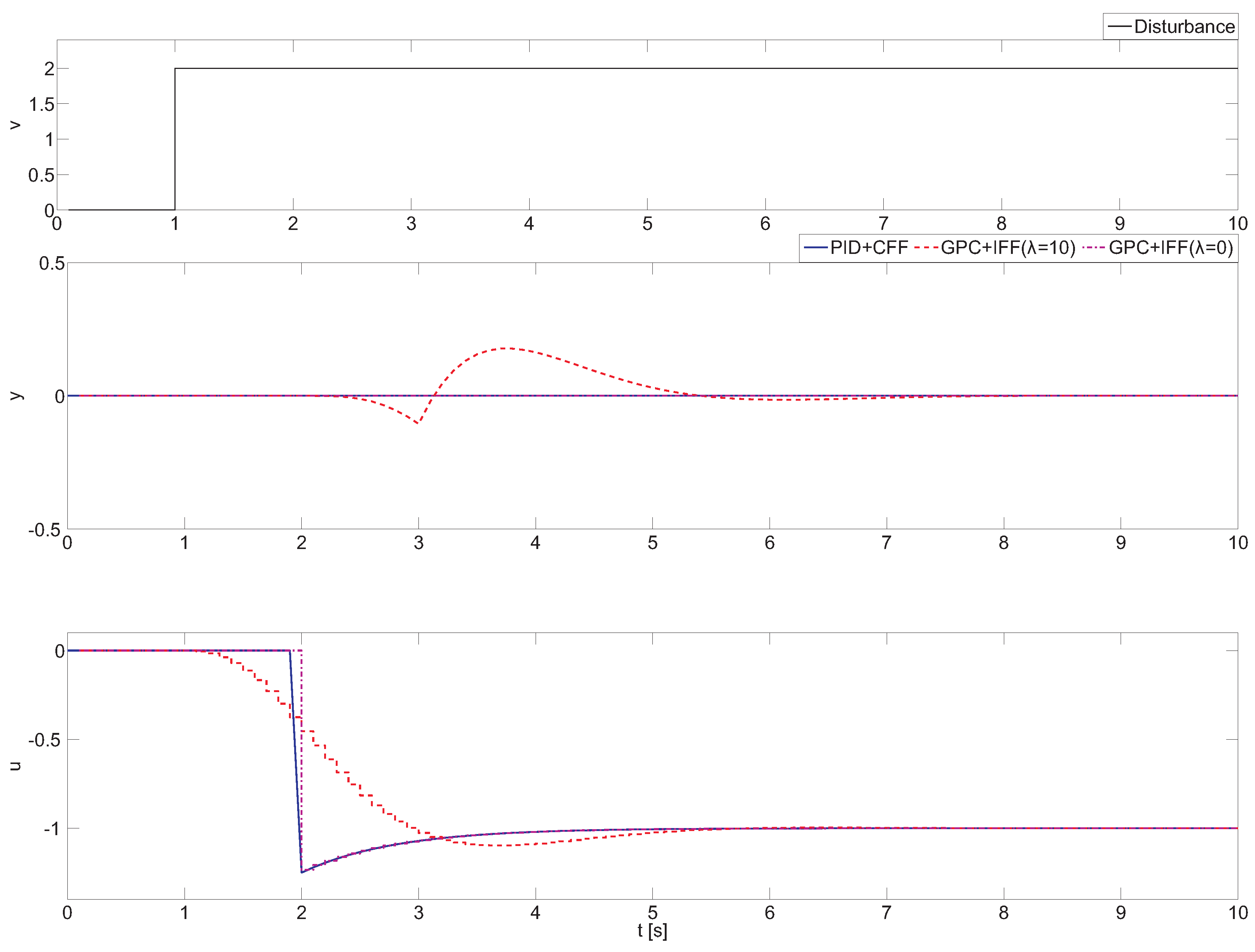
For the first example, the process transfer functions have been set up as follows:

$$\begin{array}{c}\hfill P_u\left(s\right)=\frac{1}{1+s}{e}^{-s},P_v\left(s\right)=\frac{0.5}{1+0.8s}{e}^{-s},\end{array}$$

(27)

In such a case, the resulting dead time difference $\rho <0$, and as a consequence, a classical feedforward compensator is realizable by dividing $P_u\left(s\right)$ and $P_v\left(s\right)$ with the reverse sign [2]. Moreover, the GPC simulations for this example have been performed using two different values for λ, $\lambda =10$ and $\lambda =0$, respectively. The obtained results are shown in Figure 3, where it can be observed that when a classical feedforward compensator is used (PID + CFF), a perfect cancellation is obtained.

The situation changes for the next analyzed configuration, the GPC with implicit feedforward and control weighing factor $\lambda =10$ (GPC + IFF(λ)). For this case, the implicit feedforward GPC controller starts to react in advance with respect to the classical feedforward controller thanks to the prediction capabilities of the GPC algorithm. However, the most important issue is that the GPC algorithm is not able to eliminate the disturbance effect. This result shows that the prediction capabilities of the GPC algorithm are not effective, and the GPC parameters must be properly tuned to reach a perfect disturbance effect cancellation (as was shown in Section 2.2). Furthermore, this study allows one to observe the influence of the λ design parameter in the disturbance rejection responses. However, this problem can be overcome by applying the previously introduced extended design for GPCs’ feedforward action and setting $\lambda =0$. It can be observed that GPC + IFF ($\lambda =0$) obtains perfect compensation, since the unweighted control signal is used. Based on this feature, significant improvements can be obtained also for non-realizable configurations, which are analyzed below.

The performance for the analyzed process configurations are summarized in

Table 1. Performance indexes for different configurations of PID (Proportional - Integral - Derivative) and GPC (Generalized Predictive Control) feedforward control schemes. $IAE$, Integrated Absolute Error; $IAC$, Integrated Absolute Control; $CSE$, Control System Effort.

	PID + CFF	GPC + IFF ($\mathbf{\lambda }\mathbf{=}\mathbf{10}$)	GPC + IFF ($\mathbf{\lambda }\mathbf{=}\mathbf{0}$)
$IAE$	0	0.276	0
$IAC$	8.31	13.13	13.29
$CSE$	0.15	0.12	0.14

. In accordance with the previously described results, the PID + CFF and GPC + IFF ($\lambda =0$) obtain perfect compensation ($IAE$ = 0). In the GPC case, more control effort is required to achieve disturbance attenuation ($IAC$ values). However, the PID + CFF scheme produces more aggressive changes in the control signal ($CSE$ = 0.12).

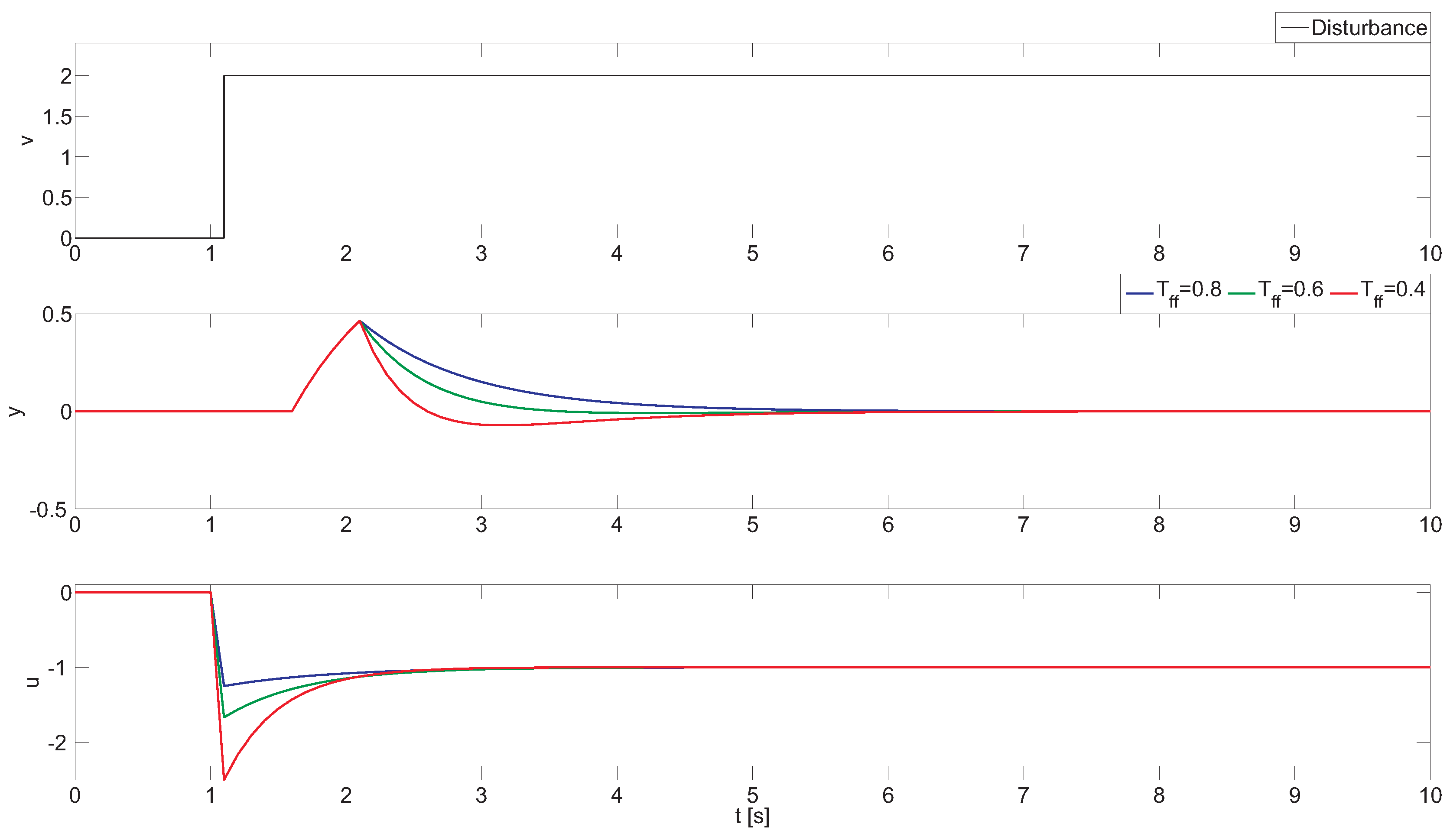
To prove the effectiveness of the proposed design strategies, let us consider that the process is given by the transfer functions:

$$\begin{array}{c}\hfill P_u\left(s\right)=\frac{1}{1+s}{e}^{-s},P_v\left(s\right)=\frac{0.5}{1+0.8s}{e}^{-0.5s},\end{array}$$

(28)

such that $\rho =0.5$. Thus, the ideal feedforward compensator cannot be formed due to a non-realizable delay inversion. Hereafter, PID plus feedforward and GPC with implicit feedforward controllers are designed according to the previously defined tuning rules. First, following the tuning guideline of Section 3.1.3, PID plus feedforward controllers are explored, and the following lead-lag feedforward filters are obtained:

$$C_{ff}\left(s\right)=\left\{\begin{array}{cc}{\displaystyle 0.50\frac{1+s}{1+0.80s}}& \text{invertible}\\ {\displaystyle 0.48\frac{1+s}{1+0.37s}}& \text{aggressive}\\ {\displaystyle 0.45\frac{1+s}{1+0.51s}}& \text{moderate}\\ {\displaystyle 0.41\frac{1+s}{1+0.67s}}& \text{conservative}\end{array}\right.$$

(29)

In the GPC approach, the implicit feedforward compensator has been implemented following the scheme shown in Section 3.2. Furthermore, $\beta =0.65$ for the robustness filter $F_r\left(z\right)$ was selected for all configurations. Additionally, two simulations have been performed to analyze the GPC compensator. The first one includes only past measured disturbances in control signal computations, and the second one considers additionally the future disturbance value in the prediction mechanism.

Figure 4 shows the control results for PID with invertible part (PID + CFF), aggressive tuning (PID + R1FF), moderate tuning (PID + R2FF) and conservative tuning (PID + R3FF). Moreover, two GPC configurations, GPC + IFF ($\lambda =10$) and including future disturbance information, GPC + IFF($\lambda =0$) + F, are shown. In such an example, all of the analyzed configurations are tested against a step change in v of a magnitude of two at $t=1$. Notice that for this example, the control system set point was set to one in $t=0.1$. It can bee seen that all provided configurations reach the reference, and the desired performance can be obtained by proper tuning of the feedback controller.

For this case, the resulting dynamics have a non-causal form, which means that future information is required in the resulting feedforward compensator structure. In the classic feedforward design (PID + CFF), only the causal part is implemented, and the non-causal part is omitted. This leads to obtaining a poor disturbance rejection response, as shown in Figure 4. The same problem appears for the GPC with implicit disturbance compensator and without future information GPC + IFF ($\lambda =10$), where the disturbance model is included within the predictive control structure, but only the past disturbance measures are used. In this case, the disturbance effect compensates much faster than in PID + CFF. This improvement is obtained at the expense of the aggressive change in the control signal (bottom plot in Figure 4). This issue can be partially overcome using different tuning rules for the PID + feedforward scheme that improves the classical approach in compensation performance and simultaneously preserves the control resources. This behavior can be observed for the (PID + R1FF), (PID + R2FF), (PID + R2FF)configurations, where the compromise between compensation performance and control effort can be achieved. This property can be very useful in industrial practice where aggressive changes in control signal should be avoided.

Nevertheless, none of the previous cases completely eliminate the effect of the measurable disturbance, since the future information is not considered for the non-causal part. Complete disturbance compensation can be obtained when the future information is considered in the GPC + IFF ($\lambda =0$) + F control scheme. It becomes possible to remove the influence of the disturbance thanks to the predictive capabilities of the control algorithm, as observed in Figure 4. However, in contrast to the previous configurations, future disturbance information is required, not always being available. In this configuration, the control signal is less aggressive, but also, the velocity of the disturbance response can be managed by means of the robust filter design, $F_r\left(z\right)$, and the β tuning parameter [3,25].

The corresponding performance indexes are summarized in

Table 2. Performance indexes for different configurations of PID and GPC feedforward control schemes.

	PID + CFF	PID + R1FF	PID + R2FF	PID + R3FF	GPC + IFF ($\mathbf{\lambda }\mathbf{=}\mathbf{10}$)	GPC + IFF ($\mathbf{\lambda }\mathbf{=}\mathbf{0}$) + F
$IAE$	0.39	0.24	0.22	0.28	0.10	0
$IAC$	5.79	5.88	5.89	5.99	6.26	5.75
$CSE$	0.09	0.21	0.13	0.09	0.82	0.33

. Notice that for this particular example, the indexes were computed between $t=9$ and $t=20$; this is due to the different transient response of feedback controllers originated from the setpoint change. It can be observed that GPC + IFF ($\lambda =0$) + F obtains $IAE=0$, providing perfect disturbance attenuation. Moreover, the $IAC$ index shows that the required control effort can be adjusted in PID + FF schemes. From the $CSE$ values, it can be observed that GPC-based compensators require more aggressive changes in the control signal, but also provide better disturbance attenuation.

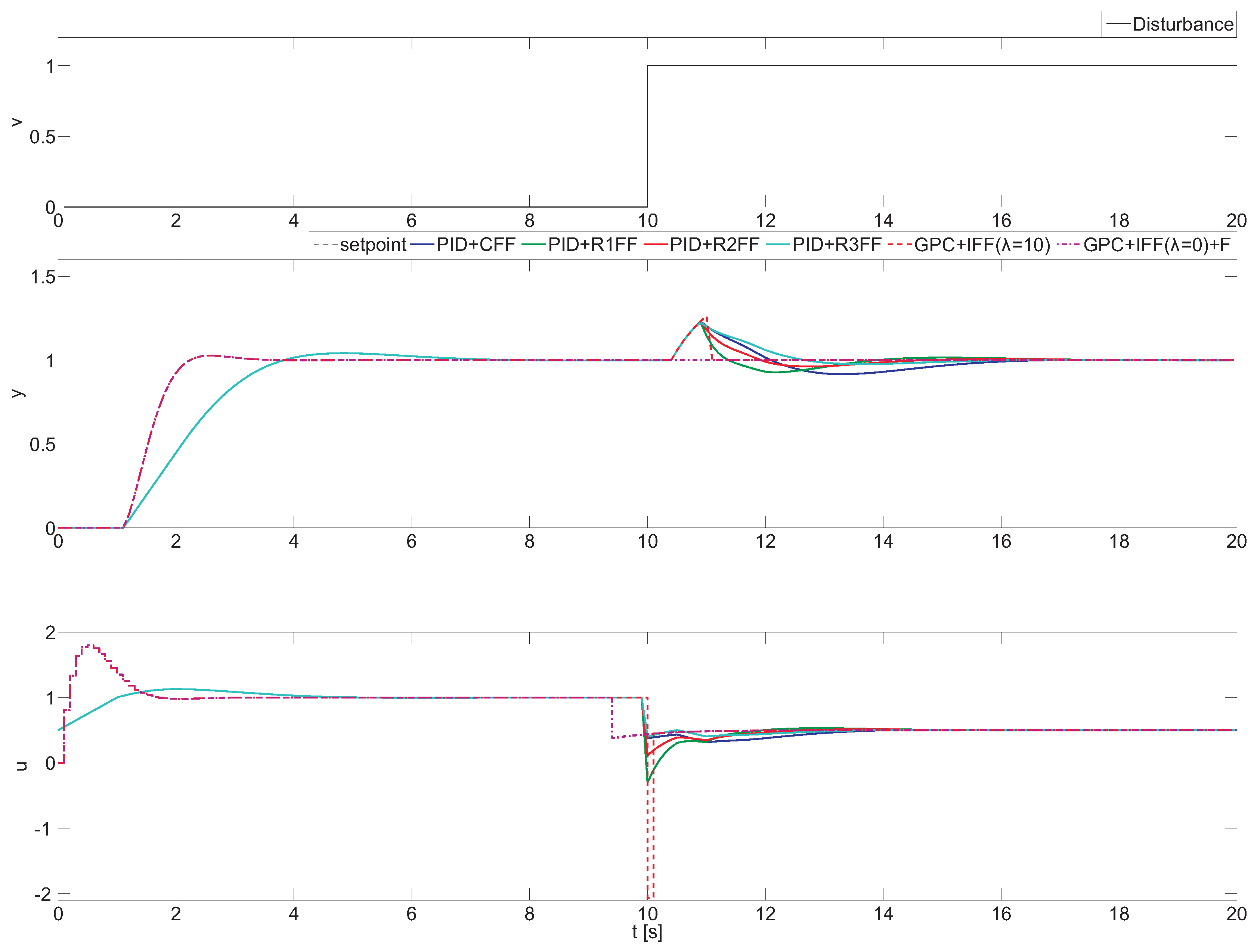
Furthermore, a last simulation is performed to demonstrate that the proposed tuning rules are also valid under the presence of input saturation. The tested configurations are the same as in the previous example and are evaluated against periodic squared disturbance. In the PID approaches, the process constraints are considered outside the controller structure; in the GPC-based schemes, the control signal limitations are taken into account using a constraint handling mechanism. The only difference is that now the robust filter is included in the control scheme, where $\beta =0.8$ has been selected. Figure 5 shows the simulation results for several consecutive steps in v assuming that $u\left(t\right)\in [-0.5,0.5]$.

In the first part of the simulation, the squared disturbance with an amplitude of $0.5$ is considered, and the disturbance effect is the same as in the previous example, since the required change in the control signal is possible. During this example, the GPC + IFF ($\lambda =10$) configuration obtains the worst compensation performance. This is mainly due to the effect of control signal weighting factor λ. This configuration has been selected consciously to show that a badly-tuned implicit GPC compensator could produce weak disturbance compensation. In the second part of the simulation, the amplitude of the disturbance signal is increased to one at the time instant $t=60$. Now, the control signals exceed the saturation limits, and differences are observed among the selected feedforward control configurations. The PID plus feedforward configurations keep all of the properties from the previous example and are able to reduce the disturbance effect taking into account the control effort. This can be observed in (PID + R1FF), (PID + R2FF) and (PID + R3FF), where the first one is more aggressive, and the last one requires a lower control effort. Notice how the GPC + IFF ($\lambda =0$) + F manages much better the process input constraints, reducing the disturbance effect and only having steady-state error when the system is saturated (in nonlinear mode). The reason is because the feedforward compensator is implicit in the GPC algorithm, and thus, the combined control signal from the feedback plus feedforward actions is considered in the optimization problem. Additionally, it can be observed that this configuration starts to compensate even before the disturbance effect appears on the process output. Due to this feature, significant improvements are obtained, and the controlled variable stays closer to the control system reference.

Table 3. Performance indexes for different configurations of PID and GPC feedforward control schemes.

	PID + CFF	PID + R1FF	PID + R2FF	PID + R3FF	GPC + IFF ($\mathbf{\lambda }\mathbf{=}\mathbf{10}$)	GPC + IFF ($\mathbf{\lambda }\mathbf{=}\mathbf{0}$) + F
$IAE$	7.15	4.62	5.50	6.72	10.61	3.76
$IAC$	47.36	47.85	47.38	46.89	45.31	43.98
$CSE$	0.97	1.02	0.98	0.95	1.54	1.55

summarizes the obtained values for all analyzed approaches. Analyzing the $IAE$ index, it can be observed that all new tuning rules (PID + R1FF, PID + R2FF, PID + R2FF) improve in performance the classical feedforward compensator that is formed only by the part of the dynamics that can be inverted. However, the GPC + IFF ($\lambda =0$) + F configuration achieves the smallest $IAE$ value, improving the best PID + FF configuration at about 20%. On the other hand, the GPC + IFF ($\lambda =10$) scheme obtains a worse performance due to the tuning issues previously mentioned. With the $IAC$, it can observed that almost all structures need similar control effort; this is mainly due to process constraints, since all tested configurations saturate the system. Only the GPC + IFF ($\lambda =0$) + F produces less variation in the control signal, reducing the average value around 7%. This is because of the future disturbance information that is considered in the prediction mechanism. Furthermore, due to the used FSP-GPC approach, the required control effort is also affected by the robustness filter setup, since there is an error between the nominal model and the process output due to saturation limits. The situation changes when the $CSE$ index is evaluated, since it takes into account the control effort in terms of changes in control signal increments. For this particular measure, a higher value represents that the feedforward controller produced a control signal with more aggressive changes. According to this index, both GPC-based approaches are more aggressive in comparison to the PID + FF configurations. Particularly, the $CSE$ index for the PID + R3FF scheme is about 40% lower when compared to the GPC + IFF($\lambda =0$) + F configuration. This outcome clearly indicates that the PID + R3FF compensator is more adequate for processes where abrupt changes in the control signal should be avoided. However, this measure is relative, and the overall balance of the benefits and drawbacks for each approach should be always considered for each particular process.

5. Conclusions

In this paper, we summarized some design rules for PID plus feedforward and GPC plus feedforward controllers to improve disturbance rejection capabilities when the ideal feedforward compensator cannot be formed due to a non-realizable delay inversion. In the first part, the classical compensator design is analyzed, pointing out the drawbacks that can appear in both control approaches. Next, a brief summary of the advanced tuning method is provided.

To highlight the possible advantages for those schemes, several simulations have been performed considering different feedforward configurations. Through those examples, it was shown that significant improvements can be obtained in control performance depending on the selected approach. For instance, the PID plus feedforward approach with advanced tuning allows one to establish a tradeoff between control effort and control performance compared to the classical design. On the other hand, the GPC approach with extended implicit feedforward design obtains the best performance in disturbance compensation. However, this is achieved at the expense of a more aggressive control signal. Additionally, the GPC scheme can incorporate future disturbance information that allows one to completely attenuate the disturbance effect on the controlled variable.

Taking into account the obtained results, it is difficult to indicate the optimal configuration or tuning rule, since this highly depends on the individual process properties and control system goals. However, the results provided in this work should facilitate the selection of the appropriate configuration.

References

1. Åström, K.; Hägglund, T. Advanced PID Control; ISA Press: Research Triangle Park, Durham, NC, USA, 2006. [Google Scholar]
2. Guzmán, J.L.; Hägglund, T. Simple tuning rules for feedforward compensators. J. Process Control 2011, 21, 92–102. [Google Scholar] [CrossRef]
3. Pawlowski, A.; Guzmán, J.L.; Normey-Rico, J.E.; Berenguel, M. Improving feedforward disturbance compensation capabilities in Generalized Predictive Control. J. Process Control 2012, 22, 527–539. [Google Scholar] [CrossRef]
4. Pawlowski, A.; Fernández, I.; Guzmán, J.L.; Berenguel, M.; Acién, F.G.; Normey-Rico, J.E. Event-based predictive control of pH in tubular photobioreactors. Comput. Chem. Eng. 2014, 65, 28–39. [Google Scholar] [CrossRef]
5. Veronesi, M.; Visioli, A. Automatic tuning of feedforward controllers for disturbance rejection. Ind. Eng. Chem. Res. 2014, 57, 2764–2770. [Google Scholar] [CrossRef]
6. Hast, M.; Hägglund, T. Design of optimal low-order feedforward controllers. In Proceedings of the 2nd IFAC Conference on Advances in PID Control, Brescia, Italy, 28–30 March 2012.
7. Seborg, D.E.; Edgar, T.E.; Mellichamp, D.A. Process Dynamics and Control—2nd Edition; Wiley: Cambridge, MA, USA, 2004. [Google Scholar]
8. Shinskey, F.G. Process Control Systems—Application, Design, and Tuning; McGraw-Hill: New York, NY, USA, 1996. [Google Scholar]
9. Nisenfeld, A.; Miyasak, R. Applications of feedforward control to distillation columns. Automatica 1973, 9, 319–327. [Google Scholar] [CrossRef]
10. Coughanowr, D.R. Process Systems Analysis and Control; McGraw-Hill: New York, NY, USA, 1991. [Google Scholar]
11. Brosilow, C.; Joseph, B. Techniques of Model-Based Control; Prentice Hall: Upper Saddle River, NJ, USA, 2012. [Google Scholar]
12. Isaksson, A.; Molander, M.; Modén, P.; Masko, T.; Starr, K. Low-order feedforward design optimizing the closed-loop response. In Proceedings of the Pan-Pacific Conference on Control Systems, Vancouver, BC, Canada, 16–18 June 2008.
13. Adam, E.J.; Marchetti, J.L. Designing and tuning robust feedforward controllers. Comput. Chem. Eng. 2004, 28, 1899–1911. [Google Scholar] [CrossRef]
14. Rodríguez, C.; Normey-Rico, J.E.; Guzmán, J.L.; Berenguel, M. Robust design methodology for simultaneous feedforward and feedback tuning. IET Control Theory Appl. 2016, 10, 84–94. [Google Scholar] [CrossRef]
15. Vilanova, R. Feedforward control for uncertain systems. Internal model control approach. In Proceedings of the IEEE Conference on Emerging Technologies and Factory Automation, Petras, Greece, 25–28 September 2007; 2007. [Google Scholar]
16. Vilanova, R.; Arrieta, O.; Ponsa, P. IMC based feedforward controller framework for disturbance attenuation in uncertain systems. ISA Trans. 2009, 48, 439–448. [Google Scholar] [CrossRef] [PubMed]
17. Elso, J.; Gil-Martínez, M.; García-Sanz, M. Quantitative feedback-feedforward control for model matching and disturbance rejection. IET Control Theory Appl. 2013, 7, 894–900. [Google Scholar] [CrossRef]
18. Rodríguez, C.; Guzmán, J.L.; Berenguel, M.; Hägglund, T. Generalized feedforward tuning rules for non-realizable delay inversion. J. Process Control 2013, 23, 1241–1250. [Google Scholar] [CrossRef]
19. Rodríguez, C.; Guzmán, J.L.; Berenguel, M.; Hägglund, T. Optimal feedforward compensators for systems with right-half plane zeros. J. Process Control 2014, 24, 368–374. [Google Scholar] [CrossRef]
20. Pawlowski, A.; Guzmán, J.L.; Rodríguez, F.; Berenguel, M.; Normey-Rico, J.E. Predictive control with disturbance forecasting for greenhouse diurnal temperature control. In Proceedings of the 18th World Congress of IFAC, Milan, Italy, 28 August–2 September 2011.
21. Pawlowski, A.; Guzmán, J.L.; Rodríguez, F.; Berenguel, M.; Sánchez, J. Application of time-series methods to disturbance estimation in predictive control problems. In Proceedings of the IEEE International Symposium on Industrial Electronics, Bari, Italy, 4–7 July 2010.
22. Shridhar, R.; Cooper, D.J. A tuning strategy for unconstrained SISO Model Predictive Control. Ind. Eng. Chem. Res. 1997, 36, 729–746. [Google Scholar] [CrossRef]
23. Lee, J.H.; Morari, M.; Garcia, C.E. State-space interpretation of model predictive control. Automatica 1994, 30, 707–717. [Google Scholar] [CrossRef]
24. Carrasco, D.S.; Goodwin, G.C. Feedforward model predictive control. Annu. Rev. Control 2011, 35, 199–206. [Google Scholar] [CrossRef]
25. Normey-Rico, J.E.; Camacho, E.F. Unified approach for robust dead time compensator. J. Process Control 2009, 19, 38–47. [Google Scholar] [CrossRef]
26. Yang, J.; Li, S.; Chen, X.; Li, Q. Disturbance rejection of dead-time processes using disturbance observer and model predictive control. Chem. Eng. Res. Des. 2011, 89, 125–135. [Google Scholar] [CrossRef]
27. Guzmán, J.L.; Hägglund, T.; Veronesi, M.; Visioli, A. Performance indices for feedforward control. J. Process Control 2015, 26, 26–34. [Google Scholar] [CrossRef]
28. Guzmán, J.L.; Hägglund, T.; Åström, K.J.; Dormido, S.; Berenguel, M.; Piguet, Y. Feedforward control concepts through interactive tools. In Proceedings of the 18th IFAC World Congress, Milano, Italy, 28 August–2 September 2011.
29. Camacho, E.F.; Bordóns, C. Model Predictive Control; Springer-Verlag: London, UK, 2007. [Google Scholar]
30. Skogestad, S. Simple analytic tuning rules for model reduction and PID controller tuning. J. Process Control 2003, 13, 291–309. [Google Scholar] [CrossRef]
31. Visioli, A.; Piazzi, A. Improving set-point following performance of industrial controllers with a fast dynamic inversion algorithm. Ind. Eng. Chem. Res. 2003, 42, 1357–1362. [Google Scholar] [CrossRef]
Figure 1. Generalized Predictive Control (GPC) resulting scheme for feedback and feedforward controllers.
Processes 04 00012 g001
Figure 2. Time-domain response of the open-loop disturbance compensation for a step change in v at t = 1 and the following process: P u ( s ) = 1 1 + s e - s , P v ( s ) = 0 . 5 1 + 0 . 8 s e - 0 . 5 s .
Processes 04 00012 g002
Figure 3. Comparison of compensation performance for the PID (Proportional - Integral - Derivative) and GPC (Generalized Predictive Control) approaches for realizable feedforward dynamics.
Processes 04 00012 g003
Figure 4. Comparison of compensation performance for PID (Proportional - Integral - Derivative) and GPC (Generalized Predictive Control) approaches for non-realizable feedforward dynamics.
Processes 04 00012 g004
Figure 5. Control results for non-realizable feedforward compensator with constraints on the control signal.
Processes 04 00012 g005