An Algorithm for Finding Process Identification Intervals from Normal Operating Data ^†

Abstract

Performing experiments for system identification is often a time-consuming task which may also interfere with the process operation. With memory prices going down and the possibility of cloud storage, years of data is more and more commonly stored (without compression) in a history database. In such stored data, there may already be intervals informative enough for system identification. Therefore, the goal of this project was to find an algorithm that searches and marks intervals suitable for process identification (rather than completely autonomous system identification). For each loop, four stored variables are required: setpoint, manipulated variable, measured process output and mode of the controller. The essential features of the method are the search for excitation of the input and output, followed by the estimation of a Laguerre model combined with a hypothesis test to check that there is a causal relationship between process input and output. The use of Laguerre models is crucial to handle processes with deadtime without explicit delay estimation. The method was tested on three years of data from about 200 control loops. It was able to find all intervals in which known identification experiments were performed as well as many other useful intervals in closed/open loop operation.

1. Introduction

In the process industry, models of varying fidelity are relevant for many different purposes, such as process design, PID controller tuning, multi-variable supervisory control and process diagnostics. Often the task of building a process model is complemented with an identification procedure, where some model parameters are estimated from measured data. Performing dedicated experiments for system identification is, however, often a time-consuming task which may also interfere with the process operation. Nowadays, it is common to store measurement data from the plant operation (without compression) in a history database. Such databases can be a useful source of information about the plant, and might already contain suitable data to perform process identification. Due to the size of such databases, searching for intervals of data suitable for identification is a challenging task. Preferably, this task should be supported by a data scanning algorithm, that automatically searches and marks interesting intervals of data.

Relatively little can be found in the literature that directly addresses this problem. In [1], a data removal criterion is presented that uses the singular value decomposition (SVD) technique for discarding data which are only noise dependent and leads to a larger mean square error (MSE) of the estimated model parameters. Horch introduced in [2] a method for finding transient parts of data after a setpoint change, specifically targetting the identification of time delay [3]. In [4], the authors discuss persistence of excitation for on-line identification of linear models but do not deal with finding intervals of data that are persistently exciting. Data mining techniques have been proposed to give a fully automated modeling and identification, based solely on data. In [5], the authors proposed a method to discover the topology of a chemical reaction network, whereas in [6] a method is proposed to find the dynamical model that generated the data using symbolic regression. In [7], the authors consider the use of historical data to achieve process models for inferential control. Some guidelines are suggested on how to select intervals of data to build models, but no algorithm is proposed with this objective.

More recently the problem was treated in [8], referring to our original conference paper [9]. The developed method uses the condition number of information matrix as a measure of data quality from routine operation. In [10] our method from [9] is studied in detail, in particular with respect to its sensitivity to the design parameters. A study that will become useful in this paper fine tuning the approach further.

Process plants have specific characteristics that make a fully automated modeling and identification a challenging task, see e.g., [11]. This work focuses on models that are suitable for the design/tuning of low order controllers like PI and PID. For this purpose, it is clear from the above considerations that a fully automated identification is challenging. Instead, the objective of this work is to develop a data mining algorithm that retrieves intervals of data from a historic database that are suitable for process identification. The method outputs the intervals together with a quality indicator. The user can then decide on the model and identification method to be used.

Compared to the original conference paper [9], this paper gives a more detailed review of the literature on informative data especially in relation to identifiability in closed-loop. We have also modified the estimation of the Laguerre model to add a forgetting factor and introduced a noise model.

Problem Formulation

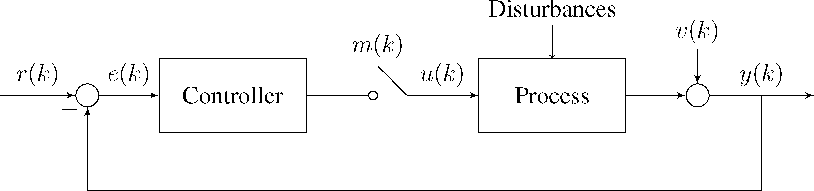
Consider the control loop in Figure 1, where at time k the operation mode m(k) ∈ {0, 1} denotes operation in either open-, or closed-loop denoted by the symbols 0 and 1 respectively. In manual mode, the input to the process u(k) is decided by the operator. In automatic mode, u(k) is given by the controller. The controller is driven by the control error e(k), formed from the setpoint r(k) subtracted by the measured process output y(k), which is corrupted by noise v(k). It is considered that the system can be described by an unknown model $ℳ$(θ), which is a function of the parameters θ.

A collection of data Z^N =[z(1)^T,⋯, z(N)^T]^T is available, where

$$z(k)=\left[m(k)r(k)u(k)y(k)\right].$$

(1)

The objective is to find time intervals Δ = [k_init, k_end] where the data in Z^N may be suitable to perform identification of the process parameters. Remark: if m(k) is not available, the mode is usually possible to infer from the behaviour of r(k) and u(k).

For its practical use, the following requirements are sought:

• Minimal knowledge about the plant is required. That is, none (or little) input is expected from the user.
• The resulting algorithm should process the data quickly. For example, a database containing data from a month of a large scale plant operation should not take longer than a few minutes to be processed.
• For each interval found, a numeric measure of its quality should be given. This can be used by the user in order to select which intervals to use for identification.

In order to achieve both Requirements 1 and 2, some simplifying assumptions are made:

Assumption 1.1 (SISO). Since the purpose is PID tuning it is assumed that only SISO control loops are to be estimated.

Assumption 1.2 (Linear models). It is assumed that the process can be well described by a linear model $ℳ$(θ).

Assumption 1.3 (Monotone step response). In process industry most uncontrolled processes are non-oscillatory, i.e., transfer functions with real valued poles are sufficient.

For a process in operation there are mainly two scenarios to hope for that may result in data informative enough for system identification (see [2]):

• The process is operating in manual mode and the input signal u(k) is varied enough to be exciting the process.
• The controller is in automatic and there are enough changes in the setpoint r(k) to make identification possible.

As a consequence, the method developed below is treating these two cases separately.

Notice that there are other scenarios that, at least in theory, would render a system in closed-loop identifiable. A longer discussion on this topic is given in next section.

2. Theoretical Guiding Principles and Preliminaries

To make this paper reasonably self-contained this section gives a brief review of the necessary system identification concepts needed to justify the design choices made. However, for a reader only interested in the final algorithm and its application this section may be omitted. The section is mainly based on [12–14].

Let each SISO loop correspond to a linear discrete-time system

$$\mathcal{S}:y(k)=G_0(q)u(k)+H_0(q)e(k).$$

(2)

where k is the sample index, q is the shift operator (qu(k) = u(k + T ) for the sampling interval T), e(k) is white noise with variance γ₀, y(k) is the output and u(k) is the input, which might be given in open-loop or by a stabilizing controller

$$u(k)=K(q)(r(k)-y(k))=S_0(q)K(q)r(k)-S_0(q)K(q)H_0(q)e(k),$$

(3)

where $S_0(q)\triangleq {(1+K(q)G_0(q))}^{-1}$ is the sensitivity function. The transfer functions G₀(q), H₀(q) and K(q) are rational and proper and H₀(q) is minimum phase and normalized such that H₀(∞) = 1. A parametric linear model structure $ℳ$(θ) is used to describe the system $\mathcal{S}$ as

$$ℳ\left(\mathrm{\theta }\right):y(k)=G(q,\mathrm{\theta })u(k)+H(q,\mathrm{\theta })e(k)$$

(4)

where θ ∈ ℝⁿ is the vector of unknown parameters. The true system S is said to belong to the model set $ℳ$≜{$ℳ$(θ)|θ ∈ D_θ} for some parameter set D_θ if there is θ′ ∈ D_θ such that $ℳ(\mathrm{\theta }\prime )=\mathcal{S}$. The equality here means that G₀(z) = G(z, θ′) and H₀(z) = H(z, θ′) for almost all z, i.e., the system and model are equivalent from an input-output relationship. The set defined by all θ′ such that $\mathcal{S}=ℳ(\mathrm{\theta }\prime )$ is denoted $D(\mathcal{S},ℳ)$ and contains a unique element θ₀, or “true pameters”, if the model structure is globally identifiable, the concept of identifiability will be reviewed in Section 2.2.

The optimal one-step ahead predictor for y(k) is given by

$$\widehat{y}(k|\mathrm{\theta })=H{\left(q,\mathrm{\theta }\right)}^{-1}G\left(q,\mathrm{\theta }\right)u(k)+\left(1-H{\left(q,\mathrm{\theta }\right)}^{-1}\right)y(k).$$

(5)

A sensible approach to find an estimate of the parameter, denoted $\widehat{\mathrm{\theta }}$, is to minimize the difference prediction errors, ε(k, θ) = y(k) − ŷ(k|θ) in some sense. As it will be reviewed in Section 2.3, if $\mathcal{S}\in ℳ$ and the data set is informative enough, prediction error methods will give consistent estimates of the parameter, i.e., $\widehat{\mathrm{\theta }}\in D(\mathcal{S},ℳ)$. Informative datasets are discussed in Section 2.2 and recursive prediction error methods are considered in Section 2.3.

One approach to find a model structure such that $\mathcal{S}\in ℳ$ is to derive the model from the laws of physics governing the processes and use the parameter vector θ to describe remaining unknown characteristics, e.g., the gain, poles or zeros. Since it would be impractical to consider knowledge of the dynamics for each loop in an entire process plant, we consider that no knowledge is available about the system (later on we will however assume the presence of integrators to be known). Instead, we seek for a flexible model structure that can describe a large set of system dynamics while allowing for an efficient identification procedure. Flexible and tractable black-box models are presented in Section 2.1.

The alternative models are called black-box since they are used to describe relations in the data and do not necessarily have parameters that relate to the original process. Flexible black-box models fit our purpose of finding data suitable for identification of process models. Notice that we are not aiming at directly finding a process model, with a clear physical interpretation or suitable for control purposes.

2.1. Black-Box Modeling with Laguerre Models

Because there is a one to one correspondence for the transfer functions in Equations (4) and (5) we focus the presentation for the predictor form and follow [13]. Assuming that H(q, θ) and G(q, θ) have the same unstable poles, it follows that the optimal predictor can be approximated as [15]

$$H{\left(z,\mathrm{\theta }\right)}^{-1}G\left(z,\mathrm{\theta }\right)\approx {\displaystyle \sum _{i=1}^n{b}_i{z}^{-1}\triangleq B_n(z)}$$

(6a)

$$H{\left(z,\mathrm{\theta }\right)}^{-1}-1\approx {\displaystyle \sum _{i=1}^n{a}_i{z}^{-i}\triangleq A_n(z)}.$$

(6b)

This approximation corresponds to an ARX model of order n and is exact as n → ∞. Therefore, high order ARX models can be used as flexible black-box models. An additional advantage is that the ARX model structure is linear in the parameters θ^T = [a₁,⋯, a_n, b₁,⋯b_n] and its identification in a prediction error sense is very tractable as will be discussed in Section 2.3.

There are a number of shortcomings with the parametrization in Equation (6) though. As noted by Wahlberg in [13], the rate of convergence for the approximation as n → ∞ is determined by the location of the poles of G(z, θ) which are not shared by H(z, θ) and the zeros of H(z, θ); the closer these are to the unit circle, the slower the approximation will converge. For sampled continuous-time systems, the continuous-time poles (and zeros) are mapped as e^pT and thus for a small sampling interval, T, the approximation will require large n. Similarly, for plants with an unknown delay d, it will require d/T additional coefficients for B_n(q).

An alternative parametrization that has a convergence rate of the approximation independent on T and which is more suitable for plants with a delay is possible with Laguerre polynomials as

$$H{\left(z,\mathrm{\theta }\right)}^{-1}G\left(z,\mathrm{\theta }\right)\approx {\displaystyle \sum _{i=1}^n{b}_i{L}_i(z,\mathrm{\alpha })\triangleq {\tilde{B}}_n(z,\mathrm{\alpha })}$$

(7a)

$$H{\left(z,\mathrm{\theta }\right)}^{-1}-1\approx {\displaystyle \sum _{i=1}^n{a}_i{L}_i(z,\mathrm{\alpha })\triangleq {\tilde{A}}_n(z,\mathrm{\alpha })}$$

(7b)

where L_i(q, α) is the ith Laguerre filter

$$L_i(q,\mathrm{\alpha })=\frac{\sqrt{\left(1-{\mathrm{\alpha }}^2\right)T}}{q-\mathrm{\alpha }}{\left(\frac{1-\mathrm{\alpha }q}{q-\mathrm{\alpha }}\right)}^{i-1}.$$

(8)

As for the ARX model, the approximation is exact when n → ∞. The distances of the Laguerre filter pole, 0 < α < 1, to the poles of the system determine the convergence rate for the approximation [13]. For fast convergence, α can be set as equal to the largest time constant in the system [16] but in case of scattered poles, the convergence may still be slow as discussed in [13]. Optimal choice of the Laguerre pole is discussed in [17].

The model structure in Equation (7) is a generalization of the model in Equation (6), which is retrieved for α = 0. In fact, introducing $\overline{\mathrm{\alpha }}=(1-\mathrm{\alpha })/T$ and δ = (q − 1)/T, Equation (8) can be rewritten as [13]

$$\frac{{\mathrm{\delta }}^{i-1}}{{\left(1+\mathrm{\delta }/\overline{\mathrm{\alpha }}\right)}^n},$$

(9)

so the Laguerre model reduces to an ARX model with a prefilter $1/{(1+\mathrm{\delta }/\overline{\mathrm{\alpha }})}^n$ in the δ domain.

The Laguerre filter of order i consists of one low-pass filter cascaded with (i − 1) first-order all pass filters, which acts effectively as a delay approximation of order (i − 1). The substitution of the delay operator in an ARX model with a Laguerre filter has important characteristics to allow for an accurate description and of low order [13]. The maximum delay $\overline{d}$ a Laguerre model can explain can be found by comparing a Padé approximation of a delay with the all pass part of the Laguerre filters [18,19] and is given by

$$\overline{d}=-2(n-1)T/\log \mathrm{\alpha }.$$

(10)

If the real pole α and order n are selected properly, Laguerre models can efficiently approximate a large class of linear systems [2]. In general, the performance of the identification is relatively insensitive to the choice of α [10,20]. Estimation of α from data is presented in, for example, [21], but this has not been found necessary in this paper.

Because a Laguerre model has a finite gain at low frequencies, it is not a good approximation for plants with an integrator. This is in fact an important limitation of Laguerre models since many processes in process industry (most notably level control) have an integrating behavior. To overcome this we will treat integrating loops separately as described later in Section 3.

Another limitation is that the poles for the Laguerre filter are real and for resonant processes the approximation may take long to convergence. An alternative is to consider the use of complex poles in the expansion with, e.g., Kautz polynominals. See [22] for details.

2.2. Identifiability, Informative Data Sets and Persistence of Excitation

After selection of an adequate model structure, one might ask whether it is possible to unequivocally identify its parameters from the data using a prediction error method. Whether this is possible will depend on properties of both the model structure and of the data set used. Recalling there is a one to one relation between the optimal predictor in Equation (5) and the model in Equation (4), we study this question based on the predictor form. Following [12,23] we introduce the shorthand notation,

$$\widehat{y}(k|\mathrm{\theta })=\underset{\triangleq W(q,\mathrm{\theta })}{\underbrace{\left[H{\left(q,\mathrm{\theta }\right)}^{-1}G\left(q,\mathrm{\theta }\right)\left(1-H{\left(q,\mathrm{\theta }\right)}^{-1}\right)\right]}}\underset{\triangleq z(k)}{\underbrace{\left[\begin{array}{c}u(k)\\ y(k)\end{array}\right]}}=W(q,\mathrm{\theta })z(k).$$

(11)

First, it will not be possible to distinguish two different parameters, θ ≠ θ′, if the related linear filters are the same i.e., W (z, θ) = W (z, θ′). Identifiability of a model structure at θ′ ∈ D_θ is thus defined as whether

$$W(z,\mathrm{\theta })=W(z,\mathrm{\theta }\prime ),\forall z\Rightarrow \mathrm{\theta }={\mathrm{\theta }}^{\prime }$$

(12)

in a region (locally identifiable) or for any θ (globally identifiable). Notice that if $\mathcal{S}\in ℳ$ and the model is globally identifiable $D(\mathcal{S},ℳ)={\mathrm{\theta }}_0$. Furthermore, the ARX model structure is strictly globally identifiable, i.e., it is globally identifiable at any θ′ ∈ D_θ.

Even if the model is globally identifiable, the parameters may not be retrievable depending on the data z(k), take for instance z(k) = 0. This leads to a definition of informative datasets, which allows for a distinction of different parameters in the model set. For what follows, we say that a signal ϕ(k) is quasi-stationary if it satisfies

$$\begin{array}{ccc}E\mathrm{\varphi }(k)=m_{\mathrm{\varphi }}(k),& |m_{\mathrm{\varphi }}(k)|\le C,& \forall k\end{array}$$

(13a)

$$\begin{array}{cc}E\mathrm{\varphi }(k)\mathrm{\varphi }(r)=R_{\mathrm{\varphi }}(k,r),& |R_{\mathrm{\varphi }}(k,r)|\le C\end{array}$$

(13b)

$$\begin{array}{cc}\overline{E}{R}_{\mathrm{\varphi }}(k,k-\mathrm{\tau })=R_{\mathrm{\varphi }}(\mathrm{\tau }),& \forall \mathrm{\tau },\end{array}$$

(13c)

where

$$\overline{E}f(k)\triangleq \underset{N\to \infty }{\lim }\frac{1}{N}{\displaystyle \sum _{k=1}^{N}Ef(k).}$$

(14)

The expectation in Equation (13) applies only for stochastic parts. For deterministic signals the expectation is dropped and the definition means that ϕ(k) is a well-defined, bounded, sequence.

A quasi-stationary data-sequence ${\{z(k)\}}_1^N$ is informative enough with respect to a model set $ℳ$ if it allows for the distinction between any two models W(z, θ₁), W(z, θ₂) in the set, i.e.,

$$\overline{E}{\left[(W(z,{\mathrm{\theta }}_1)-W(z,{\mathrm{\theta }}_2))z(k)\right]}^2=0\Rightarrow W(e^{\mathrm{\iota }\mathrm{\omega }},{\mathrm{\theta }}_1)\equiv W(e^{\mathrm{\iota }\mathrm{\omega }},{\mathrm{\theta }}_2)$$

(15)

for almost all ω. Notice that this definition depends only on the model set and not on the true system. To illustrate the consequence of this definition to signals, we define

Definition 1 (Persistent excitation). A quasi-stationary regressor ϕ(k) is persistently exciting (PE) if Ē[ϕ(k)ϕ(k)^T]>0.

Definition 2 (Richness of a signal). A scalar quasi-stationary signal u(k) is sufficiently rich of order n (SRn) if ϕ(k)^T = [u(k − 1),⋯, u(k − n)] is PE.

As discussed, informativeness of a data set depends on the model structure used. We review the conditions on the data for open and closed loop for ARX models, analogous results are possible for the ARX-Laguerre model using the δ representation given in Equation (9) with a prefilter. Let the ARX model in Equation (6) have polynomials $A_{n_a}(q)$ and $B_{n_b}(q)$, then the following results apply [23].

Theorem 1 (ARX, open loop). Let the system be operating in open-loop, the data set is informative if and only if u(k) is SRn_b.

Therefore, for the open loop case, the input signal must be rich enough. The closed loop case was studied already by Söderström, Gustavsson and Ljung [24]. It turns out that the system may be identifiable even if the setpoint is zero, provided the controller is complex enough. A number of such scenarios are discussed in [12]; nonlinear control, switching linear controllers or fixed linear controller with high enough order. The case of fixed linear controllers is further studied in [14]. Distinguish between two cases, either r(k) ≡ 0, i.e., the system is driven solely by the noise, or r(k) is changing. We denote the first situation as a controller operation for disturbance rejection and the second as a servo operation. Let the feedback stabilizing controller given in Equation (3) be given in a coprime factorization $K(z)=\frac{X(z^{-}{}^1)}{Y(z^{-1})}$ where the polynomials are $X(z^{-1})=x_0+x_1{z}^{-1}+\cdots +x_{n_x}{z}^{-n_x}$ and $Y(z^{-1})=1+y_1{z}^{-1}+\cdots +y_{n_x}{z}^{-n_y}$. Then the following resuls apply [14]:

Theorem 2 (ARX, servo). Let max(n_x − n_a, n_y − n_b) < 0, the data are informative for almost all SRn_r r(k), if and only if n_r ≥ min(n_a − n_x, n_b − n_y).

Theorem 3 (ARX, disturbance rejection). Let r(k) ≡ 0, then the data are informative if and only if max(n_x − n_a, n_y − n_b) ≥ 0.

In [25], more general results are given for general linear plants with a delay and considers possible pole-zero cancellations. These theorems above give a minimal set of conditions on the inputs to allow for a distinction of the parameters from the data. The result in Theorem 3 indicates that it is possible to find the parameters based on the excitation from the noise if the controller has high enough order compared to the model. For a model structure of high order, and controlled by PID controllers, it is clear that this condition will hardly hold. In this case, the information contained in the reference must complement the simplicity of the controller as given by Theorem 2.

The following are more general results which apply to general linear models. Defining the spectrum of a signal ϕ(k) as

$${\mathrm{\Phi }}_{\mathrm{\varphi }}(\mathrm{\omega })\triangleq {\displaystyle \sum _{\mathrm{\tau }=-\infty }^{\infty }{R}_{\mathrm{\varphi }}(\mathrm{\tau })e^{-\mathrm{\iota }\mathrm{\tau }\mathrm{\omega }}},$$

(16)

a signal is said persistently exciting if its spectrum Φ_ϕ(ω) > 0 for almost all ω. The next results follow for any linear plant [12],

Theorem 4 (Open loop). A persistently exciting input u(k) is informative enough for open loop experiments.

Theorem 5 (Closed loop). A persistently exciting reference r(k) is informative enough for closed loop experiments.

So, in general terms, for open-loop (closed-loop) there should be enough changes in the input (reference) to allow for an identification of any linear plant.

2.3. (Recursive) Prediction Error Methods

An important feature of the general predictors given by the approximations in Equations (6) or (7) is that they can be written as linear regressions,

$$\widehat{y}(k|\mathrm{\theta })={\mathrm{\phi }}^T(k)\mathrm{\theta },$$

(17)

where φ^T (k) is function of past inputs u(k − 1),…, u(1) and outputs y(k − 1),…, y(1). In a linear regression, the parameters θ ∈ ℝⁿ appear as a linear function with the regressors, which allow for a simple identification procedure. A common choice of identification approach is the prediction error method, where the prediction error ε(k, θ) = y(k) − ŷ(k|θ) = y(k) − φ(k)^T θ is minimized according to some criterion. To reduce the storage requirements of the resulting algorithm and to allow for adaptive solutions, recursive methods are preferred, which can be updated in a data stream. Many recursive prediction error methods are possible, see, e.g., [12]. For the presentation here, we consider an exponentially weighted quadratic prediction error criterion, where the estimate is given as

$${\widehat{\mathrm{\theta }}}_k=\arg \underset{\mathrm{\theta }\in D_{\mathrm{\theta }}}{\min }{V}_k(\mathrm{\theta })=\arg \underset{\mathrm{\theta }\in D_{\mathrm{\theta }}}{\min }{\displaystyle \sum _{i=1}^k{\mathrm{\lambda }}^{k-1}{\mathrm{\epsilon }}^2(k,\mathrm{\theta }),}$$

(18)

with 0 < λ < 1. Direct minimization gives the solution for this problem in closed form, which can be written recursively as [12],

$${\widehat{\mathrm{\theta }}}_k={\widehat{\mathrm{\theta }}}_{k-1}+\overline{R}{\left(k\right)}^{-1}\mathrm{\phi }(k)\mathrm{\epsilon }(k,{\widehat{\mathrm{\theta }}}_{k-1})$$

(19a)

$$\overline{R}\left(k\right)=\mathrm{\lambda }\overline{R}(k-1)+\mathrm{\phi }(k)\mathrm{\phi }{\left(k\right)}^T$$

(19b)

$$V_k({\widehat{\mathrm{\theta }}}_k)=\mathrm{\lambda }{V}_{k-1}({\widehat{\mathrm{\theta }}}_{k-1})+\mathrm{\epsilon }(k,{\widehat{\mathrm{\theta }}}_{k-1})\mathrm{\epsilon }(k,{\widehat{\mathrm{\theta }}}_k).$$

(19c)

This algorithm is known as the Recursive Least Squares (RLS). The feasibility of Equation (19a) depends on whether the information matrix$\overline{R}(k)$ is invertible, i.e., the matrix must be full-rank.

2.3.1. Frequency Description of Prediction Error

Some important properties of prediction error methods can be highlighted with a description in the frequency domain. To illustrate this, we replace the exponential weighting function λ^k−i in Equation (18) by the constant weight $\frac{1}{2N}$, where N is the number of data samples, and let N → ∞. The limiting cost is denoted $\overline{V}(\mathrm{\theta })$ and it follows from the definition of the Fourier transform and Equation (16) that

$$\overline{V}(\mathrm{\theta })\triangleq \underset{N\to \infty }{\lim }\frac{1}{2N}{\displaystyle \sum _{k=1}^N{\mathrm{\epsilon }}^2(k,\mathrm{\theta })=\overline{E}\frac{1}{2}{\mathrm{\epsilon }}^2}(k,\mathrm{\theta })=\frac{1}{4\mathrm{\pi }}{\displaystyle {\int }_{-\mathrm{\pi }}^{\mathrm{\pi }}{\mathrm{\Phi }}_{\mathrm{\epsilon }}(\mathrm{\omega },\mathrm{\theta })d\mathrm{\omega }.}$$

(20)

Using the shorthand notation G₀, H₀ to describe the system’s transfer functions in Equation (2) and G_θ, H_θ to describe the transfer functions of the model in Equation (4), it follows, see [12], that the residuals’ spectrum can be written as

$${\mathrm{\Phi }}_{\mathrm{\epsilon }}(\mathrm{\omega },\mathrm{\theta })=\frac{{|G_0+B_{\mathrm{\theta }}-G_{\mathrm{\theta }}|}^2}{{|H_{\mathrm{\theta }}|}^2}{\mathrm{\Phi }}_u+\frac{{|H_0-H_{\mathrm{\theta }}|}^2}{{|H_{\mathrm{\theta }}|}^2}\left({\mathrm{\gamma }}_0\frac{{|{\mathrm{\Phi }}_{ue}|}^2}{{\mathrm{\Phi }}_u}\right)+{\mathrm{\gamma }}_0,$$

(21a)

$$B_{\mathrm{\theta }}=(H_0-H_{\mathrm{\theta }})\frac{{\mathrm{\Phi }}_{ue}}{{\mathrm{\Phi }}_u},$$

(21b)

where the inputs were dropped for compactness and Φ_ue denotes the cross-spectrum of u and e, defined in an analogy to Equation (13). The expression allows us to study the effects of the model chosen and excitation to the cost function and thus to the estimated parameters. Notice for instance that if $\mathcal{S}\in ℳ$, θ′ minimizes the criterion. Furthermore, G_θ will be pushed towards (G₀ + B_θ), and for that reason B_θ will introduce a bias to the estimate of G₀.

For open-loop experiments, the input u is uncorrelated with the noise e so Φ_ue ≡ 0 and so the bias term B_θ ≡ 0. The input spectra ϕ_u will thus control the frequencies where ${|G_{\widehat{\mathrm{\theta }}}-G_0|}^2$ is minimized. For instance, some times the noise model is unimportant and thus fixed to a constant, i.e., H(q, θ) = H_*(q), this was used in our previous paper [9]. In this case we have

$$\arg \underset{\mathrm{\theta }}{\min }\overline{V}(\mathrm{\theta })=\arg \underset{\mathrm{\theta }}{\min }{\displaystyle {\int }_{-\mathrm{\pi }}^{\mathrm{\pi }}{|G_0-G_{\mathrm{\theta }}|}^2\frac{{\mathrm{\Phi }}_u}{{|H_{*}|}^2}d\mathrm{\omega },}$$

(22)

and the minimizing argument is such that the distance |G_θ−G₀|² is decreased according to the frequency weight given by the ratio of the input spectrum Φ_u and the noise model chosen |H_*|². Furthermore, the relevance of a persistently exciting input becomes clear in the expression.

For the closed-loop case, u will be correlated to e leading to non-zero Φ_ue and thus the bias term B_θ should be addressed by adjusting the noise model H_θ to H₀. Splitting the input spectrum into the parts originating from the reference r and noise e as ${\mathrm{\Phi }}_u(\mathrm{\omega })={\mathrm{\Phi }}_u^r(\mathrm{\omega })+{\mathrm{\Phi }}_u^e(\mathrm{\omega })$, if the input can be written as u(k) = K₁(q)r(k) + K₂(q)e(k), then ${|{\mathrm{\Phi }}_{ue}\left(\mathrm{\omega }\right)|}^2={\mathrm{\gamma }}_0{\mathrm{\Phi }}_u^e(\mathrm{\omega })$ and

$$\arg \underset{\mathrm{\theta }}{\min }\overline{V}(\mathrm{\theta })=\arg \underset{\mathrm{\theta }}{\min }{\displaystyle {\int }_{-\mathrm{\pi }}^{\mathrm{\pi }}\frac{{|G_0+B_{\mathrm{\theta }}-G_{\mathrm{\theta }}|}^2}{{|H_{\mathrm{\theta }}|}^2}{\mathrm{\Phi }}_u+{\mathrm{\gamma }}_0\frac{{|H_0-H_{\mathrm{\theta }}|}^2}{{|H_{\mathrm{\theta }}|}^2}\frac{{\mathrm{\Phi }}_u^r}{{\mathrm{\Phi }}_u}d\mathrm{\omega },}$$

(23a)

and the bias contribution follows as

$${|B_{\mathrm{\theta }}|}^2={|H_0-H_{\mathrm{\theta }}|}^2\frac{{\mathrm{\gamma }}_0}{{\mathrm{\Phi }}_u}\frac{{\mathrm{\Phi }}_u^e}{{\mathrm{\Phi }}_u}.$$

(23b)

The equation shows that fixing the noise model for a system operating in closed loop will lead to a biased estimate of G₀. Furthermore, for a controller in disturbance rejection mode, with ${\mathrm{\Phi }}_u^r\equiv 0$, the bias can only be controlled by the ratio of the noise energy and the contribution of the noise to the input energy due to feedback, i.e., ${\mathrm{\gamma }}_0/{\mathrm{\varphi }}_u^e$. So to reduce the bias, the influence of the noise to the input should increase, which contradicts many control objectives. Reducing the bias for a system operating in disturbance rejection mode is therefore difficult. In servo mode, the reference r can reduce |H₀ − H_θ|² through the ratio ${\mathrm{\Phi }}_u^r/{\mathrm{\Phi }}_u$, thus reducing the bias term.

2.3.2. Asymptotic Properties of the RLS

Assume that the system in Equation (2) is in the model set, i.e., $\mathcal{S}\in ℳ$, and that the data are informative enough then as λ → 1 and k → ∞,

$$\sqrt{1-\mathrm{\lambda }}({\widehat{\mathrm{\theta }}}_k-{\mathrm{\theta }}_0)\in As\mathrm{N}(0,P_{\mathrm{\theta }}),P_{\mathrm{\theta }}\triangleq \frac{1}{2}{\mathrm{\gamma }}_0{\overline{R}}^{-1},\overline{R}\triangleq \overline{E}\left[\mathrm{\phi }(k)\mathrm{\phi }{(k)}^T\right]$$

(24)

so the asymptotic estimate is consistent and is distributed according to a Gaussian distribution. The covariance matrix is given by

$${\sum }_{\mathrm{\theta }}\triangleq E\left[({\widehat{\mathrm{\theta }}}_k-{\mathrm{\theta }}_0){({\widehat{\mathrm{\theta }}}_k-{\mathrm{\theta }}_0)}^T\right]~\frac{(1-\mathrm{\lambda })}{2}{\mathrm{\gamma }}_0{\overline{R}}^{-1},$$

(25)

which is controlled by $\overline{R}$. In order to make the covariance small, $\overline{R}$ should be made large in some sense. This idea is explored, for instance, in experiment design (choosing u) for system identification. The asymptotic result in Equation (24) will provide useful guidance when defining our algorithm in the next section.

For finite sample, we can replace $\overline{R}$ and γ₀ with their sample estimates, given by

$${\widehat{\mathrm{\gamma }}}_k=(1-\mathrm{\lambda })V_k({\widehat{\mathrm{\theta }}}_k),{\widehat{\overline{R}}}_k=(1-\mathrm{\lambda })\overline{R}(k),$$

(26a)

and so the sample covariance matrix is given by

$${\widehat{\mathrm{\Sigma }}}_k=\frac{(1-\mathrm{\lambda })}{2}{\widehat{\mathrm{\gamma }}}_k{\overline{R}}_k^{-1}=\frac{(1-\mathrm{\lambda })}{2}{V}_k({\widehat{\mathrm{\theta }}}_k)\overline{R}{(k)}^{-1}.$$

(26b)

3. User Choices, Data Features

Based on the theoretical guiding principles outlined, we describe and motivate the choices leading to the proposed algorithm. The main ingredients are the choice of a flexible black-box model structure, followed by the definition of data features and test to indicate and quantify the quality of the data to retrieve a linear model. Through the section, choices are made taking into consideration reduced complexity, implementation aspects and tuning.

The algorithm is outlined in Section 4 and for a recursive implementation, based on a data stream. Two basic pre-processing steps are required. First, the signals are considered to be normalized (scaled) between 0 and 1. This is important to simplify the tuning and because some of the features are sensitive to scaling. An adequate scaling is possible if the range for the variables is available, which is normally the case in the process industry. Furthermore, we remove the first sample, of the data stream, from r(k), u(k) and y(k) since we are working with linear models. To avoid confusion, the transformed variables are denoted with a ·′ symbol whenever important. Four tests of increasing complexity are used which are checked in cascade and notation which is relevant to the implementation will be introduced through the section.

3.1. Choice of Model Structure

While by Assumption 1.2 it is considered that the loops in the plant can be described by a linear model as given in Equation (2), it would be too restricting to consider available knowledge of a model structure $ℳ$(θ) for each SISO loop in an entire plant. Since our objective with the algorithm is not to find a process model but rather to find segments of data from where a process model can be retrieved, it is natural to avoid including knowledge of the models for each loop and to instead use flexible black-box models when searching for data. From the discussion presented in Section 2.1, flexible and tractable (i.e., allowing for a representation as a linear regression given by Equation (17)) linear models can be achieved with high-order ARX as in Equation (6) and high order ARX-Laguerre models as in Equation (7).

As discussed, the Laguerre representation presents important advantages, it will often require lower order models for the same quality of the approximation and it is more suitable for processes with a delay since the delay operator is replaced by the Laguerre filters, acting as a delay approximation. The later feature is critical in the process industry as many loops contain nonzero delays. A Laguerre expansion is thus used to model the input relation, i.e.,

$$H{\left(z,\mathrm{\theta }\right)}^{-1}G\left(z,\mathrm{\theta }\right)\approx {\displaystyle \sum _{i=1}^{n_b}{b}_i{L}_i(z,\mathrm{\alpha }).}$$

(27a)

For the noise model, we do not expect any delays. Since the use of a Laguerre model requires the additional computational complexity for the filtering operations, we choose a noise model based on the expansion on lags as in Equation (6), i.e.,

$$H{\left(z,\mathrm{\theta }\right)}^{-1}-1\approx {\displaystyle \sum _{i=1}^{n_a}{a}_i{z}^{-i}.}$$

(27b)

The predictor can be written as a linear regression given by Equation (17) with

$$\mathrm{\phi }{\left(k\right)}^T=\left[{\tilde{u}}_1(k)\cdots {\tilde{u}}_{n_b}(k)y(k-1)\cdots y(k-n_a)\right]$$

(28a)

$${\mathrm{\theta }}^T=\left[b_1\cdots b_{n_b}{a}_1\cdots a_{n_a}\right]=\left[{\left({\mathrm{\theta }}^b\right)}^T{\left({\mathrm{\theta }}^a\right)}^T\right],$$

(28b)

where û_i(k) ≜ L_i(q, α)u(k). The resulting model presents the key characteristics

• for an adequate choice of model orders n_b, n_a, it is a flexible representation of any linear system,
• for an adequate choice of α lower orders n_b are possible compared to high-order ARX because of the use the Laguerre polynomials to describe the input relations,
• it can be written as a linear regression which allows for an efficient identification, using, e.g., the RLS algorithm.

These features are instrumental for the method proposed in this paper.

3.1.1. Tuning

The use of the Laguerre representation requires the choice of the model order n, and the Laguerre filter pole, α. As discussed in Section 2.1, α will control the convergence rate of the approximation and for a fast convergence one can set equal to the largest time constant present. Once α is chosen, the maximum delay $\overline{d}$ the Laguerre filters can approximate is given by Equation (10). With knowledge of the maximum delay possible in the plant or an upper bound for it, the model order n_b can be chosen as

$$n_b\ge \lceil \frac{-\overline{d}\log \mathrm{\alpha }}{2}+1\rceil ,$$

(29)

where ⌈·⌉ denotes the ceiling operation.

3.1.2. Plants with an Integrator

To overcome the limitation of a Laguerre model having a finite gain at zero frequency, it is assumed known if an integrator is present in each loop. The input is then integrated as

$$\overline{u}(k)=\frac{u^{\prime }(k)}{(1-q^{-1})},$$

(30)

and ū(k), y′(k) are used in the identification instead. As found in [10], since the main dynamics for integrating plants relates to the integrators themselves, the pole of the Laguerre filters α for integrating plants can be made considerably smaller (faster) than for non-integrating plants. The Laguerre pole for integrating plants is denoted here as α_I. The same model order n for non-integrating plants can be used or a specific choice n_I can be made for integrating plants, e.g., using Equation (29) with α_I.

3.2. Choice of Operational Modes to Consider

Based on the discussion on informative datasets in Section 2.2, there are three main modes of operation of a plant, open-loop and closed-loop in servo or disturbance rejection operation. For operation in disturbance rejection mode, with r(k) ≡ 0, even if the condition on controller order in Theorem 3 is fullfilled, it only guarantees that the information matrix is full rank while its numerical conditioning might be poor. The identification in disturbance rejection mode is in general challenging as discussed in Section 2.3.1. To further illustrate this, consider the frequency representation of Equation (23), where the bias term is controlled by ${\mathrm{\gamma }}_0/{\mathrm{\Phi }}_u^e$ when r(k) ≡ 0, i.e., ${\mathrm{\Phi }}_u^r\equiv 0$. For a closed-loop system given by Equation (3), ${\mathrm{\Phi }}_u^r={|S_0|}^2{|K|}^2{|G_0|}^2{\mathrm{\gamma }}_0$ and thus the bias can be reduced by increasing the sensitivity function gain. This directly contradicts with the control objective of disturbance rejection, where the sensitivity function should be made small. This is also the practical experience by the authors that, even if first-order models are identified, closed loop identification with a constant setpoint very rarely leads to useful models. See [8,26] for simulation examples where the disturbance rejection case is considered for process identification.

As already presented in the Problem Formulation this has influenced us to only look for intervals where the input r (or u for the open-loop case) is in fact moving. We consider theoretically based tests in Sections 3.4 and 3.5. Before proceeding though, we develop two heuristic tests that will help to reduce the overall evaluation time for the algorithm.

3.3. Simple Heuristic Tests

Process plants often operate in steady-state. Except for the disturbance rejection operation, which is not considered further, there must be some change in the inputs u or r in open- or closed-loop respectively if any process model is to be retrieved. After a change in the input, it is also expected that the output will be varying after some time, only if these two events are observed can one expect to be able to retrieve a process model from the input-output data. Checking for changes in the input and for the variability of the output are computationally cheap and can thus be useful to reduce the amount of computations required to scan large datasets. We discuss two approaches of how this can be achieved.

3.3.1. Input Step Change Test

The operation of process plants with the changes of setpoints and eventual open-loop operation is often done through step changes. This is in fact the case for the evaluation example presented in Section 5. For ease of notation, we define

$$\mathrm{\zeta }(k)\triangleq \neg m(k)u^{\prime }(k)+m(k)r^{\prime }(k)$$

(31)

so that ζ(k)=u′(k) in case of an open-loop operation and ζ(k)=r′(k) in case of closed-loop operation. A step change of size η₁ can be detected with a threshold check

$$|\mathrm{\zeta }(k)|>{\mathrm{\eta }}_1,$$

(32)

for a change larger than η₁. The threshold η₁ should be chosen very small as this test is only used to avoid scanning for steady-state data.

3.3.2. Variability of y Test

Once a change in the input has been detected, one can check for reasonably sized variations of y before applying more computationally demanding tests. To reduce memory requirements and to allow for adaptability, the variance of y can be computed recursively with an exponential moving average. Denoting µ_y(k) as an estimate for the mean and γ_y(k) as an estimate for the variance, a recursive estimate can be found by [27]

$${\mathrm{\mu }}_y(k)={\mathrm{\lambda }}_{\mathrm{\mu }}{y}^{\prime }(k)+(1-{\mathrm{\lambda }}_{\mathrm{\mu }}){\mathrm{\mu }}_y(k-1)$$

(33a)

$${\mathrm{\gamma }}_y(k)=\frac{2-{\mathrm{\lambda }}_{\mathrm{\mu }}}{2}\left({\mathrm{\lambda }}_y{\left(y^{\prime }(k)-{\mathrm{\mu }}_y(k)\right)}^2+(1-{\mathrm{\lambda }}_{\mathrm{\lambda }}){\mathrm{\gamma }}_y(k-1)\right)$$

(33b)

which is tested with a threshold check

$${\mathrm{\gamma }}_y(k)>{\mathrm{\eta }}_2$$

(33c)

where 0 < λ_µ, λ_γ < 1 are the forgetting factors, controlling the effective size of the averaging window for the estimation of the mean and variance of y respectively. Since y′ is normalized between 0 and 1, the threshold η₂ can be chosen relative to its range, e.g., η₂ = 0.01² means a standard deviation of 1% relative to the output range.

3.4. Finding Excitation in the Data

More theoretically based criteria are possible based on the conditions for informative datasets of Theorems 1 and 2. Checking whether the inputs are sufficiently rich is however impractical since the definition of persistent excitation is based on an ensemble of potential observations, with the Ē operator given in Equation (14). Furthermore, many signals used in practice, during the operation of the plant, are of low SRn. As an example, consider a unit step (Heaviside step) change u(k) = H(k), with H(k) = {1 if k ≥ 0, 0 otherwise}, let ϕ(k) = [H(k − 1),…, H(k − n)] as in Definition 2 and note that the rank of

$$\overline{E}[\mathrm{\varphi }(k)\mathrm{\varphi }{\left(k\right)}^T]=\underset{N\to \infty }{\lim }\frac{1}{N}\left[\begin{array}{cccc}N& N-1& \cdots & N-n\\ N-1& N-2& \dots & N-n\\ ⋮& \ddots & \cdots & ⋮\\ N-n& N-n& \cdots & N-n\end{array}\right]=\left[\begin{array}{cc}1& 0\\ 0& 0\end{array}\right]$$

(34)

is 1 for any n and a step is thus SR1. This is true even though the matrix is full rank for finite N and it would be possible to compute an estimate. Instead of attempting to check for persistence of excitation, we check whether it is possible to compute an estimate of the parameters.

Considering an estimate based on the recursive least squares in Equation (19), note that the paremeter estimate in Equation (19a) corresponds to solving the linear system

$$\overline{R}(k)\mathrm{\Delta }\mathrm{\theta }=\mathrm{\phi }(k)\mathrm{\epsilon }(k,{\widehat{\mathrm{\theta }}}_{k-1})$$

(35)

and updating the estimate as ${\widehat{\mathrm{\theta }}}_k=\mathrm{\Delta }\mathrm{\theta }+{\widehat{\mathrm{\theta }}}_{k-1}$. A necessary condition for the solution is that the information matrix $\overline{R}(k)$ is full-rank. A rank test, however, gives little information about the numerical condition of $\overline{R}(k)$. If $\overline{R}(k)$ is ill-conditioned small perturbations to the right-hand side of Equation (35) (or to $\overline{R}(k)$) can lead to large errors to the estimate. A more suitable test is to check for its condition number which is described next.

Numerical Conditioning of $\overline{R}(k)$ Test

Numerical conditioning of a linear system of equation Ax = b can be assessed as follows. Introduce a perturbed linear system A(x + Δx) = (b + Δb), then it follows that (see e.g., [28]),

$$\frac{{\Vert \mathrm{\Delta }x\Vert }_p}{{\Vert x\Vert }_p}\le {\kappa }_p(A)\frac{{\Vert \mathrm{\Delta }b\Vert }_p}{{\Vert b\Vert }_p},{\kappa }_p(A)\triangleq {\Vert A\Vert }_p{\Vert A^{-1}\Vert }_p,$$

where κ_p(A) ≥ 1 is the condition number of matrix A. Small values of

$${\kappa }_p(k)\triangleq {\kappa }_p(\overline{R}(k))$$

(36)

are thus desirable in order to improve the reliability of the solution to numerical errors. Any p-norm can be used, the commonly chosen 2-norm gives,

$${\kappa }_2(A)=\frac{{\mathrm{\sigma }}_{\max }(A)}{{\mathrm{\sigma }}_{\min }(A)},$$

(37)

with σ_max(A) and σ_min(A) denoting the largest respectively smallest singular values of A.

Because σ_min can be close to zero, κ(k) can vary between [1, ∞) and it might be difficult to set a threshold for it. An alternative is to monitor its inverse, also known as the reciprocal condition number as it will have values in [0, 1]. Notice that when using the reciprocal condition number, high values relate to good conditioning. The reciprocal condition number is tested with a threshold

$${\kappa }_2^{-1}(k)>{\mathrm{\eta }}_3.$$

(38)

The condition number has been suggested as measure of data excitation already in [9] and is commonly used to monitor the reliability of the solution of a linear system, see e.g., [18]. In [8], the authors note that the condition number for step changes will often be large, which can be seen from the finite sample matrix in Equation (34). They suggest a choice of threshold in the order of 10⁴, i.e., 10⁻⁴ when using its reciprocal. We note that increasing the model orders may increase the number of small eigenvalues in $\overline{R}(k)$ due to over-fitting and thus η₃ may be chosen proportional to the number of estimated parameters.

3.5. Granger Causality Test

Notice, however, that the condition number is scaling independent. Hence even if the the condition number is low it says nothing about the magnitude of the excitation compared to the noise. Therefore, it is necessary to also check there there is in fact a noticeable correlation between input and output. A more conclusive test would be to verify whether there is a causal relation between the input u and the output y. If there is a casual relation between the variables, it is reasonable that y(t) can be predicted better making use of past input-output data, ${\{u(k),y(k)\}}_1^{t-1}$ than it would be predicted by using only ${\{y(k)\}}_1^{t-1}$. This relates to the concept of Granger causality, see [29] for example.

For the black-box model used here given in regressor form by Equation (28), if u(k) Granger-causes y(k), it must be that some of the parameters relating to the input-output relation is non-zero, i.e., ${\widehat{\mathrm{\theta }}}_b\ne 0$. We can thus define a null hypothesis $\mathscr{H}$₀ : θ_b = 0 which should be rejected in case there is a Granger-causal relation present. A statistical test for this hypothesis is readily available from the asymptotic results for the estimate $\widehat{\mathrm{\theta }}$ given by Equation (24) since under the null hypothesis $\mathscr{H}$₀,

$${\left({\widehat{\mathrm{\theta }}}_k^b\right)}^T{\left({\sum }_{\mathrm{\theta }}^b\right)}^{-1}{\widehat{\mathrm{\theta }}}_k^b\in As{\mathrm{\chi }}_{n_b},$$

(39)

where (Σ^b)⁻¹ is the inverse of the sub matrix of Σ_θ associated to θ_b only and χ_d is the chi square distribution with d degrees of freedom. The statistics can be computed based on the finite sample estimates in Equation (26), giving

$$s(k)\triangleq {\left({\widehat{\mathrm{\theta }}}_k^b\right)}^T{\left({\widehat{\mathrm{\Sigma }}}_k^b\right)}^{-1}{\widehat{\mathrm{\theta }}}_k^b$$

(40)

The null hypothesis is rejected if

$$s(k)>{\mathrm{\eta }}_4,{\mathrm{\eta }}_4\triangleq \arg \underset{\mathrm{\eta }}{\inf }\left\{\mathrm{\eta }\in ℝ:{\displaystyle {\int }_{-\infty }^{\mathrm{\eta }}{\mathrm{\chi }}_{n_b}(x)dx>p}\right\}$$

(41)

where the threshold η₄ is taken as the p quantile of ${\mathrm{\chi }}_{n_b}$. This condition must be satisfied in our algorithm to assign a data interval as useful.

The statistic s(k) can also be seen as a measure of data quality since the larger it is, the more evidence there is in the data of a causal relation between u and y. This quantity can therefore be used to rank the quality of the various intervals that are found, larger meaning better.

As discussed in Section 3.4 however, the standard implementation of the RLS filter given in Equation (19) requires inversion of $\overline{R}(k)$ which may lead to numerical problems. The problem of ill conditioning can be reduced with an alternative implementation choice based on the QR factorization, which gives better numerical conditioning of the solution. This is described next.

Choice of Implementation of RLS Based on the QR Factorization

For k data points, the recursive least squares with a forgetting factor λ can be written as

$${\widehat{\mathrm{\theta }}}_k=\arg \underset{\mathrm{\theta }}{\min }{V}_k(\mathrm{\theta })=\arg \underset{\mathrm{\theta }}{\min }{\Vert \mathrm{\Lambda }{\left(k\right)}^{1/2}(Y(k)-\mathrm{\varphi }(k)\mathrm{\theta })\Vert }_2^2$$

(42)

where Λ(k) is a diagonal matrix with [Λ(k)]_ii = λ^k−i and

$$Y{\left(k\right)}^T=\left[y(1)\cdots y(k)\right],\mathrm{\varphi }{\left(k\right)}^T=\left[\mathrm{\phi }(1)\cdots \mathrm{\phi }(k)\right].$$

(43)

Because the norm in the minimization is not affected by an orthonormal transformation Q such that QQ^T = I, find the QR factorization to

$$\left[\mathrm{\Lambda }{\left(k\right)}^{1/2}\mathrm{\varphi }(k)\mathrm{\Lambda }{\left(k\right)}^{1/2}Y(k)\right]=Q(k)R(k),$$

(44)

where Q(k) is orthonormal and R(k) is a matrix of the form

$$R(k)=\left[\begin{array}{c}{R}_0(k)\\ \cdots \\ 0\end{array}\right],R_0(k)=\left[\begin{array}{cc}{R}_1(k)& R_2(k)\\ 0& R_3(k)\end{array}\right],$$

(45)

where the matrix R₀(k) is square upper triangular of dimension n + 1 and R₃(k) is a scalar. Applying the orthonormal transformation Q(k)^T from the left in Equation (42), then gives

$${\mathrm{\Lambda }}_k\left(\mathrm{\theta }\right)={\Vert \mathrm{\Lambda }{\left(k\right)}^{1/2}(Y(k)-\mathrm{\varphi }(k)\mathrm{\theta })\Vert }_2^2={\Vert Q^T\mathrm{\Lambda }{\left(k\right)}^{1/2}(Y(k)-\mathrm{\varphi }(k)\mathrm{\theta })\Vert }_2^2$$

(46)

$${\mathrm{\Lambda }}_k\left(\mathrm{\theta }\right)={\Vert \left[\begin{array}{c}{R}_2(k)\\ R_3(k)\end{array}\right]-\left[\begin{array}{c}{R}_1(k)\mathrm{\theta }\\ 0\end{array}\right]\Vert }_2^2={\Vert R_2(k)-R_1(k)\mathrm{\theta }\Vert }_2^2+{|R_3(k)|}^2$$

(47)

Hence, the estimate ${\widehat{\mathrm{\theta }}}_k$ that minimizes V_k(θ) is given by the solution to

$$R_1(k){\widehat{\mathrm{\theta }}}_k=R_2(k).$$

(48)

By taking the SVD of R₁(k) and comparing the singular values of R₁(k) and the ones of ${\overline{R}}_k=\mathrm{\varphi }{\left(k\right)}^T\mathrm{\Lambda }(k)\mathrm{\varphi }(k)=R_1{\left(k\right)}^T{R}_1(k)$ gives

$${\kappa }_2({\widehat{\overline{R}}}_k)={\kappa }_2{\left(R_1(k)\right)}^2,$$

(49)

and therefore solving for ${\widehat{\mathrm{\theta }}}_k$ in Equation (48) is better numerically conditioned than the standard problem in Equation (35), it is also simpler since R₁(k) is upper triangular. Sample estimates for ${\widehat{\mathrm{\gamma }}}_k$, ${\widehat{\overline{R}}}_k$ and ${\widehat{\mathrm{\Sigma }}}_k$ as in Equation (26) are given by

$${\widehat{\mathrm{\gamma }}}_k=(1-\mathrm{\lambda })V_k({\widehat{\mathrm{\theta }}}_k)=(1-\mathrm{\lambda })R_3{\left(k\right)}^2,$$

(50a)

$${\widehat{\overline{R}}}_k=(1-\mathrm{\lambda })\mathrm{\varphi }{\left(k\right)}^T\mathrm{\Lambda }(k)\mathrm{\varphi }(k)=(1-\mathrm{\lambda })R_1{\left(k\right)}^T{R}_1\left(k\right)$$

(50b)

$${\widehat{\mathrm{\Sigma }}}_k=\frac{(1-\mathrm{\lambda })}{2}{\widehat{\mathrm{\gamma }}}_k{\widehat{\overline{R}}}_k^{-1}=\frac{(1-\mathrm{\lambda })}{2}{R}_3{\left(k\right)}^2{\left[R_1{\left(k\right)}^T{R}_1\left(k\right)\right]}^{-1}$$

(50c)

The alternative estimates of ${\widehat{\mathrm{\theta }}}_k^b$ and ${\left({\sum }_k^b\right)}^{-1}$ given in Equations (48) and (50) can be used to compute the chi-square statistic and the test simplifies to (see the Appendix for a proof)

$$s(k)=\frac{2}{(1-\mathrm{\lambda })R_3^2(k)}{\left({\tilde{\mathrm{\theta }}}_k^b\right)}^T{P}_k^b{\tilde{\mathrm{\theta }}}_k^b>{\mathrm{\eta }}_4$$

(51a)

where

$${\tilde{\mathrm{\theta }}}_k^b\triangleq R_2^b(k)-R_1^{ab}(k){\left(R_1^a(k)\right)}^{-1}{R}_2^a(k),$$

(51b)

$$P_k^b\triangleq \mathcal{I}-R_1^{ab}(k){\left(R_1^{ab}{\left(k\right)}^T{R}_1^{ab}(k)+R_1^a{\left(k\right)}^T{R}_1^a\left(k\right)\right)}^{-1}{R}_1^{ab}{\left(k\right)}^T.$$

(51c)

The forgetting factor λ affects the effective sample size, $N_{\mathrm{ef}}=\frac{1}{1-\mathrm{\lambda }}$, used in the identification. For a consistent identification, it should be such that it is larger than the number of parameters in the model N_ef ≫ n = n_a + n_b.

The outlined QR based solution is however not sequential in the data. To find a sequential solution, notice that V_k(θ) can be written as

$${\mathrm{\Lambda }}_k\left(\mathrm{\theta }\right)={\Vert \left[\begin{array}{c}{\mathrm{\lambda }}^{1/2}\mathrm{\Lambda }{\left(k-1\right)}^{1/2}Y(k-1)\\ y(k)\end{array}\right]-\left[\begin{array}{c}{\mathrm{\lambda }}^{1/2}\mathrm{\Lambda }{\left(k-1\right)}^{1/2}\mathrm{\varphi }(k-1)\\ \mathrm{\phi }(k)\end{array}\right]\mathrm{\theta }\Vert }_2^2,$$

(52)

assume Q(k − 1) and R(k − 1) are available, then by applying the orthonormal transformation

$$\overline{Q}(k-1)=\left[\begin{array}{cc}Q(k-1)& 0\\ 0& 1\end{array}\right]$$

(53)

to V_k(θ) gives

$$V_k\left(\mathrm{\theta }\right)={\Vert \left[\begin{array}{c}{\mathrm{\lambda }}^{1/2}{R}_2\left(k-1\right)\\ {\mathrm{\lambda }}^{1/2}{R}_3\left(k-1\right)\\ y(k)\end{array}\right]-\left[\begin{array}{c}{\mathrm{\lambda }}^{1/2}{R}_1\left(k-1\right)\\ 0\\ \mathrm{\phi }(k)\end{array}\right]\mathrm{\theta }\Vert }_2^2.$$

(54)

And thus applying the QR factorization

$$\left[\begin{array}{cc}{\mathrm{\lambda }}^{1/2}{R}_1\left(k-1\right)& {\mathrm{\lambda }}^{1/2}{R}_2\left(k-1\right)\\ 0& {\mathrm{\lambda }}^{1/2}{R}_3\left(k-1\right)\\ \mathrm{\phi }(k)& y(k)\end{array}\right]=\left[\begin{array}{c}{\mathrm{\lambda }}^{1/2}{R}_0\left(k-1\right)\\ \mathrm{\phi }(k)y(k)\end{array}\right]=Q(k)R(k)$$

(55)

gives $R_1(k){\widehat{\mathrm{\theta }}}_k=R_2(k)$ as the solution. Notice here that the left hand side of Equation (55) has size (n + 2) × (n + 1) for all k and the problem does not increase in size. This last step outlines the QR-RLS algorithm, described in Algorithm 1 with an initialization as R₀(0) = R₀. The matrix R₀ can be chosen as diagonal to ensure well-posedness and with small values to reflect the large uncertainties present during initialization, recall the expression for the covariance of the parameters given in Equation (50c).

Algorithm 1. QR-RLS algorithm

Set R0(0) = R0.

for k do

Compute $\left[\begin{array}{l}{\mathrm{\lambda }}^{-1/2}{R}_0\left(k-1\right)\\ \mathrm{\phi }(k)y(k)\end{array}\right]=Q(k)R(k)$,

Solve $R_1(k){\widehat{\mathrm{\theta }}}_k=R_2(k)$, compute s(k) as in Equation (51). end for

end for

Algorithm 1. QR-RLS algorithm

Set R0(0) = R0.

for k do

Compute $\left[\begin{array}{l}{\mathrm{\lambda }}^{-1/2}{R}_0\left(k-1\right)\\ \mathrm{\phi }(k)y(k)\end{array}\right]=Q(k)R(k)$,

Solve $R_1(k){\widehat{\mathrm{\theta }}}_k=R_2(k)$, compute s(k) as in Equation (51). end for

end for

4. Outline of the Algorithm

At this point, we define our method to search for suitable data to perform process identification. We outline a recursive implementation based on a data stream starting at sample k₋₁ and finishing at ${\left\{z(k)\right\}}_{k_{-1}}^N$, where z(k) is given in Equation (1).

Before checking for the tests suggested in the previous section, we search for a long enough interval where the operation mode m(k) was the same, we require it to be at least longer than a multiple of the number of parameters. Since m(k) ∈ {0, 1}, this can be checked recursively in the data by

$$T_0:c(k)\triangleq \left({\displaystyle \sum _{i=\max (k-n_0,k_{-1})}^{k}m(i)\ge n_0}\right)\vee \left({\displaystyle \sum _{i=\max (k-n_0,k_{-1})}^k\neg m(i)\ge n_0}\right),$$

(56)

where n₀ is the minimal length of data under the same mode to be considered and can be adjusted to avoid too short intervals.

The four tests presented in the previous section are listed again and we introduce some notation

$$T_1:|\mathrm{\zeta }(k)|>{\mathrm{\eta }}_1,T_2:{\mathrm{\gamma }}_y(k)>{\mathrm{\eta }}_2,$$

(57)

$$T_3:{\kappa }_2^{-1}(k)>{\mathrm{\eta }}_3,T_4:s(k)>{\mathrm{\eta }}_4.$$

(58)

The tests T_1:4 have increasing orders of complexity and demand on the data quality for identification. While there is no causal relation between the tests, it is reasonable to consider that it is only worth the effort of computing more complex tests once the simpler tests have been triggered. Denoting the first sample a test is triggered by k_i, a test T_i is only checked from k_i−1 to the current sample k, and thus

$$k_i\triangleq \inf \left\{k\in {\mathcal{C}}_i:T_i\right\},i\in \left\{1,2,3,4\right\},$$

(59a)

$$k_0\triangleq \inf \left\{k\in {\mathcal{C}}_0:T_0\right\}-n_0,$$

(59b)

$${\mathcal{C}}_i\triangleq \left\{k_{i-1},\dots ,k\right\},i\in \left\{0,1,2,3,4\right\}.$$

(59c)

When a test T_i−1 is triggered, initialization of the next test T_i is taken from k₁ −n₁, i.e., n₁ ≤ n₀ samples before the step change, to the current sample k,

$${\mathcal{I}}_i\triangleq \left\{k_1-n_1,\dots ,k_{i-1}\right\},i\in \left\{2,3,4\right\},$$

(60)

notice that T₀ and T₁ do not require initialization.

After initialization, the tests are updated recursively. Test T₂ is update as in Equation (33c), Test T₃ is given by Equation (38) with $\overline{R}(k)$ updated as in the standard RLS solution given in Equation (19b) due to its simplicity and test T₄ is updated as in Equation (51) using the QR-RLS implementation given by Algorithm 1.

The algorithm exits whenever one of the following situations occurs

• E₀: a change of operating mode happened,
• E₁: T₁ is not triggered,
• E_2:4: T_2:4 returns to false after reaching a true value for some k in ${\mathcal{C}}_{2:4}$ respectively,
• E₅: the data stream reaches the end.

The first sample where any of these conditions are fulfilled is denoted k_e. Once the algorithm exits, it is called again with k₋₁ = k_e + 1 until E₅ is achieved, i.e., all data is processed in the stream.

An interval is marked as good only if the chi-square test, T₄, is triggered at some point. In this case, we consider the interval Δ = [k₁−n₁, k_e] as possibly suitable for identification. The interval Δ is returned to the user, together with the largest value for s(k),

$$\overline{s}\triangleq \sup \left\{s(k)\in {\mathcal{C}}_4\right\},$$

(61)

which is used to rank the different intervals found.

Figure 2 gives an overview for the execution flow of the algorithm. It highlights the algorithm’s logical sequence, and shows how every required quantity is initialized and updated sequentially, pointing out the related equations.

5. Illustration Based on Real Data from an Entire Process Plant

To test the developed method, historic data collected from a chemical plant was used. It contains data from 195 control loops of density (7), flow (58), level (54), pressure (26) and temperature (50) types. The loops have considerably different dynamics but most of them can be modeled as a first order model with delay. It is also not hard to tell beforehand which loops will have an integrator. The delays can vary up to 10 min. The data are mainly from closed loop operation, but there are also open loop data. The database contains data of over three years of operation (37 months), which have been stored at a sampling rate of four samples per minute, in a total of almost 1.15 G samples and are stored in 6.7 G bytes.

There are a total of nine parameters and four thresholds to choose. Following the guidelines presented through the paper, they are chosen with values given in

Table 1. Parameters and thresholds used.

Parameter	Symbol	Value
Filter coefficient for µy	λµ	0.99
Filter coefficient for γy	λγ	0.9
RLS forgetting factor	λ	0.99
Initialization matrix for QR-RLS	R0	0.005 · I
Laguerre poles	α, αI	0.8, 0.6
Order of Laguerre input model	nb	10
Order of noise model	na	10
Minimal number of samples under the same mode	n0	2(na + nb)
Number of initialization samples before step change	n1	(na + nb)
Test description	Threshold	Value
Step change size	η1	0.002
Variance of output	η2	0.001252
Reciprocal condition number	η3	0.002
Chi-square	η4	23.2 (p = 0.99)

. The proposed algorithm is implemented in Matlab and the entire dataset is searched for segments of data. Running in a standard desktop computer, the total run time was 168 min and the evaluation time, i.e., without considering the time to load data files and data pre-processing, was 100 min.

Table 2. Some statistics characterizing the performance of the method when applied to a historical dataset.

Loop type	Number of Intervals Scanned				Average Length of Δ
	Total		Found		(Samples)
	open	closed	open	closed	open	closed
Density	2973	9074	425	102	75	86
Flow	34,177	79,334	460	39,141	198	421
Level	18,008	59,030	616	146	72	105
Pressure	6286	15,846	312	47	64	109
Temperature	9118	48,739	72	41	67	76

gives a summary for the intervals that have been found. A large number of intervals are found for the flow loops in closed-loop since their reference signals were changed often during operation. In total, about 1.45% of the total original samples were found by the algorithm. This is a significant reduction in the amount of the data one would have to manually screen. The associated quality measure $\overline{s}$ can support the selection of the intervals for further processing.

To verify the relevance of each test T_0:4 in the proposed algorithm, we count the number of times a certain test was the deepest to be triggered before an exit condition. We also present the counts for the exit conditions E_i. The results are shown in

Table 3. Counts for the deepest test T_i triggered before the algorithm exits and counts for the condition causing the algorithm to exit the scanning E_i.

i	Deepest Ti Triggered		Ei Triggered
	open	closed	open	closed
0	17,305	158,186	27,711	6746
1	7342	435	17,305	158,186
2	16,189	5398	2936	10,766
3	130	1881	1066	6645
4	1885	39,477	435	22,383

for open and closed loop. The algorithm is well balanced since every step affects the behavior of the algorithm in selecting and rejecting intervals. The large number for T₄ is due to the large number of intervals retrieved for flow loops, recall Table 2. The operation of the plant is mainly carried out in closed-loop, for which case most loops operate in steady-state. This is reflected by the large count for E₁, meaning that no significant step change was found for those intervals. The simple test T₁ can thus considerably reduce the number of computations needed to scan the data.

5.1. Selected Examples

The three year database contains stretches of data where we know that the control group at Perstorp conducted identification experiments, performed in manual mode with a sequence of steps in u(k). All of these intervals and many others were found with the proposed algorithm. The models built using the data intervals selected by the new method were found very similar to those obtained during the identification experiments. The related $\overline{s}$ were also consistently large. 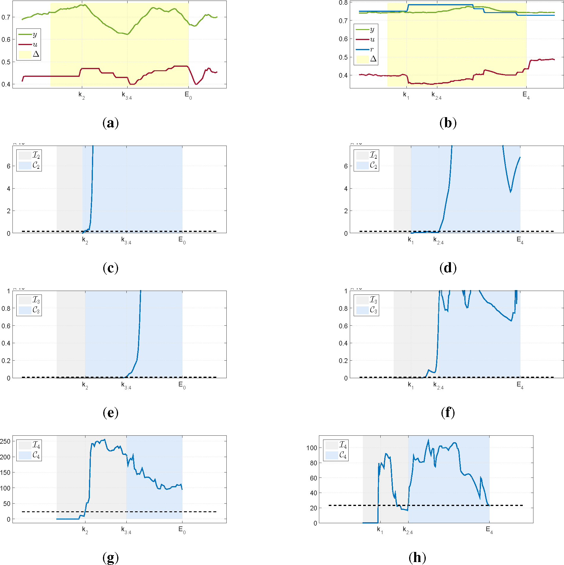The first column in Figure 3 presents one of such intervals retrieved by the algorithm for a level control loop. As can be seen, all quantities respond well to a change in excitation and the retrieved data behaves nicely, with no evident presence of a disturbance.

The second column in Figure 3 presents an interval retrieved from a density loop operating under feedback. As can be noticed, there is a large delay for this plant. A step change is detected at k₁ and, compared to the previous example in Figure 3c, significant changes for the variance of y takes considerably longer time to be detected as seen in Figure 3d. Despite the large delay, the use of a Laguerre expansion can capture the excitation in the data and is well adjusted to the first changes in y. The Granger causality test also indicates the presence of excitation and the algorithm exits when its value returns below the threshold.

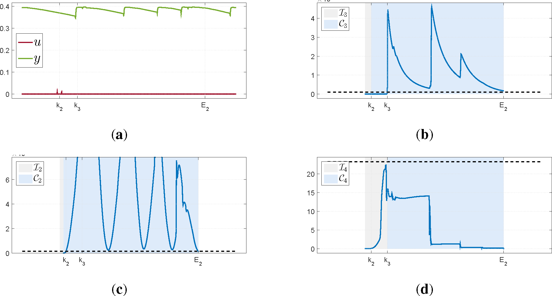
To illustrate the importance of the Granger causality test, we present an example where the interval was rejected because it did not pass this test. The data, seen in Figure 4a, was collected from the open loop operation of a temperature loop. As can be seen, there are almost no changes in u but y is varying considerably due to the presence of an external disturbance. A small change in the input activates the algorithm and because of the disturbances, both the test for the variance of y and the numerical conditioning of $\overline{R}(k)$ exceed the thresholds. However, the Granger causality test remains below the threshold and the interval is not accepted as useful. This example illustrates that the condition number alone is not sufficient to determine the quality of the data.

6. Conclusions

From the quite extensive testing it seems that the method developed in this paper can successfully find intervals of data relevant for system identification. It requires minimal knowledge of the control loops, namely, whether the process is integrating or not. It is implemented efficiently in a recursive manner. A day’s worth of data, from all loops in the test plant, takes less than 10s to be processed.

The developed method is based on classical results from identification theory of linear systems. As an initial screening, it checks that input and output signals are varying at all. Then it forms an information matrix and checks its condition number. Finally, it estimates a provisional model using a Laguerre model structure. If the parameter estimates of this provisional model are found to be statistically non-zero the data interval is marked as potentially useful for system identification and a quality measure is also provided.