Experimental Methodology for Thermo-Mechanical Stress Analysis

Abstract

The experimental analysis of stresses in thermo-mechanical problems is fundamental for the design and evaluation of the mechanical behavior of structures, frames and various machine elements that operate under mechanical and thermal loads. It is also essential for complementing and validating analytical and numerical studies. This paper proposes an experimental methodology that allows the determination of plane states of stress—mechanical, thermal, and thermo-mechanical—based on the experimental measurement of thermo-mechanical deformation states at a surface point. Based on the theory of linear mechanical elasticity and applying the principle of superposition, plane thermo-mechanical constitutive models are developed, and methods are proposed that allow the thermal and mechanical variables in the models to be experimentally decoupled. The methodology was validated by thermal, mechanical and thermo-mechanical tests carried out on test specimens made of three materials: steel, aluminum and brass. The results show effectiveness in decoupling and solving the analytical models corresponding to the plane, mechanical, thermal, and thermo-mechanical states of stress. The maximum deviations obtained between the stresses provided by the formulated models and the experimental results were a maximum of 4% in most cases.

1. Introduction

Experimental stress analysis in thermo-mechanical problems of thermal machinery components and engineering structures is a relevant area in modern engineering. According to Hetnarski and Eslami [1] and Shakeriaski et al. [2], these analyses consider both mechanical stresses, generated by structural loads, and thermal stresses, produced by temperature variations, especially when external or internal constraint limits displacements. Thus, the thermo-mechanical problem can be regarded as a particular case of combined stresses.

The theory of linear elasticity, developed primarily by Dally and Riley [3] and Durelli et al. [4], is widely applied to the study of linear problems involving exclusively mechanical stresses, under the assumptions of infinitesimal strains, homogeneous material, and linear elastic behavior. In the case of thermal stress, the theory of linear thermoelasticity [1,2] and Greene et al. [5] describes the problem assuming constant thermal and mechanical properties under temperature changes.

However, in practice, the coefficient of thermal expansion and elastic constants may vary with temperature. For example, in Poore et al. [6], strain gages were used to experimentally determine the thermal expansion coefficients of various materials over different temperature ranges, observing variations of up to 1.5% in copper under 40 °C changes. In Kiefer et al. [7], an experimental study evaluated the variation in the elastic constants of AISI 4140 steel with increasing temperature, showing that an increase of approximately 400 °C linearly decreases the Young’s modulus by 12%, while Poisson’s ratio increases by 4%. In Ventura et al. [8], thermal contraction phenomena in different materials were analyzed. Likewise, in Montoya et al. [9], a finite element study was developed to analyze fatigue failures in solar receiver tubes, applying thermal loading cycles and evaluating thermal properties as functions of temperature.

It has been shown that the magnitude of thermal stress depends not only on the geometry, temperature change, or the coefficient of thermal expansion and elastic constants, but also on the degree of boundary restraint. In Shabana et al. [10], the absolute nodal coordinate formulation was used to model free thermal expansion—which does not generate stress and restrained thermal expansion—where displacements are limited and thermal stresses are induced.

Thermal stress analysis has important applications in fields such as structural mechanical engineering, electronic systems, and the aerospace industry. For example, structures such as bridges, buildings, and pavements are affected by thermal variations. In Ma et al. [11], strategies are presented to mitigate these effects using reinforcements, expansion joints, insulating coatings, and advanced materials. In the aerospace sector, aircraft and launch vehicle structures operate under extreme temperature and pressure conditions. Also, in Xie et al. [12] and Wan et al. [13], the phenomenon of aero-thermo-elasticity in hypersonic vehicles is studied, considering the coupling of thermal, structural, inertial, and elastic loads, and observing changes in natural frequencies and buckling phenomena. These investigations highlight the need to consider combined effects in structural design. In electronic devices, thermal stresses are a frequent cause of failure, particularly in solder joints, due to differences in thermal expansion coefficients. In Dhumal et al. [14], cooling solutions and thermal design strategies are analyzed to mitigate these effects.

In general, numerous works address thermal stress and thermal fatigue analysis, solving these problems through analytical formulations, numerical simulations, and experimental studies.

Zainuddin et al. [15] addresses the challenges of thermal monitoring in electrical transmission lines exposed to thermal overloads. In Hetnarski and Eslami [1], general formulations for plane strains and stresses in beams, disks, cylinders, and piping systems are presented, while Pitarresi and Patterson [16] describes the general theory of thermoelastic analysis under cyclic or adiabatic loads.

Regarding numerical solutions, in Kayiran H.F. [17], a finite element method (FEM) study analyzed thermal stresses in composite material disks, assuming a constant modulus of elasticity. In Cha and Jin [18], a combined analytical and experimental analysis of thermal stresses in massive concrete structures was carried out using tension and compression tests. In Júnior et al. [19], a numerical model based on the finite difference method was developed to analyze transient thermal stresses in cylinders, validated through strain gage measurements.

Considering thermal fatigue, in Ogunbiyi et al. [20], FEM simulations were performed to evaluate the thermo-mechanical behavior of a steam turbine blade estimating maximum stresses and thermal fatigue life under real operating conditions. Similarly, in Szmytka et al. [21], fatigue failure in pistons subjected to cyclic loads and thermal variations generating alternating stresses is analyzed.

Regarding composite materials, in Delfin et al. [22], an analytical model is proposed to evaluate global and interlaminar thermal stresses in symmetric metal laminates, based on plane thermo-mechanical constitutive models and the principle of superposition. Experimental validation was performed through controlled thermal tests. In Cerracchio et al. [23], the inverse finite element method (iFEM) was used to determine the deformed shape of a reinforced composite panel from experimental data obtained with uniaxial sensors. In Adhe et al. [24], analytical thermoelastic models in nonhomogeneous isotropic strips are studied using iterative techniques.

In general, the thermo-mechanical problem couples displacement fields induced by mechanical and thermal loads. Although a global solution may be sufficient in some cases, for design or structural evaluation purposes, it is necessary to separately identify the strains and stresses induced by each type of load. However, analytical constitutive models usually contain more unknowns than equations, which require decoupling processes. In Thube and Gotkhindi [25], a combined technique between FEM and a complex analytical formulation is proposed, allowing the separation of the global displacement field into structural and thermal components, demonstrating its application in various classical examples.

Experimental thermo-mechanical stress analysis is essential both to validate theoretical models and for the efficient evaluation of mechanical structural elements subjected to thermal and mechanical loads. However, there is no standardized method to experimentally decouple combined thermal and mechanical stresses in a thermo-mechanical problem. Therefore, the main objective of this study is to develop and validate a methodology for the experimental analysis of thermal, mechanical, and thermo-mechanical stresses. To this end, linear analytical constitutive models are developed, and experimental methods are proposed to determine thermal and mechanical stresses integrated into the magnitude of thermo-mechanical stresses. These models were developed by applying the principle of superposition. The methodology is systematic and replicable and, although this study considered a temperature range of 25–40 °C and relatively simple physical models, it can be extended to a wider range of real engineering problems by considering temperature-dependent thermal and mechanical properties.

The methodology developed was validated through controlled thermo-mechanical tests using strain gage rosettes to experimentally determine the plane state of strain at specific points of different physical specimens manufactured from different materials (steel, aluminum, and brass).

2. Materials and Methods

2.1. General Project Methodology

Given that no sufficient linear analytical models are currently available to decouple variables and experimentally analyze plane thermo-mechanical states of stress, this work proposes the development of an analytical model that allows the experimental analysis of mechanical, thermal, and thermo-mechanical states of stress in structural elements.

Notably, the experimental analysis of thermo-mechanical, thermal, and mechanical stress was performed under the plane stress assumption, since measurements were carried out at surface points of the analyzed elements.

The general methodology of the project is as follows:

First, by applying the principle of superposition, since this is a linear problem, and based on the theories of linear elasticity and linear thermos elasticity, a global constitutive model was developed, integrated by particular constitutive models: thermal, mechanical, and thermo-mechanical. Because the developed model presents a greater number of stress unknowns than equations, four cases with different initial conditions were proposed for its solution. For each case, plane constitutive models applicable to a specific point were obtained. Subsequently, by means of the principle of superposition, a global thermo-mechanical constitutive model was integrated, whose solution directly relates the measured strains to the thermal, mechanical, and combined stresses.

To validate this model, simple laboratory specimens were designed and manufactured, on which mechanical, thermal, and thermo-mechanical tests were performed, as shown in Figure 1.

The design of the experimental tests was based on the information derived from the global constitutive model (all involved constitutive models) and on the operating conditions of the real application. Preliminary thermal and/or mechanical tests were defined, as well as thermo-mechanical tests, to obtain measurements that allow for the independent determination of thermal, mechanical, and thermo-mechanical states of stress at the analyzed point via a decoupling process. The decoupling procedure consisted of using the results of the thermal and mechanical tests to calculate characteristic coefficients associated with each type of load and then applying these coefficients to the thermo-mechanical case, considering the contribution of each effect.

Instrumentation was carried out by selecting an appropriate strain gage rosette for the point of interest and establishing a reference coordinate system consistent with the geometry and loading state. To eliminate the influence of free thermal expansion on the measurements, it is suggested to additionally instrument a point on an alternate element made of the same material, connected in a half Wheatstone bridge, which is subjected exclusively to free thermal expansion.

Finally, the experimental tests performed were:

• Thermal test, to determine a linear coefficient associated with thermal loads.
• Mechanical test, aimed at determining a coefficient related to structural or mechanical loads.
• Thermo-mechanical test, aimed at obtaining the state of strain at the point under the simultaneous action of thermal and mechanical loads.

In all cases, boundary restraints and mechanical loads were applied at the same points of the fabricated physical models.

From the strains recorded by the rosette elements, the state of strain at the point was determined, with components referred to the established coordinate system. With these results and applying the thermo-mechanical constitutive models, the thermal, mechanical, and thermo-mechanical states of stress were calculated. In the thermal and thermo-mechanical cases, a free thermal expansion test was performed separately and subtracted from the measured values, which is equivalent to connecting each strain component, in a half Wheatstone bridge, with a dummy element to ensure thermal compensation and measurement accuracy.

2.2. Analytical Models

The linear thermoelastic constitutive models proposed in this article are based on the linear theories of elasticity and thermos-elasticity, as well as on the principle of superposition [3]. The main objective is to determine the global plane thermo-mechanical states of stress, as well as the plane thermal and mechanical states of stress at a structural point.

The assumptions of the thermo-mechanical problem are as follows:

• The materials of the structures are linear elastic, homogeneous, and isotropic.
• The problems are within the range of infinitesimal strains.
• The developed thermo-mechanical analytical models are linear.
• The principles used correspond to linear elasticity and linear thermos-elasticity theory.
• The temperature range in the experimental tests is between 10 °C and 100 °C.
• The problems satisfy geometric linearity.

The analytical models for experimental analysis correspond to surface points of the structures, that is, points with plane states of stress.

2.2.1. Mechanical Model

The mechanical constitutive models are as follows:

State of strain as a linear function of the state of stress:

$${\epsilon }_{xM}= {\displaystyle \frac{1}{E}}\left[{\sigma }_{xM}-{\nu \sigma }_{yM}\right]$$

(1a)

$${\epsilon }_{yM}={\displaystyle \frac{1}{E}}\left[{\sigma }_{yM}-{\nu \sigma }_{xM}\right]$$

(1b)

$${\gamma }_{xyM}={\displaystyle \frac{{\tau }_{xyM}}{G}}$$

(1c)

State of stress as a linear function of the state of strain:

$${\sigma }_{xM}={\displaystyle \frac{E{\epsilon }_{xM}}{\left(1-{\nu }^2\right)}}+{\displaystyle \frac{\nu E{\epsilon }_{yM}}{\left(1-{\nu }^2\right)}}$$

(2a)

$${\sigma }_{yM}={\displaystyle \frac{\nu E{\epsilon }_{xM}}{\left(1-{\nu }^2\right)}}+{\displaystyle \frac{E{\epsilon }_{yM}}{\left(1-{\nu }^2\right)}}$$

(2b)

$${\tau }_{xyM}={\gamma }_{xyM}G$$

(2c)

where E and ν are the Young’s modulus and Poisson’s ratio, respectively. Likewise, ${\sigma }_{xM}$, ${\sigma }_{yM}$ and ${\tau }_{xyM}$ are the normal and shear mechanical stress components with respect to an x–y coordinate system, while ${\epsilon }_{xM}$, ${\epsilon }_{yM}$ and ${\gamma }_{xyM}$ define the plane state of strain at the point.

2.2.2. Thermal Model

The thermal constitutive model is a state of strain as a linear function of the state of stress:

$${\epsilon }_{xT}= {\displaystyle \frac{1}{E}}\left[{\sigma }_{xT}-{\nu \sigma }_{yT}\right]+\Delta T\alpha$$

(3a)

$${\epsilon }_{yT}={\displaystyle \frac{1}{E}}\left[{\sigma }_{yT}-{\nu \sigma }_{xT}\right]+\Delta T\alpha$$

(3b)

$${\gamma }_{xyT}={\displaystyle \frac{{\tau }_{xyT}}{G}}$$

(3c)

Considering free thermal expansion:

$${\epsilon }_{xFT}=\alpha \Delta T,{ \epsilon }_{yFT}=\alpha \Delta T,{\gamma }_{xyFT}=0$$

(4)

The previous equations, in terms of strains, can be written as:

$${\epsilon }_{xT}={\epsilon }_{xT}+{\epsilon }_{xFT}$$

(5a)

$${\epsilon }_{xT}={\epsilon }_{xT}+{\epsilon }_{xFT}$$

(5b)

$${\gamma }_{xyFT}=0$$

(5c)

State of stress as a linear function of the state of strain:

$${\sigma }_{xT}={\displaystyle \frac{E}{1-{\nu }^2}}{\epsilon }_{xT}+{\displaystyle \frac{\nu E}{1-{\nu }^2}}{\epsilon }_{yT}$$

(6a)

$${\sigma }_{yT}={\displaystyle \frac{\nu E}{1-{\nu }^2}}{\epsilon }_{xT}+{\displaystyle \frac{E}{1-{\nu }^2}}{\epsilon }_{yT}$$

(6b)

$${\tau }_{xyT}=G{\gamma }_{xyT}$$

(6c)

where ${\epsilon }_{xFT}$ and ${\epsilon }_{yFT}$ are the thermal strains due to free expansion, while ${\epsilon }_{xT}$, ${\epsilon }_{yT}$ and ${\gamma }_{xyT}$ are the thermal strains caused by thermal stresses. Thus, ${\sigma }_{xT}$, ${\sigma }_{yT}$ and ${\tau }_{xyT}$ correspond to the plane thermal normal and shear stresses.

2.2.3. Thermo-Mechanical Model

The thermo-mechanical problem is assumed to be linear, and within the operating temperature range, the elastic and thermal constants of the mechanical system and the constraint system are considered constant. Furthermore, the problem satisfies:

• Geometric linearity.
• The linear effect of structural constraints, for any temperature within the working range and for any applied mechanical load.
• Temperature gradients with controlled variation at all stages of the problem.
• External loads that may change in magnitude, but whose position vector remains constant.

If these considerations are satisfied, it is possible to apply the principle of superposition. Thus, the global thermo-mechanical problem can be represented as the sum of the individual mechanical and thermal problems:

$${\sigma }_{xTM}={\sigma }_{xM}+{\sigma }_{xT}$$

(7a)

$${\sigma }_{yTM}={\sigma }_{yM}+{\sigma }_{yT}$$

(7b)

$${\tau }_{xyTM}={\tau }_{xyM}+{\tau }_{xyT}$$

(7c)

where

$${\sigma }_{xTM}={\displaystyle \frac{E}{1-{\nu }^2}}{\epsilon }_{xTM}+{\displaystyle \frac{\nu E}{1-{\nu }^2}}{\epsilon }_{yTM}$$

(8a)

$${\sigma }_{yTM}={\displaystyle \frac{\nu E}{1-{\nu }^2}}{\epsilon }_{xTM}+{\displaystyle \frac{E}{1-{\nu }^2}}{\epsilon }_{yTM}$$

(8b)

$${\tau }_{xyTM}=G{\gamma }_{xyTM}$$

(8c)

Likewise:

$${\epsilon }_{xTM}={\epsilon }_{xT}+{\epsilon }_{xM}$$

(9a)

$${\epsilon }_{yTM}={\epsilon }_{yT}+{\epsilon }_{yM}$$

(9b)

$${\gamma }_{xyTM}={\gamma }_{xyT}+{\gamma }_{xyM}$$

(9c)

And:

$${\epsilon }_{xTM}={\displaystyle \frac{1}{E}}({\sigma }_{xTM}-\nu {\sigma }_{yTM})+\alpha \Delta T$$

(10a)

$${\epsilon }_{yTM}={\displaystyle \frac{1}{E}}({\sigma }_{yTM}-\nu {\sigma }_{xTM})+\alpha \Delta T$$

(10b)

$${\gamma }_{xyTM}={\displaystyle \frac{{\tau }_{xyTM}}{G}}$$

(10c)

where ${\epsilon }_{xTM}$, ${\epsilon }_{yTM}$ and ${\gamma }_{xyTM}$ are the thermo-mechanical strains, and ${\sigma }_{xTM}$, ${\sigma }_{yTM}$ and ${\tau }_{xyTM}$ are the thermo-mechanical stresses.

2.2.4. Correlation Coefficients

Correlation coefficients are defined for mechanical and thermal strains. Considering that the thermal and mechanical problems are linear, for different magnitudes of external loads and different temperature ranges, then:

$$K_{iT}={\displaystyle \frac{\Delta {\epsilon }_{ijT}}{\Delta T_i}}$$

(11)

$$K_{iM}={\displaystyle \frac{\Delta {\epsilon }_{ijM}}{\Delta P_i}}$$

(12)

where $\Delta {\epsilon }_{ijT}$, $\Delta {\epsilon }_{ijM}$, $\Delta T_i$ and $\Delta P_i$ are the respective changes in strains, temperatures, and mechanical loads, and $K_{iT}$ and $K_{iM}$ are the correlation coefficients between strain changes and thermal and mechanical load changes, respectively.

These coefficients correspond to the thermal or mechanical strain of each of the three elements of the strain gage rosette (with i = A, B, C). The subscripts i and j of the strains correspond to the x or y directions. The coefficients are useful when it is required to determine the strain term for a specific value of P and T within the temperature and load ranges considered for obtaining $K_{iT}$ and $K_{iM}$.

2.3. Decoupling of Variables

The analytical constitutive models for the thermo-mechanical problem are coupled with respect to strain components: free thermal strains, restrained thermal strains (which generate thermal stresses), mechanical strains, and thermo-mechanical strains. Decoupling and solution of the system are possible if:

(a) Under the assumption that the considered problems are linear, the principle of superposition is applied, that is:

$${\epsilon }_{xTM}={\epsilon }_{xM}+{\epsilon }_{xT}$$

(13a)

$${\epsilon }_{yTM}={\epsilon }_{yM}+{\epsilon }_{yT}$$

(13b)

$${\gamma }_{xyTM}={\gamma }_{xyM}+{\gamma }_{xyT}$$

(13c)

(b) It is possible to perform preliminary tests to determine the coefficients K_iT and K_iM.

2.3.1. Determination of the Coefficients $K_{iT}$ and $K_{iM}$

The coefficients $K_{iT}$ and $K_{iM}$ are obtained for each rosette element by performing experimental tests, applying mechanical loads and thermal loads with restrained boundaries, respectively. It should be noted that these coefficients are specific to the analyzed problem, since boundary conditions cannot necessarily be reproduced identically.

Determination of $K_{iM}$

A preliminary mechanical test is carried out, without applying the working temperature or before placing the specimen in the thermal incubator. This test is performed at a constant temperature, ambient or different, but within the working range. For greater accuracy, several tests with different load magnitudes are recommended; however, a single test at the actual operating load magnitude may also be performed.

In all cases, the system is initially calibrated to zero and, for each applied mechanical load, the strains provided by each rosette element are recorded. With the load and strain values, the results are plotted and the slopes are determined, which correspond to the coefficients $K_{iM}$.

Determination of $K_{iT}$

A preliminary thermal test is carried out (without mechanical load or with constant mechanical load), calibrating the data acquisition system to zero. Boundary conditions were constrained, and temperatures were gradually increased. Strains are recorded for several temperature values, ensuring that the temperature is stable and homogenized in the analysis zone or element. With the temperature and strain values for each rosette element, the results are plotted and the slopes $K_{iT}$ are determined. In this work, temperature readings were taken every 3 °C within the interval of 25–40 °C, allowing sufficient time for thermal stabilization at each measurement point. Additionally, it is recommended to evaluate the degree of linearity of the thermo-mechanical response.

2.3.2. Analytical Models for Thermal (T), Mechanical (M), and Thermo-Mechanical (TM) Stress Analysis

Although the constitutive expressions share the same mathematical structure, they are presented explicitly for each case to define independent analytical models associated with different available input conditions.

CASE I: With M and T Information

Once the coefficients $K_{iT}$ and $K_{iM}$ are determined, and the working temperature and load are known, from Equations (1a–c)–(3), (4)–(6) and (13), the M-T analytical model is obtained to determine the TM, M, and T states of stress:

$${\sigma }_{xT}={\displaystyle \frac{E{\epsilon }_{xT}+E\nu {\epsilon }_{yT}}{1-{\nu }^2}},{\sigma }_{yT}={\displaystyle \frac{E\nu {\epsilon }_{xT}+E{\epsilon }_{yT}}{1-{\nu }^2}}$$

(14a)

$${\tau }_{xyT}=G{\gamma }_{xyT}$$

(14b)

$${\sigma }_{xM}={\displaystyle \frac{E{\epsilon }_{xM}+E\nu {\epsilon }_{yM}}{1-{\nu }^2}},{\sigma }_{yM}={\displaystyle \frac{E\nu {\epsilon }_{xM}+E{\epsilon }_{yM}}{1-{\nu }^2}}$$

(14c)

$${\tau }_{xyM}=G{\gamma }_{xyM}$$

(14d)

$${\sigma }_{xTM}={\displaystyle \frac{E(\nu {\epsilon }_{yM}+\nu {\epsilon }_{yT}+{\epsilon }_{xM}+{\epsilon }_{xT})}{1-{\nu }^2}}$$

(14e)

$${\sigma }_{yTM}={\displaystyle \frac{E(\nu {\epsilon }_{xM}+\nu {\epsilon }_{xT}+{\epsilon }_{yM}+{\epsilon }_{yT})}{1-{\nu }^2}}$$

(14f)

$${\tau }_{xyTM}=G({\gamma }_{xyM}+{\gamma }_{xyT})$$

(14g)

CASE II: With T and TM Information

The mechanical load P is unknown, but the thermal strains, working temperatures, or coefficient $K_{iT}$, as well as the thermo-mechanical state of strain, are known. In this case, the TM, M, and T states of stress are determined using the T–TM model, Equations (1)–(3), (7)–(10) and (13):

$${\sigma }_{xT}={\displaystyle \frac{E{\epsilon }_{xT}+E\nu {\epsilon }_{yT}}{1-{\nu }^2}},{\sigma }_{yT}={\displaystyle \frac{E\nu {\epsilon }_{xT}+E{\epsilon }_{yT}}{1-{\nu }^2}}$$

(15a)

$${\tau }_{xyT}=G{\gamma }_{xyT}$$

(15b)

$${\sigma }_{xTM}={\displaystyle \frac{E{\epsilon }_{xTM}+E\nu {\epsilon }_{yTM}}{1-{\nu }^2}},{\sigma }_{yTM}={\displaystyle \frac{E\nu {\epsilon }_{xTM}+E{\epsilon }_{yTM}}{1-{\nu }^2}}$$

(15c)

$${\tau }_{xyTM}=G{\gamma }_{xyTM}$$

(15d)

$${\sigma }_{xM}={\displaystyle \frac{E(\nu {\epsilon }_{yTM}-\nu {\epsilon }_{yT}+{\epsilon }_{xTM}-{\epsilon }_{xT})}{1-{\nu }^2}}$$

(15e)

$${\sigma }_{yM}={\displaystyle \frac{E(\nu {\epsilon }_{xTM}-\nu {\epsilon }_{xT}+{\epsilon }_{yTM}-{\epsilon }_{yT})}{1-{\nu }^2}}$$

(15f)

$${\tau }_{xyM}=G({\gamma }_{xyTM}-{\gamma }_{xyT})$$

(15g)

CASE III: With M and TM Information

The temperature T is unknown, but $K_{iM}$, the working load, and the thermo-mechanical state of strain are known. In this case, the TM, M, and T states of stress are determined using the M–TM model, Equations (4)–(10) and (13):

$${\sigma }_{xM}={\displaystyle \frac{E{\epsilon }_{xM}+E\nu {\epsilon }_{yM}}{1-{\nu }^2}}, {\sigma }_{yM}={\displaystyle \frac{E\nu {\epsilon }_{xM}+E{\epsilon }_{yM}}{1-{\nu }^2}}$$

(16a)

$${\tau }_{xyM}=G{\gamma }_{xyM}$$

(16b)

$${\sigma }_{xTM}={\displaystyle \frac{E{\epsilon }_{xTM}+E\nu {\epsilon }_{yTM}}{1-{\nu }^2}},{ \sigma }_{yTM}={\displaystyle \frac{E\nu {\epsilon }_{xTM}+E{\epsilon }_{yTM}}{1-{\nu }^2}}$$

(16c)

$${\tau }_{xyTM}=G{\gamma }_{xyTM}$$

(16d)

$${\sigma }_{xT}={\displaystyle \frac{E(\nu {\epsilon }_{yTM}-\nu {\epsilon }_{yM}+{\epsilon }_{xTM}-{\epsilon }_{xM})}{1-{\nu }^2}}$$

(16e)

$${\sigma }_{yT}={\displaystyle \frac{E(\nu {\epsilon }_{xTM}-\nu {\epsilon }_{xM}+{\epsilon }_{yTM}-{\epsilon }_{yM})}{1-{\nu }^2}}$$

(16f)

$${\tau }_{xyT}=G({\gamma }_{xyTM}-{\gamma }_{xyM})$$

(16g)

CASE IV: With Only the Thermo-Mechanical State of Strain

The loads P and T are unknown, as well as the coefficients $K_{iT}$ and $K_{iM}$, but the thermo-mechanical state of strain is known. In this case, only the global thermo-mechanical state of stress can be determined:

$${\sigma }_{xTM}={\displaystyle \frac{E{\epsilon }_{xTM}+E\nu {\epsilon }_{yTM}}{1-{\nu }^2}},{ \sigma }_{yTM}={\displaystyle \frac{E\nu {\epsilon }_{xTM}+E{\epsilon }_{yTM}}{1-{\nu }^2}}$$

(17a)

$${\tau }_{xyTM}=G{\gamma }_{xyTM}$$

(17b)

If none of the previous cases can be applied, it is not possible to decouple the system, and only the global thermo-mechanical stresses can be obtained.

2.4. Experimental Design

The development of the experimental tests for the application and evaluation of the proposed methodology, applying analytical models, Equations (14)–(17), depends on: (a) the real conditions of the considered problem (working temperatures and mechanical loads, materials, and boundary restraints), (b) the geometry and material of the specimens, and (c) the assumptions and principles of the applied experimental technique.

2.4.1. Design and Fabrication of Specimens

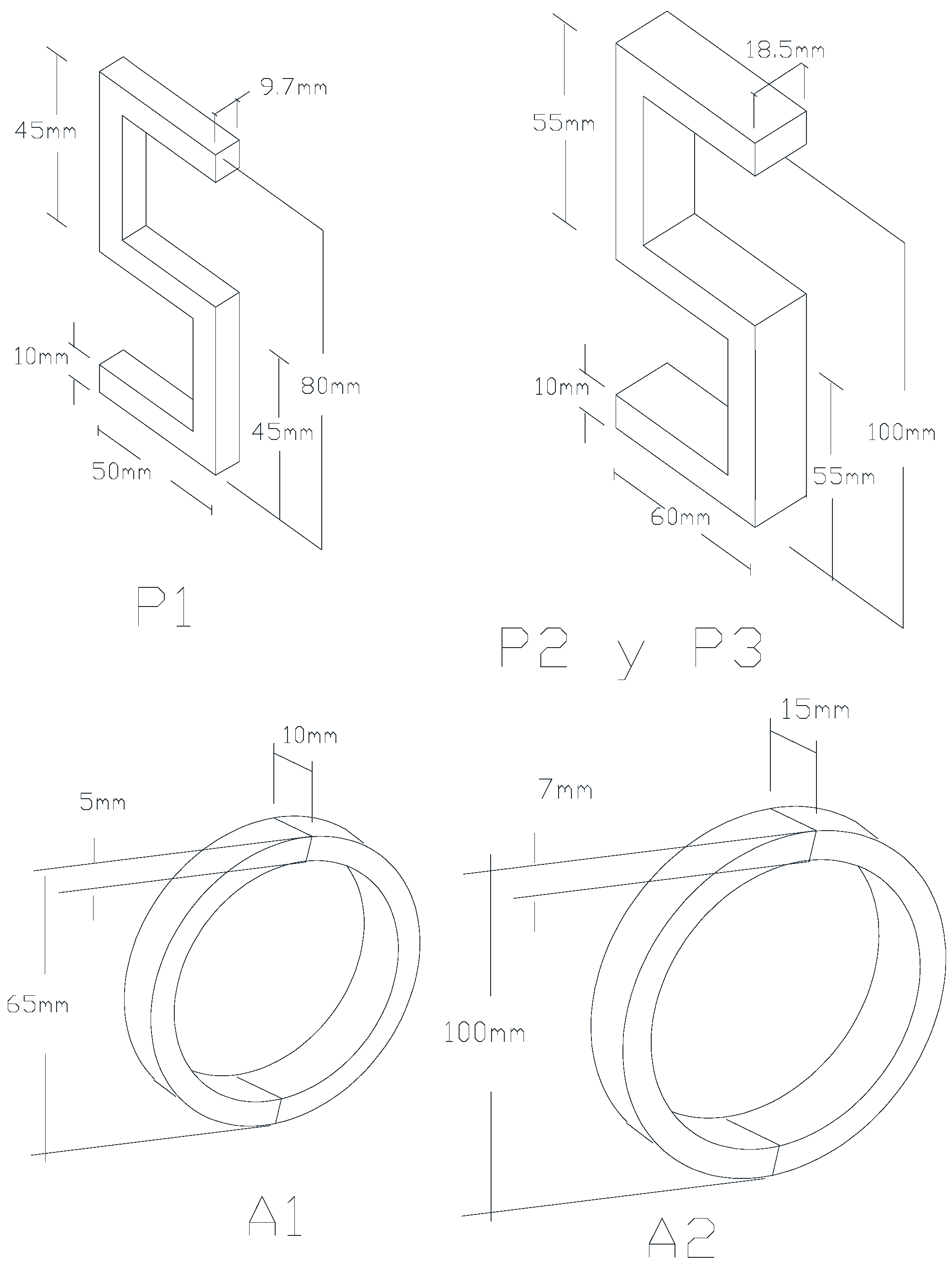
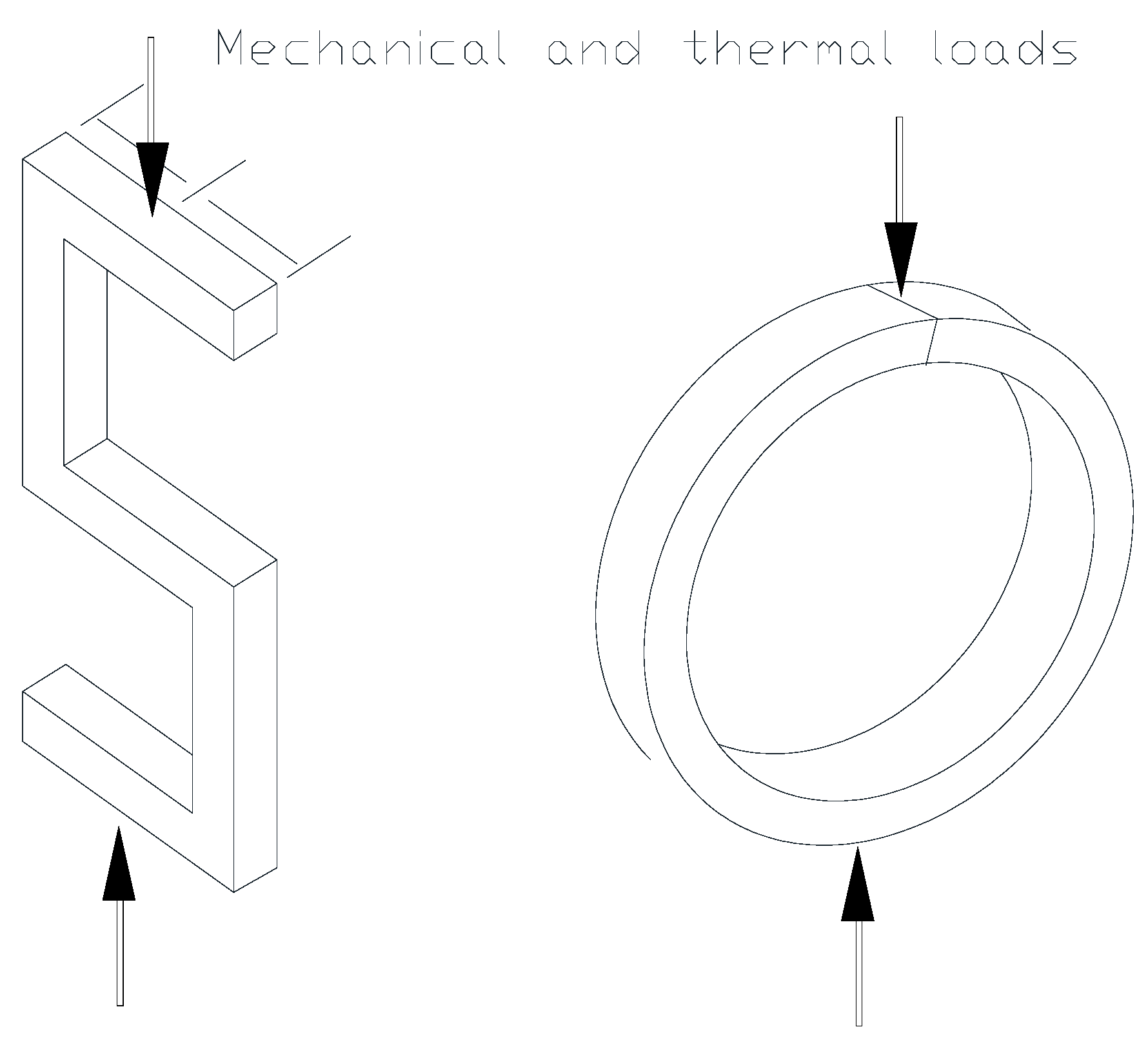
For the experimental tests, specimens with simple geometries, both rectangular and annular, were designed and manufactured using a mechanical milling machine. The specimens and their main dimensions are shown in Figure 1. The rectangular specimens were labeled P1, P2, and P3, while the annular specimens were identified as A1 and A2. The material of each specimen is presented in

Table 1. Labels of physical models.

Physical Models	Material
A1	Brass
A2	Aluminum
P1	Steel
P2	Aluminum
P3	Steel

. Figure 2 shows the boundary restraints, which correspond to the points where the thermal and mechanical loads were applied for each geometric configuration (models A and P).

2.4.2. Design of Experimental Tests

Considering the analytical models corresponding to Cases I–IV, the specimens, and the thermal and mechanical characteristics of the thermo-mechanical problem, the necessary preliminary thermal and/or mechanical tests, as well as the actual thermo-mechanical tests, were defined. This allows selecting the points to be instrumented, determining the thermo-mechanical state of stress at a point, and solving the corresponding analytical model for the thermo-mechanical, thermal, and mechanical states of stress.

The experimental tests have one of the following objectives:

(I)

To determine only the thermo-mechanical state of stress, in which case performing the general thermo-mechanical test is sufficient.

(II)

To determine the thermal and mechanical states of stress in addition to the thermo-mechanical state.

2.4.3. Instrumentation

For the experimental stress analysis, the electrical resistance strain gage technique was used, following this procedure:

• Based on the geometry of the structural element, its restraints, and its thermal and mechanical loads, the point or points of interest at which the plane state of stress is to be determined, were selected. In this work, these points were selected considering that the stress level at that position is relevant.
• The type of rosette suitable for the specimen dimensions and test conditions was selected, namely the EA-13-060RZ-120/E rosette from micro-measurements [26].
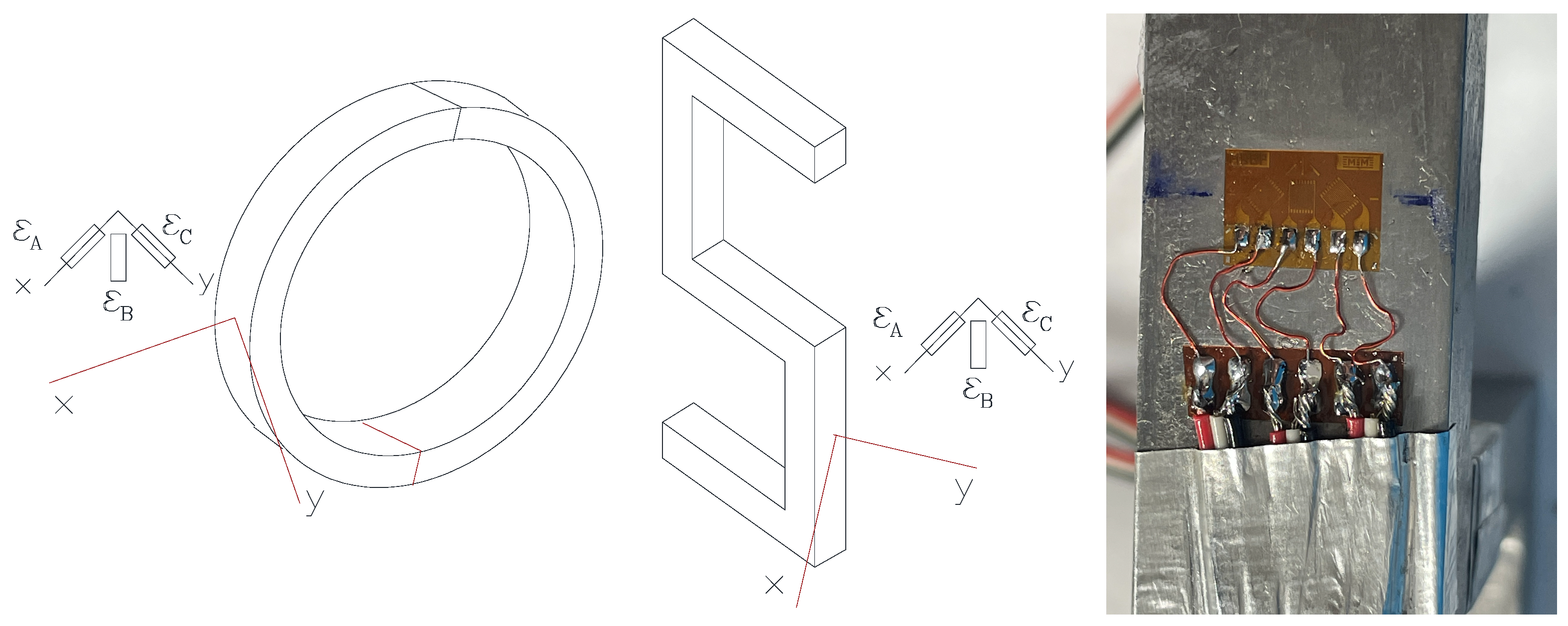
• At the selected point or points, the reference coordinate system was established, and the rosette was installed (Figure 3).

It is recommended to instrument, using the same type of rosette, a point on a dummy specimen made of the same material [27], which should be placed in a location that ensures it reaches the same temperature as the instrumented point of the structure. This allows, by connecting each rosette element with one of these dummy elements in a half Wheatstone bridge, eliminating thermal effects due to free expansion. The reason is that this dummy element will be subjected only to free thermal expansion and, when connected in a half bridge, will eliminate the free thermal expansion of the mechanical structure. Likewise, this makes it unnecessary to use the coefficients of thermal expansion of the materials, which reduces uncertainties in the test.

In this work, due to the relevance of the study, the mentioned elimination was carried out by performing free thermal expansion tests at the same temperatures as the thermal tests with restrained specimens. The obtained data were subtracted from those obtained in the restrained thermal test.

2.4.4. Experimental Tests

The experimental tests are defined according to the real problem situation and the possible tests to be performed. The evaluation tests in this work are as follows:

• Free thermal expansion test (FT)
• Thermal test (T)
• Mechanical test (M)
• Thermo-mechanical tests (TM)

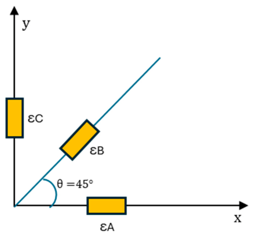
During the tests, the strains provided by each rosette element (A, B, and C) were recorded using a Strain Indicator P3, strains ${\epsilon }_A$, ${\epsilon }_B$ and ${\epsilon }_C$. Subsequently, using Equation (A2) of Appendix A [3], the plane state of strain ${\epsilon }_x$, ${\epsilon }_x$ and ${\gamma }_{xy}$, with respect to the x–y axes, was determined.

The P3 Strain Indicator and Recorder is a portable precision instrument. It supports 120, 350, and 1000 ohm strain gages and allows full-, half-, and quarter-bridge configurations. The measurement range is ±31,000 µε, with a resolution of ±1 µε. The applicable temperature range depends on the selected strain gage.

The free thermal expansion, thermal, and thermo-mechanical tests were denoted with the suffixes FT, T, and TM, respectively, and are described below:

FT tests (free expansion):

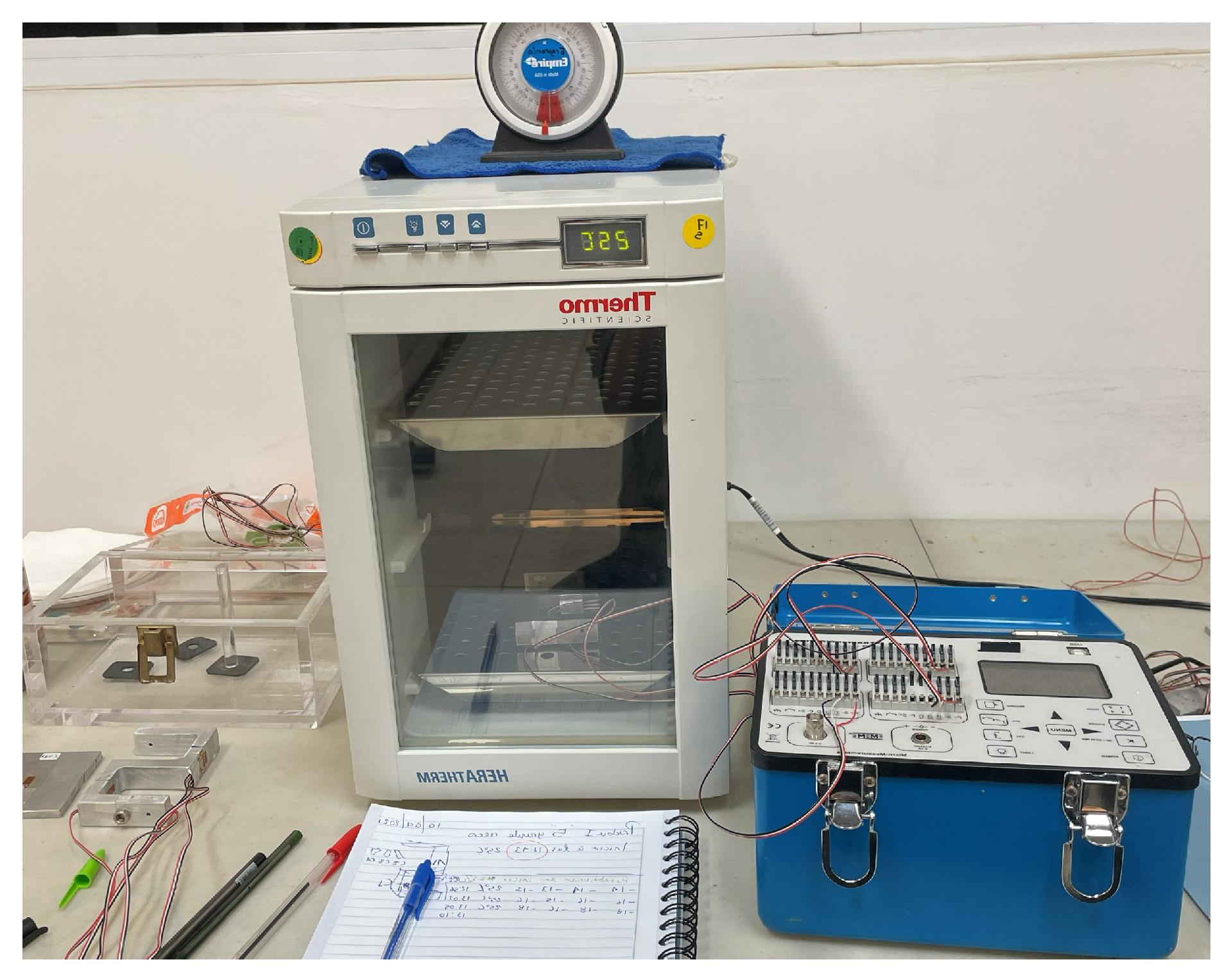
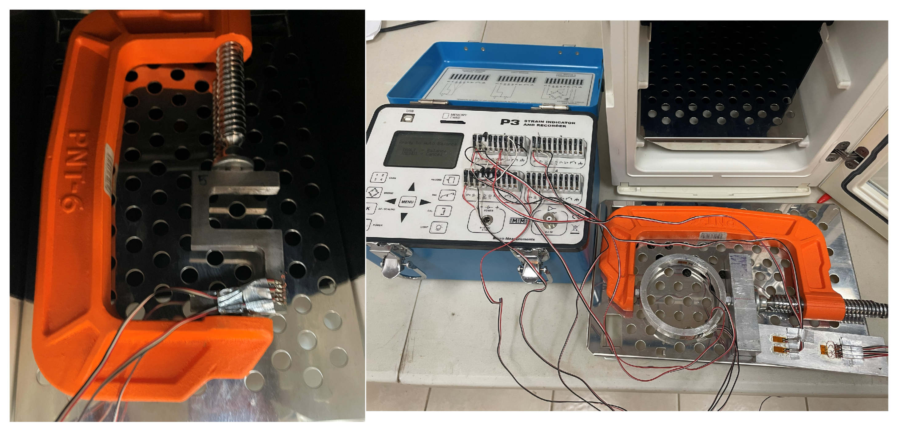
Each specimen (P1–P3, A1, and A2) was subjected to free expansion, that is, temperature changes without boundary restraints. Each instrumented specimen was placed in a Thermo Scientific incubator and brought to a temperature of 25 °C, calibrating the strain indicator to zero (Figure 4). Temperature increments of 3 °C up to 40 °C were applied, waiting with a stabilization time between 30 and 60 min, depending on the specimen, the material and the stabilization of the strains in the rosette elements.

T tests for the determination of coefficients $K_{iT}$:

To reproduce thermal stress caused by boundary restraints and temperature changes, the specimens with their restraints were placed inside the incubator, as shown in Figure 5, and the system was calibrated at 25 °C as the initial or reference value. The temperature gradually increased by 3 °C to 40 °C, waiting with a stabilization time between 30 and 60 min, taking strain readings from the rosette elements. When dummy elements are used, the strains obtained at the indicator correspond directly to thermal loads. In the present work, since dummy elements were not used, the values obtained in the FT tests were subtracted from those obtained in the restrained thermal test. The final results were plotted and the coefficient $K_{iT}$ was determined for each specimen.

M tests for the determination of coefficients $K_{iM}$:

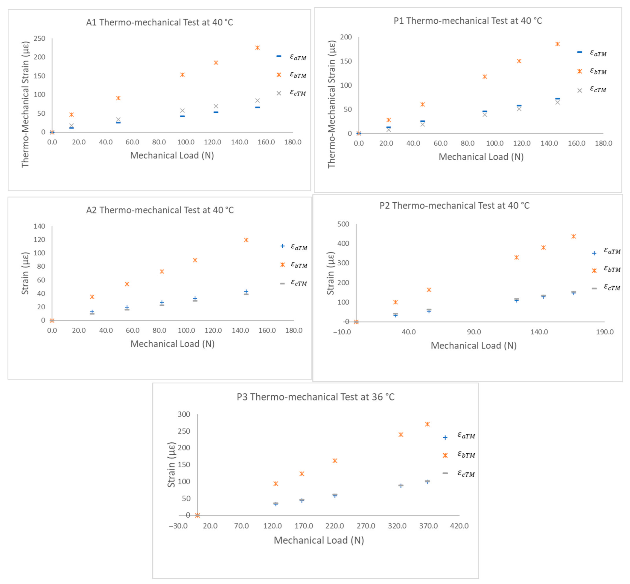
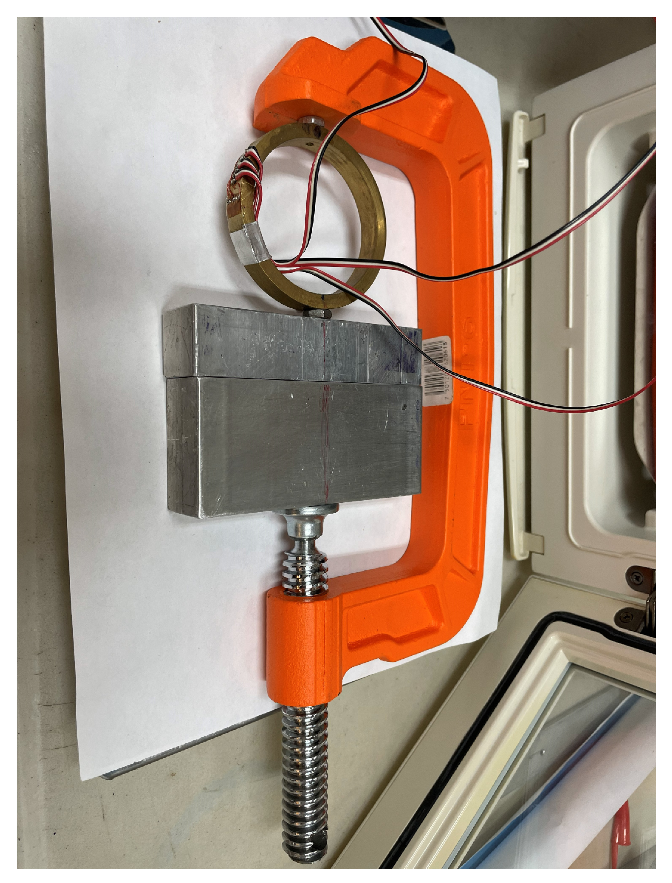
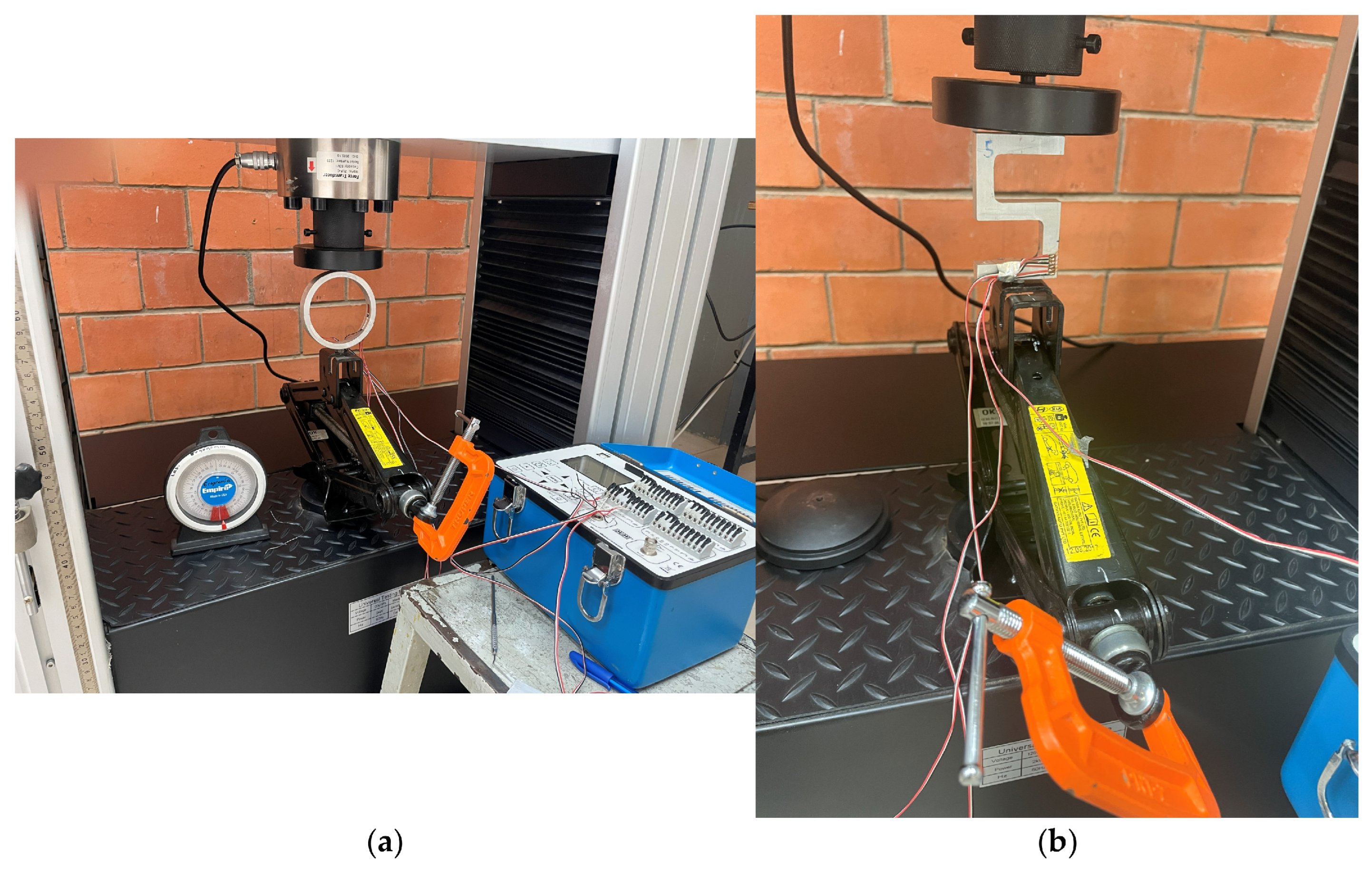
Various compressive loads (0–370 N) were applied to each specimen at a constant ambient temperature of 19 °C using a C-type press, as shown in Figure 6. The selected load range was sufficient to generate measurable strain signals in the rosette elements. The loads were applied slowly under quasi-static conditions to avoid disturbing the restraint configuration and to ensure stable strain measurements. The mechanical loads were compressive at the restraint points, as shown in Figure 6. The magnitude of the loads was obtained by calibrating each specimen as a load cell, utilizing the instrumented rosettes (Figure 7). Figures in Appendix D show the load versus strain results of the B element of the rosette and their respective linear calibration functions for each specimen (A1, A2, P1, P2, and P3). The load range in the mechanical tests was selected based on the information obtained during the calibration of the specimens as load cells.

TM tests for the determination of the state of strain and the thermo-mechanical state of stress:

At a working temperature higher than the initial or reference temperature (40 °C to models A1, A2, P1 and P2, and 36 °C to model P3), with thermal loads present and various mechanical working loads applied, strain readings were taken. If dummy elements had been used, the readings would correspond directly to thermo-mechanical strains. In the tests of this work, the values obtained in the FT tests at the same temperature were subtracted from the resulting readings. For evaluation, at the working temperature, various loads were applied using the “C” type press, producing different thermo-mechanical states of strain.

The strain acquisition system (Strain Indicator P3) was calibrated to zero before each test.

2.5. Experimental Stress Analysis

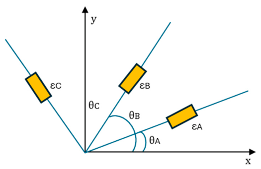
For each condition (Cases I–IV) and with the strains provided by the rosette elements (${\epsilon }_A$, ${\epsilon }_B$ and ${\epsilon }_C$), the plane states of strain at the point or points, ${\epsilon }_x$, ${\epsilon }_x$ and ${\gamma }_{xy}$, were determined using Equations (A1) and (A2) in Appendix A, referred to the established axes (Figure A1 and Figure A2).

With these strain states and the corresponding constitutive models, depending on the type of case (analytical models of Equations (14)–(17)), the thermal, mechanical, and thermo-mechanical states of stress were calculated.

3. Results

3.1. Results of the Experimental Thermomechanical

The results of the experimental analysis of thermal (T), mechanical (M), and thermo-mechanical (TM) stresses are presented and are the results of the individual tests FT, T, M, and TM and the possible cases (I–IV). Each experimental test was carried out on each specimen (P1, P2, P3, A1 and A2). Results are considered for two conditions: for each of the temperatures established during the controlled tests and for a specific case at a given temperature and mechanical load, namely T–M, T–TM, and M–TM.

3.1.1. Individual Experimental Thermo-Mechanical Testing

To evaluate the functionality of the methodology for Cases I–IV, each of the five specimens P1, P2, P3, A1 and A2 was subjected to the individual experimental thermo-mechanical tests FT, T, M, and TM.

The FT and T tests were carried out under controlled experiments, establishing 25 °C as the reference temperature, calibrating the initial strain gage readings to zero, and considering 25 °C as the initial temperature of the test. Strain readings provided by each rosette element were taken every 3 °C up to 40 °C. The T test was conducted with the boundary restraints shown in Figure 5 and Figure 6.

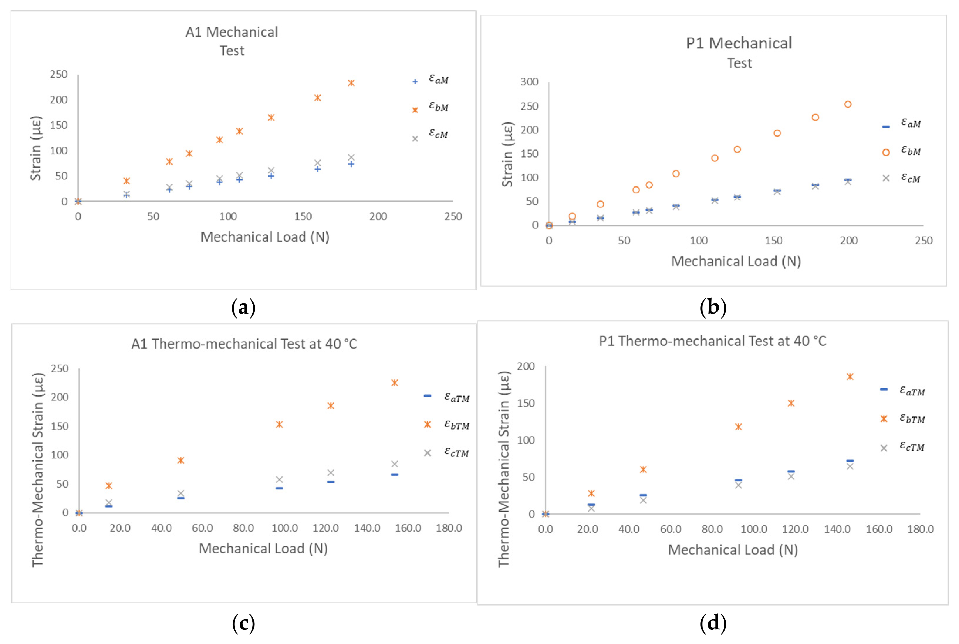
All results are presented in the graphs in Figure 8 and in Appendix B, for T, M and TM, and the results for FT are included in Table 2, Table 3 and Table 4 and Appendix C.

3.1.2. T–M, T–TM, and M–TM Solutions

Table 2, Table 3, Table 4,

Table A1. Determination of stresses TM, P1 model at 40 °C.

	Separate State of Strain									Calculate State of Stress									Thermo-Mechanical Experimental Stress Analysis (Mpa)
	Thermal State of Strain (με)			Mechanical State of Strain (με)			Thermo-Mechanical State of Strain (με)			Mechanical State of Stress (Mpa)			Thermal State of Stress (Mpa)			Thermo-Mechanical State of Stress (Mpa)
Mechanical Load (N)	${\mathit{\epsilon }}_{\mathit{x}\mathit{T}}$	${\mathit{\epsilon }}_{\mathit{y}\mathit{T}}$	${\mathit{\gamma }}_{\mathit{x}\mathit{y}\mathit{T}}$	${\mathit{\epsilon }}_{\mathit{x}\mathit{M}}$	${\mathit{\epsilon }}_{\mathit{y}\mathit{M}}$	${\mathit{\gamma }}_{\mathit{x}\mathit{y}\mathit{M}}$	${\mathit{\epsilon }}_{\mathit{x}\mathit{T}\mathit{M}}$	${\mathit{\epsilon }}_{\mathit{y}\mathit{T}\mathit{M}}$	${\mathit{\gamma }}_{\mathit{x}\mathit{y}\mathit{T}\mathit{M}}$	${\mathit{\sigma }}_{\mathit{x}\mathit{M}}$	${\mathit{\sigma }}_{\mathit{y}\mathit{M}}$	${\mathit{\tau }}_{\mathit{x}\mathit{y}\mathit{M}}$	${\mathit{\sigma }}_{\mathit{x}\mathit{T}}$	${\mathit{\sigma }}_{\mathit{y}\mathit{T}}$	${\mathit{\tau }}_{\mathit{x}\mathit{y}\mathit{T}}$	${\mathit{\sigma }}_{\mathit{x}\mathit{T}\mathit{M}}$	${\mathit{\sigma }}_{\mathit{y}\mathit{T}\mathit{M}}$	${\mathit{\tau }}_{\mathit{x}\mathit{y}\mathit{T}\mathit{M}}$	${\mathit{\sigma }}_{\mathit{x}\mathit{T}\mathit{M}\mathit{R}}$	${\mathit{\sigma }}_{\mathit{y}\mathit{T}\mathit{M}\mathit{R}}$	${\mathit{\tau }}_{\mathit{x}\mathit{y}\mathit{T}\mathit{M}\mathit{R}}$
0.00	0	$-1$	1	0	0	0	0	0	0	0.00	0.00	0.00	0.00	0.00	0.00	0.00	0.00	0.00	0.00	0.00	0.00
21.93	0	$-1$	1	12	8	36	13	8	35	3.13	2.51	2.79	$-0.06$	$-0.22$	0.08	3.06	2.29	2.87	3.35	2.57	2.71
47.09	0	$-1$	1	24	19	77	25	19	76	6.44	5.67	5.97	$-0.06$	$-0.22$	0.08	6.38	5.45	6.05	6.66	5.73	5.89
92.70	0	$-1$	1	45	39	152	46	39	151	12.30	11.37	11.78	$-0.06$	$-0.22$	0.08	12.23	11.15	11.86	12.51	11.43	11.71
117.87	0	$-1$	1	57	51	192	58	51	191	15.68	14.75	14.88	$-0.06$	$-0.22$	0.08	15.61	14.53	14.96	15.89	14.81	14.81
146.18	0	$-1$	1	71	64.5	236.5	72	64.5	235.5	19.59	18.58	18.33	$-0.06$	$-0.22$	0.08	19.53	18.36	18.41	19.81	18.64	18.26
Evaluation test
117.87	0	0	0	56.5	52.26	191.1	58	51	191	15.65	14.99	14.81	0.00	0.00	0.00	15.65	14.99	14.81	15.89	14.81	14.81

,

Table A2. Determination of stresses TM, A1 model at 40 °C.

	Separate State of Strain									Calculate State of Stress									Thermo-Mechanical Experimental Stress Analysis (Mpa)
	Thermal State of Strain (με)			Mechanical State of Strain (με)			Thermo-Mechanical State of Strain (με)			Mechanical State of Stress (Mpa)			Thermal State of Stress (Mpa)			Thermo-Mechanical State of Stress (Mpa)
Mechanical Load (N)	${\mathit{\epsilon }}_{\mathit{x}\mathit{T}}$	${\mathit{\epsilon }}_{\mathit{y}\mathit{T}}$	${\mathit{\gamma }}_{\mathit{x}\mathit{y}\mathit{T}}$	${\mathit{\epsilon }}_{\mathit{x}\mathit{M}}$	${\mathit{\epsilon }}_{\mathit{y}\mathit{M}}$	${\mathit{\gamma }}_{\mathit{x}\mathit{y}\mathit{M}}$	${\mathit{\epsilon }}_{\mathit{x}\mathit{T}\mathit{M}}$	${\mathit{\epsilon }}_{\mathit{y}\mathit{T}\mathit{M}}$	${\mathit{\gamma }}_{\mathit{x}\mathit{y}\mathit{T}\mathit{M}}$	${\mathit{\sigma }}_{\mathit{x}\mathit{M}}$	${\mathit{\sigma }}_{\mathit{y}\mathit{M}}$	${\mathit{\tau }}_{\mathit{x}\mathit{y}\mathit{M}}$	${\mathit{\sigma }}_{\mathit{x}\mathit{T}}$	${\mathit{\sigma }}_{\mathit{y}\mathit{T}}$	${\mathit{\tau }}_{\mathit{x}\mathit{y}\mathit{T}}$	${\mathit{\sigma }}_{\mathit{x}\mathit{T}\mathit{M}}$	${\mathit{\sigma }}_{\mathit{y}\mathit{T}\mathit{M}}$	${\mathit{\tau }}_{\mathit{x}\mathit{y}\mathit{T}\mathit{M}}$	${\mathit{\sigma }}_{\mathit{x}\mathit{T}\mathit{M}\mathit{R}}$	${\mathit{\sigma }}_{\mathit{y}\mathit{T}\mathit{M}\mathit{R}}$	${\mathit{\tau }}_{\mathit{x}\mathit{y}\mathit{T}\mathit{M}\mathit{R}}$
0	40	0	0	0	0	0	0	0	0	0.00	0.00	0.00	0.98	1.52	1.52	0.98	1.52	1.52	0.00	0.00	0.00
14.43	40	6.5	6	6.5	6	23.5	11.5	18	63.5	0.94	0.90	0.89	0.98	1.52	1.52	1.92	2.42	2.41	1.92	2.42	2.41
49.39	40	20	22	20	22	84	25	34	124	3.01	3.16	3.18	0.98	1.52	1.52	4.00	4.68	4.70	4.00	4.68	4.70
97.57	40	38	46	38	46	166	43	58	206	5.87	6.48	6.29	0.98	1.52	1.52	6.86	7.99	7.80	6.86	7.99	7.80
122.44	40	48	58	48	58	208	53	70	248	7.42	8.17	7.88	0.98	1.52	1.52	8.40	9.69	9.39	8.40	9.69	9.39
153.53	40	61	72.5	61	72.5	260.5	66	84.5	300.5	9.38	10.25	9.87	0.98	1.52	1.52	10.37	11.77	11.38	10.37	11.77	11.38
Evaluation test
122.44	4.79	12.5	38.7	47.97	58.38	208.2	53	70	248	7.43	8.21	7.89	0.98	1.56	1.47	8.40	9.78	9.35	8.40	9.69	9.39

,

Table A3. Determination of stresses TM, A2 model at 40 °C.

	Separate State of Strain									Calculate State of Stress									Thermo-Mechanical Experimental Stress Analysis (Mpa)
	Thermal State of Strain (με)			Mechanical State of Strain (με)			Thermo-Mechanical State of Strain (με)			Mechanical State of Stress (Mpa)			Thermal State of Stress (Mpa)			Thermo-Mechanical State of Stress (Mpa)
Mechanical Load (N)	${\mathit{\epsilon }}_{\mathit{x}\mathit{T}}$	${\mathit{\epsilon }}_{\mathit{y}\mathit{T}}$	${\mathit{\gamma }}_{\mathit{x}\mathit{y}\mathit{T}}$	${\mathit{\epsilon }}_{\mathit{x}\mathit{M}}$	${\mathit{\epsilon }}_{\mathit{y}\mathit{M}}$	${\mathit{\gamma }}_{\mathit{x}\mathit{y}\mathit{M}}$	${\mathit{\epsilon }}_{\mathit{x}\mathit{T}\mathit{M}}$	${\mathit{\epsilon }}_{\mathit{y}\mathit{T}\mathit{M}}$	${\mathit{\gamma }}_{\mathit{x}\mathit{y}\mathit{T}\mathit{M}}$	${\mathit{\sigma }}_{\mathit{x}\mathit{M}}$	${\mathit{\sigma }}_{\mathit{y}\mathit{M}}$	${\mathit{\tau }}_{\mathit{x}\mathit{y}\mathit{M}}$	${\mathit{\sigma }}_{\mathit{x}\mathit{T}}$	${\mathit{\sigma }}_{\mathit{y}\mathit{T}}$	${\mathit{\tau }}_{\mathit{x}\mathit{y}\mathit{T}}$	${\mathit{\sigma }}_{\mathit{x}\mathit{T}\mathit{M}}$	${\mathit{\sigma }}_{\mathit{y}\mathit{T}\mathit{M}}$	${\mathit{\tau }}_{\mathit{x}\mathit{y}\mathit{T}\mathit{M}}$	${\mathit{\sigma }}_{\mathit{x}\mathit{T}\mathit{M}\mathit{R}}$	${\mathit{\sigma }}_{\mathit{y}\mathit{T}\mathit{M}\mathit{R}}$	${\mathit{\tau }}_{\mathit{x}\mathit{y}\mathit{T}\mathit{M}\mathit{R}}$
0	0	0	0	0	0	0	0	0	0	0.00	0.00	0.00	0.46	0.36	0.39	0.46	0.36	0.39	0.00	0.00	0.00
30.07	5	3	15	8	7	33	13	10	48	0.80	0.75	0.86	0.46	0.36	0.39	1.26	1.11	1.25	1.26	1.11	1.25
55.88	5	3	15	14.5	13	57.5	19.5	16	72.5	1.45	1.38	1.49	0.46	0.36	0.39	1.92	1.74	1.88	1.92	1.74	1.88
81.68	5	3	15	22	19.5	80.5	27	22.5	95.5	2.20	2.07	2.09	0.46	0.36	0.39	2.67	2.43	2.48	2.67	2.43	2.48
106.48	5	3	15	28	26.5	101.5	33	29.5	116.5	2.85	2.77	2.63	0.46	0.36	0.39	3.31	3.13	3.02	3.31	3.13	3.02
144.43	5	3	15	38	36	142	43	39	157	3.86	3.76	3.68	0.46	0.36	0.39	4.33	4.12	4.07	4.33	4.12	4.07
Evaluation test
106.478	4.86	2.86	13.4	28.06	26.71	102.5	33	29.5	116.5	2.85	2.78	2.66	0.45	0.35	0.35	3.30	3.13	3.01	3.31	3.13	3.02

,

Table A4. Determination of stresses TM, P2 model at 40 °C.

	Separate State of Strain									Calculate State of Stress									Thermo-Mechanical Experimental Stress Analysis (Mpa)
	Thermal State of Strain (με)			Mechanical State of Strain (με)			Thermo-Mechanical State of Strain (με)			Mechanical State of Stress (Mpa)			Thermal State of Stress (Mpa)			Thermo-Mechanical State of Stress (Mpa)
Mechanical Load (N)	${\mathit{\epsilon }}_{\mathit{x}\mathit{T}}$	${\mathit{\epsilon }}_{\mathit{y}\mathit{T}}$	${\mathit{\gamma }}_{\mathit{x}\mathit{y}\mathit{T}}$	${\mathit{\epsilon }}_{\mathit{x}\mathit{M}}$	${\mathit{\epsilon }}_{\mathit{y}\mathit{M}}$	${\mathit{\gamma }}_{\mathit{x}\mathit{y}\mathit{M}}$	${\mathit{\epsilon }}_{\mathit{x}\mathit{T}\mathit{M}}$	${\mathit{\epsilon }}_{\mathit{y}\mathit{T}\mathit{M}}$	${\mathit{\gamma }}_{\mathit{x}\mathit{y}\mathit{T}\mathit{M}}$	${\mathit{\sigma }}_{\mathit{x}\mathit{M}}$	${\mathit{\sigma }}_{\mathit{y}\mathit{M}}$	${\mathit{\tau }}_{\mathit{x}\mathit{y}\mathit{M}}$	${\mathit{\sigma }}_{\mathit{x}\mathit{T}}$	${\mathit{\sigma }}_{\mathit{y}\mathit{T}}$	${\mathit{\tau }}_{\mathit{x}\mathit{y}\mathit{T}}$	${\mathit{\sigma }}_{\mathit{x}\mathit{T}\mathit{M}}$	${\mathit{\sigma }}_{\mathit{y}\mathit{T}\mathit{M}}$	${\mathit{\tau }}_{\mathit{x}\mathit{y}\mathit{T}\mathit{M}}$	${\mathit{\sigma }}_{\mathit{x}\mathit{T}\mathit{M}\mathit{R}}$	${\mathit{\sigma }}_{\mathit{y}\mathit{T}\mathit{M}\mathit{R}}$	${\mathit{\tau }}_{\mathit{x}\mathit{y}\mathit{T}\mathit{M}\mathit{R}}$
0	0	0	0	0	0	0	0	0	0	0.00	0.00	0.00	0.00	0.00	0.00	0.00	0.00	0.00	0.00	0.00	0.00
30.02	8.5	9.5	31	24	27.5	98.5	34	42.5	123.5	2.56	2.74	2.56	0.90	0.95	0.80	3.46	3.70	3.36	3.72	4.16	3.20
55.78	8.5	9.5	31	45	49.5	183.5	54.5	63.5	210	4.75	4.98	4.76	0.90	0.95	0.80	5.65	5.94	5.56	5.84	6.31	5.45
122.59	8.5	9.5	31	101	105.5	403.5	110	118	431	10.52	10.75	10.47	0.90	0.95	0.80	11.42	11.70	11.27	11.53	11.95	11.18
143.12	8.5	9.5	31	119	123.5	469.5	128	135	497	12.37	12.60	12.18	0.90	0.95	0.80	13.27	13.56	12.98	13.36	13.72	12.89
166.47	8.5	9.5	31	139	141.5	547.5	147.5	152.5	575	14.38	14.51	14.20	0.90	0.95	0.80	15.28	15.46	15.01	15.32	15.58	14.92
Evaluation test
143.1	8.57	9.93	30.2	119.7	121.5	470.4	128	135	497	12.37	12.47	12.20	0.92	0.99	0.78	13.29	13.45	12.99	13.36	13.72	12.89

,

Table A5. Determination of stresses TM, P3 model at 36 °C.

	Separate State of Strain									Calculate State of Stress									Thermo-Mechanical Experimental Stress Analysis (Mpa)
	Thermal State of Strain (με)			Mechanical State of Strain (με)			Thermo-Mechanical State of Strain (με)			Mechanical State of Stress (Mpa)			Thermal State of Stress (Mpa)			Thermo-Mechanical State of Stress (Mpa)
Mechanical Load (N)	${\mathit{\epsilon }}_{\mathit{x}\mathit{T}}$	${\mathit{\epsilon }}_{\mathit{y}\mathit{T}}$	${\mathit{\gamma }}_{\mathit{x}\mathit{y}\mathit{T}}$	${\mathit{\epsilon }}_{\mathit{x}\mathit{M}}$	${\mathit{\epsilon }}_{\mathit{y}\mathit{M}}$	${\mathit{\gamma }}_{\mathit{x}\mathit{y}\mathit{M}}$	${\mathit{\epsilon }}_{\mathit{x}\mathit{T}\mathit{M}}$	${\mathit{\epsilon }}_{\mathit{y}\mathit{T}\mathit{M}}$	${\mathit{\gamma }}_{\mathit{x}\mathit{y}\mathit{T}\mathit{M}}$	${\mathit{\sigma }}_{\mathit{x}\mathit{M}}$	${\mathit{\sigma }}_{\mathit{y}\mathit{M}}$	${\mathit{\tau }}_{\mathit{x}\mathit{y}\mathit{M}}$	${\mathit{\sigma }}_{\mathit{x}\mathit{T}}$	${\mathit{\sigma }}_{\mathit{y}\mathit{T}}$	${\mathit{\tau }}_{\mathit{x}\mathit{y}\mathit{T}}$	${\mathit{\sigma }}_{\mathit{x}\mathit{T}\mathit{M}}$	${\mathit{\sigma }}_{\mathit{y}\mathit{T}\mathit{M}}$	${\mathit{\tau }}_{\mathit{x}\mathit{y}\mathit{T}\mathit{M}}$	${\mathit{\sigma }}_{\mathit{x}\mathit{T}\mathit{M}\mathit{R}}$	${\mathit{\sigma }}_{\mathit{y}\mathit{T}\mathit{M}\mathit{R}}$	${\mathit{\tau }}_{\mathit{x}\mathit{y}\mathit{T}\mathit{M}\mathit{R}}$
0	0	0	0	0	0	0	0	0	0	0.00	0.00	0.00	0.00	0.00	0.00	0.00	0.00	0.00	0.00	0.00	0.00
125.68	2	1	2	31	36	117	32.9	36	118.1	9.05	9.82	9.07	0.50	0.35	0.16	9.55	10.17	9.22	9.46	9.94	9.16
166.84	2	1	2	42	46	156	43.9	46	157.1	12.08	12.70	12.09	0.50	0.35	0.16	12.58	13.05	12.25	12.50	12.82	12.18
220.35	2	1	2	56	61	205	57.9	61	206.1	16.09	16.87	15.89	0.50	0.35	0.16	16.59	17.21	16.05	16.51	16.99	15.98
326.00	2	1	2	85	89	302	86.9	89	303.1	24.20	24.82	23.41	0.50	0.35	0.16	24.70	25.16	23.57	24.61	24.94	23.50
368.54	2	1	2	96.5	101	340.5	98.4	101	341.6	27.47	28.17	26.40	0.50	0.35	0.16	27.97	28.51	26.55	27.88	28.29	26.48
Evaluation test
326.0	1.36	1	1.51	85.8	88.77	301.2	86.9	89	303.1	24.36	24.82	23.35	0.36	0.30	0.12	24.72	25.12	23.47	24.61	24.94	23.50

,

Table A6. Determination of stresses T, P1 model at 40 °C.

	Separate State of Strain									Calculate State of Stress									Thermal Experimental Stress Analysis (Mpa)
	Thermal State of Strain (με)			Mechanical State of Strain (με)			Thermo-Mechanical State of Strain (με)			Mechanical State of Stress (Mpa)			Thermal State of Stress (Mpa)			Thermo-Mechanical State of Stress (Mpa)
Mechanical Load (N)	${\mathit{\epsilon }}_{\mathit{x}\mathit{T}}$	${\mathit{\epsilon }}_{\mathit{y}\mathit{T}}$	${\mathit{\gamma }}_{\mathit{x}\mathit{y}\mathit{T}}$	${\mathit{\epsilon }}_{\mathit{x}\mathit{M}}$	${\mathit{\epsilon }}_{\mathit{y}\mathit{M}}$	${\mathit{\gamma }}_{\mathit{x}\mathit{y}\mathit{M}}$	${\mathit{\epsilon }}_{\mathit{x}\mathit{T}\mathit{M}}$	${\mathit{\epsilon }}_{\mathit{y}\mathit{T}\mathit{M}}$	${\mathit{\gamma }}_{\mathit{x}\mathit{y}\mathit{T}\mathit{M}}$	${\mathit{\sigma }}_{\mathit{x}\mathit{M}}$	${\mathit{\sigma }}_{\mathit{y}\mathit{M}}$	${\mathit{\tau }}_{\mathit{x}\mathit{y}\mathit{M}}$	${\mathit{\sigma }}_{\mathit{x}\mathit{T}}$	${\mathit{\sigma }}_{\mathit{y}\mathit{T}}$	${\mathit{\tau }}_{\mathit{x}\mathit{y}\mathit{T}}$	${\mathit{\sigma }}_{\mathit{x}\mathit{T}\mathit{M}}$	${\mathit{\sigma }}_{\mathit{y}\mathit{T}\mathit{M}}$	${\mathit{\tau }}_{\mathit{x}\mathit{y}\mathit{T}\mathit{M}}$	${\mathit{\sigma }}_{\mathit{x}\mathit{T}\mathit{R}}$	${\mathit{\sigma }}_{\mathit{y}\mathit{T}\mathit{R}}$	${\mathit{\tau }}_{\mathit{x}\mathit{y}\mathit{T}\mathit{R}}$
0.00	0	$-1$	1	0	0	0	0	0	0	0.00	0.00	0.00	0	0	0	0.00	0.00	0.00	0.00	0.00	0.00
21.93	0	$-1$	1	12	8	36	13	8	35	3.13	2.51	2.79	0.218	0.063	$-0.08$	3.35	2.57	2.71	$-0.06$	$-0.22$	0.08
47.09	0	$-1$	1	24	19	77	25	19	76	6.44	5.67	5.97	0.218	0.063	$-0.08$	6.66	5.73	5.89	$-0.06$	$-0.22$	0.08
92.70	0	$-1$	1	45	39	152	46	39	151	12.30	11.37	11.78	0.218	0.063	$-0.08$	12.51	11.43	11.71	$-0.06$	$-0.22$	0.08
117.87	0	$-1$	1	57	51	192	58	51	191	15.68	14.75	14.88	0.218	0.063	$-0.08$	15.89	14.81	14.81	$-0.06$	$-0.22$	0.08
146.18	0	$-1$	1	71	64.5	236.5	72	64.5	235.5	19.59	18.58	18.33	0.218	0.063	$-0.08$	19.81	18.64	18.26	$-0.06$	$-0.22$	0.08
Evaluation test
117.87	0	0	0	56.5	52.3	191.1	58	51	191	15.65	14.99	14.81	0.25	$-0.18$	$-0.01$	15.89	14.81	14.81	0.00	0.00	0.00

,

Table A7. Determination of stresses T, A1 model at 40 °C.

	Separate State of Strain									Calculate State of Stress									Thermal Experimental Stress Analysis (Mpa)
	Thermal State of Strain (με)			Mechanical State of Strain (με)			Thermo-Mechanical State of Strain (με)			Mechanical State of Stress (Mpa)			Thermal State of Stress (Mpa)			Thermo-Mechanical State of Stress (Mpa)
Mechanical Load (N)	${\mathit{\epsilon }}_{\mathit{x}\mathit{T}}$	${\mathit{\epsilon }}_{\mathit{y}\mathit{T}}$	${\mathit{\gamma }}_{\mathit{x}\mathit{y}\mathit{T}}$	${\mathit{\epsilon }}_{\mathit{x}\mathit{M}}$	${\mathit{\epsilon }}_{\mathit{y}\mathit{M}}$	${\mathit{\gamma }}_{\mathit{x}\mathit{y}\mathit{M}}$	${\mathit{\epsilon }}_{\mathit{x}\mathit{T}\mathit{M}}$	${\mathit{\epsilon }}_{\mathit{y}\mathit{T}\mathit{M}}$	${\mathit{\gamma }}_{\mathit{x}\mathit{y}\mathit{T}\mathit{M}}$	${\mathit{\sigma }}_{\mathit{x}\mathit{M}}$	${\mathit{\sigma }}_{\mathit{y}\mathit{M}}$	${\mathit{\tau }}_{\mathit{x}\mathit{y}\mathit{M}}$	${\mathit{\sigma }}_{\mathit{x}\mathit{T}}$	${\mathit{\sigma }}_{\mathit{y}\mathit{T}}$	${\mathit{\tau }}_{\mathit{x}\mathit{y}\mathit{T}}$	${\mathit{\sigma }}_{\mathit{x}\mathit{T}\mathit{M}}$	${\mathit{\sigma }}_{\mathit{y}\mathit{T}\mathit{M}}$	${\mathit{\tau }}_{\mathit{x}\mathit{y}\mathit{T}\mathit{M}}$	${\mathit{\sigma }}_{\mathit{x}\mathit{T}\mathit{R}}$	${\mathit{\sigma }}_{\mathit{y}\mathit{T}\mathit{R}}$	${\mathit{\tau }}_{\mathit{x}\mathit{y}\mathit{T}\mathit{R}}$
0	40	0	0	0	0	0	0	0	0	0.00	0.00	0.00	0.00	0.00	0.00	0.00	0.00	0.00	0.98	1.52	1.52
14.43	40	6.5	6	6.5	6	23.5	11.5	18	63.5	0.94	0.90	0.89	0.98	1.52	1.52	1.92	2.42	2.41	0.98	1.52	1.52
49.39	40	20	22	20	22	84	25	34	124	3.01	3.16	3.18	0.98	1.52	1.52	4.00	4.68	4.70	0.98	1.52	1.52
97.57	40	38	46	38	46	166	43	58	206	5.87	6.48	6.29	0.98	1.52	1.52	6.86	7.99	7.80	0.98	1.52	1.52
122.44	40	48	58	48	58	208	53	70	248	7.42	8.17	7.88	0.98	1.52	1.52	8.40	9.69	9.39	0.98	1.52	1.52
153.53	40	61	72.5	61	72.5	260.5	66	84.5	300.5	9.38	10.25	9.87	0.98	1.52	1.52	10.37	11.77	11.38	0.98	1.52	1.52
Evaluation test
122.44	4.785	12.51	38.7	48	58.38	208.2	53	70	248	7.43	8.21	7.89	0.97	1.47	1.51	8.40	9.69	9.39	0.98	1.56	1.47

,

Table A8. Determination of stresses T, A2 model at 40 °C.

	Separate State of Strain									Calculate State of Stress									Thermal Experimental Stress Analysis (Mpa)
	Thermal State of Strain (με)			Mechanical State of Strain (με)			Thermo-Mechanical State of Strain (με)			Mechanical State of Stress (Mpa)			Thermal State of Stress (Mpa)			Thermo-Mechanical State of Stress (Mpa)
Mechanical Load (N)	${\mathit{\epsilon }}_{\mathit{x}\mathit{T}}$	${\mathit{\epsilon }}_{\mathit{y}\mathit{T}}$	${\mathit{\gamma }}_{\mathit{x}\mathit{y}\mathit{T}}$	${\mathit{\epsilon }}_{\mathit{x}\mathit{M}}$	${\mathit{\epsilon }}_{\mathit{y}\mathit{M}}$	${\mathit{\gamma }}_{\mathit{x}\mathit{y}\mathit{M}}$	${\mathit{\epsilon }}_{\mathit{x}\mathit{T}\mathit{M}}$	${\mathit{\epsilon }}_{\mathit{y}\mathit{T}\mathit{M}}$	${\mathit{\gamma }}_{\mathit{x}\mathit{y}\mathit{T}\mathit{M}}$	${\mathit{\sigma }}_{\mathit{x}\mathit{M}}$	${\mathit{\sigma }}_{\mathit{y}\mathit{M}}$	${\mathit{\tau }}_{\mathit{x}\mathit{y}\mathit{M}}$	${\mathit{\sigma }}_{\mathit{x}\mathit{T}}$	${\mathit{\sigma }}_{\mathit{y}\mathit{T}}$	${\mathit{\tau }}_{\mathit{x}\mathit{y}\mathit{T}}$	${\mathit{\sigma }}_{\mathit{x}\mathit{T}\mathit{M}}$	${\mathit{\sigma }}_{\mathit{y}\mathit{T}\mathit{M}}$	${\mathit{\tau }}_{\mathit{x}\mathit{y}\mathit{T}\mathit{M}}$	${\mathit{\sigma }}_{\mathit{x}\mathit{T}\mathit{R}}$	${\mathit{\sigma }}_{\mathit{y}\mathit{T}\mathit{R}}$	${\mathit{\tau }}_{\mathit{x}\mathit{y}\mathit{T}\mathit{R}}$
0	0	0	0	0	0	0	0	0	0	0.00	0.00	0.00	0.00	0.00	0.00	0.00	0.00	0.00	0.46	0.36	0.39
30.07	5	3	15	8	7	33	13	10	48	0.80	0.75	0.86	0.46	0.36	0.39	1.26	1.11	1.25	0.46	0.36	0.39
55.88	5	3	15	14.5	13	57.5	19.5	16	72.5	1.45	1.38	1.49	0.46	0.36	0.39	1.92	1.74	1.88	0.46	0.36	0.39
81.68	5	3	15	22	19.5	80.5	27	22.5	95.5	2.20	2.07	2.09	0.46	0.36	0.39	2.67	2.43	2.48	0.46	0.36	0.39
106.48	5	3	15	28	26.5	101.5	33	29.5	116.5	2.85	2.77	2.63	0.46	0.36	0.39	3.31	3.13	3.02	0.46	0.36	0.39
144.43	5	3	15	38	36	142	43	39	157	3.86	3.76	3.68	0.46	0.36	0.39	4.33	4.12	4.07	0.46	0.36	0.39
Evaluation test
106.478	4.857	2.858	13.4	28.1	26.71	102.5	33	29.5	116.5	2.85	2.78	2.66	0.45	0.34	0.36	3.31	3.13	3.02	0.45	0.35	0.35

,

Table A9. Determination of stresses T, P2 model at 40 °C.

	Separate State of Strain									Calculate State of Stress									Thermal Experimental Stress Analysis (Mpa)
	Thermal State of Strain (με)			Mechanical State of Strain (με)			Thermo-Mechanical State of Strain (με)			Mechanical State of Stress (Mpa)			Thermal State of Stress (Mpa)			Thermo-Mechanical State of Stress (Mpa)
Mechanical Load (N)	${\mathit{\epsilon }}_{\mathit{x}\mathit{T}}$	${\mathit{\epsilon }}_{\mathit{y}\mathit{T}}$	${\mathit{\gamma }}_{\mathit{x}\mathit{y}\mathit{T}}$	${\mathit{\epsilon }}_{\mathit{x}\mathit{M}}$	${\mathit{\epsilon }}_{\mathit{y}\mathit{M}}$	${\mathit{\gamma }}_{\mathit{x}\mathit{y}\mathit{M}}$	${\mathit{\epsilon }}_{\mathit{x}\mathit{T}\mathit{M}}$	${\mathit{\epsilon }}_{\mathit{y}\mathit{T}\mathit{M}}$	${\mathit{\gamma }}_{\mathit{x}\mathit{y}\mathit{T}\mathit{M}}$	${\mathit{\sigma }}_{\mathit{x}\mathit{M}}$	${\mathit{\sigma }}_{\mathit{y}\mathit{M}}$	${\mathit{\tau }}_{\mathit{x}\mathit{y}\mathit{M}}$	${\mathit{\sigma }}_{\mathit{x}\mathit{T}}$	${\mathit{\sigma }}_{\mathit{y}\mathit{T}}$	${\mathit{\tau }}_{\mathit{x}\mathit{y}\mathit{T}}$	${\mathit{\sigma }}_{\mathit{x}\mathit{T}\mathit{M}}$	${\mathit{\sigma }}_{\mathit{y}\mathit{T}\mathit{M}}$	${\mathit{\tau }}_{\mathit{x}\mathit{y}\mathit{T}\mathit{M}}$	${\mathit{\sigma }}_{\mathit{x}\mathit{T}\mathit{R}}$	${\mathit{\sigma }}_{\mathit{y}\mathit{T}\mathit{R}}$	${\mathit{\tau }}_{\mathit{x}\mathit{y}\mathit{T}\mathit{R}}$
0	0	0	0	0	0	0	0	0	0	0.00	0.00	0.00	0.00	0.00	0.00	0.00	0.00	0.00	0.00	0.00	0.00
30.02	8.5	9.5	31	24	27.5	98.5	34	42.5	123.5	2.56	2.74	2.56	1.42	0.65	3.72	3.72	4.16	3.20	0.90	0.95	0.80
55.78	8.5	9.5	31	45	49.5	183.5	54.5	63.5	210	4.75	4.98	4.76	1.33	0.69	5.84	5.84	6.31	5.45	0.90	0.95	0.80
122.59	8.5	9.5	31	101	105.5	403.5	110	118	431	10.52	10.75	10.47	1.20	0.71	11.53	11.53	11.95	11.18	0.90	0.95	0.80
143.12	8.5	9.5	31	119	123.5	469.5	128	135	497	12.37	12.60	12.18	1.12	0.71	13.36	13.36	13.72	12.89	0.90	0.95	0.80
166.47	8.5	9.5	31	139	141.5	547.5	147.5	152.5	575	14.38	14.51	14.20	1.07	0.71	15.32	15.32	15.58	14.92	0.90	0.95	0.80
Evaluation test
143.1	8.571	9.929	30.2	120	121.5	470.4	128	135	497	12.37	12.47	12.20	0.99	1.26	0.69	13.36	13.72	12.89	0.92	0.99	0.78

,

Table A10. Determination of stresses T, P3 model at 36 °C.

	Separate State of Strain									Calculate State of Stress									Thermal Experimental Stress Analysis (Mpa)
	Thermal State of Strain (με)			Mechanical State of Strain (με)			Thermo-Mechanical State of Strain (με)			Mechanical State of Stress (Mpa)			Thermal State of Stress (Mpa)			Thermo-Mechanical State of Stress (Mpa)
Mechanical Load (N)	${\mathit{\epsilon }}_{\mathit{x}\mathit{T}}$	${\mathit{\epsilon }}_{\mathit{y}\mathit{T}}$	${\mathit{\gamma }}_{\mathit{x}\mathit{y}\mathit{T}}$	${\mathit{\epsilon }}_{\mathit{x}\mathit{M}}$	${\mathit{\epsilon }}_{\mathit{y}\mathit{M}}$	${\mathit{\gamma }}_{\mathit{x}\mathit{y}\mathit{M}}$	${\mathit{\epsilon }}_{\mathit{x}\mathit{T}\mathit{M}}$	${\mathit{\epsilon }}_{\mathit{y}\mathit{T}\mathit{M}}$	${\mathit{\gamma }}_{\mathit{x}\mathit{y}\mathit{T}\mathit{M}}$	${\mathit{\sigma }}_{\mathit{x}\mathit{M}}$	${\mathit{\sigma }}_{\mathit{y}\mathit{M}}$	${\mathit{\tau }}_{\mathit{x}\mathit{y}\mathit{M}}$	${\mathit{\sigma }}_{\mathit{x}\mathit{T}}$	${\mathit{\sigma }}_{\mathit{y}\mathit{T}}$	${\mathit{\tau }}_{\mathit{x}\mathit{y}\mathit{T}}$	${\mathit{\sigma }}_{\mathit{x}\mathit{T}\mathit{M}}$	${\mathit{\sigma }}_{\mathit{y}\mathit{T}\mathit{M}}$	${\mathit{\tau }}_{\mathit{x}\mathit{y}\mathit{T}\mathit{M}}$	${\mathit{\sigma }}_{\mathit{x}\mathit{T}\mathit{R}}$	${\mathit{\sigma }}_{\mathit{y}\mathit{T}\mathit{R}}$	${\mathit{\tau }}_{\mathit{x}\mathit{y}\mathit{T}\mathit{R}}$
0	0	0	0	0	0	0	0	0	0	0.00	0.00	0.00	0.00	0.00	0.00	0.00	0.00	0.00	0.00	0.00	0.00
125.68	2	1	2	31	36	117	32.9	36	118.1	9.05	9.82	9.07	0.41	0.12	0.09	9.46	9.94	9.16	0.50	0.35	0.16
166.84	2	1	2	42	46	156	43.9	46	157.1	12.08	12.70	12.09	0.41	0.12	0.09	12.50	12.82	12.18	0.50	0.35	0.16
220.35	2	1	2	56	61	205	57.9	61	206.1	16.09	16.87	15.89	0.41	0.12	0.09	16.51	16.99	15.98	0.50	0.35	0.16
326.00	2	1	2	85	89	302	86.9	89	303.1	24.20	24.82	23.41	0.41	0.12	0.09	24.61	24.94	23.50	0.50	0.35	0.16
368.54	2	1	2	96.5	101	340.5	98.4	101	341.6	27.47	28.17	26.40	0.41	0.12	0.09	27.88	28.29	26.48	0.50	0.35	0.16
Evaluation test
326.0	1.362	1	1.51	85.8	88.77	301.2	86.9	89	303.1	24.36	24.82	23.35	0.25	0.12	0.15	24.61	24.94	23.50	0.36	0.30	0.12

,

Table A11. Determination of stresses M, P1 model at 40 °C.

	Separate State of Strain									Calculate State of Stress									Mechanical Experimental Stress Analysis (Mpa)
	Thermal State of Strain (με)			Mechanical State of Strain (με)			Thermo-Mechanical State of Strain (με)			Mechanical State of Stress (Mpa)			Thermal State of Stress (Mpa)			Thermo-Mechanical State of Stress (Mpa)
Mechanical Load (N)	${\mathit{\epsilon }}_{\mathit{x}\mathit{T}}$	${\mathit{\epsilon }}_{\mathit{y}\mathit{T}}$	${\mathit{\gamma }}_{\mathit{x}\mathit{y}\mathit{T}}$	${\mathit{\epsilon }}_{\mathit{x}\mathit{M}}$	${\mathit{\epsilon }}_{\mathit{y}\mathit{M}}$	${\mathit{\gamma }}_{\mathit{x}\mathit{y}\mathit{M}}$	${\mathit{\epsilon }}_{\mathit{x}\mathit{T}\mathit{M}}$	${\mathit{\epsilon }}_{\mathit{y}\mathit{T}\mathit{M}}$	${\mathit{\gamma }}_{\mathit{x}\mathit{y}\mathit{T}\mathit{M}}$	${\mathit{\sigma }}_{\mathit{x}\mathit{M}}$	${\mathit{\sigma }}_{\mathit{y}\mathit{M}}$	${\mathit{\tau }}_{\mathit{x}\mathit{y}\mathit{M}}$	${\mathit{\sigma }}_{\mathit{x}\mathit{T}}$	${\mathit{\sigma }}_{\mathit{y}\mathit{T}}$	${\mathit{\tau }}_{\mathit{x}\mathit{y}\mathit{T}}$	${\mathit{\sigma }}_{\mathit{x}\mathit{T}\mathit{M}}$	${\mathit{\sigma }}_{\mathit{y}\mathit{T}\mathit{M}}$	${\mathit{\tau }}_{\mathit{x}\mathit{y}\mathit{T}\mathit{M}}$	${\mathit{\sigma }}_{\mathit{x}\mathit{M}\mathit{R}}$	${\mathit{\sigma }}_{\mathit{y}\mathit{M}\mathit{R}}$	${\mathit{\tau }}_{\mathit{x}\mathit{y}\mathit{M}\mathit{R}}$
0.00	0	$-1$	1	0	0	0	0	0	0	0.00	0.00	0.00	0.00	0.00	0.00	0.00	0.00	0.00	0.00	0.00	0.00
21.93	0	$-1$	1	12	8	36	13	8	35	3.41	2.79	2.64	$-0.06$	$-0.22$	0.08	3.35	2.57	2.71	3.13	2.51	2.79
47.09	0	$-1$	1	24	19	77	25	19	76	6.73	5.95	5.81	$-0.06$	$-0.22$	0.08	6.66	5.73	5.89	6.44	5.67	5.97
92.70	0	$-1$	1	45	39	152	46	39	151	12.58	11.65	11.63	$-0.06$	$-0.22$	0.08	12.51	11.43	11.71	12.30	11.37	11.78
117.87	0	$-1$	1	57	51	192	58	51	191	15.96	15.03	14.73	$-0.06$	$-0.22$	0.08	15.89	14.81	14.81	15.68	14.75	14.88
146.18	0	$-1$	1	71	64.5	237	72	64.5	235.5	19.87	18.86	18.18	$-0.06$	$-0.22$	0.08	19.81	18.64	18.26	19.59	18.58	18.33
Evaluation test
117.87	0	0	0	56.5	52.26	191	58	51	191	15.89	14.81	14.81	0.00	0.00	0.00	15.89	14.81	14.81	15.65	14.99	14.81

,

Table A12. Determination of stresses M, A1 model at 40 °C.

	Separate State of Strain									Calculate State of Stress									Mechanical Experimental Stress Analysis (Mpa)
	Thermal State of Strain (με)			Mechanical State of Strain (με)			Thermo-Mechanical State of Strain (με)			Mechanical State of Stress (Mpa)			Thermal State of Stress (Mpa)			Thermo-Mechanical State of Stress (Mpa)
Mechanical Load (N)	${\mathit{\epsilon }}_{\mathit{x}\mathit{T}}$	${\mathit{\epsilon }}_{\mathit{y}\mathit{T}}$	${\mathit{\gamma }}_{\mathit{x}\mathit{y}\mathit{T}}$	${\mathit{\epsilon }}_{\mathit{x}\mathit{M}}$	${\mathit{\epsilon }}_{\mathit{y}\mathit{M}}$	${\mathit{\gamma }}_{\mathit{x}\mathit{y}\mathit{M}}$	${\mathit{\epsilon }}_{\mathit{x}\mathit{T}\mathit{M}}$	${\mathit{\epsilon }}_{\mathit{y}\mathit{T}\mathit{M}}$	${\mathit{\gamma }}_{\mathit{x}\mathit{y}\mathit{T}\mathit{M}}$	${\mathit{\sigma }}_{\mathit{x}\mathit{M}}$	${\mathit{\sigma }}_{\mathit{y}\mathit{M}}$	${\mathit{\tau }}_{\mathit{x}\mathit{y}\mathit{M}}$	${\mathit{\sigma }}_{\mathit{x}\mathit{T}}$	${\mathit{\sigma }}_{\mathit{y}\mathit{T}}$	${\mathit{\tau }}_{\mathit{x}\mathit{y}\mathit{T}}$	${\mathit{\sigma }}_{\mathit{x}\mathit{T}\mathit{M}}$	${\mathit{\sigma }}_{\mathit{y}\mathit{T}\mathit{M}}$	${\mathit{\tau }}_{\mathit{x}\mathit{y}\mathit{T}\mathit{M}}$	${\mathit{\sigma }}_{\mathit{x}\mathit{M}\mathit{R}}$	${\mathit{\sigma }}_{\mathit{y}\mathit{M}\mathit{R}}$	${\mathit{\tau }}_{\mathit{x}\mathit{y}\mathit{M}\mathit{R}}$
0	40	0	0	0	0	0	0	0	0	0.00	0.00	0.00	0.98	1.52	1.52	0.00	0.00	0.00	0.00	0.00	0.00
14.43	40	6.5	6	6.5	6	23.5	11.5	18	63.5	0.94	0.90	0.89	0.98	1.52	1.52	1.92	2.42	2.41	0.94	0.90	0.89
49.39	40	20	22	20	22	84	25	34	124	3.01	3.16	3.18	0.98	1.52	1.52	4.00	4.68	4.70	3.01	3.16	3.18
97.57	40	38	46	38	46	166	43	58	206	5.87	6.48	6.29	0.98	1.52	1.52	6.86	7.99	7.80	5.87	6.48	6.29
122.44	40	48	58	48	58	208	53	70	248	7.42	8.17	7.88	0.98	1.52	1.52	8.40	9.69	9.39	7.42	8.17	7.88
153.53	40	61	72.5	61	72.5	261	66	84.5	300.5	9.38	10.25	9.87	0.98	1.52	1.52	10.37	11.77	11.38	9.38	10.25	9.87
Evaluation test
122.44	4.785	12.51	38.71	47.97	58.38	208	53	70	248	7.42	8.12	7.93	0.98	1.56	1.47	8.40	9.69	9.39	7.43	8.21	7.89

,

Table A13. Determination of stresses M, A2 model at 40 °C.

	Separate State of Strain									Calculate State of Stress									Mechanical Experimental Stress Analysis (Mpa)
	Thermal State of Strain (με)			Mechanical State of Strain (με)			Thermo-Mechanical State of Strain (με)			Mechanical State of Stress (Mpa)			Thermal State of Stress (Mpa)			Thermo-Mechanical State of Stress (Mpa)
Mechanical Load (N)	${\mathit{\epsilon }}_{\mathit{x}\mathit{T}}$	${\mathit{\epsilon }}_{\mathit{y}\mathit{T}}$	${\mathit{\gamma }}_{\mathit{x}\mathit{y}\mathit{T}}$	${\mathit{\epsilon }}_{\mathit{x}\mathit{M}}$	${\mathit{\epsilon }}_{\mathit{y}\mathit{M}}$	${\mathit{\gamma }}_{\mathit{x}\mathit{y}\mathit{M}}$	${\mathit{\epsilon }}_{\mathit{x}\mathit{T}\mathit{M}}$	${\mathit{\epsilon }}_{\mathit{y}\mathit{T}\mathit{M}}$	${\mathit{\gamma }}_{\mathit{x}\mathit{y}\mathit{T}\mathit{M}}$	${\mathit{\sigma }}_{\mathit{x}\mathit{M}}$	${\mathit{\sigma }}_{\mathit{y}\mathit{M}}$	${\mathit{\tau }}_{\mathit{x}\mathit{y}\mathit{M}}$	${\mathit{\sigma }}_{\mathit{x}\mathit{T}}$	${\mathit{\sigma }}_{\mathit{y}\mathit{T}}$	${\mathit{\tau }}_{\mathit{x}\mathit{y}\mathit{T}}$	${\mathit{\sigma }}_{\mathit{x}\mathit{T}\mathit{M}}$	${\mathit{\sigma }}_{\mathit{y}\mathit{T}\mathit{M}}$	${\mathit{\tau }}_{\mathit{x}\mathit{y}\mathit{T}\mathit{M}}$	${\mathit{\sigma }}_{\mathit{x}\mathit{M}\mathit{R}}$	${\mathit{\sigma }}_{\mathit{y}\mathit{M}\mathit{R}}$	${\mathit{\tau }}_{\mathit{x}\mathit{y}\mathit{M}\mathit{R}}$
0	0	0	0	0	0	0	0	0	0	0.00	0.00	0.00	0.46	0.36	0.39	0.00	0.00	0.00	0.00	0.00	0.00
30.07	5	3	15	8	7	33	13	10	48	0.80	0.75	0.86	0.46	0.36	0.39	1.26	1.11	1.25	0.80	0.75	0.86
55.88	5	3	15	14.5	13	57.5	19.5	16	72.5	1.45	1.38	1.49	0.46	0.36	0.39	1.92	1.74	1.88	1.45	1.38	1.49
81.68	5	3	15	22	19.5	80.5	27	22.5	95.5	2.20	2.07	2.09	0.46	0.36	0.39	2.67	2.43	2.48	2.20	2.07	2.09
106.48	5	3	15	28	26.5	102	33	29.5	116.5	2.85	2.77	2.63	0.46	0.36	0.39	3.31	3.13	3.02	2.85	2.77	2.63
144.43	5	3	15	38	36	142	43	39	157	3.86	3.76	3.68	0.46	0.36	0.39	4.33	4.12	4.07	3.86	3.76	3.68
Evaluation test
106.478	4.857	2.858	13.43	28.06	26.71	102	33	29.5	116.5	2.86	2.78	2.67	0.45	0.35	0.35	3.31	3.13	3.02	2.85	2.78	2.66

,

Table A14. Determination of stresses M, P2 model at 40 °C.

	Separate State of Strain									Calculate State of Stress									Mechanical Experimental Stress Analysis (Mpa)
	Thermal State of Strain (με)			Mechanical State of Strain (με)			Thermo-Mechanical State of Strain (με)			Mechanical State of Stress (Mpa)			Thermal State of Stress (Mpa)			Thermo-Mechanical State of Stress (Mpa)
Mechanical Load (N)	${\mathit{\epsilon }}_{\mathit{x}\mathit{T}}$	${\mathit{\epsilon }}_{\mathit{y}\mathit{T}}$	${\mathit{\gamma }}_{\mathit{x}\mathit{y}\mathit{T}}$	${\mathit{\epsilon }}_{\mathit{x}\mathit{M}}$	${\mathit{\epsilon }}_{\mathit{y}\mathit{M}}$	${\mathit{\gamma }}_{\mathit{x}\mathit{y}\mathit{M}}$	${\mathit{\epsilon }}_{\mathit{x}\mathit{T}\mathit{M}}$	${\mathit{\epsilon }}_{\mathit{y}\mathit{T}\mathit{M}}$	${\mathit{\gamma }}_{\mathit{x}\mathit{y}\mathit{T}\mathit{M}}$	${\mathit{\sigma }}_{\mathit{x}\mathit{M}}$	${\mathit{\sigma }}_{\mathit{y}\mathit{M}}$	${\mathit{\tau }}_{\mathit{x}\mathit{y}\mathit{M}}$	${\mathit{\sigma }}_{\mathit{x}\mathit{T}}$	${\mathit{\sigma }}_{\mathit{y}\mathit{T}}$	${\mathit{\tau }}_{\mathit{x}\mathit{y}\mathit{T}}$	${\mathit{\sigma }}_{\mathit{x}\mathit{T}\mathit{M}}$	${\mathit{\sigma }}_{\mathit{y}\mathit{T}\mathit{M}}$	${\mathit{\tau }}_{\mathit{x}\mathit{y}\mathit{T}\mathit{M}}$	${\mathit{\sigma }}_{\mathit{x}\mathit{M}\mathit{R}}$	${\mathit{\sigma }}_{\mathit{y}\mathit{M}\mathit{R}}$	${\mathit{\tau }}_{\mathit{x}\mathit{y}\mathit{M}\mathit{R}}$
0	0	0	0	0	0	0	0	0	0	0.00	0.00	0.00	0.00	0.00	0.00	0.00	0.00	0.00	0.00	0.00	0.00
30.02	8.5	9.5	31	24	27.5	98.5	34	42.5	123.5	3.00	3.44	2.40	0.90	0.95	0.80	3.72	4.16	3.20	2.56	2.74	2.56
55.78	8.5	9.5	31	45	49.5	184	54.5	63.5	210	5.19	5.68	4.60	0.90	0.95	0.80	5.84	6.31	5.45	4.75	4.98	4.76
122.59	8.5	9.5	31	101	105.5	404	110	118	431	10.95	11.45	10.31	0.90	0.95	0.80	11.53	11.95	11.18	10.52	10.75	10.47
143.12	8.5	9.5	31	119	123.5	470	128	135	497	12.81	13.30	12.02	0.90	0.95	0.80	13.36	13.72	12.89	12.37	12.60	12.18
166.47	8.5	9.5	31	139	141.5	548	147.5	152.5	575	14.82	15.20	14.05	0.90	0.95	0.80	15.32	15.58	14.92	14.38	14.51	14.20
Evaluation test
143.1	8.571	9.929	30.22	119.7	121.5	470	128	135	497	12.73	13.17	12.03	0.92	0.99	0.78	13.36	13.72	12.89	12.37	12.47	12.20

and

Table A15. Determination of stresses M, P3 model at 36 °C.

	Separate State of Strain									Calculate State of Stress									Mechanical Experimental Stress Analysis (Mpa)
	Thermal State of Strain (με)			Mechanical State of Strain (με)			Thermo-Mechanical State of Strain (με)			Mechanical State of Stress (Mpa)			Thermal State of Stress (Mpa)			Thermo-Mechanical State of Stress (Mpa)
Mechanical Load (N)	${\mathit{\epsilon }}_{\mathit{x}\mathit{T}}$	${\mathit{\epsilon }}_{\mathit{y}\mathit{T}}$	${\mathit{\gamma }}_{\mathit{x}\mathit{y}\mathit{T}}$	${\mathit{\epsilon }}_{\mathit{x}\mathit{M}}$	${\mathit{\epsilon }}_{\mathit{y}\mathit{M}}$	${\mathit{\gamma }}_{\mathit{x}\mathit{y}\mathit{M}}$	${\mathit{\epsilon }}_{\mathit{x}\mathit{T}\mathit{M}}$	${\mathit{\epsilon }}_{\mathit{y}\mathit{T}\mathit{M}}$	${\mathit{\gamma }}_{\mathit{x}\mathit{y}\mathit{T}\mathit{M}}$	${\mathit{\sigma }}_{\mathit{x}\mathit{M}}$	${\mathit{\sigma }}_{\mathit{y}\mathit{M}}$	${\mathit{\tau }}_{\mathit{x}\mathit{y}\mathit{M}}$	${\mathit{\sigma }}_{\mathit{x}\mathit{T}}$	${\mathit{\sigma }}_{\mathit{y}\mathit{T}}$	${\mathit{\tau }}_{\mathit{x}\mathit{y}\mathit{T}}$	${\mathit{\sigma }}_{\mathit{x}\mathit{T}\mathit{M}}$	${\mathit{\sigma }}_{\mathit{y}\mathit{T}\mathit{M}}$	${\mathit{\tau }}_{\mathit{x}\mathit{y}\mathit{T}\mathit{M}}$	${\mathit{\sigma }}_{\mathit{x}\mathit{M}\mathit{R}}$	${\mathit{\sigma }}_{\mathit{y}\mathit{M}\mathit{R}}$	${\mathit{\tau }}_{\mathit{x}\mathit{y}\mathit{M}\mathit{R}}$
0	0	0	0	0	0	0	0	0	0	0.00	0.00	0.00	0.00	0.00	0.00	0.00	0.00	0.00	0.00	0.00	0.00
125.68	2	1	2	31	36	117	32.9	36	118.1	8.96	9.60	9.00	0.50	0.35	0.16	9.46	9.94	9.16	9.05	9.82	9.07
166.84	2	1	2	42	46	156	43.9	46	157.1	12.00	12.48	12.02	0.50	0.35	0.16	12.50	12.82	12.18	12.08	12.70	12.09
220.35	2	1	2	56	61	205	57.9	61	206.1	16.01	16.64	15.82	0.50	0.35	0.16	16.51	16.99	15.98	16.09	16.87	15.89
326.00	2	1	2	85	89	302	86.9	89	303.1	24.11	24.59	23.34	0.50	0.35	0.16	24.61	24.94	23.50	24.20	24.82	23.41
368.54	2	1	2	96.5	101	341	98.4	101	341.6	27.38	27.94	26.33	0.50	0.35	0.16	27.88	28.29	26.48	27.47	28.17	26.40
Evaluation test
326.0	1.362	1	1.515	85.8	88.77	301	86.9	89	303.1	24.25	24.63	23.38	0.36	0.30	0.12	24.61	24.94	23.50	24.36	24.82	23.35

of Appendix C present the values of the thermal and mechanical input loads and the determined states of stress (thermal, mechanical, and thermo-mechanical) for each formulated model (Cases I–IV), with T, M, and TM inputs. The values correspond to experiments performed on the P and A specimens for each temperature and controlled load, as indicated in the tables. Results obtained using correlation coefficients are also presented for a specific case simulating a real application.

Additionally, to verify the results, the values of the states of stress obtained experimentally are also presented.

The average coefficients obtained for each rosette element in each A and P model are reported in Table 2, Table 3, Table 4, Table A1, Table A2, Table A3, Table A4, Table A5, Table A6, Table A7, Table A8, Table A9, Table A10, Table A11, Table A12, Table A13, Table A14 and Table A15 of Appendix C.

Table 2. Determination of TM stresses from T and M stresses. Specimen A1, temperature of 40 °C for the tests.

	Separate State of Strain									Calculate State of Stress									Thermo-Mechanical Experimental Stress Analysis (Mpa)
	Thermal State of Strain (με)			Mechanical State of Strain (με)			Thermo-Mechanical State of Strain (με)			Mechanical State of Stress (Mpa)			Thermal State of Stress (Mpa)			Thermo-Mechanical State of Stress (Mpa)
Mechanical Load (N)	${\mathit{\epsilon }}_{\mathit{x}\mathit{T}}$	${\mathit{\epsilon }}_{\mathit{y}\mathit{T}}$	${\mathit{\gamma }}_{\mathit{x}\mathit{y}\mathit{T}}$	${\mathit{\epsilon }}_{\mathit{x}\mathit{M}}$	${\mathit{\epsilon }}_{\mathit{y}\mathit{M}}$	${\mathit{\gamma }}_{\mathit{x}\mathit{y}\mathit{M}}$	${\mathit{\epsilon }}_{\mathit{x}\mathit{T}\mathit{M}}$	${\mathit{\epsilon }}_{\mathit{y}\mathit{T}\mathit{M}}$	${\mathit{\gamma }}_{\mathit{x}\mathit{y}\mathit{T}\mathit{M}}$	${\mathit{\sigma }}_{\mathit{x}\mathit{M}}$	${\mathit{\sigma }}_{\mathit{y}\mathit{M}}$	${\mathit{\tau }}_{\mathit{x}\mathit{y}\mathit{M}}$	${\mathit{\sigma }}_{\mathit{x}\mathit{T}}$	${\mathit{\sigma }}_{\mathit{y}\mathit{T}}$	${\mathit{\tau }}_{\mathit{x}\mathit{y}\mathit{T}}$	${\mathit{\sigma }}_{\mathit{x}\mathit{T}\mathit{M}}$	${\mathit{\sigma }}_{\mathit{y}\mathit{T}\mathit{M}}$	${\mathit{\tau }}_{\mathit{x}\mathit{y}\mathit{T}\mathit{M}}$	${\mathit{\sigma }}_{\mathit{x}\mathit{T}\mathit{M}\mathit{R}}$	${\mathit{\sigma }}_{\mathit{y}\mathit{T}\mathit{M}\mathit{R}}$	${\mathit{\tau }}_{\mathit{x}\mathit{y}\mathit{T}\mathit{M}\mathit{R}}$
0	40	0	0	0	0	0	0	0	0	0.00	0.00	0.00	0.98	1.52	1.52	0.98	1.52	1.52	0.00	0.00	0.00
14.43	40	6.5	6	6.5	6	23.5	11.5	18	63.5	0.94	0.90	0.89	0.98	1.52	1.52	1.92	2.42	2.41	1.92	2.42	2.41
49.39	40	20	22	20	22	84	25	34	124	3.01	3.16	3.18	0.98	1.52	1.52	4.00	4.68	4.70	4.00	4.68	4.70
97.57	40	38	46	38	46	166	43	58	206	5.87	6.48	6.29	0.98	1.52	1.52	6.86	7.99	7.80	6.86	7.99	7.80
122.44	40	48	58	48	58	208	53	70	248	7.42	8.17	7.88	0.98	1.52	1.52	8.40	9.69	9.39	8.40	9.69	9.39
153.53	40	61	72.5	61	72.5	260.5	66	84.5	300.5	9.38	10.25	9.87	0.98	1.52	1.52	10.37	11.77	11.38	10.37	11.77	11.38
Evaluation test
122.44	4.79	12.5	38.7	47.97	58.38	208.2	53	70	248	7.43	8.21	7.89	0.98	1.56	1.47	8.40	9.78	9.35	8.40	9.69	9.39

Table 2. Determination of TM stresses from T and M stresses. Specimen A1, temperature of 40 °C for the tests.

	Separate State of Strain									Calculate State of Stress									Thermo-Mechanical Experimental Stress Analysis (Mpa)
	Thermal State of Strain (με)			Mechanical State of Strain (με)			Thermo-Mechanical State of Strain (με)			Mechanical State of Stress (Mpa)			Thermal State of Stress (Mpa)			Thermo-Mechanical State of Stress (Mpa)
Mechanical Load (N)	${\mathit{\epsilon }}_{\mathit{x}\mathit{T}}$	${\mathit{\epsilon }}_{\mathit{y}\mathit{T}}$	${\mathit{\gamma }}_{\mathit{x}\mathit{y}\mathit{T}}$	${\mathit{\epsilon }}_{\mathit{x}\mathit{M}}$	${\mathit{\epsilon }}_{\mathit{y}\mathit{M}}$	${\mathit{\gamma }}_{\mathit{x}\mathit{y}\mathit{M}}$	${\mathit{\epsilon }}_{\mathit{x}\mathit{T}\mathit{M}}$	${\mathit{\epsilon }}_{\mathit{y}\mathit{T}\mathit{M}}$	${\mathit{\gamma }}_{\mathit{x}\mathit{y}\mathit{T}\mathit{M}}$	${\mathit{\sigma }}_{\mathit{x}\mathit{M}}$	${\mathit{\sigma }}_{\mathit{y}\mathit{M}}$	${\mathit{\tau }}_{\mathit{x}\mathit{y}\mathit{M}}$	${\mathit{\sigma }}_{\mathit{x}\mathit{T}}$	${\mathit{\sigma }}_{\mathit{y}\mathit{T}}$	${\mathit{\tau }}_{\mathit{x}\mathit{y}\mathit{T}}$	${\mathit{\sigma }}_{\mathit{x}\mathit{T}\mathit{M}}$	${\mathit{\sigma }}_{\mathit{y}\mathit{T}\mathit{M}}$	${\mathit{\tau }}_{\mathit{x}\mathit{y}\mathit{T}\mathit{M}}$	${\mathit{\sigma }}_{\mathit{x}\mathit{T}\mathit{M}\mathit{R}}$	${\mathit{\sigma }}_{\mathit{y}\mathit{T}\mathit{M}\mathit{R}}$	${\mathit{\tau }}_{\mathit{x}\mathit{y}\mathit{T}\mathit{M}\mathit{R}}$
0	40	0	0	0	0	0	0	0	0	0.00	0.00	0.00	0.98	1.52	1.52	0.98	1.52	1.52	0.00	0.00	0.00
14.43	40	6.5	6	6.5	6	23.5	11.5	18	63.5	0.94	0.90	0.89	0.98	1.52	1.52	1.92	2.42	2.41	1.92	2.42	2.41
49.39	40	20	22	20	22	84	25	34	124	3.01	3.16	3.18	0.98	1.52	1.52	4.00	4.68	4.70	4.00	4.68	4.70
97.57	40	38	46	38	46	166	43	58	206	5.87	6.48	6.29	0.98	1.52	1.52	6.86	7.99	7.80	6.86	7.99	7.80
122.44	40	48	58	48	58	208	53	70	248	7.42	8.17	7.88	0.98	1.52	1.52	8.40	9.69	9.39	8.40	9.69	9.39
153.53	40	61	72.5	61	72.5	260.5	66	84.5	300.5	9.38	10.25	9.87	0.98	1.52	1.52	10.37	11.77	11.38	10.37	11.77	11.38
Evaluation test
122.44	4.79	12.5	38.7	47.97	58.38	208.2	53	70	248	7.43	8.21	7.89	0.98	1.56	1.47	8.40	9.78	9.35	8.40	9.69	9.39

Table 3. Determination of T stresses from M and TM stresses. Specimen A1, temperature of 40 °C for the tests.

	Separate State of Strain									Calculate State of Stress									Thermal Experimental Stress Analysis (Mpa)
	Thermal State of Strain (με)			Mechanical State of Strain (με)			Thermo-Mechanical State of Strain (με)			Mechanical State of Stress (Mpa)			Thermal State of Stress (Mpa)			Thermo-Mechanical State of Stress (Mpa)
Mechanical Load (N)	${\mathit{\epsilon }}_{\mathit{x}\mathit{T}}$	${\mathit{\epsilon }}_{\mathit{y}\mathit{T}}$	${\mathit{\gamma }}_{\mathit{x}\mathit{y}\mathit{T}}$	${\mathit{\epsilon }}_{\mathit{x}\mathit{M}}$	${\mathit{\epsilon }}_{\mathit{y}\mathit{M}}$	${\mathit{\gamma }}_{\mathit{x}\mathit{y}\mathit{M}}$	${\mathit{\epsilon }}_{\mathit{x}\mathit{T}\mathit{M}}$	${\mathit{\epsilon }}_{\mathit{y}\mathit{T}\mathit{M}}$	${\mathit{\gamma }}_{\mathit{x}\mathit{y}\mathit{T}\mathit{M}}$	${\mathit{\sigma }}_{\mathit{x}\mathit{M}}$	${\mathit{\sigma }}_{\mathit{y}\mathit{M}}$	${\mathit{\tau }}_{\mathit{x}\mathit{y}\mathit{M}}$	${\mathit{\sigma }}_{\mathit{x}\mathit{T}}$	${\mathit{\sigma }}_{\mathit{y}\mathit{T}}$	${\mathit{\tau }}_{\mathit{x}\mathit{y}\mathit{T}}$	${\mathit{\sigma }}_{\mathit{x}\mathit{T}\mathit{M}}$	${\mathit{\sigma }}_{\mathit{y}\mathit{T}\mathit{M}}$	${\mathit{\tau }}_{\mathit{x}\mathit{y}\mathit{T}\mathit{M}}$	${\mathit{\sigma }}_{\mathit{x}\mathit{T}\mathit{R}}$	${\mathit{\sigma }}_{\mathit{y}\mathit{T}\mathit{R}}$	${\mathit{\tau }}_{\mathit{x}\mathit{y}\mathit{T}\mathit{R}}$
0	40	0	0	0	0	0	0	0	0	0.00	0.00	0.00	0.00	0.00	0.00	0.00	0.00	0.00	0.98	1.52	1.52
14.43	40	6.5	6	6.5	6	23.5	11.5	18	63.5	0.94	0.90	0.89	0.98	1.52	1.52	1.92	2.42	2.41	0.98	1.52	1.52
49.39	40	20	22	20	22	84	25	34	124	3.01	3.16	3.18	0.98	1.52	1.52	4.00	4.68	4.70	0.98	1.52	1.52
97.57	40	38	46	38	46	166	43	58	206	5.87	6.48	6.29	0.98	1.52	1.52	6.86	7.99	7.80	0.98	1.52	1.52
122.44	40	48	58	48	58	208	53	70	248	7.42	8.17	7.88	0.98	1.52	1.52	8.40	9.69	9.39	0.98	1.52	1.52
153.53	40	61	72.5	61	72.5	260.5	66	84.5	300.5	9.38	10.25	9.87	0.98	1.52	1.52	10.37	11.77	11.38	0.98	1.52	1.52
Evaluation test
122.44	4.785	12.51	38.7	48	58.38	208.2	53	70	248	7.43	8.21	7.89	0.97	1.47	1.51	8.40	9.69	9.39	0.98	1.56	1.47

Table 3. Determination of T stresses from M and TM stresses. Specimen A1, temperature of 40 °C for the tests.

	Separate State of Strain									Calculate State of Stress									Thermal Experimental Stress Analysis (Mpa)
	Thermal State of Strain (με)			Mechanical State of Strain (με)			Thermo-Mechanical State of Strain (με)			Mechanical State of Stress (Mpa)			Thermal State of Stress (Mpa)			Thermo-Mechanical State of Stress (Mpa)
Mechanical Load (N)	${\mathit{\epsilon }}_{\mathit{x}\mathit{T}}$	${\mathit{\epsilon }}_{\mathit{y}\mathit{T}}$	${\mathit{\gamma }}_{\mathit{x}\mathit{y}\mathit{T}}$	${\mathit{\epsilon }}_{\mathit{x}\mathit{M}}$	${\mathit{\epsilon }}_{\mathit{y}\mathit{M}}$	${\mathit{\gamma }}_{\mathit{x}\mathit{y}\mathit{M}}$	${\mathit{\epsilon }}_{\mathit{x}\mathit{T}\mathit{M}}$	${\mathit{\epsilon }}_{\mathit{y}\mathit{T}\mathit{M}}$	${\mathit{\gamma }}_{\mathit{x}\mathit{y}\mathit{T}\mathit{M}}$	${\mathit{\sigma }}_{\mathit{x}\mathit{M}}$	${\mathit{\sigma }}_{\mathit{y}\mathit{M}}$	${\mathit{\tau }}_{\mathit{x}\mathit{y}\mathit{M}}$	${\mathit{\sigma }}_{\mathit{x}\mathit{T}}$	${\mathit{\sigma }}_{\mathit{y}\mathit{T}}$	${\mathit{\tau }}_{\mathit{x}\mathit{y}\mathit{T}}$	${\mathit{\sigma }}_{\mathit{x}\mathit{T}\mathit{M}}$	${\mathit{\sigma }}_{\mathit{y}\mathit{T}\mathit{M}}$	${\mathit{\tau }}_{\mathit{x}\mathit{y}\mathit{T}\mathit{M}}$	${\mathit{\sigma }}_{\mathit{x}\mathit{T}\mathit{R}}$	${\mathit{\sigma }}_{\mathit{y}\mathit{T}\mathit{R}}$	${\mathit{\tau }}_{\mathit{x}\mathit{y}\mathit{T}\mathit{R}}$
0	40	0	0	0	0	0	0	0	0	0.00	0.00	0.00	0.00	0.00	0.00	0.00	0.00	0.00	0.98	1.52	1.52
14.43	40	6.5	6	6.5	6	23.5	11.5	18	63.5	0.94	0.90	0.89	0.98	1.52	1.52	1.92	2.42	2.41	0.98	1.52	1.52
49.39	40	20	22	20	22	84	25	34	124	3.01	3.16	3.18	0.98	1.52	1.52	4.00	4.68	4.70	0.98	1.52	1.52
97.57	40	38	46	38	46	166	43	58	206	5.87	6.48	6.29	0.98	1.52	1.52	6.86	7.99	7.80	0.98	1.52	1.52
122.44	40	48	58	48	58	208	53	70	248	7.42	8.17	7.88	0.98	1.52	1.52	8.40	9.69	9.39	0.98	1.52	1.52
153.53	40	61	72.5	61	72.5	260.5	66	84.5	300.5	9.38	10.25	9.87	0.98	1.52	1.52	10.37	11.77	11.38	0.98	1.52	1.52
Evaluation test
122.44	4.785	12.51	38.7	48	58.38	208.2	53	70	248	7.43	8.21	7.89	0.97	1.47	1.51	8.40	9.69	9.39	0.98	1.56	1.47

Table 4. Determination of M stresses from T and TM stresses. Specimen A1, temperature of 40 °C for the tests.

	Separate State of Strain									Calculate State of Stress									Mechanical Experimental Stress Analysis (Mpa)
	Thermal State of Strain (με)			Mechanical State of Strain (με)			Thermo-Mechanical State of Strain (με)			Mechanical State of Stress (Mpa)			Thermal State of Stress (Mpa)			Thermo-Mechanical State of Stress (Mpa)
Mechanical Load (N)	${\mathit{\epsilon }}_{\mathit{x}\mathit{T}}$	${\mathit{\epsilon }}_{\mathit{y}\mathit{T}}$	${\mathit{\gamma }}_{\mathit{x}\mathit{y}\mathit{T}}$	${\mathit{\epsilon }}_{\mathit{x}\mathit{M}}$	${\mathit{\epsilon }}_{\mathit{y}\mathit{M}}$	${\mathit{\gamma }}_{\mathit{x}\mathit{y}\mathit{M}}$	${\mathit{\epsilon }}_{\mathit{x}\mathit{T}\mathit{M}}$	${\mathit{\epsilon }}_{\mathit{y}\mathit{T}\mathit{M}}$	${\mathit{\gamma }}_{\mathit{x}\mathit{y}\mathit{T}\mathit{M}}$	${\mathit{\sigma }}_{\mathit{x}\mathit{M}}$	${\mathit{\sigma }}_{\mathit{y}\mathit{M}}$	${\mathit{\tau }}_{\mathit{x}\mathit{y}\mathit{M}}$	${\mathit{\sigma }}_{\mathit{x}\mathit{T}}$	${\mathit{\sigma }}_{\mathit{y}\mathit{T}}$	${\mathit{\tau }}_{\mathit{x}\mathit{y}\mathit{T}}$	${\mathit{\sigma }}_{\mathit{x}\mathit{T}\mathit{M}}$	${\mathit{\sigma }}_{\mathit{y}\mathit{T}\mathit{M}}$	${\mathit{\tau }}_{\mathit{x}\mathit{y}\mathit{T}\mathit{M}}$	${\mathit{\sigma }}_{\mathit{x}\mathit{M}\mathit{R}}$	${\mathit{\sigma }}_{\mathit{y}\mathit{M}\mathit{R}}$	${\mathit{\tau }}_{\mathit{x}\mathit{y}\mathit{M}\mathit{R}}$
0	40	0	0	0	0	0	0	0	0	0.00	0.00	0.00	0.98	1.52	1.52	0.00	0.00	0.00	0.00	0.00	0.00
14.43	40	6.5	6	6.5	6	23.5	11.5	18	63.5	0.94	0.90	0.89	0.98	1.52	1.52	1.92	2.42	2.41	0.94	0.90	0.89
49.39	40	20	22	20	22	84	25	34	124	3.01	3.16	3.18	0.98	1.52	1.52	4.00	4.68	4.70	3.01	3.16	3.18
97.57	40	38	46	38	46	166	43	58	206	5.87	6.48	6.29	0.98	1.52	1.52	6.86	7.99	7.80	5.87	6.48	6.29
122.44	40	48	58	48	58	208	53	70	248	7.42	8.17	7.88	0.98	1.52	1.52	8.40	9.69	9.39	7.42	8.17	7.88
153.53	40	61	72.5	61	72.5	261	66	84.5	300.5	9.38	10.25	9.87	0.98	1.52	1.52	10.37	11.77	11.38	9.38	10.25	9.87
Evaluation test
122.44	4.785	12.51	38.71	47.97	58.38	208	53	70	248	7.42	8.12	7.93	0.98	1.56	1.47	8.40	9.69	9.39	7.43	8.21	7.89

Table 4. Determination of M stresses from T and TM stresses. Specimen A1, temperature of 40 °C for the tests.

	Separate State of Strain									Calculate State of Stress									Mechanical Experimental Stress Analysis (Mpa)
	Thermal State of Strain (με)			Mechanical State of Strain (με)			Thermo-Mechanical State of Strain (με)			Mechanical State of Stress (Mpa)			Thermal State of Stress (Mpa)			Thermo-Mechanical State of Stress (Mpa)
Mechanical Load (N)	${\mathit{\epsilon }}_{\mathit{x}\mathit{T}}$	${\mathit{\epsilon }}_{\mathit{y}\mathit{T}}$	${\mathit{\gamma }}_{\mathit{x}\mathit{y}\mathit{T}}$	${\mathit{\epsilon }}_{\mathit{x}\mathit{M}}$	${\mathit{\epsilon }}_{\mathit{y}\mathit{M}}$	${\mathit{\gamma }}_{\mathit{x}\mathit{y}\mathit{M}}$	${\mathit{\epsilon }}_{\mathit{x}\mathit{T}\mathit{M}}$	${\mathit{\epsilon }}_{\mathit{y}\mathit{T}\mathit{M}}$	${\mathit{\gamma }}_{\mathit{x}\mathit{y}\mathit{T}\mathit{M}}$	${\mathit{\sigma }}_{\mathit{x}\mathit{M}}$	${\mathit{\sigma }}_{\mathit{y}\mathit{M}}$	${\mathit{\tau }}_{\mathit{x}\mathit{y}\mathit{M}}$	${\mathit{\sigma }}_{\mathit{x}\mathit{T}}$	${\mathit{\sigma }}_{\mathit{y}\mathit{T}}$	${\mathit{\tau }}_{\mathit{x}\mathit{y}\mathit{T}}$	${\mathit{\sigma }}_{\mathit{x}\mathit{T}\mathit{M}}$	${\mathit{\sigma }}_{\mathit{y}\mathit{T}\mathit{M}}$	${\mathit{\tau }}_{\mathit{x}\mathit{y}\mathit{T}\mathit{M}}$	${\mathit{\sigma }}_{\mathit{x}\mathit{M}\mathit{R}}$	${\mathit{\sigma }}_{\mathit{y}\mathit{M}\mathit{R}}$	${\mathit{\tau }}_{\mathit{x}\mathit{y}\mathit{M}\mathit{R}}$
0	40	0	0	0	0	0	0	0	0	0.00	0.00	0.00	0.98	1.52	1.52	0.00	0.00	0.00	0.00	0.00	0.00
14.43	40	6.5	6	6.5	6	23.5	11.5	18	63.5	0.94	0.90	0.89	0.98	1.52	1.52	1.92	2.42	2.41	0.94	0.90	0.89
49.39	40	20	22	20	22	84	25	34	124	3.01	3.16	3.18	0.98	1.52	1.52	4.00	4.68	4.70	3.01	3.16	3.18
97.57	40	38	46	38	46	166	43	58	206	5.87	6.48	6.29	0.98	1.52	1.52	6.86	7.99	7.80	5.87	6.48	6.29
122.44	40	48	58	48	58	208	53	70	248	7.42	8.17	7.88	0.98	1.52	1.52	8.40	9.69	9.39	7.42	8.17	7.88
153.53	40	61	72.5	61	72.5	261	66	84.5	300.5	9.38	10.25	9.87	0.98	1.52	1.52	10.37	11.77	11.38	9.38	10.25	9.87
Evaluation test
122.44	4.785	12.51	38.71	47.97	58.38	208	53	70	248	7.42	8.12	7.93	0.98	1.56	1.47	8.40	9.69	9.39	7.43	8.21	7.89

4. Discussion

Regarding the assumption of linearity of the problem, from the temperature variations it can be observed in the plots of Figure 8 and those in Appendix B that, for the working temperature ranges considered, the problems are linear. As mentioned in [4,5], both the coefficient of thermal expansion and the elastic constants vary with temperature; however, within the evaluated interval (starting from 25 °C), such variations are minimal, which is confirmed by the observed linear behavior.

When using electrical strain gages with thermal compensation for aluminum, as observed in the tables corresponding to free expansion measurements (FT test), the signal in aluminum specimens P2 and A2 was negligible. In contrast, for the steel specimens, the recorded values were negative. This behavior can be explained, as indicated in [26], by the fact that when a strain gage compensated for a material with a higher coefficient of thermal expansion is used on a material with a lower coefficient, negative readings may occur. These effects can be corrected according to the corresponding technical note. In the present study, however, it was not necessary to correct these values, since they were subsequently subtracted from the results of the thermal test (T), in which they were already implicitly included.

The thermal stress values obtained during the thermal and thermo-mechanical tests in the steel models P1 and P3 were low because the mechanical effect of the imposed restraints was practically negligible. This occurred because, as temperature increased, the C-type press used for restraint—also made of steel—underwent similar thermal expansion. Due to its geometric configuration, the support of the press displaced in a manner equivalent to the specimen boundaries, effectively canceling the restraint effect. This demonstrates that thermal restraints are a particular aspect of thermo-mechanical problems and depend on the position and characteristics of the contact, the material of the restraint system, and its geometric configuration.

In the T and TM tests on models A1, A2, and P2, an aluminum plate was used in the restraint system, as shown in Figure 5 and Figure 6. Since the coefficient of thermal expansion of aluminum is greater than that of steel, the mechanical restraint effects were significant in specimens A1, A2, and P2, generating thermal stresses of considerable magnitude, as shown in Table 1, Table 2, Table A1, Table A2, Table A3, Table A4, Table A5, Table A6, Table A7, Table A8, Table A9, Table A10, Table A11, Table A12, Table A13, Table A14 and Table A15 of Appendix C.

When working with very low strain magnitudes (less than 10 με), as in the case of measuring thermal stresses with practically negligible boundary restraint effects, the thermal stress values determined differ considerably from those obtained experimentally. This is due to the imprecision generated in analytical models when working with such small signals, below 5 με. However, when the magnitude of the data exceeds approximately 25 με, the difference between the values calculated using the model and the experimental values is reduced, being less than 4%.

Regarding the implementation of the methodology for the experimental analysis of thermal, mechanical, and thermo-mechanical stresses, four cases are proposed (Section 2.3.2), with input information T and M, T and TM, M and TM, and TM only. However, depending on the particular conditions of the thermo-mechanical problem, it may not be possible to directly apply the methodology. Therefore, in real applications, it is recommended to:

(a)

Characterize the structure or thermal machine, identifying its operating mode and selecting the point of interest for experimental stress analysis.

(b)

Start the operation of the machine under full mechanical load and immediately measure the mechanical state of strain. Subsequently, at the working temperature of the thermo-mechanical problem, measure the strains ${\epsilon }_{ATM}$, ${\epsilon }_{BTM}$ and ${\epsilon }_{CTM}$. Using the model corresponding to Case II, the solution for the thermal, mechanical, and thermo-mechanical states of stress is obtained.

(c)

Starting from zero, apply mechanical and thermal loads. Once the working conditions are established, measure the strains ${\epsilon }_{ATM}$, ${\epsilon }_{BTM}$ and ${\epsilon }_{CTM}$ at the working temperature T. Then, calibrate the data acquisition system to zero, remove the mechanical loads by shutting down the system, and immediately measure the strains caused only by thermal stresses ${\epsilon }_{AT}$, ${\epsilon }_{BT}$ and ${\epsilon }_{CT}$. Using the model corresponding to Case III, the solution for the thermal, mechanical, and thermo-mechanical states of stress is obtained.

In these cases, if the problem is considered linear, it is possible to determine the coefficients $K_{iT}$ and $K_{iM}$ from these readings, although with the uncertainty associated with using a single data point to estimate the slope. If it is not possible to obtain such information, Case IV is applied, that is, only the global thermo-mechanical state of stress at the instrumented point(s) can be determined.

As observed in Table 2, Table 3, Table 4, Table A1, Table A2, Table A3, Table A4, Table A5, Table A6, Table A7, Table A8, Table A9, Table A10, Table A11, Table A12, Table A13, Table A14 and Table A15 in Appendix C, the proposed models satisfactorily resolve the different cases. The experimental errors for specimen A1 averaged a maximum of 4% in Case II and a maximum of 2.4% in Case I. For the determination of thermal stresses, these errors were a maximum of 3% for specimens P1, A1, and A2, 25% for specimen P2, caused using low strain magnitudes (less than 10 με), and up to 90% for P3, because the magnitudes calculated with the analytical model are approximately zero.

These results show that the methodology is efficient for cases in which it is possible to work under any of the scenarios I–IV.

Considering Case IV, the TM stress values were reported in Table 2, Table 3 and Table 4 and Appendix C (Table A2 and Table A3), and given the validation in Cases I–III, these values are highly reliable.

5. Conclusions

This work presents an experimental methodology for the analysis of plane thermo-mechanical stresses. The results demonstrate that the strain components of a global thermo-mechanical constitutive model can be experimentally decoupled, allowing the independent determination of thermal, mechanical, and thermo-mechanical stress states with satisfactory accuracy, provided that the problem remains within the linear range.

The methodology is systematic and replicable and can be applied to real structures subjected to combined thermo-mechanical loading. However, relatively large experimental errors may occur when strain magnitudes are very small (on the order of less than about 10 με), due to the inherent sensitivity limits of strain-gage measurements.

Four cases (I–IV) were defined to address different combinations of known and unknown thermal and mechanical loads, providing a structured procedure for determining stress states, including situations in which neither loads nor temperatures are explicitly known. Once the coefficients $K_{iT}$ and $K_{iM}$ are experimentally obtained, stress states can be estimated for any load or temperature within the corresponding validity range.

In practical terms, the methodology follows a structured procedure that includes problem definition, selection of measurement points and instrumentation, experimental testing, and calculation of the corresponding thermal, mechanical, and thermo-mechanical stress states.

Compared with previously reported analytical–numerical approaches, the proposed methodology does not require complete knowledge of displacement and temperature fields at the boundaries, as it relies on experimentally measured strain data at specific points under real boundary conditions.

Although this study was conducted in a temperature range of 25 to 40 °C and using relatively simple models, the methodology can be extended to many real engineering problems if the material properties corresponding to the working temperatures are considered and the linearity of the thermomechanical response is verified.

A limitation of the approach is that it is point-based; therefore, stress states are determined only at discrete locations. Nevertheless, the experimental data obtained can serve as direct measurements and as validation or input for numerical models, improving their accuracy.

From an engineering perspective, the methodology provides experimentally based stress information for components subjected to combined thermo-mechanical loads, supporting more reliable analysis and model validation. Additionally, it shows potential for structural monitoring and diagnostic applications.

References

1. Hetnarski, R.B.; Eslami, M.R. Thermal Stresses—Advanced Theory and Applications; Springer: Cham, Switzerland, 2009; pp. 225–375. [Google Scholar]
2. Shakeriaski, F.; Ghodrat, M.; Escobedo-Diaz, J.; Behnia, M. Recent advances in generalized thermoelasticity theory and the modified models: A review. J. Comput. Des. Eng. 2021, 8, 15–35. [Google Scholar] [CrossRef]
3. Dally, J.; Riley, F. Experimental Stress Analysis, 4th ed.; College House Enterprises LLC: New York, NY, USA, 2005; pp. 2–80. [Google Scholar]
4. Durelli, A.; Phillips, E.; Tsao, C. Introduction to the Theoretical and Experimental Analysis of Stress and Strain, 1st ed.; McGraw-Hill Book Company, Inc.: New York, NY, USA, 1958; pp. 3–102. [Google Scholar]
5. Greene, R.J.; Patterson, E.A.; Rowlands, R.E. Thermoelastic stress analysis. In Springer Handbook of Experimental Solid Mechanics; Springer: Boston, MA, USA, 2008; pp. 743–768. [Google Scholar]
6. Poore, M.W.; Kesterson, K.F. Measuring the thermal expansion of solids with strain gages. J. Test. Eval. 1978, 6, 98–102. [Google Scholar] [CrossRef]
7. Kiefer, D.; Gibmeier, J.; Stark, A. Determination of temperature-dependent elastic constants of steel AISI 4140 by use of In Situ X-ray dilatometry experiments. Materials 2020, 13, 2378. [Google Scholar] [CrossRef] [PubMed]
8. Ventura, G.; Perfetti, M. Thermal Expansion. In Thermal Properties of Solids at Room and Cryogenic Temperatures, 1st ed.; Springer: Dordrecht, The Netherlands, 2014; pp. 93–120. [Google Scholar]
9. Montoya, A.; Rodríguez-Sánchez, M.R.; López-Puente, J.; Santana, D. Numerical model of solar external receiver tubes: Influence of mechanical boundary conditions and temperature variation in thermoelastic stresses. Sol. Energy 2018, 174, 912–922. [Google Scholar] [CrossRef]
10. Shabana, A.A.; Elbakly, M.; Zhang, D. Constrained large-displacement thermal analysis. J. Comput. Nonlinear Dyn. 2023, 18, 021002. [Google Scholar] [CrossRef]
11. Ma, Z.; Liu, Y.; Liu, J.; Lyu, Y. Mitigation of thermal effects in bridges: A comprehensive review of control methodologies. J. Traffic Transp. Eng. 2025, 12, 215–235. [Google Scholar] [CrossRef]
12. Xie, P.; Ye, K.; Ye, Z. Mechanisms of structural thermal stress influence on hypersonic aerothermoelasticity. Aerosp. Sci. Technol. 2025, 164, 110396. [Google Scholar] [CrossRef]
13. Wan, Z.; Ma, L.; Wang, X.; Sun, Z.; Yang, C. Aerothermoelastic problems of hypersonic vehicles and their recent research progress. Acta Astronaut. 2025, 236, 982–1011. [Google Scholar] [CrossRef]
14. Dhumal, A.R.; Kulkarni, A.P.; Ambhore, N.H. A comprehensive review on thermal management of electronic devices. J. Eng. Appl. Sci. 2023, 70, 140. [Google Scholar] [CrossRef]
15. Zainuddin, N.M.; Rahman, M.A.; Kadir, M.A.; Ali, N.N.; Ali, Z.; Osman, M.; Nasir, N.M. Review of thermal stress and condition monitoring technologies for overhead transmission lines: Issues and challenges. IEEE Access 2020, 8, 120053–120081. [Google Scholar] [CrossRef]
16. Pitarresi, G.; Patterson, E.A. A review of the general theory of thermoelastic stress analysis. J. Strain Anal. Eng. Des. 2003, 38, 405–417. [Google Scholar] [CrossRef]
17. Kayiran, H.F. Examination of thermal stresses occurring in circular discs by finite element method. Int. J. 3D Print. Technol. Digit. Ind. 2021, 5, 259–270. [Google Scholar] [CrossRef]
18. Cha, S.-L.; Jin, S.-S. Prediction of thermal stresses in mass concrete structures with experimental and analytical results. Constr. Build. Mater. 2020, 258, 120367. [Google Scholar] [CrossRef]
19. Júnior, M.T.; Zilio, G.; Mortean, M.V.V.; De Paiva, K.V.; Oliveira, J.L.G. Experimental and numerical analysis of transient thermal stresses on thick-walled cylinder. Int. J. Press. Vessel. Pip. 2023, 202, 104884. [Google Scholar] [CrossRef]
20. Ogunbiyi, O.F.; Salifu, S.A.; Jamiru, T.; Sadiku, E.R.; Adesina, O.T. Thermo-mechanical simulation of steam turbine blade with spark plasma sintering fabricated Inconel 738LC superalloy properties. IOP Conf. Ser. Mater. Sci. Eng. 2019, 655, 012046. [Google Scholar] [CrossRef]
21. Szmytka, F.; Salem, M.; Rezai-Aria, F.; Oudin, A. Thermal fatigue analysis of automotive Diesel piston: Experimental procedure and numerical protocol. Int. J. Fatigue 2015, 73, 48–57. [Google Scholar] [CrossRef]
22. Delfín-Vázquez, J.J.; Acosta-Flores, M.; Jiménez-López, E.; Lucero-Velázquez, B.; Montiel-González, M. Modelo para el análisis de esfuerzos térmicos intralaminares en materiales compuestos laminados. DYNA 2019, 94, 324–330. [Google Scholar] [CrossRef]
23. Cerracchio, P.; Gherlone, M.; Tessler, A. Real-time displacement monitoring of a composite stiffened panel subjected to mechanical and thermal loads. Meccanica 2015, 50, 2487–2496. [Google Scholar] [CrossRef]
24. Adhe, A.; Ghadle, K.; Thool, U. Analysis of thermal stresses to 2D plane thermoelastic inhomogeneous strip. Math. Appl. Sci. Eng. 2023, 4, 144–153. [Google Scholar] [CrossRef]
25. Thube, Y.S.; Gotkhindi, T.P. A novel hybrid technique to decompose in-plane thermoelastic displacement fields into thermal and structural displacement fields. Acta Mech. 2022, 233, 3747–3776. [Google Scholar] [CrossRef]
26. Vishay Precision Group. Strain Gage Thermal Output and Gage Factor Variation with Temperature; TN-504-1; Vishay Precision Group: Malvern, PA, USA, 2007. [Google Scholar]
27. Vishay Precision Group. Measurement of Thermal Expansion Coefficient Using Strain Gages; TN-513-1; Vishay Precision Group: Malvern, PA, USA, 2010. [Google Scholar]
Figure 1. Physical models A and P, with geometric dimensions.
Processes 14 01497 g001
Figure 2. Boundary restraints (BR) and mechanical (FM) and thermal (TM) loads.
Processes 14 01497 g002
Figure 3. Instrumented points.
Processes 14 01497 g003
Figure 4. FT experimental tests, Model A1.
Processes 14 01497 g004
Figure 5. T experimental tests. Model P1 and Model A2.
Processes 14 01497 g005
Figure 6. M and T experimental tests. Model A2.
Processes 14 01497 g006
Figure 7. Calibration of models as load cells: (a) Type A and (b) Type P.
Processes 14 01497 g007
Figure 8. Results of the experimental tests: (a,b) Model A1 and P1, M test, and (c,d) Model A1 and P1, TM test.
Processes 14 01497 g008