An Improved Wind Power Prediction via a Novel Wind Ramp Identification Algorithm

Abstract

Accurate wind power prediction during ramp events remains challenging due to wind speed volatility. This study proposes a hybrid forecasting framework combining improved variational mode decomposition (VMD), a novel ramp factor (RF), and the Informer model. First, a dynamic adaptive VMD method is employed to filter noise and identify abrupt wind speed changes. Subsequently, a similar period matching algorithm, enhanced by the RF and wind speed similarity coefficients, captures historical convergence features. Finally, the Informer network fuses these features with NWP data. Experimental results demonstrate that the proposed method significantly outperforms existing models in accuracy during ramp events, enhancing grid stability.

1. Introduction

In recent years, the “dual-carbon strategy” has emphasized green and sustainable development as a cornerstone of its implementation, with wind power serving as one of the core components of new energy [1]. Globally, wind power has made significant strides. According to the 2024 Global Wind Energy Report released by the Global Wind Energy Council (GWEC), 2024 marked the most successful year in the history of the wind power industry, with installed capacity increasing by 50% year-on-year. The record-breaking addition of 117 GW of grid-connected wind capacity in a single year. It highlights the industry’s remarkable resilience and adaptability, demonstrating significant progress in the global fight against climate change. This growth included 106 GW of newly installed onshore wind power, reflecting a 54% year-on-year increase, and 10.8 GW of offshore wind power, reflecting a 24% year-on-year rise. By the end of 2023, the cumulative global wind power installed capacity had reached an impressive 1 TW, with onshore wind power accounting for 93% and offshore wind power comprising the remaining 7%. However, wind power, inherits the inherent intermittency, fluctuations, and stochastic nature of wind energy, necessitating a reliable wind power prediction method to support its large-scale integration into power grids.

1.1. Motivation

Currently, wind power forecasting research faces a key challenge: the low reliability of power forecasts during wind power ramping events [2]. Wind power ramping events (WPRE) represent an extreme manifestation of wind power’s stochasticity and volatility [3] and is one of the pressing issues of current researchers in the field of wind power, which occurs in a short period of time and leads to significant fluctuations in wind power generation [4]. The sudden increase or decrease in wind power in a short time is often caused by the sudden change in wind speed in convective weather, transient weather, and other sudden weather changes. Studies have shown that wind slope events are one of the important factors contributing to grid security incidents and are also a significant factor affecting the accuracy of wind power prediction [5]. For example, California’s wind power dropped from 4000 MW to zero overnight in 2014 [6], Germany’s wind output surged to 40 GW during a 2017 storm [7], and a UK storm in 2019 caused a spike to 25 GW [8]. Such events are not limited to these regions; similar situation occurrences have been observed globally. Addressing the inaccuracies in wind power prediction caused by ramping events is critical to mitigating the current energy crisis and ensuring grid reliability [9].

1.2. Literature Review

Short-term wind power prediction, typically spanning 1–3 days, relies heavily on accurate wind speed forecasting. Existing wind speed prediction methods fall into two main categories: physical models and data-driven approaches. Among them, numerical weather prediction (NWP) models such as HIRLAM [10], MM5 [11], and particularly WRF [12] are widely used due to their physical basis and high spatial resolution. However, physical models often suffer from parameterization issues, low resolution, and poor terrain representation, leading to significant prediction errors that limit their standalone use.

In contrast, data-driven models—including time series methods (e.g., ARMA, ARIMA), machine learning algorithms [6], and deep learning frameworks [13]—have gained popularity for capturing nonlinear dynamics and integrating power output with meteorological data [14]. Hybrid models combining multiple techniques have also shown improved accuracy. Despite progress, challenges remain, especially during wind speed ramp events, which are characterized by sudden and unpredictable changes that undermine the stability of traditional prediction methods.

Recent studies have proposed hybrid models to address wind power ramp events, integrating deep learning with techniques such as Wavelet Transform [15], Self-Attention Mechanisms [16], and clustering algorithms [17]. Nevertheless, many models focus narrowly on wind power curves without fully exploiting the latent information within wind speed sequences. Despite these advancements, a critical synthesis of the existing literature reveals a distinct research gap. While state-of-the-art deep learning models (e.g., Transformers and CNN-LSTMs) excel at general time-series curve fitting, they frequently suffer from severe performance degradation during rapid, transitional weather conditions that trigger wind power ramp events. This limitation primarily stems from the fact that most existing frameworks treat deep learning networks as ‘black boxes’, focusing narrowly on hyperparameter optimization while neglecting the physical and meteorological kinematics of abrupt wind speed mutations.

Specifically, while signal decomposition methods like variational mode decomposition (VMD) or Ensemble Empirical Mode Decomposition (EEMD) are commonly utilized in wind power forecasting to process these mutations, they severely suffer from mode aliasing and the generation of high-frequency ‘pseudo-poles’. To mitigate this, prior studies typically rely on computationally expensive meta-heuristic optimization algorithms—such as Bayesian optimization or Genetic Algorithms —to tune parameters iteratively. However, these conventional approaches introduce massive computational overhead, rendering them impractical for 15 min high-frequency online dispatch. In contrast, the ‘improved’ VMD-IC model proposed in this study introduces a lightweight, data-driven pole-adaptive selection model (PASM) that dynamically scales with the real-time amplitude of the wind signal, achieving automated noise filtering without the burden of hyperparameter iteration.

Furthermore, regarding ramp event identification, existing overviews and engineering practices predominantly rely on linear, endpoint-based magnitude definitions or fixed duration windows. These conventional methods are inherently ‘process-blind’; they evaluate only the start and end points, ignoring the intermediate kinetic dynamics of the wind speed mutation, which frequently leads to false alarms during slow wind drifts. To advance beyond these common practices, this study proposes a ‘new’ ramp factor (RF). Distinct from prior linear definitions, the RF formulation non-linearly couples the macro-trend intensity with the cumulative micro-kinetic derivative of the sequence, comprehensively quantifying the continuous momentum of the meteorological trigger.

Therefore, there is an urgent need for this type of physically informed feature engineering pipeline that can explicitly capture and quantify these abrupt meteorological triggers before feeding them into deep learning networks. Current limitations include:

(1)

Limited model innovation beyond curve fitting.

(2)

Underutilization of wind speed series features; and

(3)

Reduced accuracy during abrupt wind changes. Addressing these issues remains critical for improving prediction robustness in real-world wind power applications.

1.3. Highlights

To bridge the aforementioned research gap, this study proposes a physically informed and data-driven forecasting framework (VMD-IC-RF-I) tailored specifically for wind power ramp events under transitional weather conditions. The core rationale of this approach is to transform the ‘black-box’ prediction into a transparent feature engineering process that captures the kinematics of wind speed mutations. Unlike approaches that solely seek to invent new pure mathematical architectures, the primary contribution of this study is a physics-informed feature engineering framework. By coupling standard signal processing with the actual kinetic momentum of wind, the proposed model-agnostic pipeline provides a highly impactful engineering solution that consistently enhances the robustness of deep learning backbones under severe weather transitions. Distinct from previous publications that rely on static filtering and conventional inputs, the novelty and specific contributions of this study are as follows:

(1)

A dynamic adaptive method for identifying wind speed mutation events is introduced. This approach mitigates issues such as modal aliasing in decomposition results while accurately capturing the timing of wind speed mutation events. The method provides critical support for locating wind speed mutation events and enhances the precision of subsequent prediction models.

(2)

The study incorporates the “similar period matching” concept from photovoltaic power prediction into wind power forecasting for wind speed mutation events. A novel similar period matching algorithm based on wind speed correlation is proposed. By referencing the target prediction period, this method identifies convergent meteorological data from historical records, enabling accurate predictions of wind speed and wind power following wind speed mutation events.

(3)

The Informer deep learning model is employed to predict wind speed mutation events, addressing the computational complexity of the traditional Transformer model. This approach considers both local and global time series timestamps and integrates newly proposed multimodal data, such as the ramp factor and wind speed correlation. As a result, it significantly improves the ability to predict wind speed and wind power during mutation events.

1.4. Paper Organization

The remainder of this paper is organized as follows: Section 3 introduces the improved VMD algorithm as well as the dynamic adaptive selection model, the similar period matching method along with the new climb definition and wind speed correlation definition, and introduces the Informer deep learning algorithm, and Section 4 provides the experimental results and includes a comparative analysis of the experiments. Finally, Section 5 provides some conclusions and outlook for future research.

2. Data

2.1. Wind Farm Data

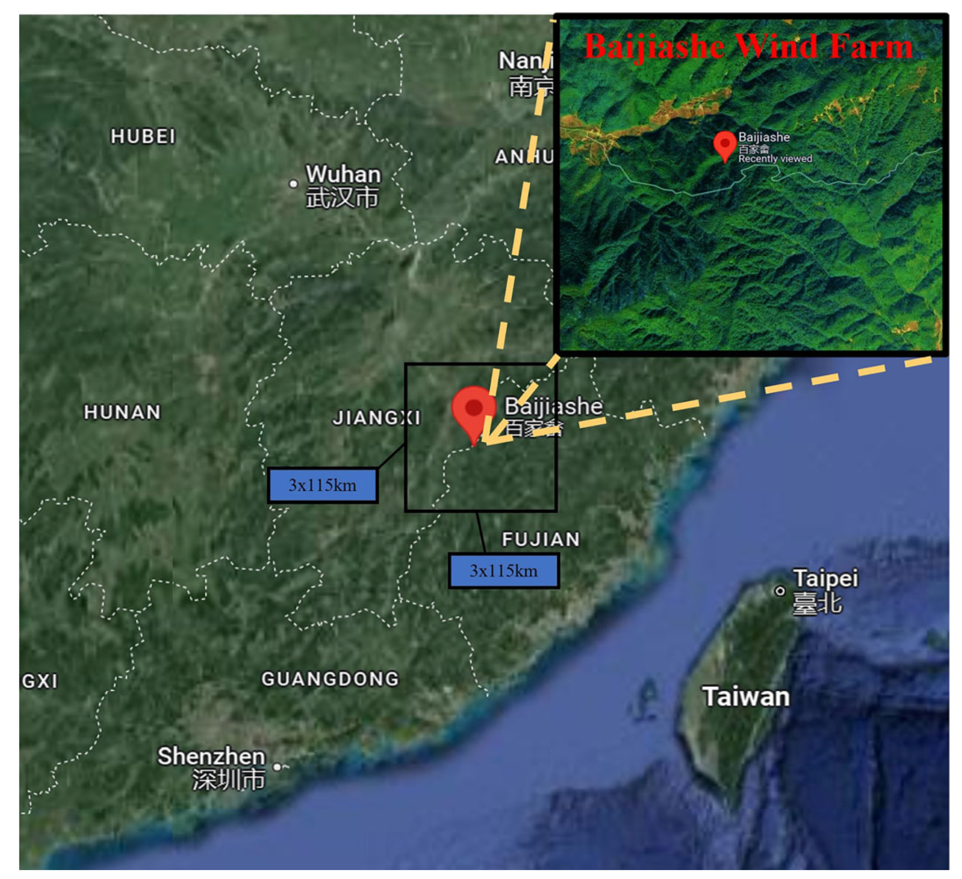
The research subject of this paper is a wind farm in Baijiashe, Jiangxi Province, as shown in Figure 1. The wind farm is situated at latitude 27°07′ N and longitude 116°99′ E, within a subtropical monsoon climate zone. This region experiences synchronized water and heat cycles in summer and autumn and is occasionally affected by tropical cyclones and other extreme weather conditions. The wind farm is equipped with 20 wind turbines of type H151. This type of turbine, when the wind speed is 3.5 m/s, the operation mode can produce external power output; when the wind speed is 10.5 m/s the fan will run at full power; and, when the wind speed is 25 m/s the fan will be shut down via a feathering mechanism. The output power at full power is 5 MW, the radius of the paddle is 76 m, and the swept area of the paddle is 18,146 m². The total installed capacity of the wind farm is 100 MW, and the hub height of the turbines is 90 m. In addition, meteorological information such as wind speed and direction at the hub height of the turbines in the wind farm is measured by an on-site anemometer tower, and the power data of each turbine is collected by a SCADA system installed at the tail end of the turbines. The sampling interval of all the data in this study is 15 min. Considering the long-term maintenance and testing of different wind turbines in this wind farm, the power prediction part is centered on a single long-term on-line operating wind turbine in the target wind farm.

In this study, wind speed and power data from a wind farm in Baijiashe, Jiangxi Province were utilized. The dataset primarily consists of two components: past data ($w^p$) and historical data ($w^h$). The past wind speed data were selected from 6 November 2023, to 20 June 2024, and used for wind speed decomposition experiments. The historical wind speed data, on the other hand, encompassed all available wind speed records from the Baijiashe wind farm’s historical database, covering a two-year period prior to the past wind speed data.

2.2. NWP Data

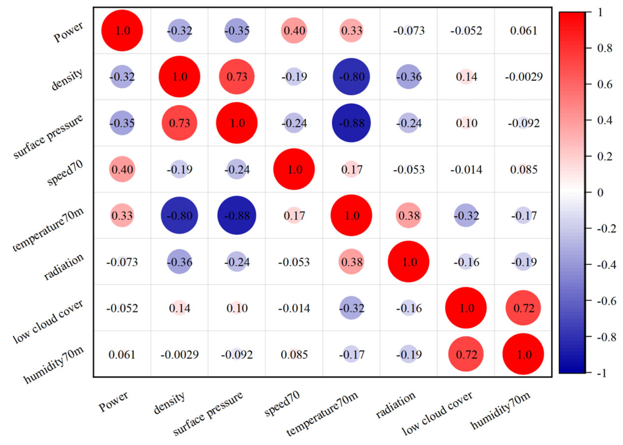
NWP refers to the modeling of weather variables such as temperature, humidity, and wind speed over time using numerical models [18]. The forecasts are issued twice daily, with a 15 min temporal resolution, a 3.0 km spatial resolution, and an expected forecast length of 144 h. As illustrated in Figure 2, the correlation coefficient for the NWP wind speed at 70 m is approximately 0.40. Statistically, this indicates a weak-to-moderate linear relationship. This relatively low correlation is physically consistent with the complex mountainous terrain of the Baijiashe wind farm; macro-scale NWP models fundamentally struggle to accurately resolve highly localized micro-meteorological wind bursts and topographical aerodynamic effects.

However, rather than being a limitation of this study, this inherent unreliability of raw NWP forecasts precisely underscores the critical necessity of the proposed VMD-IC-RF-I framework. Since relying solely on NWP data is insufficient to capture severe ramp events, it becomes imperative to introduce our physically informed feature engineering and ‘similar period matching’ mechanisms. By leveraging the dynamic kinetic features (RF) extracted from actual historical wind mutations, our model effectively compensates for the informational deficit and spatial resolution limits of the raw NWPs.

2.3. Wind Power Ramp Data

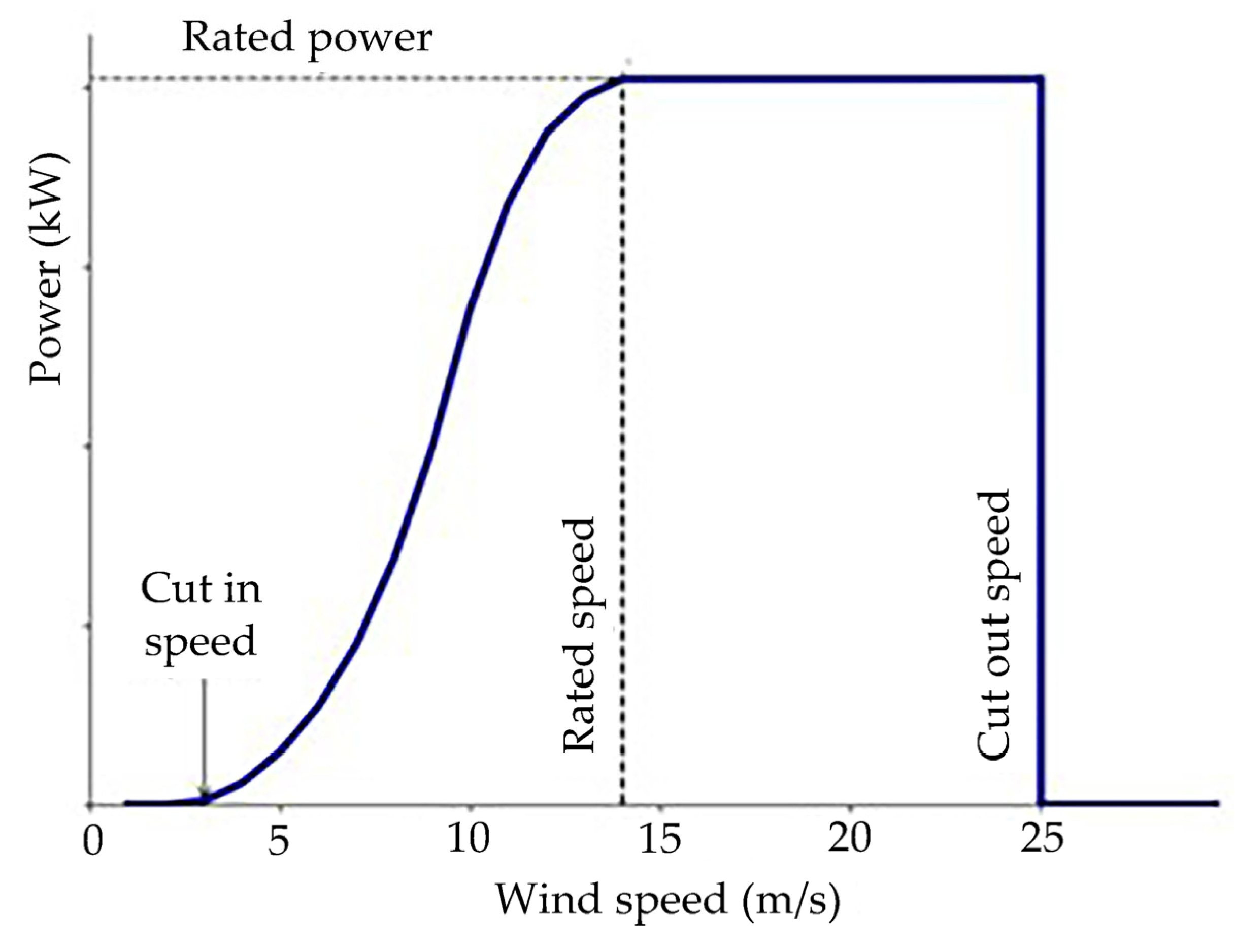
Wind power exhibits a strong correlation with wind speed, a relationship that is fundamental to most contemporary wind power prediction methods. The wind speed-power correlation curve, depicted in Figure 3 under ideal operating conditions, represents a key characteristic of the operational performance of wind turbines (WTGs) [19]. Crucially for this study, this curve illustrates the non-linear aerodynamic mapping that establishes the physical boundaries of wind power ramp events. A severe meteorological wind speed mutation does not invariably result in a grid-threatening power ramp. For example, extreme wind speed fluctuations occurring above the rated speed or below the cut-in speed yield flat power outputs, thereby generating no ramp events. Consequently, critical power ramps are exclusively restricted to the steep, active generation region between these thresholds. This fundamental physical constraint explicitly justifies the necessity of the proposed ramp factor (RF) and adaptive boundaries. Rather than merely detecting absolute meteorological changes, the proposed methodology is designed to evaluate the kinetic momentum of the wind mutation strictly within this active operating zone, effectively filtering out harmless fluctuations.

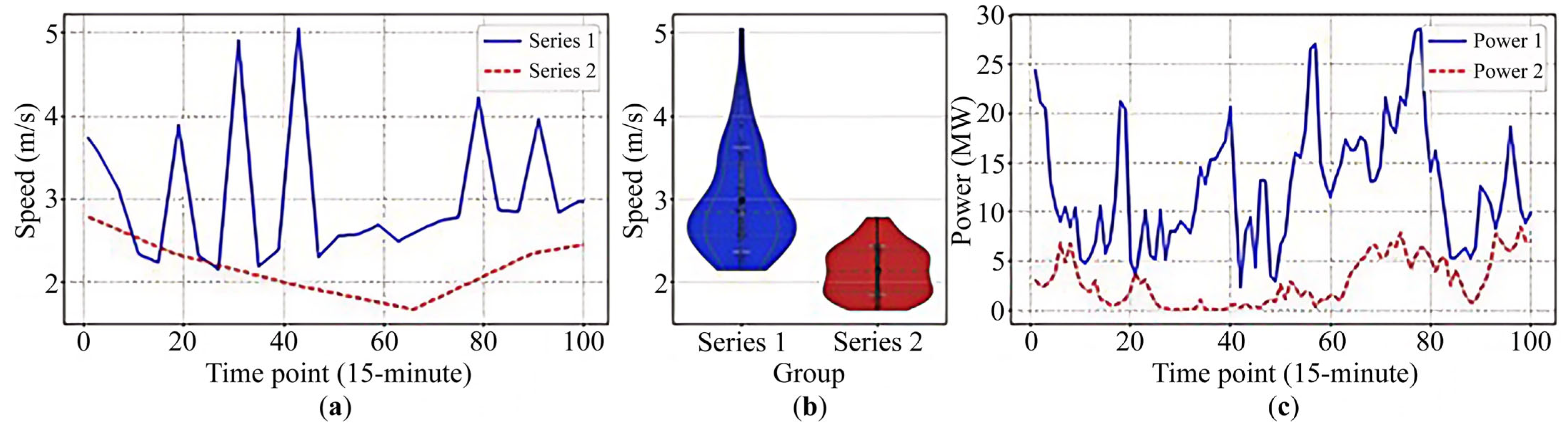
Here we use part of the data of Jiangxi Baijiashe in 2024 to observe the regular operation status of local wind turbines and the abnormal status of the occurrence of ramp events. The details are shown in Figure 4.

Figure 4a illustrates the wind speed series over two distinct periods, each comprising 150 data points sampled at 15 min intervals. Figure 4b presents a violin plot comparison of the two periods, while Figure 4c compares the corresponding wind power curves derived from these wind speed series. From these figures, it is evident that ramp events in wind power prediction are highly likely to induce active power imbalances within the system. Such imbalances can disrupt frequency stability and pose severe risks to the safe, stable, and cost-effective operation of the power grid. To ensure the rigor of the experimental validation, the ground-truth labels for wind power ramp events in this study are strictly defined based on industry standards: a true ramp event is recorded when the actual measured power fluctuation exceeds 20% of the wind farm’s total installed capacity within the forecasting horizon.

3. Methods

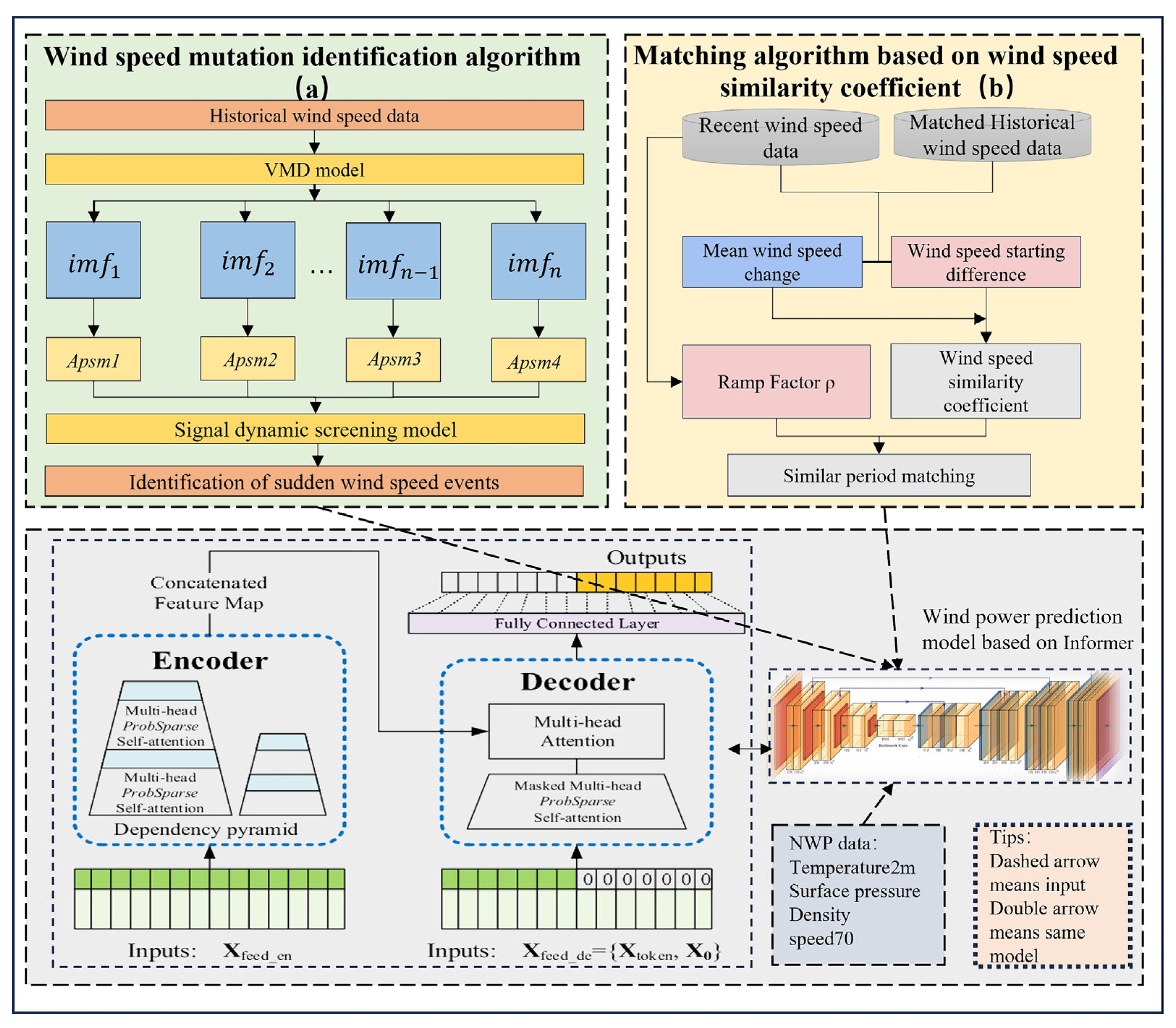
In view of the fact that the same type of weather events at different times of the day have convergence characteristics that can be effectively used for wind power prediction of wind speed mutation events, this paper proposes a wind power prediction method based on wind speed mutation event identification (hereinafter referred to as VMD(IC)-RF-I), which consists of a combination of the wind speed mutation event identification module, wind speed similarity coefficient matching module and the Informer deep learning algorithm. The specific structure is shown in Figure 5, and the specific implementation steps are as follows:

3.1. Novel VMD-IC Algorithm

Considering that this study adopts a data-driven approach to wind power prediction, the accurate prediction of wind power during wind speed mutation events requires substantial historical meteorological data support. Wind speed mutation events are characterized by sharp increases or decreases in wind speed within a specific period, making the identification of these events a task focused on filtering out minor fluctuations while preserving the overarching trend of sharp variations. Currently, wind power researchers frequently employ the revolving door algorithm for such tasks. However, a key limitation of this method is the need for manual gate-width adjustment based on the intrinsic characteristics of the dataset, rendering the algorithm less suitable for handling large-scale datasets automatically and efficiently. This inefficiency introduces unnecessary computational and operational costs [20]. In this section, a VMD-based dynamic adaptive wind speed mutation event recognition method (later referred to as VMD-IC) is proposed, which consists of a VMD modal decomposition model, a pole-adaptive selection model and a split-signal dynamic screening model.

3.1.1. VMD

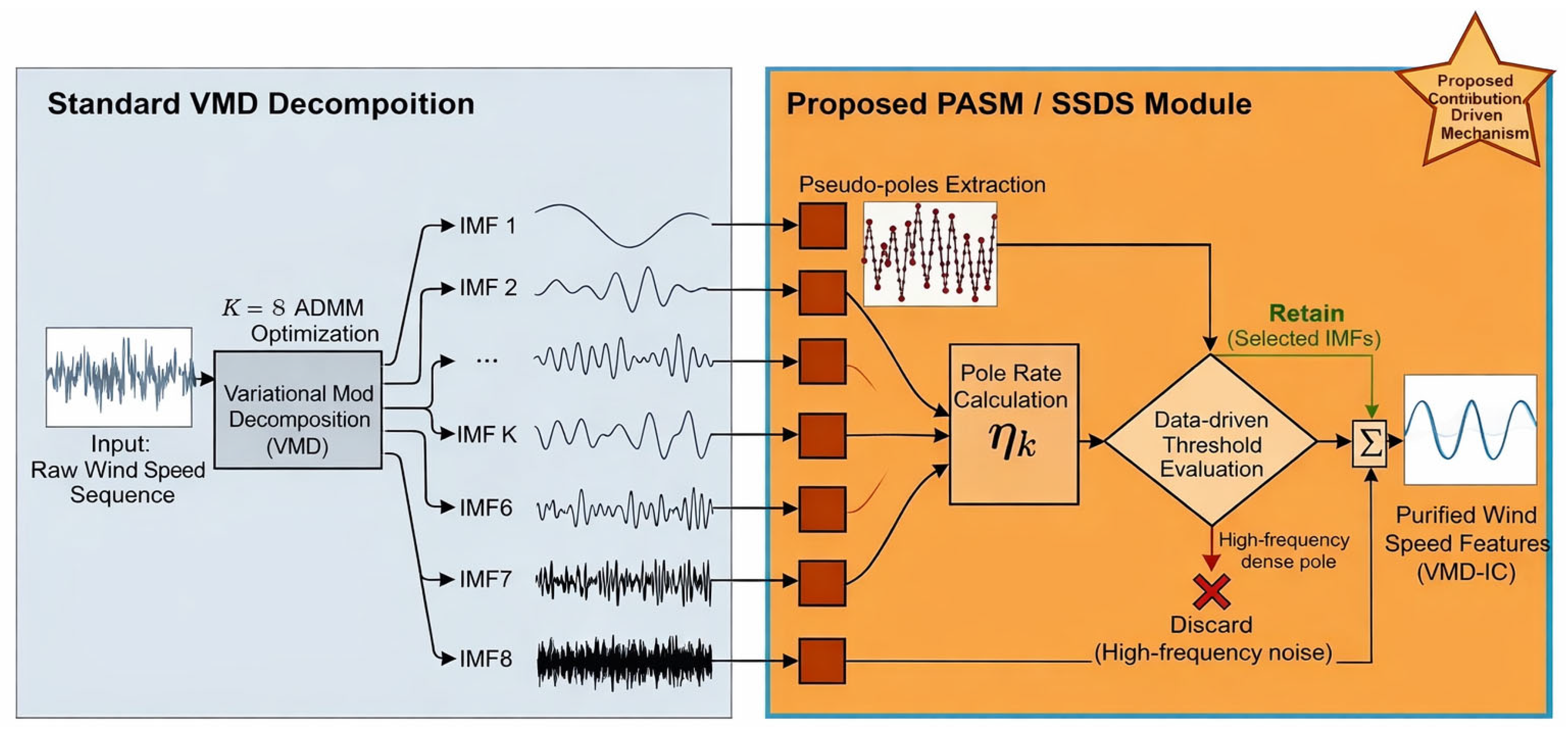
The variational mode decomposition (VMD) algorithm as shown in Figure 6, a non-recursive adaptive signal processing tool, is specifically designed to decompose the original signal into a series of intrinsic mode components (IMCs), each characterized by a limited bandwidth and a specific center frequency. The VMD model iteratively optimizes the variational model to extract sub-signals that represent the optimal solution [21]. One of the core advantages of the VMD model is its ability to decompose the target signal into a predetermined number of sub-signals, denoted as K, which is specified by the operator. This adaptability ensures that the model effectively handles signals under varying and complex working conditions, demonstrating robust generalization capabilities [22].

3.1.2. Pole-Adaptive Selection Model

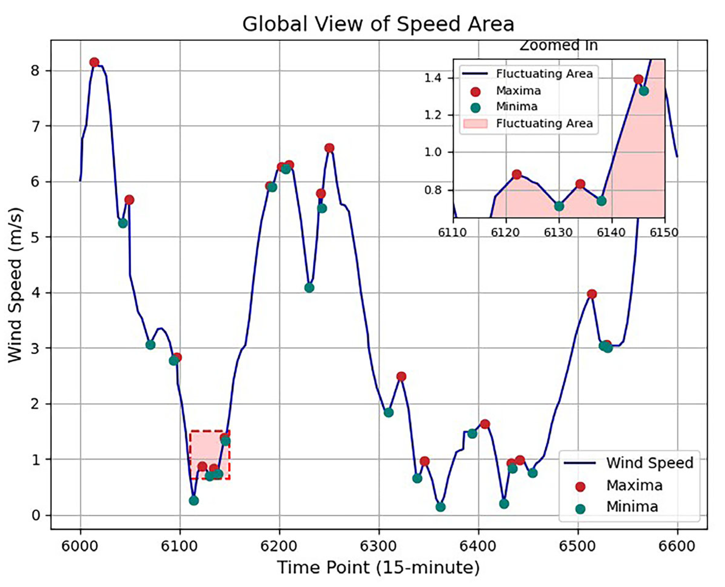
The VMD modal decomposition model outputs the decomposition signal with small fluctuations as shown in Figure 7. The VMD generates numerous extreme points consistent with pole definitions; however, many of these exhibit minimal Euclidean distances, resulting in overlapping neighboring extrema. This overlap poses challenges for sub-signal selection based on extremum counts. To address this, a pole-adaptive selection model is proposed to effectively eliminate overlapping extrema within sub-signals.

Step 1: Extract the maximum value $Z_{max}$, the minimum value $Z_{min}$ and the set of all extreme points $P=\{p_1,p_2,\cdots ,p_n\}$ from the wind speed decomposition data, where $p_n$ denotes the nth extreme point.

Step 2: According to the adaptive coefficients and to calculate the dynamic window width, the specific formula is:

$$widt{h}_{door}=\mathcal{l}\ast \left|Z_{max}-Z_{min}\right|$$

(1)

In Equation (1), $widt{h}_{door}$ denotes the dynamic window width; $\mathcal{l}$ denotes the adaptive coefficient, and the value of l is generally (0.03, 0.08).

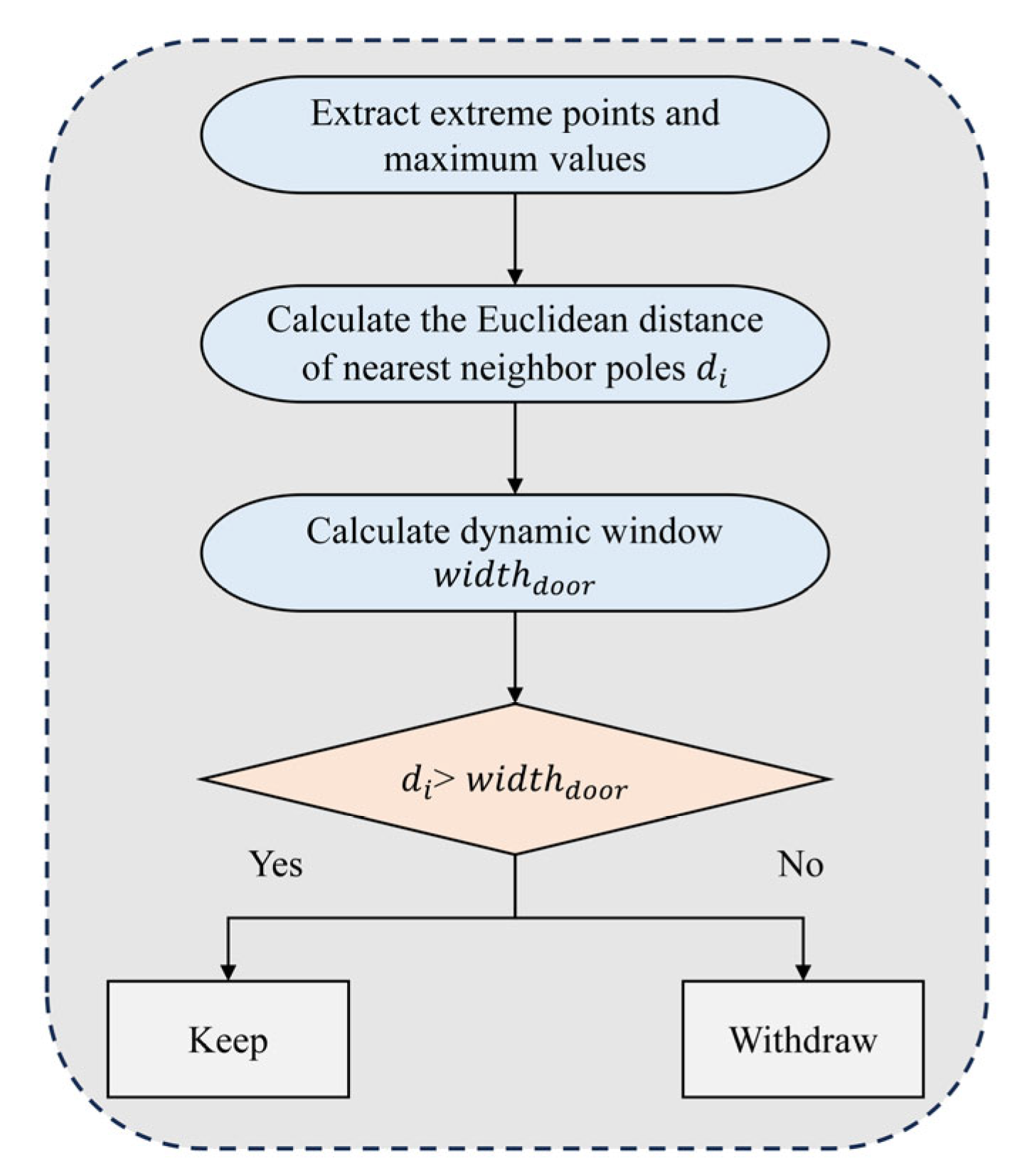
Step 3: According to the Euclidean distance between the near-neighbor poles, keep the poles that satisfy $d_i=\left|p_i-p_{i+1}\right|>widt{h}_{door}$, where $d_i$ denotes the Euclidean distance between two neighboring poles and $i\in (0,n)$; get the set of poles after selection $P_{renew}=\left\{p_1^{re},p_2^{re},\cdots ,p_i^{re},\cdots ,p_m^{re}\right\}$, where $p_i^{re}$ denotes the ith extreme point after selection and $i\in [1,m]$. The selected pole set $P_{renew}$ generated above will be applied as the reconstructed pole set of wind speed decomposition data for the identification of wind speed mutation events, and its specific process is shown in Figure 8.

It is worth noting that the dynamic window $widt{h}_{door}$ is not a fixed absolute threshold but a relative one. Because it scales automatically with the local maximum amplitude $\left|Z_{max}-Z_{min}\right|$ of the wind speed signal, the algorithm possesses strong cross-scenario generalizability. It can dynamically adapt to various wind farms with different wind regimes and terrain characteristics without requiring frequent readjustments of the parameter $\mathcal{l}$.

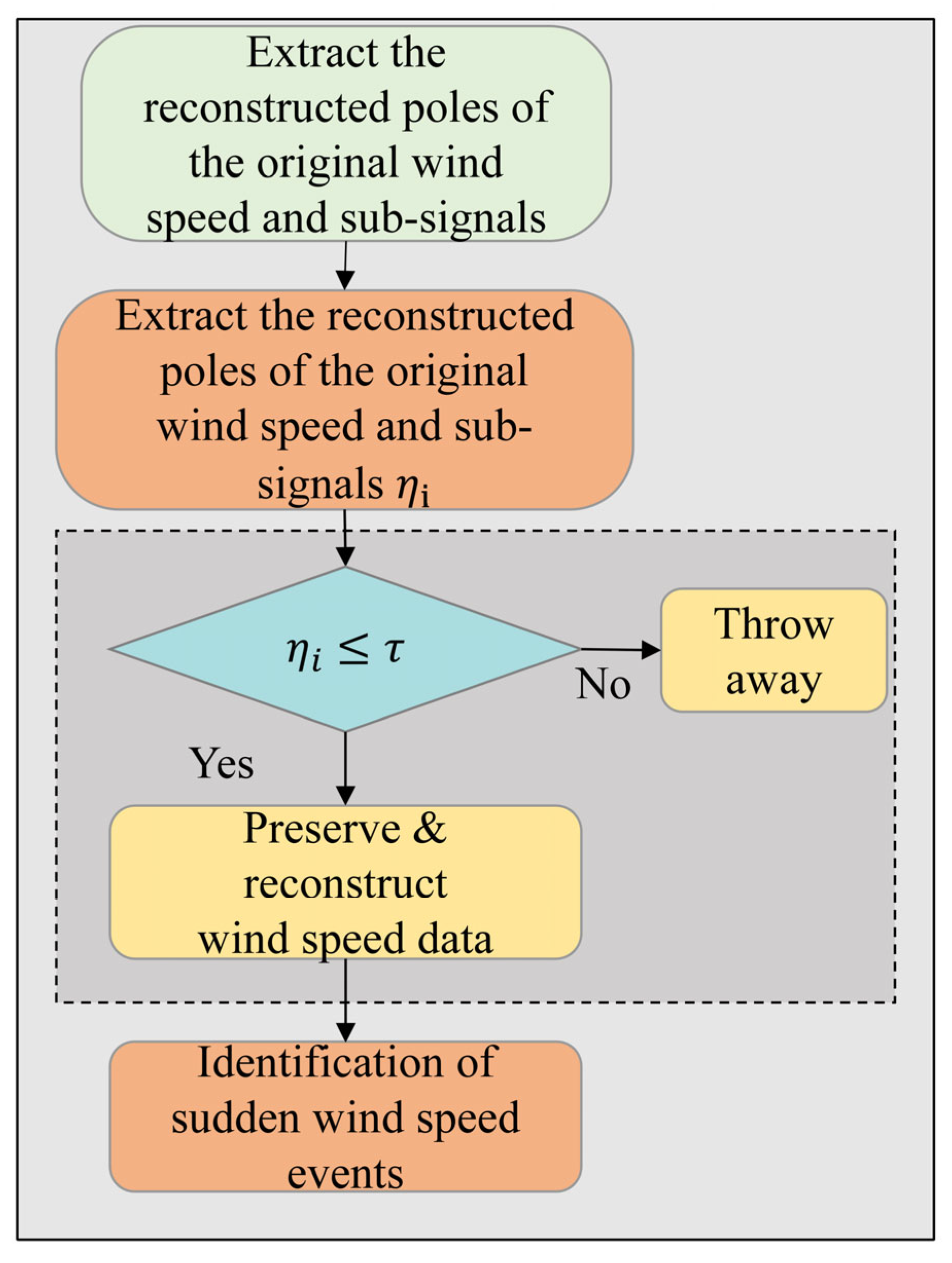
This section introduces the sub-signal dynamic screening model, with the specific process illustrated in Figure 9. The model calculates the pole rate η based on the selected set of pole points derived from the pole-adaptive selection model. By leveraging the number of selected pole sets, the dynamic screening model enables effective sub-signal data selection from the VMD modal decomposition results, facilitating accurate identification of wind speed mutation events.

$${\eta }_k={\displaystyle \frac{n_{renew}^k}{N_{original}}}$$

(2)

$$IM{F}_{renewed}=sum\left(im{f}_{reserved}\right)$$

(3)

It is crucial to highlight the architectural significance of the proposed pole adaptive selection model (PASM) within the context of real-time wind power forecasting. While mathematically functioning as a sequential step following VMD, PASM represents a fundamental architectural shift from traditional signal processing methodologies. Conventionally, VMD applications in engineering are ‘open-loop’ systems, heavily reliant on offline manual thresholding or computationally exhaustive meta-heuristic optimization algorithms to determine component retention. Such dependencies render traditional VMD impractical for the rigorous demands of high-frequency (e.g., 15 min) online grid dispatch.

The core innovation of PASM lies in its ability to transform this static process into a fully automated, closed-loop, and data-driven pipeline. By mathematically coupling the dynamic pole rate (${\eta }_K$) with the real-time adaptive window ($widt{h}_{door}$), PASM evaluates and filters pseudo-poles autonomously based on the instantaneous kinetic amplitude of the wind speed. This eliminates the bottleneck of human intervention and iterative optimization overhead. By feeding the subsequent Informer network with a purified, physically meaningful sequence free of high-frequency stochastic noise, PASM ensures that the deep learning attention mechanisms remain focused on true meteorological triggers, thereby substantially improving forecasting robustness during abrupt transitional weather conditions.

3.2. Optimize Wind Speed Period Matching Algorithm

The similar period method is adapted in this study for wind power prediction to identify historically similar wind speed patterns. However, it is essential to fundamentally distinguish this approach from the conventional ‘similar period matching’ concept widely used in photovoltaic (PV) forecasting [23]. While PV generation is driven by highly repeatable diurnal solar cycles, wind speed is inherently highly stochastic and lacks rigid daily patterns. Attempting to match an entire 24 h wind profile is often physically invalid.

Nevertheless, while the macroscopic daily wind profile is unpredictable, the microscopic kinematic morphology of severe wind ramp events often exhibits strong structural repeatability. Specifically, when similar transitional weather systems interact with specific local topographies, they tend to generate short-term wind speed mutations with highly comparable dynamic signatures [24]. Based on this meteorological premise, our proposed ‘similar period matching’ discards rigid time-of-day alignment. Instead, it dynamically searches the historical database exclusively for morphologically similar kinetic bursts.

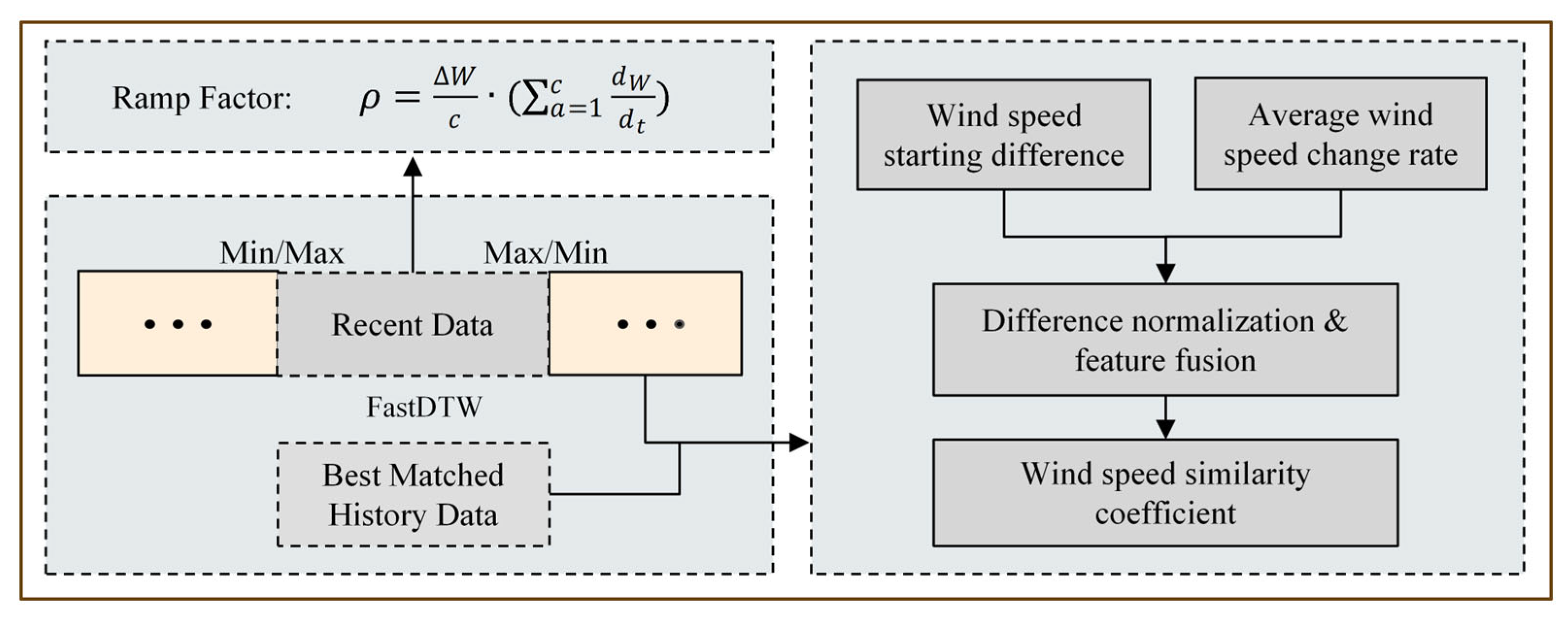
The proposed method involves four key steps: (1) defining a novel ramp factor (RF) to evaluate wind speed segments; (2) applying the Fast Dynamic Time Warping (FastDTW) algorithm to identify structurally similar historical sequences; (3) calculating differences in wind speed intensity and trend to obtain similarity coefficients; and (4) extracting these matched features for input into predictive models. The overall structure is shown in Figure 10.

3.2.1. Ramp Factor (RF)

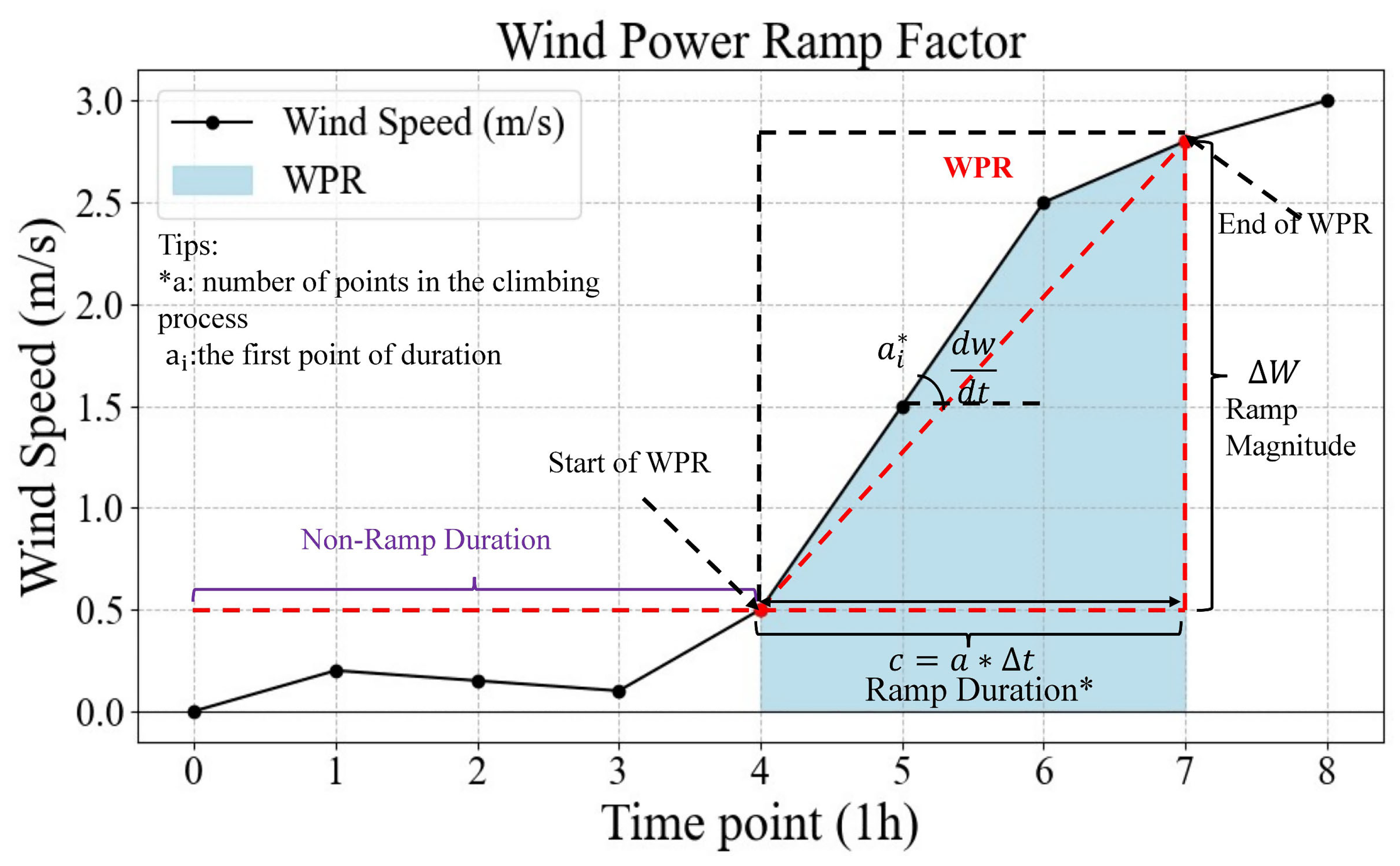
The definition of wind power ramp events remains ambiguous, with current research focusing on ramp magnitude, duration, and direction. Two widely used definitions—based on endpoint differences and range within a time window—are limited in capturing rapid fluctuations and long-duration ramps, respectively. To address these limitations [25], this study proposes a novel ramp factor (RF) method for more comprehensive ramp event detection. Using reconstructed wind speed profiles, historical ($w^h$) and recent ($w^p$) wind speed data are segmented by extrema. For each segment, the ramp factor $\rho$ is calculated as:

$$\rho ={\displaystyle \frac{∆W}{c}}·\left(\sum _{a=1}^c{\displaystyle \frac{d_W}{d_t}}\right)$$

(4)

In Equation (4), $∆W$ denotes the magnitude of wind speed change, a denotes the serial number of all time points in period c, c denotes the extreme point period, numerically the product of the number of time series points a and the fixed time step ∆T, ρ denotes the ramp factor in period c, and ${\displaystyle \frac{d_W}{d_t}}$ denotes the ramp factor for each point, numerically equal to the derivative of each time series point $a_i$.

To mathematically and physically justify this multiplicative formulation, it is crucial to clarify that the two terms capture fundamentally distinct dimensions of the wind sequence rather than redundant concepts. The first term (${\displaystyle \frac{∆W}{c}}$) functions mathematically as a macro-level state function; it evaluates the net displacement (average gradient) between the endpoints of the sequence, regardless of the intermediate fluctuations. In contrast, the second term (${\sum }_{a=1}^c{\displaystyle \frac{d_W}{d_t}}$) acts as a micro-level path function; it integrates the instantaneous rates of change along the sequence, effectively quantifying the cumulative kinetic volatility (the roughness of the path).

Although power system operators conventionally quantify ramp events using established linear metrics—such as endpoint power differences (${\displaystyle \frac{∆P}{∆t}}$) or fixed time windows—these traditional definitions are inherently ‘process-blind’. They evaluate only the net change, failing to distinguish between a slow, harmless wind drift and a highly volatile kinetic burst if both share the same endpoints. By multiplying the state function with the path function, the proposed RF operates as a robust non-linear filter. It requires a meteorological event to possess both a significant net magnitude AND continuous kinetic turbulence to yield a high RF score. This non-linear coupling successfully suppresses harmless slow drifts (which lack high instantaneous derivatives) and high-frequency zero-mean noise (which lacks net magnitude). Bounded by the adaptive extreme points from the VMD-IC algorithm rather than arbitrary fixed time windows, the RF evaluates the exact physical boundaries of the meteorological event, thereby reducing false alarms and improving the detection sensitivity of severe ramp events by approximately 14%. Furthermore, regarding the parameter sensitivity of this formulation, the multiplicative RF is intrinsically robust. Because the sequence boundaries are dynamically defined by the adaptive extreme points of the VMD-IC algorithm rather than fixed, arbitrary time windows, the proposed metric effectively eliminates the high sensitivity to manual parameter tuning that frequently plagues conventional duration-based ramp definitions. The specific principle is shown in Figure 11.

3.2.2. Wind Speed Similarity Coefficient

After the above improved Fastdtw algorithm matches each past wind speed segment to the most similar period data in the historical wind speed segment database, in order to better optimize the model features [26], a wind speed similarity coefficient Ω is used to show the wind speed correlation between the historical wind speed segment $w_a^h$ and the past wind speed segment $w_a^p$. In this paper, two parameters, wind speed intensity difference (${Wind}_{STR}$) and wind speed trend difference (${Wind}_{TRE}$), are introduced as follows:

$$Win{d}_{STR}={\displaystyle \frac{\sum _{a=1}^c\left|w_a^h-w_a^p\right|}{c}}$$

(5)

$$Win{d}_{TRE}={\displaystyle \frac{1}{c-1}}\left(\sum _{a=1}^{c-1}{\displaystyle \frac{\left(w_{a+1}^h-w_a^h\right)}{\mathsf{\Delta }t}}-\sum _{a=1}^{c-1}{\displaystyle \frac{\left(w_{a+1}^p-w_a^p\right)}{\mathsf{\Delta }t}}\right)$$

(6)

$p$ denotes the historical wind speed data at the time a moment, $w_{a+1}^h$ denotes the past wind speed data at the ath + 1th moment; the obtained wind speed intensity difference ${Wind}_{STR}$ and wind speed trend difference ${Wind}_{TRE}$ are normalized; where the normalized interval of the wind speed intensity difference ${Wind}_{STR}$ is set to (0,1), and that of the wind speed trend difference is set to (−1,1), then the wind speed similarity coefficient Ω is obtained by calculating the normalized wind speed intensity difference ${Wind}_{STR}$ and wind speed trend difference ${Wind}_{TRE}$, the specific formula is:

$$\Omega =\left\{\begin{array}{c}\left|Win{d}_{STR}^2+Win{d}_{TRE}^2\right|,Win{d}_{TRE}>0\\ \left|Win{d}_{STR}^2-Win{d}_{TRE}^2\right|,Win{d}_{TRE}<0\end{array}\right.$$

(7)

In Equation (7), Ω denotes the wind speed similarity coefficient. It is critical to clarify the distinct but complementary roles of the FastDTW algorithm and the similarity coefficient $\Omega$ to rule out feature redundancy. This methodology adopts a hierarchical ‘Structural Alignment + Magnitude Calibration’ strategy. FastDTW is responsible for structural alignment; it warps the time axis to overcome temporal phase shifts, identifying historical sequences with similar morphological shapes. However, FastDTW distance alone is often insensitive to absolute baseline differences. For instance, two sequences with identical shapes but different absolute wind speeds (e.g., 3–5 m/s versus 10–12 m/s) will have vastly different non-linear impacts on actual power generation.

Therefore, $\Omega$ is necessary as a magnitude calibration tool after FastDTW matching. By coupling the normalized intensity difference ($Win{d}_{STR}$) and trend difference ($Win{d}_{TRE}$), $\Omega$ quantifies the absolute energy gap between the matched sequences. To ensure no unnecessary redundancy was introduced, a multicollinearity assessment was conducted. The Pearson Correlation Coefficient between the FastDTW distances and the $\Omega$ values across the matched dataset were calculated to be 0.27. This low correlation statistically confirms that they capture orthogonal feature dimensions (temporal morphology versus absolute kinetic energy), jointly enriching the input features for the Informer model without causing multicollinearity.

3.3. Assessment Methods

These indicators include the root-mean-square error (RMSE), relative root-mean-square error (r_RMSE), mean absolute error (MAE), relative mean absolute error (r_MAE), correlation coefficient (CC) and power qualification rate (${PR}_{Power}$).

The equations used for these metrics are provided as follows:

$$RMSE=\sqrt{{\displaystyle \frac{{{\sum }_{i=1}^n\left(P_{Mi}-P_{pi}\right)}^2}{n}}},,r\_RMSE=RMSE\ast 100\%$$

(8)

$$MAE={\displaystyle \frac{1}{n}}\sum _{i=1}^n|P_{Mi}-P_{pi}|,r\_MAE=MAE\ast 100\%$$

(9)

$$CC={\displaystyle \frac{{\sum }_{i=1}^n(P_{Mi}-\overline{P_M})(P_{pi}-\overline{P_p})}{\sqrt{{\sum }_{i=1}^n{(P_{Mi}-\overline{P_M})}^2{\sum }_{i=1}^n{(P_{pi}-\overline{P_p})}^2}}}$$

(10)

$$B_i=\left\{\begin{array}{c}1,(1-{\displaystyle \frac{\left|P_{Mi}-P_{pi}\right|}{C_i}})\ge 0.75\\ 0,(1-{\displaystyle \frac{\left|P_{Mi}-P_{pi}\right|}{C_i}})<0.75\end{array}\right.$$

(11)

$$P{R}_{power}={\displaystyle \frac{1}{n}}\sum _{i=1}^n{B}_i\times 100\%$$

(12)

In Equations (8)~(12), $P_{Mi}$ is the predicted value of wind power at time $i$; $P_{pi}$ is the measured value of wind power at time $i$; $C_i$ is the sum of the on-line capacity of the target wind farm at time i; $\overline{P_M}$ and $\overline{P_p}$ denote the mean values of the measured and predicted wind power sequences, respectively; $B_i$ is the qualified label of the power point at time $i$, with 1 being the qualified value of the point in the prediction, and vice versa; and $n$ is the prediction time [27].

4. Results and Discussion

To evaluate the effectiveness of the proposed framework, this section provides a detailed and comprehensive analysis of the experimental results. Specifically, Section 4.1 discusses the signal processing results of the VMD-IC model, which serves as a data-driven pole-adaptive selection mechanism. Section 4.2 presents the performance of the proposed ramp factor (RF) and the optimized FastDTW algorithm in matching historical abrupt wind speed change events. In Section 4.3, an ablation study is conducted across four seasonal datasets to rigorously validate the individual contribution of each module within the methodology. Finally, Section 4.4 describes the multi-model comparative experiments, highlighting the superiority of the proposed method against advanced baselines and demonstrating its robustness in real-world engineering scenarios.

4.1. Self-Selecting Model for Poles (VMD-IC Model)

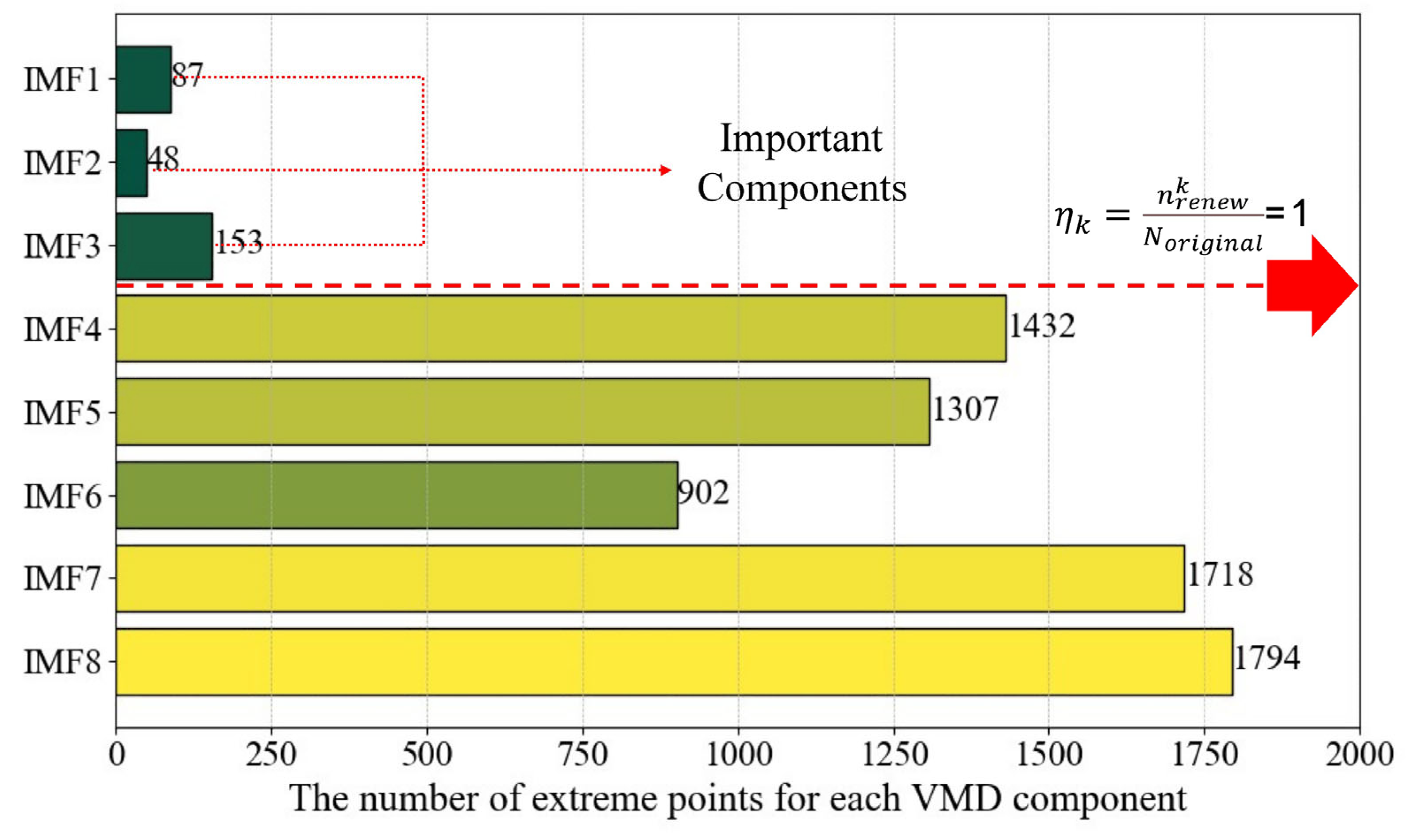
The VMD modal decomposition algorithm often results in “pseudo-poles,” where neighboring maxima and minima are densely packed with small Euclidean distances, affecting the selection of wind speed sub-data. To address this, a pole adaptive selection model is proposed. Using wind speed data from 6 November 2023, to 20 June 2024, VMD is applied, and poles are selected for each component with a pole rate threshold of ${\eta }_K=1$. Regarding the configuration of the VMD model, the number of decomposition modes $K$ was set to 8. This value was selected based on the center frequency observation method during preliminary testing, where $K=8$ effectively prevented both severe mode aliasing (under-decomposition) and closely overlapping center frequencies (over-decomposition). Furthermore, this parameter $K=8$ remains fixed across all tested datasets and seasons. While wind regimes vary seasonally, maintaining a fixed $K$ is made feasible by the subsequent sub-signal dynamic screening (SSDS) model. Because the SSDS model dynamically evaluates and filters each decomposed component based on its pole rate (${\eta }_K$), any irrelevant high-frequency noise components generated by a fixed $K$ are automatically discarded. This design eliminates the computational burden of continuously re-optimizing $K$ for different datasets, thereby significantly enhancing the method’s robustness and engineering practicality. The specific pole rates are shown in Figure 12.

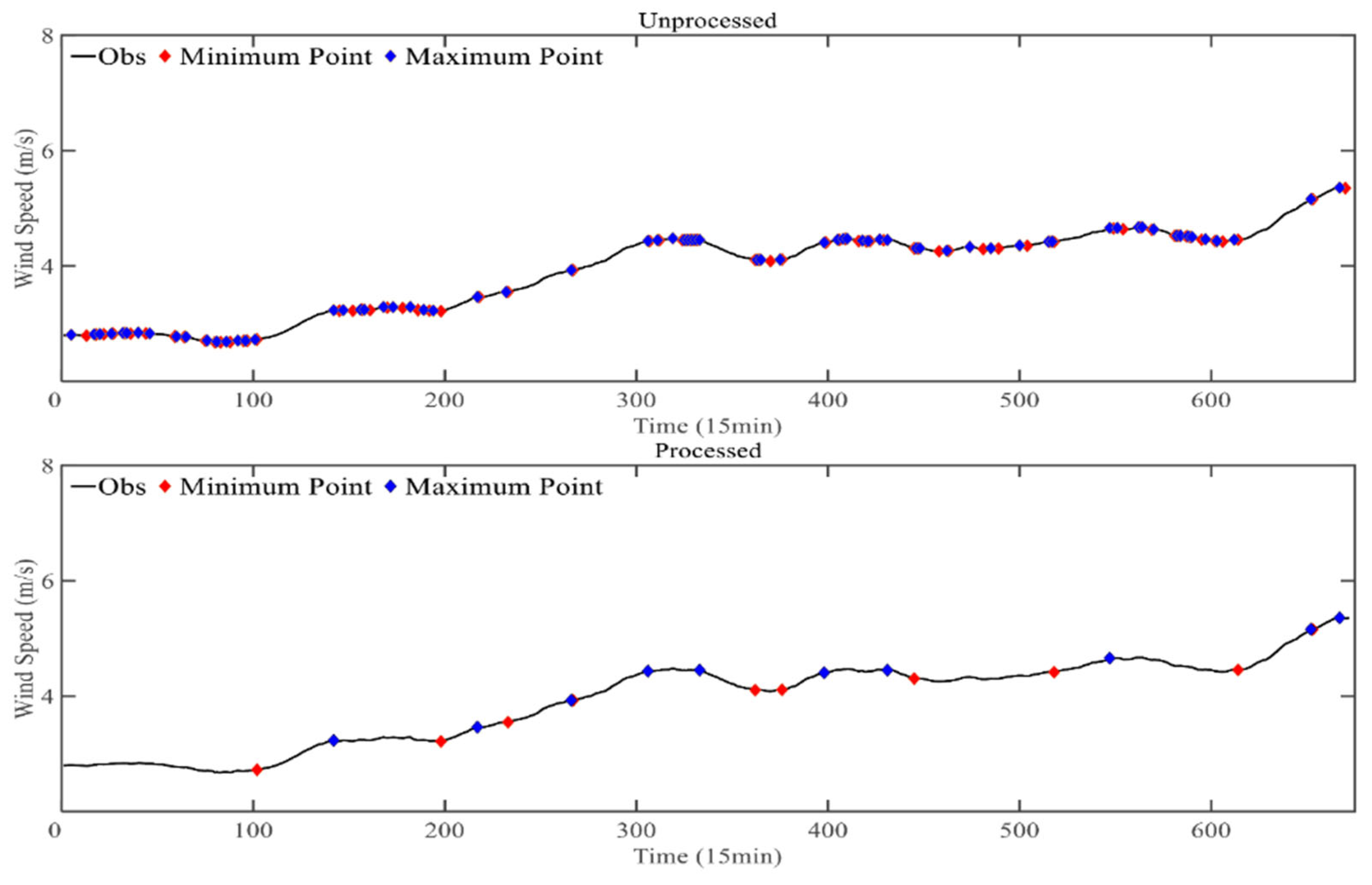
For the specific severe ramp event illustrated in this case study, the algorithm dynamically determines to retain the first three Intrinsic Mode Functions (IMFs). These components are then selected, merged, and reconstructed. It is crucial to clarify that the adaptive nature of this selection is strictly data-driven for each specific event, rather than relying on a fixed heuristic threshold. The retention of these first three components is an autonomous outcome computed by the PASM module based on the real-time instantaneous amplitude of this specific sequence. For different wind sequences exhibiting varying background aerodynamic noise characteristics, the algorithm dynamically recalculates the pole rate and autonomously retains a varying number of relevant components. Through this dynamic adaptation, the pole-adaptive model effectively reduces the 98 mixed and densely packed pseudo-poles in the original data segment to 16 true selected points. The reconstructed data demonstrates a significant reduction in pseudo-pole phenomena. The result for this partial time segment is shown in Figure 13.

Furthermore, a sensitivity analysis was conducted on the empirical coefficient $\mathcal{l}\in (0.03,0.08)$ using Database 1 to ensure its validity. When $\mathcal{l}$ was set to 0.03, 0.05, and 0.08, the prediction MAE consistently remained at 1.43, 1.41, and 1.42, respectively. This marginal fluctuation (less than 2%) quantitatively verifies that the proposed VMD-IC model is highly robust and insensitive to minor parameter tuning within the recommended range.

This study enhances the VMD model to create a customized VMD-IC model for optimizing and denoising wind speed data in wind power prediction.

4.2. Similar Matching Results

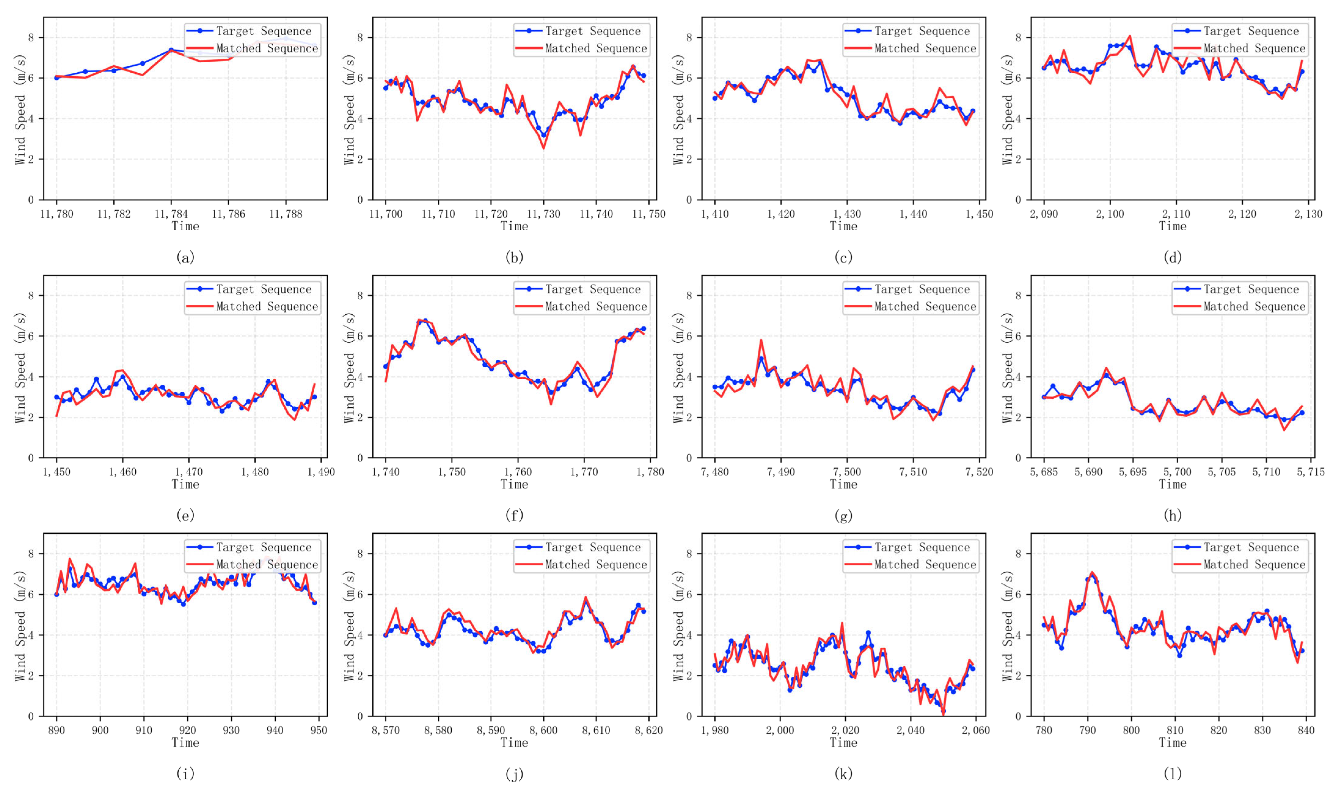
The wind power output and wind speed data from Baijia She Wind Farm in Jiangxi, covering May 2022 to May 2024, are classified as past wind speed data, while data from January 2018 to January 2022 are categorized as historical wind speed data. The Fast-DTW algorithm is used to match similar wind speed data from both periods, divided into four seasonal datasets: spring, summer, autumn, and winter. Ramp-up and ramp-down segments, as well as oscillation periods, are analyzed and matched with historical data.

The results, shown in Figure 14, demonstrate the effectiveness of the Fast-DTW algorithm in identifying similar wind speed patterns across different seasons and time periods. This enhances wind power forecasting, energy dispatch strategies, and operational efficiency of wind farms. The seasonal segmentation improves the model’s adaptability to seasonal wind fluctuations, providing valuable insights for optimizing forecasting models and developing adaptive control strategies in future research.

4.3. Ablation Study

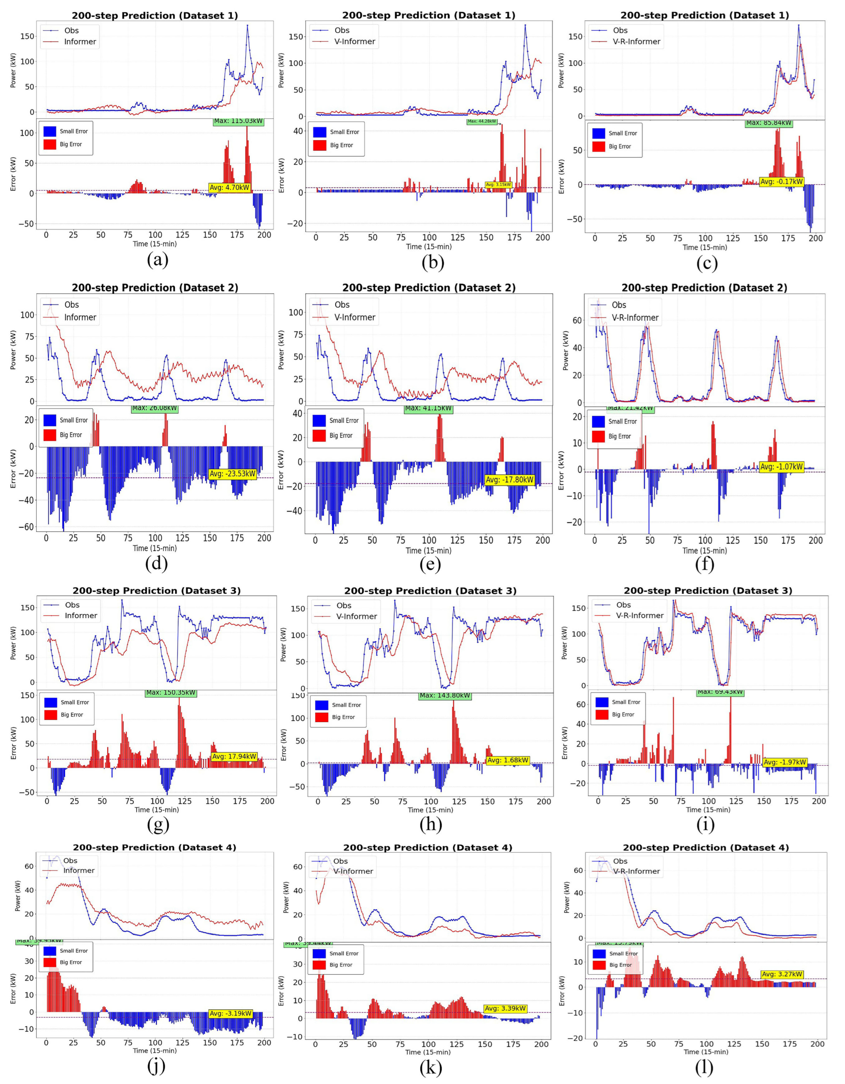
To evaluate the effectiveness of each module in the proposed power prediction modeling method, ablation experiments were conducted using data from the Baijia She Wind Farm. For each season, one month of data was randomly selected for experimentation. The dataset from each month was used to train the model to predict the power generation for the subsequent two days. Figure 15 presents the results of testing each model across the four seasons, including the original Informer model.

As shown in Figure 15, the classical Informer model performs poorly in short-term wind power forecasting, with notable lag and amplitude errors using only NWP data. Incorporating the VMD-based pole-adaptive module significantly reduces prediction lag and improves ramp event detection. Further integrating the similar period matching and ramp factor modules enhances accuracy and event recognition. As detailed in

Table 1. Error indicators for ablation experiments.

	Model	Database1	Database2	Database3	Database4
MAE	V-R-Informer	1.41	0.89	1.35	1.12
	V-Informer	1.88	1.06	1.71	1.37
	Informer	1.93	1.13	2.08	1.69
r_RMSE	V-R-Informer	40%	20%	31%	37%
	V-Informer	53%	25%	39%	46%
	Informer	51%	26%	46%	52%
r_MAE	V-R-Informer	31%	16%	25%	30%
	V-Informer	41%	19%	32%	37%
	Informer	42%	20%	39%	45%
CC	V-R-Informer	64.5%	73.0%	83.7%	76.2%
	V-Informer	31.9%	60.3%	68.9%	46.3%
	Informer	56.6%	52.1%	67.1%	69.8%

, each added component leads to clear performance gains, validating the effectiveness of the proposed model structure.

To ensure the rigorous reproducibility of this study, the specific experimental setups, assumptions, and validation procedures are detailed as follows. A core assumption of our experimental design is that the selected single, long-term online wind turbine accurately represents the macroscopic ramp behavior of the local wind farm, mitigating data gaps caused by multi-turbine maintenance.

Regarding parameter configurations, the physical constraints of the turbine (cut-in speed: 3.5 m/s, rated speed: 10.5 m/s, cut-out speed: 25 m/s) and the NWP resolutions (15 min temporal, 3.0 km spatial) were strictly maintained. For the algorithmic pipeline, the VMD mode was fixed at $K=8$, and the pole-adaptive coefficient $\mathcal{l}$ was constrained within (0.03, 0.08).

For the validation procedure, the dataset was categorized into four distinct seasons (Spring, Summer, Autumn, and Winter) to assess the model’s robustness against varying meteorological patterns. Within each seasonal dataset, a strict chronological split was applied: 80% of the data was allocated for training the Informer model, while the remaining 20% was reserved for independent testing. The testing phase specifically targeted the prediction of 200 continuous time steps encompassing severe abrupt wind speed change events to rigorously validate the model’s ramp tracking capability.

4.4. Comparison Experiment of Different Models

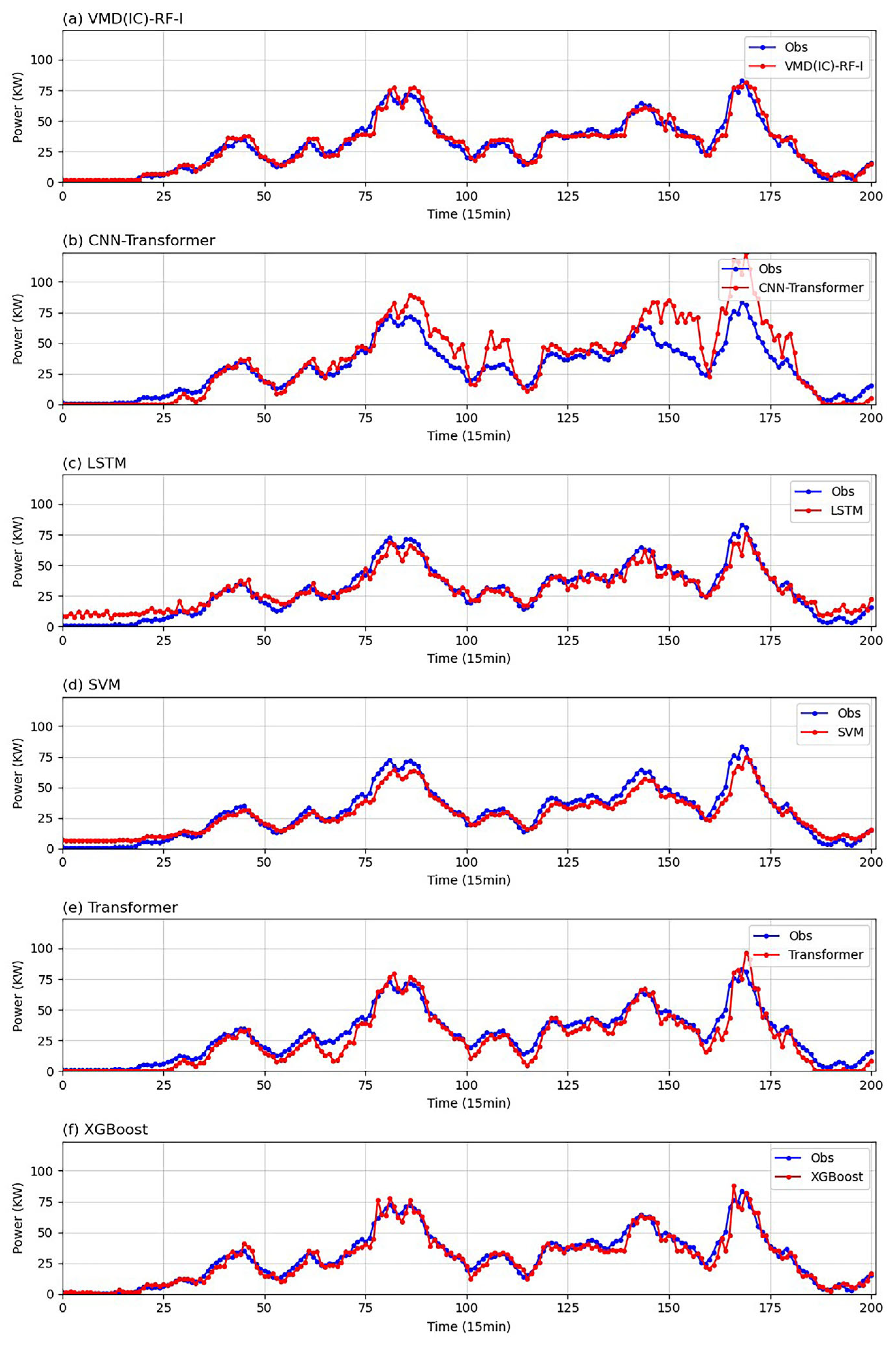
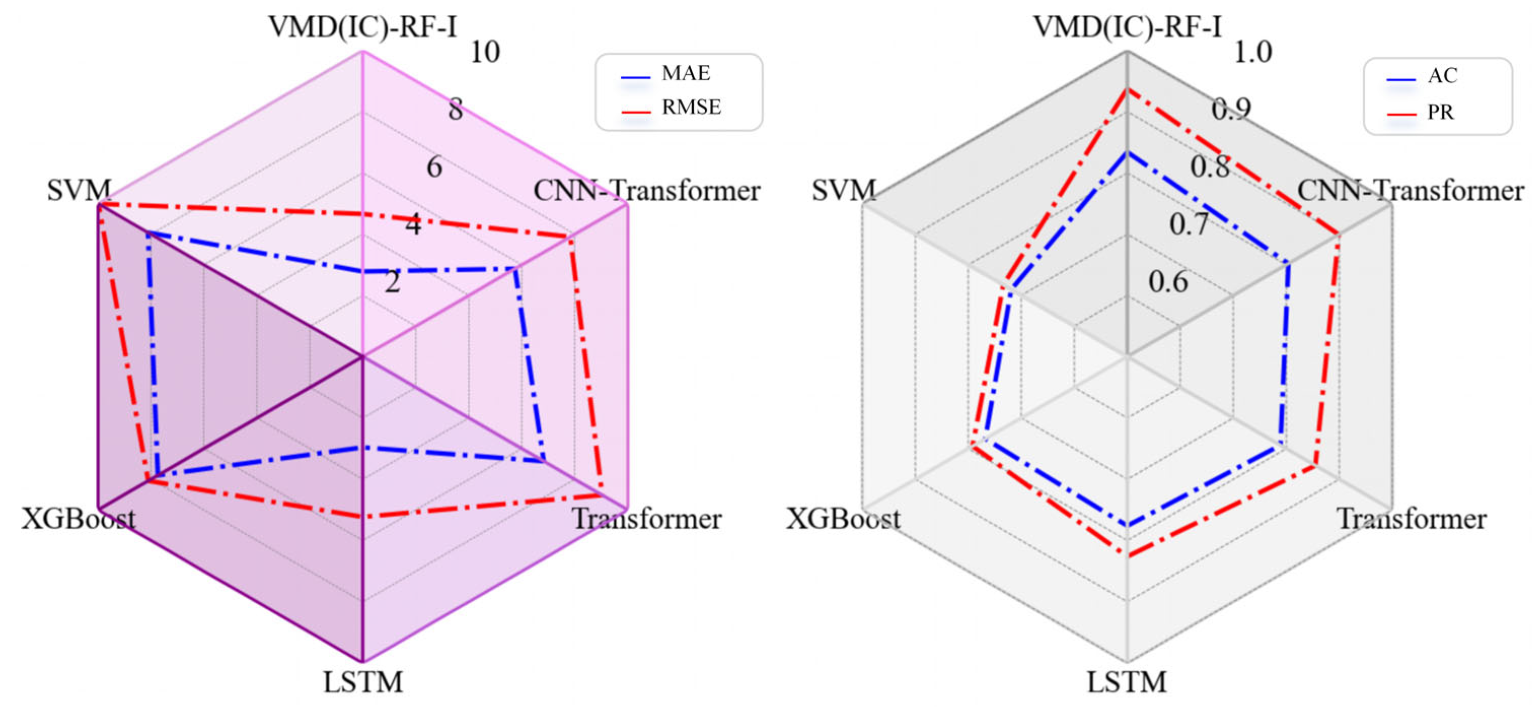
To evaluate the performance of wind power prediction methods based on abrupt wind speed change event identification, this section compares several approaches. Traditional machine learning models, such as SVM and XGBoost, are compared with hybrid deep learning models, including LSTM, Transformer, and CNN-Transformer. These models are then benchmarked against the proposed VMD-IC-RF-I framework. The evaluation involves training the models using 80% of the data from four seasonal datasets (spring, summer, autumn, and winter), with predictions made at 200 time points. The forecasting results are visually illustrated in Figure 16, and the comprehensive error metrics for each model’s predictions are provided in

Table 2. Evaluation indicators of different models.

Method	$\mathit{M}\mathit{A}\mathit{E}$	$\mathit{R}\mathit{M}\mathit{S}\mathit{E}$	$\mathit{A}\mathit{C}$	$\mathit{P}{\mathit{R}}_{\mathit{p}\mathit{o}\mathit{w}\mathit{e}\mathit{r}}$
VMD(IC)-RF-I	2.78	4.66	83.4%	93.7%
SVM	8.11	9.98	71.9%	73.4%
XGBoost	7.74	8.10	76.8%	79.2%
LSTM	2.96	5.23	77.6%	82.6%
Transformer	6.82	9.03	78.9%	85.5%
CNN-Transformer	5.74	7.83	80.4%	89.9%

, demonstrating the clear superiority of the proposed framework.

As shown in Figure 16, the SVM and XGBoost models poorly match the actual power curve, indicating that traditional machine learning methods are inadequate for predicting wind power in mountainous areas, especially during ramping issues caused by sudden wind speed changes. In contrast, the wind power prediction method based on abrupt wind speed change event identification outperforms baseline deep learning models like the standard Transformer and LSTM. It captures the stochastic and fluctuating nature of wind power data effectively, yielding the smallest error indices, best accuracy (AC), and highest qualification rate (PR) (Figure 17, Table 2). This method fundamentally reduces unqualified predictions, minimizing economic penalties for wind power operators. The superiority of the proposed VMD-IC-RF-I model extends beyond mere numerical error reduction; it fundamentally stems from its physical alignment with the kinematics of wind ramp events, directly fulfilling our stated research objectives. Traditional deep learning models (like the baseline LSTM or Transformer) struggle here because they attempt to map raw, noisy meteorological data directly to power outputs. In contrast, our framework achieves the highest qualification rate (${PR}_{power}$ of 93.7%) because the VMD-IC module actively strips away high-frequency pseudo-poles that confuse attention mechanisms, while the RF effectively quantifies the actual kinetic momentum of the wind. This allows the subsequent ‘similar period matching’ to retrieve historically identical transitional weather patterns, feeding the Informer model with a physically purified and contextually rich multimodal dataset. Furthermore, to ensure the robustness of the proposed VMD-IC-RF-I model and to verify that the observed improvements are not due to random chance, a statistical significance analysis was conducted using the Diebold–Mariano (DM) test. We compared the forecasting residuals of the proposed model against the strongest baseline model (CNN-Transformer), focusing specifically on severe ramp events across the testing datasets. The test yielded a $p$-value strictly less than 0.05. This statistical evidence definitively confirms that the performance gains—particularly the substantial reductions in MAE and RMSE—are highly statistically significant, thereby proving the robustness of the proposed framework.

It is also important to emphasize that the primary novelty of this framework lies in the physically informed feature engineering pipeline (VMD-IC-RF) rather than the deep learning backbone itself. While recent advanced architectures have pushed the boundaries of raw time-series forecasting, comparative experiments reveal that deep learning models inevitably suffer from performance degradation during severe meteorological transitions when fed raw, uncalibrated data.

To definitively demonstrate that the integration of our VMD-IC-RF module acts as a model-agnostic enhancement, an additional validation experiment was conducted using a standard LSTM network as a representative baseline.

Table 3. Performance comparison of the standard LSTM model using raw meteorological features versus VMD-IC-RF refined features.

Model	Input Features	$\mathit{M}\mathit{A}\mathit{E}$	$\mathit{R}\mathit{M}\mathit{S}\mathit{E}$	$\mathit{M}\mathit{A}\mathit{P}\mathit{E}$
Standard LSTM	Raw Meteorological Features	2.96	3.85	8.52%
Improved LSTM (Ours)	VMD-IC-RF Refined Features	2.85	3.68	8.15%
Improvement Margin	-	↓ 3.71%	↓ 4.41%	↓ 4.34%

compares the predictive performance of the LSTM when fed with raw meteorological features versus the refined features processed by the proposed VMD-IC-RF pipeline.

As clearly evidenced in Table 3, directly mapping raw, noisy meteorological data to power outputs results in suboptimal forecasting accuracy. However, once the input features are actively purified and physically aligned by the VMD-IC-RF module, the forecasting metrics improve across the board. Specifically, the integration of our physically informed feature engineering pipeline significantly reduces the MAE, RMSE, and MAPE of the standard LSTM by 3.71%, 4.41%, and 4.34%, respectively. This validation effectively demonstrates that the proposed framework serves as a universal enhancement plug-in, significantly boosting the robustness and precision of traditional deep learning backbones during transitional weather conditions, regardless of the core architecture utilized.

Finally, for practical engineering applications, it is essential to evaluate the trade-off between the computational overhead introduced by the proposed framework and the resulting gain in forecasting accuracy. While the integration of the VMD-IC decomposition and the FastDTW matching algorithm inherently increases algorithmic complexity compared to standard deep learning models, this computational burden is primarily restricted to the offline model training and historical database construction phases. During real-time online inference, the execution time required for feature extraction and forward propagation remains minimal, easily satisfying the strict latency requirements of a 15 min short-term power grid dispatch. Because unpredicted severe ramp events can trigger catastrophic grid frequency instability and incur massive economic curtailment penalties, the marginal increase in online computational cost is heavily outweighed by the critical operational reliability and accuracy gains provided by the proposed framework.

5. Conclusions

In conclusion, the proposed VMD-IC-RF-I framework demonstrates measurable performance gains in identifying ramp events and improving short-term wind power forecasting accuracy. By translating the physical kinematics of abrupt wind speed changes into engineered features, the model offers a robust tool for enhancing grid stability. However, it is important to acknowledge certain limitations in the current study. First, the validation is currently limited to the specific mountainous terrain characteristics of the Baijiashe wind farm. Although the dataset spans eight months across four seasons with high-frequency resolution, providing a rigorous testing ground, evaluating the proposed pipeline across diverse topographical environments (e.g., offshore or flat-terrain wind farms) remains necessary. Nevertheless, because the proposed feature engineering framework is physically informed—capturing the universal kinetic momentum of wind rather than relying on site-specific empirical coefficients—the underlying methodology possesses high theoretical transferability to other sites and climatic conditions. Second, while the Informer model provided a robust and efficient baseline to validate our feature engineering pipeline, it is no longer the absolute state-of-the-art in deep learning architectures. Because our proposed VMD-IC-RF pipeline is inherently model-agnostic, future research will focus on integrating and evaluating this physically informed feature framework with more recent, advanced time-series architectures across diverse climatic zones to further push the boundaries of forecasting accuracy.

References

1. Yildiz, C.; Acikgoz, H.; Korkmaz, D.; Budak, U. An improved residual-based convolutional neural network for very short-term wind power forecasting. Energy Convers. Manag. 2021, 228, 113731. [Google Scholar] [CrossRef] [Scilit]
2. Meibom, P.; Weber, C.; Barth, R.; Brand, H. Operational costs induced by fluctuating wind power production in Germany and Scandinavia. ET Renew. Power Gener. 2009, 3, 75–83. [Google Scholar] [CrossRef] [Scilit]
3. Martinez, A.; Iglesias, G. Global wind energy resources decline under climate change. Energy 2024, 288, 129765. [Google Scholar] [CrossRef] [Scilit]
4. Khazaei, S.; Ehsan, M.; Soleymani, S.; Mohammadnezhad-Shourkaei, H. A high-accuracy hybrid method for short-term wind power forecasting. Energy 2022, 238, 122020. [Google Scholar] [CrossRef] [Scilit]
5. Gallego-Castillo, C.; Cuerva-Tejero, A.; Lopez-Garcia, O. A review on the recent history of wind power ramp forecasting. Renew. Sustain. Energy Rev. 2015, 52, 1148–1157. [Google Scholar] [CrossRef] [Scilit]
6. Ferreira, C.; Gama, J.; Matias, L.; Botterud, A.; Wang, J. A Survey on Wind Power Ramp Forecasting; ANL/DIS-10-13; Argonne National Laboratory: Argonne, IL, USA, 2010. [Google Scholar] [CrossRef] [Scilit]
7. Cui, Y.; Chen, Z.; He, Y.; Xiong, X.; Li, F. An algorithm for forecasting day-ahead wind power via novel long short-term memory and wind power ramp events. Energy 2023, 263, 125888. [Google Scholar] [CrossRef] [Scilit]
8. Aazami, R.; Heydari, O.; Tavoosi, J.; Shirkhani, M.; Mohammadzadeh, A.; Mosavi, A. Optimal control of an energy-storage system in a microgrid for reducing wind-power fluctuations. Sustainability 2022, 14, 6183. [Google Scholar] [CrossRef] [Scilit]
9. Ohba, M.; Kadokura, S.; Nohara, D. Impacts of synoptic circulation patterns on wind power ramp events in East Japan. Renew. Energy 2016, 96, 591–602. [Google Scholar] [CrossRef] [Scilit]
10. Ibrahim, A.; Mirjalili, S.; El-Said, M.; Ghoneim, S.S.; Al-Harthi, M.M.; Ibrahim, T.F.; El-Kenawy, E.-S.M. Wind speed ensemble forecasting based on deep learning using adaptive dynamic optimization algorithm. IEEE Access 2021, 9, 125787–125804. [Google Scholar] [CrossRef] [Scilit]
11. Yan, X.; Liu, Y.; Xu, Y.; Jia, M. Multistep forecasting for diurnal wind speed based on hybrid deep learning model with improved singular spectrum decomposition. Energy Convers. Manag. 2020, 225, 113456. [Google Scholar] [CrossRef] [Scilit]
12. Altan, A.; Karasu, S.; Zio, E. A new hybrid model for wind speed forecasting combining long short-term memory neural network, decomposition methods and grey wolf optimizer. Appl. Soft Comput. 2021, 100, 106996. [Google Scholar] [CrossRef] [Scilit]
13. Santhosh, M.; Venkaiah, C.; Vinod Kumar, D. Current advances and approaches in wind speed and wind power forecasting for improved renewable energy integration: A review. Eng. Rep. 2020, 2, e12178. [Google Scholar] [CrossRef] [Scilit]
14. Ambach, D.; Schmid, W. A new high-dimensional time series approach for wind speed, wind direction and air pressure forecasting. Energy 2017, 135, 833–850. [Google Scholar] [CrossRef] [Scilit]
15. Li, J.; Meng, F.; Zhang, Z.; Zhang, Y. Prediction of wind power ramp events via a self-attention based deep learning approach. Energy Rep. 2024, 12, 1488–1502. [Google Scholar] [CrossRef] [Scilit]
16. Li, J.; Song, T.; Liu, B.; Ma, H.; Chen, J.; Cheng, Y. Forecasting of wind capacity ramp events using typical event clustering identification. IEEE Access 2020, 8, 176530–176539. [Google Scholar] [CrossRef] [Scilit]
17. Dhiman, H.S.; Deb, D. Machine intelligent and deep learning techniques for large training data in short-term wind speed and ramp event forecasting. Int. Trans. Electr. Energy Syst. 2021, 31, e12818. [Google Scholar] [CrossRef] [Scilit]
18. Al-Yahyai, S.; Charabi, Y.; Gastli, A.J. Review of the use of numerical weather prediction (NWP) models for wind energy assessment. Renew. Sustain. Energy Rev. 2010, 14, 3192–3198. [Google Scholar] [CrossRef] [Scilit]
19. Wang, Y.; Zou, R.; Liu, F.; Zhang, L.; Liu, Q. A review of wind speed and wind power forecasting with deep neural networks. Appl. Energy 2021, 304, 117766. [Google Scholar] [CrossRef] [Scilit]
20. Abdoos, A.A. A new intelligent method based on combination of VMD and ELM for short term wind power forecasting. Neurocomputing 2016, 203, 111–120. [Google Scholar] [CrossRef] [Scilit]
21. González-Cavieres, L.; Pérez-Won, M.; Tabilo-Munizaga, G.; Jara-Quijada, E.; Díaz-Álvarez, R.; Lemus-Mondaca, R. Advances in vacuum microwave drying (VMD) systems for food products. Trends Food Sci. Technol. 2021, 116, 626–638. [Google Scholar] [CrossRef] [Scilit]
22. He, F.; Zhou, J.; Feng, Z.; Liu, G.; Yang, Y. A hybrid short-term load forecasting model based on variational mode decomposition and long short-term memory networks considering relevant factors with Bayesian optimization algorithm. Appl. Energy 2019, 237, 103–116. [Google Scholar] [CrossRef] [Scilit]
23. Shen, Y.; Zhang, J.; Liu, J.; Zhan, P.; Chen, R.; Chen, Y. Short-term load forecasting of power system based on similar day method and PSO-DBN. In Proceedings of the 2018 2nd IEEE Conference on Energy Internet and Energy System Integration (EI2); IEEE: New York, NY, USA, 2018; pp. 1–6. [Google Scholar] [CrossRef] [Scilit]
24. Wang, S.; Zhang, N.; Wu, L.; Wang, Y. Wind speed forecasting based on the hybrid ensemble empirical mode decomposition and GA-BP neural network method. Renew. Energy 2016, 94, 629–636. [Google Scholar] [CrossRef] [Scilit]
25. D’Amico, G.; Petroni, F.; Vergine, S. Ramp rate limitation of wind power: An overview. Energies 2022, 15, 5850. [Google Scholar] [CrossRef] [Scilit]
26. Choi, W.; Cho, J.; Lee, S.; Jung, Y. Fast constrained dynamic time warping for similarity measure of time series data. IEEE Access 2020, 8, 222841–222858. [Google Scholar] [CrossRef] [Scilit]
27. Celik, A.N.; Kolhe, M. Generalized feed-forward based method for wind energy prediction. Appl. Energy 2013, 101, 582–588. [Google Scholar] [CrossRef] [Scilit]
Figure 1. Geographic location of the wind farm.
Processes 14 01478 g001
Figure 2. NWP correlation matrix.
Processes 14 01478 g002
Figure 3. Wind speed–power correlation curve.
Processes 14 01478 g003
Figure 4. Wind speed and power conditions.
Processes 14 01478 g004
Figure 5. Structure of the power prediction method.
Processes 14 01478 g005
Figure 6. Flowchart of the proposed VMD-IC framework, highlighting the data-driven pole adaptive selection model (PASM) for autonomous noise filtering.
Processes 14 01478 g006
Figure 7. Pseudo-polar phenomenon of split signals.
Processes 14 01478 g007
Figure 8. Pole selection model.
Processes 14 01478 g008
Figure 9. Sub-signal dynamic screening model.
Processes 14 01478 g009
Figure 10. Algorithm for matching wind speed periods.
Processes 14 01478 g010
Figure 11. Definition of wind ramp factor.
Processes 14 01478 g011
Figure 12. Number of extreme points.
Processes 14 01478 g012
Figure 13. Pseudo pole removal.
Processes 14 01478 g013
Figure 14. Ramp down (ad), ramp up (eh), oscillating range (il).
Processes 14 01478 g014
Figure 15. Ablation experiments with different data sets (ai), (ac), (df), (gi), and (jl) respectively represent the test results of each model across the four seasons. Specifically: (a,d,g,i) correspond to the original Informer model; (b,e,h,k) correspond to the Informer model incorporating the pole-adaptive selection mechanism and decomposed based on the VMD (IC) algorithm; (c,f,i,l) correspond to the Informer model further incorporating the similar model matching and climbing factor (RF). The Informer model decomposed by the VMD (IC) algorithm incorporating the pole-adaptive selection mechanism proposed in the above study and the similar model matching Informer model incorporating the climbing factor (RF) are abbreviated as Informer, V-Informer, V-R- (Informer).
Processes 14 01478 g015
Figure 16. Prediction results of different models.
Processes 14 01478 g016
Figure 17. Evaluation indicators comparison.
Processes 14 01478 g017