Simulation of Complex Hydraulic Fracture Propagation in Shale with Interlayers

Abstract

Shale gas, as an unconventional resource, requires hydraulic fracturing to create complex fracture networks due to its low porosity and permeability. However, the presence of interlayers significantly affects fracture propagation, leading to highly complex fracture morphologies. This study focuses on the interbedded shale of the WJP Formation in southern China. A three-dimensional block discrete element method (BDEM) was employed to establish a hydraulic fracture propagation model, systematically investigating the effects of geological parameters (stress difference, interlayer thickness), engineering parameters pumping rate, fluid volume, viscosity), and perforation parameters (cluster number, cluster spacing, perforation location) on fracture network morphology. The results indicate that: (1) Among geological parameters, interlayer thickness is the key factor inhibiting vertical fracture propagation. Due to the influence of interlayers, an increase in stress difference promotes fracture length but suppresses fracture height and stimulated reservoir volume (SRV); (2) For engineering parameters, there exists a “threshold effect” for pumping rate and fluid volume, with 16 m³/min and 2000 m³ identified as the critical thresholds for interlayer breakthrough. Low viscosity (1 mPa·s) is conducive to forming complex fracture networks, while high viscosity extends fracture length but reduces SRV; (3) Regarding perforation parameters, the optimal stimulation effect is achieved with 6–7 clusters, a cluster spacing of 10 m, and perforation locations in the center of the main shale layer (19.85–21.6 m); (4) By introducing grey relational analysis, the degree of correlation between various influencing factors and the response to interlayer breakthrough is systematically evaluated based on the breakthrough conditions under different factors. Thin interlayers or low stress differences can reduce the critical pumping rate, whereas thick interlayers (≥3 m) become the primary constraint, making breakthrough difficult even at high pumping rates. Reliable interlayer breakthrough requires the simultaneous satisfaction of Δσ ≤ 16 MPa, h < 1 m, and Q ≥ 16 m³/min. The reliability of the model was verified by comparing numerical simulation results with field microseismic data. This study reveals the extension laws of complex fracture networks in interbedded shale, providing a theoretical basis for fracturing design and development optimization.

1. Introduction

With the continuous growth of global energy demand and the gradual depletion of conventional oil and gas resources, the efficient development of unconventional natural gas resources, especially shale gas, has become an important research direction in the global energy strategy [1]. Compared with conventional reservoirs, shale reservoirs generally exhibit the “three-low” characteristics of low porosity, low permeability, and low pressure. It is imperative to reform the reservoir through hydraulic fracturing technology to form a complex fracture network, thereby establishing effective seepage channels and achieving economic productivity [2]. The estimated resources of the WJP Formation in the Sichuan Basin, China, reach 1.77 trillion cubic meters. Analogous to mature shale gas blocks such as the Wufeng–Longmaxi Formation, it shows promising development prospects. The widely distributed Longmaxi–Wufeng Formation shale in China is characterized by homogeneous lithology without the development of thin interlayers [3], while the WJP Formation shale has an interbedded structure with prevalent thin interlayers—thin shale layers interbedded with limestone and other interlayers. These interlayers significantly affect the propagation behavior of hydraulic fractures, resulting in highly complex fracture morphologies. They may alter the propagation path of the main fractures through mechanisms such as inducing stress redistribution and energy dissipation, thereby ultimately affecting the stimulated reservoir volume (SRV) and the final gas recovery factor. Therefore, accurately revealing the extension laws of complex fracture networks in interbedded shale reservoirs is of crucial scientific significance and engineering value for optimizing fracturing design and improving development efficiency.

In recent years, many scholars have conducted multidimensional research on the hydraulic fracturing mechanisms of shale with interlayers. In terms of experimental studies, Zai-Le Zhou et al. [4] found that using highly deviated wells to create inclined curved fractures, combined with a “tension–shear” composite effect, can more effectively break through the restrictions of thin interlayers. Yongming Yang et al. [5], through true triaxial tests and continuum-discrete element simulations, revealed the mechanical mechanism by which fracture propagation in layered rocks is controlled by the thickness ratio of the layers. Qiangang Y. et al. [6] designed an experimental model simulating thin sandstone interlayers and identified four propagation modes of fractures in interlayered shale, including arrest and deflection. Jun Z. et al. [7], using true triaxial experiments and three-dimensional lattice simulations, elucidated the influence patterns of geological and engineering parameters on the vertical penetration behavior of multiple fractures. Yu S. et al. [8] systematically investigated the hydraulic fracture propagation patterns in sandstone–shale interbedded reservoirs and proposed the technical direction of regulating key parameters to increase fracture height. Sheng X et al. [9] pointed out that the lithology of the initiation layer and the in situ stress difference are the decisive factors jointly controlling fracture morphology and cross-layer penetration capability. Furthermore, the constitutive response of reservoir rock under high-pressure fluid action serves as the foundation for understanding fracture initiation and propagation. For instance, Xue et al. [10] conducted triaxial compression tests on gas-bearing coal under varying gas pressures and systematically revealed the governing law of pore pressure on coal brittleness and strength. This finding provides an analogical reference for comprehending the mechanical behavior of rock under high pumping pressure conditions during shale fracturing.

In the area of numerical simulation, MENG Yong et al. [11] optimized fracturing parameters using a seepage–stress–damage coupled model and clarified the role of interlayer thickness in suppressing interlayer interference. Liuke Huang et al. [12], through three-dimensional fully coupled simulations, revealed that helical perforations lead to multi-fracture competition near the wellbore and three types of fracture cross-layer penetration modes. Dan Zhang et al. [13], via three-dimensional discrete element simulations, identified interlayers and weak planes as critical risk points causing fracture narrowing and proppant bridging. Lu C et al. [14] revealed that hydraulic fractures in thin interbedded formations predominantly propagate horizontally, forming I/T-shaped fractures, and promote the development of complex fracture networks through stress interference. Lyu J et al. [15], combining experiments and simulations, found that in situ stress difference and fracturing fluid viscosity control cross-layer penetration capability, and that a “fewer clusters” design is more conducive to vertical propagation. Sun et al. [16,17] used the 3DEC-BDEM to simulate hydraulic fracturing, achieving over 85% agreement in fracture morphology and less than 10% deviation from experimental results. The BDEM has higher accuracy than other methods in predicting fracture propagation paths in coal seam hydraulic fracturing. Feng et al. [18] increased the success rate of fracture penetration through interfaces from 18% to 30% by optimizing the spacing and orientation of roof perforation holes. Wu, X et al. [19] accurately predicted the critical conditions for hydraulic fractures to penetrate reservoir interfaces using 3DEC discrete element simulations. Fan, C et al. [20] developed a hydro-mechanical-damage-coupled model based on 3DEC, successfully simulating the migration process of crushed rock.

In recent years, the 3DEC-BDEM has achieved several advances in the simulation of hydraulic fracturing in shale. Hamidi and Mortazavi (2014) first introduced a virtual joint technique in 3DEC to address the challenge of simulating fracture initiation in intact rock, systematically analyzing the combined effects of fracturing fluid properties, pumping rate, in situ stress, and other parameters on the hydraulic fracturing process [21]. Regarding multi-cluster fracturing, some scholars have developed a three-dimensional model of fractured shale oil reservoirs using 3DEC, revealing a two-stage characteristic of competitive propagation among multiple fractures and finding that an increase in the number of clusters and a reduction in cluster spacing intensify the degree of competition [22]. Nevertheless, the aforementioned research has predominantly focused on natural fractures or single bedding planes, while systematic simulations of three-dimensional fracture penetration behavior in interbedded structures composed of shale and hard interlayers such as limestone (e.g., the WPJ) remain notably limited. Moreover, there is a lack of quantitative analysis regarding the coupled effects of perforation parameters (number of clusters, cluster spacing, and perforation location) with geological and engineering parameters, and the validation of simulation results against field microseismic data is also insufficient. This research gap constitutes the primary motivation for the present study.

In hydraulic fracturing research, experimental studies can intuitively and reliably reflect the physical response of rock cores under actual working conditions, revealing macroscopic fracture propagation patterns and key controlling factors. However, constrained by sample size, monitoring techniques, and cost, they are unable to fully characterize the meso-mechanical processes of fracture development. Numerical simulations, with their adjustable parameters and good repeatability, can elucidate stress–damage evolution mechanisms, analyze multi-factor coupling effects, and predict field-scale fracture morphologies. Yet, their accuracy depends heavily on the constitutive model and boundary conditions, necessitating calibration with measured data. The two approaches are mutually complementary: experiments provide physical benchmarks and parameter bases for numerical simulations, while numerical simulations extend the dimensionality and scale of experimental findings. The integration of both methods constitutes the prevailing paradigm for investigating the hydraulic fracturing mechanisms of interlayered shale.

Despite significant progress in current research, the following key issues concerning the complex fracture propagation patterns in interlayered shale still require urgent resolution: (1) Existing models are mostly based on two-dimensional or simplified three-dimensional assumptions and fail to adequately characterize the three-dimensional propagation behavior of fractures in interlayered shale and their dynamic interactions with interlayers. (2) There is a lack of systematic quantitative analysis regarding the coupled effects among geological parameters, engineering parameters, and perforation parameters, as well as their comprehensive influence on the final fracture network morphology. (3) Many simulation results have not been sufficiently validated against actual field data (such as microseismic monitoring), limiting their engineering guidance significance. (4) Current simulations predominantly employ static parameters while neglecting coupled thermal-hydraulic-mechanical effects. The dynamic brittleness index proposed by Xue et al. [23] for enhanced geothermal systems has been validated through cyclic liquid nitrogen treatment experiments, and its conceptual framework offers a potential breakthrough for incorporating a dynamic brittleness evolution module into shale fracturing models, thereby improving fracture network prediction accuracy.

To address these issues, this study takes the interbedded shale of the WJP Formation in southern China as the research object. A three-dimensional complex fracture propagation model was constructed using the Block Discrete Element Method with 3DEC software. The effects of geological parameters (Poisson’s ratio, Young’s modulus, stress difference, interlayer thickness), engineering parameters (pumping rate, fluid volume, viscosity), and perforation parameters (number of clusters, cluster spacing, perforation position, dual perforation) on fracture network morphology were systematically investigated. Through the collaborative verification of numerical simulation and physical experiments, the synergistic mechanism between interbedded shale and hydraulic fractures was clarified, and the propagation laws of complex fracture networks in interbedded shale were revealed.

2. Methods and Models

2.1. Model Assumptions, Limitations, and Scope of Applicability

While the proposed three-dimensional Block Discrete Element Method (BDEM) coupled with the dual-porosity flow model provides a robust framework for simulating hydraulic fracturing in interbedded shale, the model [24] is constructed based on several underlying assumptions to maintain computational tractability and physical clarity. Acknowledging these assumptions is crucial for interpreting the simulation results and defining the models applicable boundaries.

2.1.1. Model Assumptions

Continuity of Interlayers: The model assumes that the micritic limestone interlayers are continuous and homogeneous within the simulated domain (600 m × 600 m), neglecting potential natural fractures, karst vugs, or lateral pinch-out phenomena that may exist in actual formations.

Isothermal Conditions: The simulation neglects thermal effects induced by fluid injection. The fluid viscosity and rock mechanical parameters are assumed constant, ignoring the thermal stress alterations that may arise from the temperature difference between the injected fracturing fluid and the reservoir rock.

Newtonian Fluid Behavior: Although a power-law or more complex rheological model is often required for fracturing fluids containing proppant or polymers, this model simplifies the fluid as Newtonian (constant viscosity η = 0.0015 Pa·s) to focus on the geometric mechanics of fracture propagation.

Idealized Interlayer Bonding: The interfaces between shale and limestone layers are treated as idealized Coulomb slip joints with uniform stiffness and strength parameters. Potential chemical interactions, such as acid-rock reactions between fracturing fluid and carbonate interlayers, are not considered.

2.1.2. Research Limitations and Applicable Boundaries

Grid Size Dependency: Although a refined meshing technique is employed, the explicit representation of fracture tips in BDEM inherently exhibits a degree of grid dependency regarding the exact path of fracture re-initiation across interfaces.

Scale of Simulation: The model is validated against a single-stage fracturing interval (42.8 m thickness). Extrapolating these findings to multi-stage, multi-cluster fracturing scenarios in long horizontal wells requires careful consideration of stress shadow effects, which are computationally intensive at this resolution.

Applicable Geological Conditions: The parameters and failure criteria are specifically calibrated for the brittle-ductile transitional behavior of the WJP Formation shale in Sichuan. The model is most applicable to interbedded sedimentary formations where the mechanical contrast between layers is significant (Youngs modulus contrast >1.2).

2.2. Three-Dimensional Block Discrete Element Method (BDEM)

The Block Discrete Element Method (BDEM) has advantages in simulating fluid-solid coupling behavior in fractured media. This study uses BDEM to simulate hydraulic fracturing. BDEM describes discontinuities using a set of discrete blocks, offering significant advantages in modeling discontinuous media. Each block is subdivided into finite difference units composed of tetrahedral regions and nodes [25]. The velocities, displacements, and joint forces of all nodes at different times follow Newton’s laws of motion. Discontinuities are represented by boundaries between blocks. For the special geological structure of interbedded shale formations, a mathematical model based on continuum mechanics and damage mechanics was established to accurately describe the initiation, propagation, and interaction with interlayers of hydraulic fractures in layered heterogeneous shale. Zheng et al. [26] used the three-dimensional discrete element method. Detailed verification of this method can be found in the literature by Zhang et al. [27,28].

2.3. Mathematical Model

2.3.1. Deformation and Failure of the Model

In BDEM, fractures are represented by pre-set joints, and joint failure indicates fracture propagation. Joints are described by contacts, with the basic model being the Coulomb slip joint model, which considers shear failure, tensile failure, and dilatancy. In the elastic stage, contacts are characterized by normal stiffness (Kn) and shear stiffness (Ks). The normal force is expressed as

$$\Delta {\mathrm{F}}^{\mathrm{n}} = -\mathrm{Kn}\Delta {\mathrm{U}}^{\mathrm{n}}\mathrm{Ac}$$

(1)

The tangential behavior is defined as

$$\Delta {\mathrm{F}}_{\mathrm{i}}^{\mathrm{s}} = -\mathrm{Ks}\Delta {\mathrm{U}}_{\mathrm{i}}^{\mathrm{s}}\mathrm{Ac}$$

(2)

where Ac is the contact area, Δ${\mathrm{F}}^{\mathrm{n}}$ is the normal force increment, Δ${\mathrm{F}}_{\mathrm{i}}^{\mathrm{s}}$ is the shear force increment, Δ${\mathrm{U}}^{\mathrm{n}}$ is the normal displacement increment, and ${\mathrm{U}}_{\mathrm{i}}^{\mathrm{s}}$ is the tangential displacement increment.

For intact joints without slip or opening, the maximum normal tensile force is:

T_max = −T_ac

(3)

where T is the tensile strength.

The maximum tangential force of the joint is:

$${\mathrm{F}}_{\mathrm{m}\mathrm{a}\mathrm{x}}^{\mathrm{S}}=\mathrm{cAc}+{\mathrm{F}}^{\mathrm{n}}\tan \varphi$$

(4)

where c is the cohesion and ϕ is the friction angle.

Once the force on the joint exceeds the tensile or shear strength, the contact fails, with the tensile strength and cohesion set to zero. The maximum tensile and tangential forces after failure become:

T_max = 0

(5)

$${\mathrm{F}}_{\mathrm{m}\mathrm{a}\mathrm{x}}^{\mathrm{S}} = \mathrm{Fntan}\varphi$$

(6)

After failure, the contact force between blocks is updated. In reality, pressure is positive. For tensile failure, if ${\mathrm{F}}^{\mathrm{n}}$ < Tmax, the normal force ${\mathrm{F}}_{\mathrm{i}}^{\mathrm{s}}$ = 0;

For shear failure, if Fs > ${\mathrm{F}}_{\mathrm{m}\mathrm{a}\mathrm{x}}^{\mathrm{s}}$, the shear force is updated as ${\mathrm{F}}_{\mathrm{i}}^{\mathrm{s}}$: = ${\mathrm{F}}_{\mathrm{i}}^{\mathrm{s}}{\displaystyle \frac{{\mathrm{F}}_{\mathrm{m}\mathrm{a}\mathrm{x}}^{\mathrm{S}}}{{\mathrm{F}}^{\mathrm{s}}}}$;

• where Fs = ${\left({\mathrm{F}}_{\mathrm{i}}^{\mathrm{s}}{\mathrm{F}}_{\mathrm{i}}^{\mathrm{s}}\right)}^{1/2}$.

Dilatancy occurs only in the slip model, with the shear displacement increment:

$$\Delta {\mathrm{U}}^{\mathrm{s}}={\left({\mathrm{U}}_{\mathrm{i}}^{\mathrm{s}}{\mathrm{U}}_{\mathrm{i}}^{\mathrm{s}}\right)}^{1/2}$$

(7)

The relationship between tangential and normal displacements is described by the dilatancy angle ψ:

$$\Delta {\mathrm{U}}^{\mathrm{n}}\left(\mathrm{dil}\right)=\Delta {\mathrm{U}}^{\mathrm{s}}\tan \psi$$

(8)

Considering dilatancy, the normal force becomes:

$${\mathrm{F}}^{\mathrm{n}}:={\mathrm{F}}^{\mathrm{n}}+\mathrm{KnAc}\Delta {\mathrm{U}}^{\mathrm{s}}\tan \psi$$

(9)

2.3.2. Constitutive Relation and Stress Field Equation of Layered Shale

Interbedded shale formations can be regarded as transversely isotropic materials, and their stress–strain relationship is expressed as

$${\mathsf{\sigma }}_{\mathrm{ij}}={\mathrm{C}}_{\mathrm{ijkl}}{\mathsf{\epsilon }}_{\mathrm{kl}}$$

(10)

where ${\mathsf{\sigma }}_{\mathrm{ij}}$ is the stress tensor,${\mathsf{\epsilon }}_{\mathrm{kl}}$ is the strain tensor, $\mathrm{a}\mathrm{n}\mathrm{d} {\mathrm{C}}_{\mathrm{ijkl}}$ is the elastic stiffness tensor considering the bedding direction.

For transversely isotropic shale, the elastic matrix can be simplified as

$$\left[\begin{array}{c}{\mathsf{\sigma }}_{11}\\ {\mathsf{\sigma }}_{22}\\ {\mathsf{\sigma }}_{33}\\ {\mathsf{\sigma }}_{23}\\ {\mathsf{\sigma }}_{13}\\ {\mathsf{\sigma }}_{12}\end{array}\right]=\left[\begin{array}{cccccc}{\mathrm{C}}_{11}& {\mathrm{C}}_{12}& {\mathrm{C}}_{13}& 0& 0& 0\\ {\mathrm{C}}_{12}& {\mathrm{C}}_{11}& {\mathrm{C}}_{13}& 0& 0& 0\\ {\mathrm{C}}_{13}& {\mathrm{C}}_{13}& {\mathrm{C}}_{33}& 0& 0& 0\\ 0& 0& 0& {\mathrm{C}}_{44}& 0& 0\\ 0& 0& 0& 0& {\mathrm{C}}_{44}& 0\\ 0& 0& 0& 0& 0& {\mathrm{C}}_{66}\end{array}\right]\left[\begin{array}{c}{\mathsf{\epsilon }}_{11}\\ {\mathsf{\epsilon }}_{22}\\ {\mathsf{\epsilon }}_{33}\\ 2{\mathsf{\epsilon }}_{23}\\ 2{\mathsf{\epsilon }}_{13}\\ 2{\mathsf{\epsilon }}_{12}\end{array}\right]$$

(11)

where ${\mathrm{C}}_{66}=({\mathrm{C}}_{11}-{\mathrm{C}}_{12})/2$, and each stiffness coefficient is related to Young’s modulus and Poisson’s ratio in different directions.

The equilibrium equation is satisfied as

$${\mathsf{\sigma }}_{\mathrm{ij},\mathrm{j}}+{\mathrm{f}}_{\mathrm{i}}=0$$

(12)

where ${\mathrm{f}}_{\mathrm{i}}$ is the body force component.

2.3.3. Shale Damage Evolution and Fracture Initiation Criterion

An anisotropic damage model is adopted to describe the progressive failure process of shale. The damage variable D characterizes the degree of material degradation, and its evolution equation is based on the equivalent plastic strain and stress state:

$$\mathrm{D}=1-\exp \left(-\mathsf{\alpha }⟨{\mathsf{\epsilon }}_{\mathrm{p}}-{\mathsf{\epsilon }}_{\mathrm{p}0}⟩\right)$$

(13)

where ${\mathsf{\epsilon }}_{\mathrm{p}}$ is the equivalent plastic strain, ${\mathsf{\epsilon }}_{\mathrm{p}0}$ is the damage threshold strain and $\mathsf{\alpha }$ is the material parameter.

Fracture initiation in shale formations adopts a combination of the modified maximum tensile stress criterion and the Mohr-Coulomb criterion:

Tensile initiation criterion (applicable within shale layers):

$${\mathrm{f}}_{\mathrm{t}}={\mathsf{\sigma }}_3-{\mathrm{T}}_0\le 0$$

(14)

where ${\mathsf{\sigma }}_3$ is the minimum principal stress, and ${\mathrm{T}}_0$ is the tensile strength of shale.

Shear initiation criterion (applicable to interlayer interfaces):

$${\mathrm{f}}_{\mathrm{s}}=\mathsf{\tau }+{\mathsf{\sigma }}_{\mathrm{n}}\tan \mathsf{\varphi }-\mathrm{c}\le 0$$

(15)

where $\mathsf{\tau }$ is the shear stress, ${\mathsf{\sigma }}_{\mathrm{n}}$ is the normal stress,$\mathsf{\varphi }$is the internal friction angle, and$\mathrm{c}$ is the cohesion.

2.3.4. Fracture Propagation Equation and Interlayer Penetration Criterion

The fracture propagation direction is determined by the maximum circumferential stress criterion:

$${\mathsf{\theta }}_{\mathrm{c}}=2\arctan \left[{\displaystyle \frac{1}{4}}\left({\displaystyle \frac{{\mathrm{K}}_{\mathrm{I}}}{{\mathrm{K}}_{\mathrm{II}}}}\pm \sqrt{{\left({\displaystyle \frac{{\mathrm{K}}_{\mathrm{I}}}{{\mathrm{K}}_{\mathrm{II}}}}\right)}^2+8}\right)\right]$$

(16)

where ${\mathsf{\theta }}_{\mathrm{c}}$ is the fracture propagation angle, ${\mathrm{K}}_{\mathrm{I}}$ and${\mathrm{K}}_{\mathrm{II}}$ are the Mode I and Mode II stress intensity factors, respectively.

The criterion for fracture penetration through interlayers is based on the comparison between the stress intensity factor and the interface toughness:

$${\mathrm{K}}_{\mathrm{I}}\ge {\mathrm{K}}_{\mathrm{IC}}^{\mathrm{interface}}\hspace{1em}\mathrm{or}\hspace{1em}{\mathrm{K}}_{\mathrm{II}}\ge {\mathrm{K}}_{\mathrm{IIC}}^{\mathrm{interface}}$$

(17)

where, ${\mathrm{K}}_{\mathrm{IC}}^{\mathrm{interface}}$ and ${\mathrm{K}}_{\mathrm{IIC}}^{\mathrm{interface}}$ are the Mode I and Mode II fracture toughness of the interlayer interface, respectively.

The fracture propagation speed is determined by the balance between fluid pressure and rock resistance:

$${\mathrm{v}}_{\mathrm{f}}={\mathrm{C}}_{\mathrm{f}}{\left({\displaystyle \frac{{\mathrm{p}}_{\mathrm{f}}-{\mathsf{\sigma }}_{\mathrm{h}}}{{\mathrm{K}}_{\mathrm{IC}}}}\right)}^{\mathrm{m}}$$

(18)

where ${\mathrm{v}}_{\mathrm{f}}$ is the fracture propagation speed, ${\mathrm{p}}_{\mathrm{f}}$ is the fluid pressure in the fracture, ${\mathsf{\sigma }}_{\mathrm{h}}$ is the minimum horizontal principal stress, ${\mathrm{C}}_{\mathrm{f}} \mathrm{a}\mathrm{n}\mathrm{d} \mathrm{m}$ are material constants.

2.3.5. Fluid Flow Model in Shale Formations

Considering the coupling effect of low permeability of shale matrix and high-speed flow in fractures, a dual-porosity dual-permeability model is established:

Matrix flow (Darcy’s law):

$${\mathrm{q}}_{\mathrm{m}}=-{\displaystyle \frac{{\mathrm{k}}_{\mathrm{m}}}{\mathsf{\mu }}}\nabla {\mathrm{p}}_{\mathrm{m}}$$

(19)

Fracture flow (cubic law):

$${\mathrm{q}}_{\mathrm{f}}=-{\displaystyle \frac{{\mathrm{w}}^2}{12\mathsf{\mu }}}\nabla {\mathrm{p}}_{\mathrm{f}}$$

(20)

where $\mathrm{w}$ is the fracture width.

The fluid mass conservation equation:

$${\displaystyle \frac{\partial ({\mathsf{\varphi }}_{\mathrm{f}}\mathsf{\rho })}{\partial \mathrm{t}}}+\nabla ·(\mathsf{\rho }{\mathrm{q}}_{\mathrm{f}})={\mathrm{Q}}_{\mathrm{m}}+{\mathrm{Q}}_{\mathrm{inj}}$$

(21)

where ${\mathsf{\varphi }}_{\mathrm{f}}$ is the fracture porosity, ${\mathrm{Q}}_{\mathrm{m}}$ is the cross−flow rate between the matrix and fractures, and${\mathrm{Q}}_{\mathrm{inj}}$ is the injection source term.

The coupling relationship between fracture width and fluid pressure:

$$\mathrm{w}={\mathrm{w}}_0+{\displaystyle \frac{{\mathrm{p}}_{\mathrm{f}}-{\mathsf{\sigma }}_{\mathrm{n}}}{{\mathrm{k}}_{\mathrm{n}}}}$$

(22)

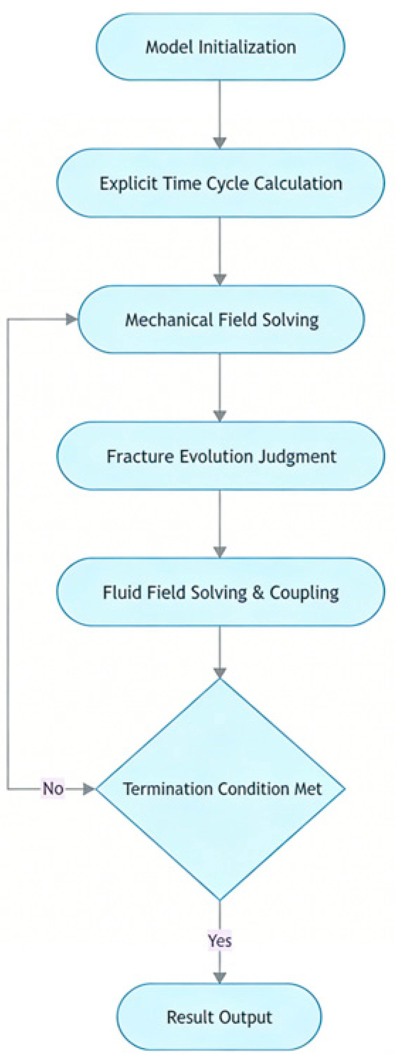
where ${\mathrm{w}}_0$ is the initial fracture width, and ${\mathrm{k}}_{\mathrm{n}}$ is the normal stiffness (Figure 1).

2.4. Physical Model

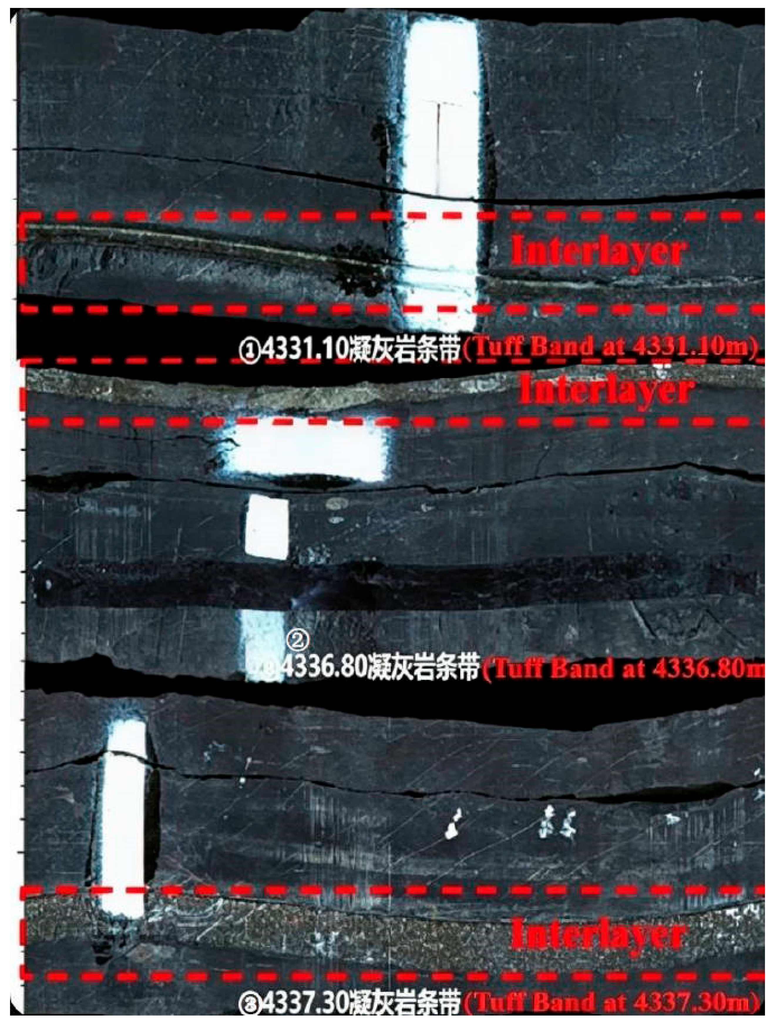
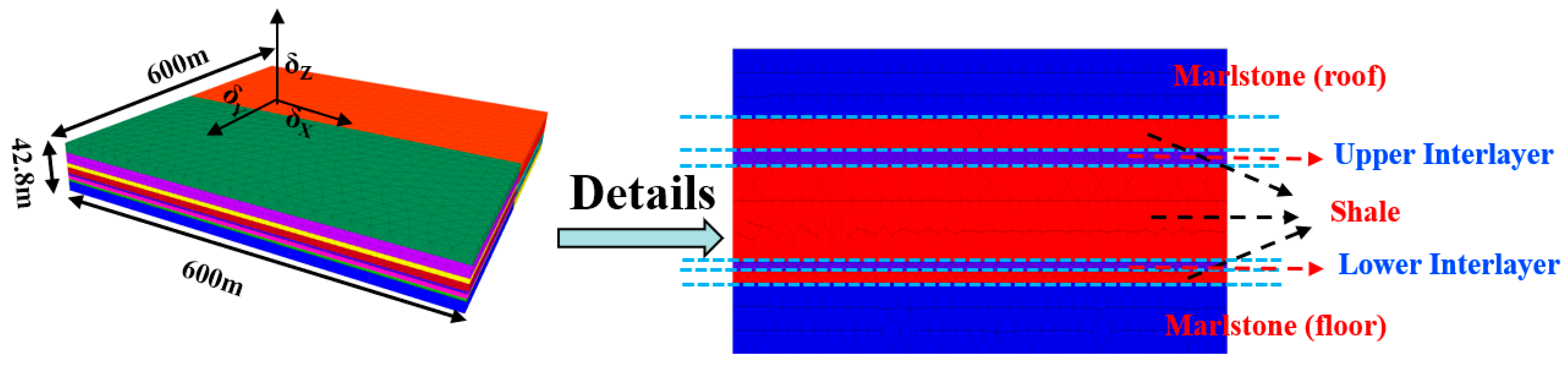
To explore the propagation laws of complex fracture networks in interbedded shale, a combined physical and numerical simulation approach was adopted to establish a model for simulating the propagation of complex fracture networks in interbedded shale and investigating the influence of different parameters on the propagation laws of complex fractures. The model is constructed based on the basic data of shale in the WJP Formation of Sichuan Province, consisting of several blocks (Figure 2). Based on the actual formation data studied in this paper, the model has a length, width, and height of 600 m, 600 m, and 42.8 m, respectively. In the model, the thickness of the roof and floor is 10 m each, where shale and interlayers are interleaved, including an upper interlayer and a lower interlayer. The specific structure and complete simulation parameters of the model are shown in Figure 3 and

Table 1. Schematic Table of Rock Structure Distribution in a Single Stage of a Field Fracturing Well.

Rock Type	Thickness (m)
Marlstone (roof)	10
Shale	4.1
Micritic limestone (interlayer)	2.5
Shale	13.1
Micritic limestone (interlayer)	1.4
Shale	1.7
Marlstone (floor)	10
Total	42.8

, and the input parameters are listed in

Table 2. Input parameters.

Shale		Interlayer		Roof and Floor		Fluid Properties
Parameter	Value	Parameter	Value	Parameter	Value	Parameter	Value
Young’s modulus E (GPa)	25	Young’s modulus E (GPa)	30	Young’s modulus E (GPa)	10	Fluid bulk modulus K (MPa)	3
Poisson’s ratio ν	0.2	Poisson’s ratio ν	0.24	Poisson’s ratio ν	0.25	Fluid density (kg/m3)	1000
Rock density (kg/m3)	2450	Rock density (kg/m3)	2650	Rock density (kg/m3)	2500	Fluid viscosity η (Pa·s)	0.0015
Rock tensile strength t (MPa)	2.5	Rock tensile strength t (MPa)	5	Rock tensile strength t (MPa)	2.5
normal stiffness kn (GPa)	10	normal stiffness kn (GPa)	15	normal stiffness kn (GPa)	5
shear stiffness ks (GPa)	7.5	normal stiffness kn (GPa)	15	normal stiffness kn (GPa)	5

.

To enhance the stability of the model’s grid structure and reduce the impact of grid division on simulation results, a refined meshing technique was used. Comparison between microseismic fracture monitoring data and simulation results shows that the influence of grid division on the results is negligible.

3. Model Validation

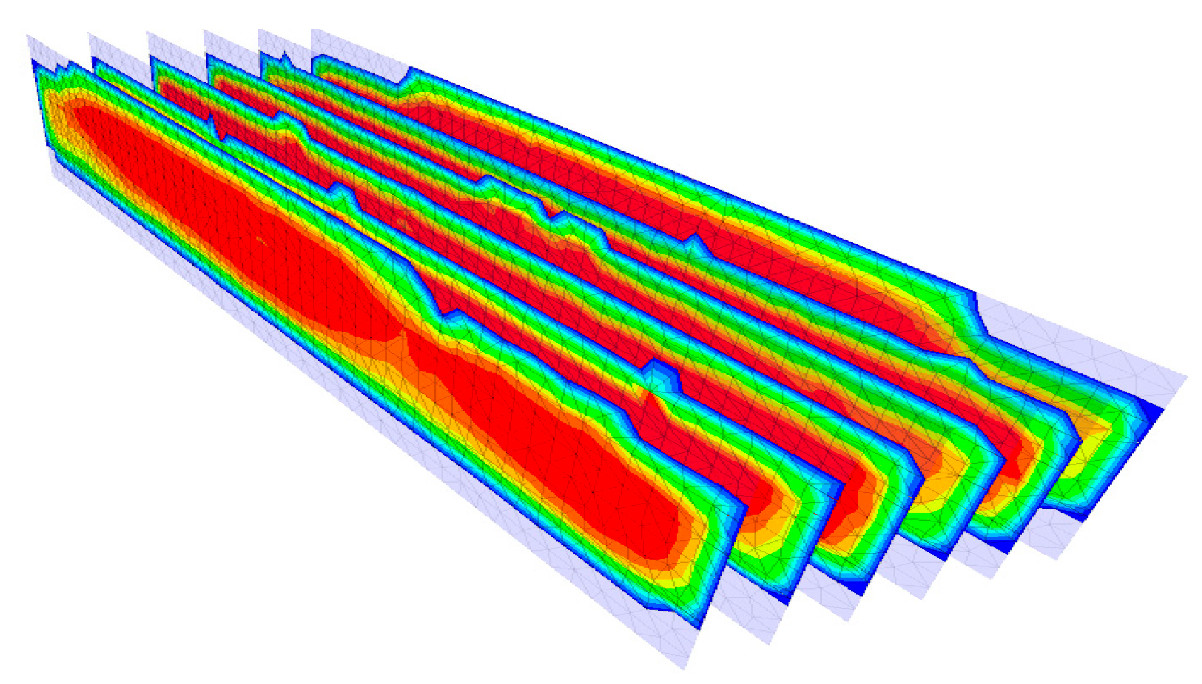
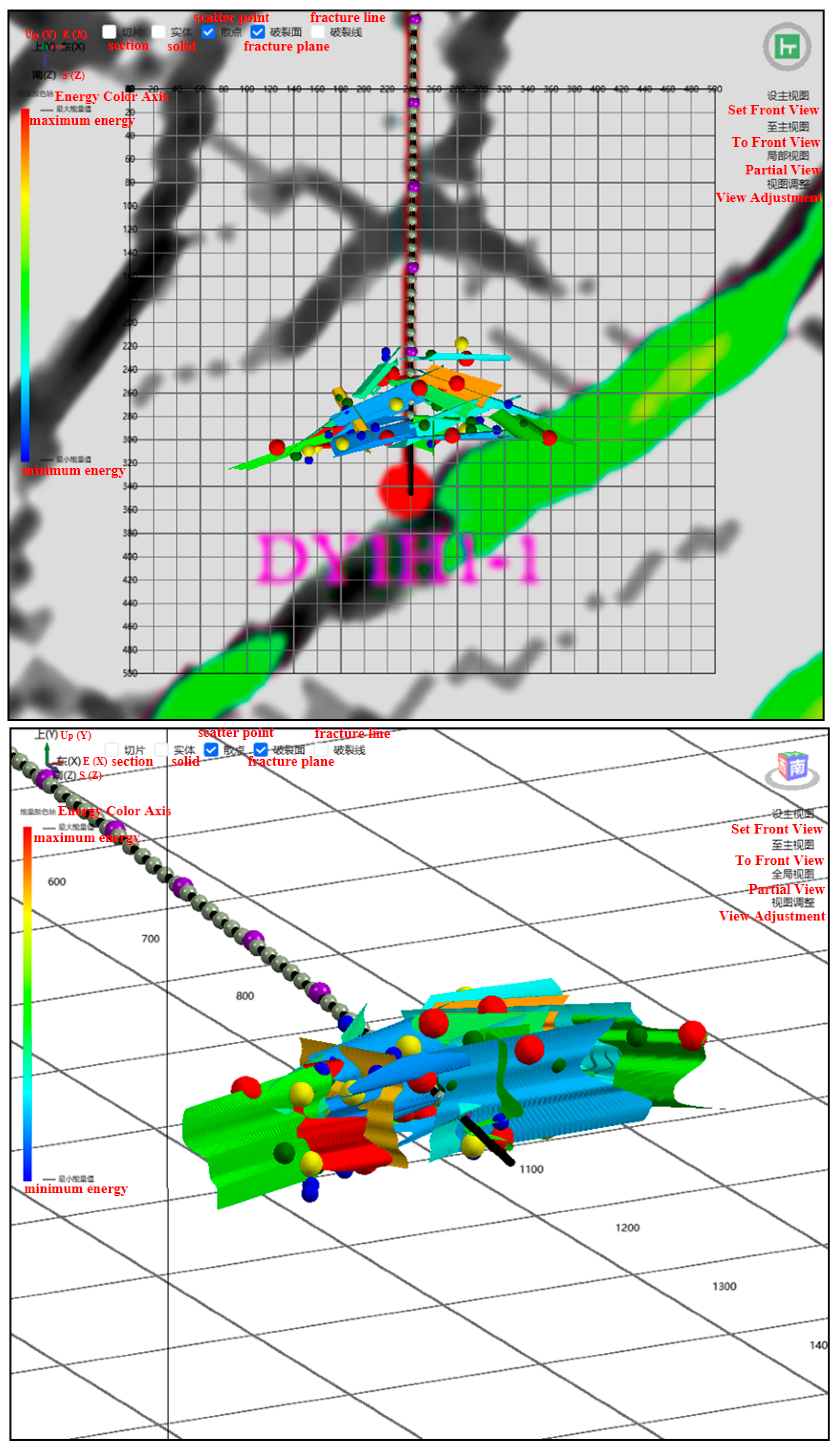
Field construction data from the main fracturing interval of the actual well are used to compare the simulation results (Figure 4 and Figure 5) with microseismic data (Figure 6). The fracture parameters from the simulation results correspond well to those from the fracture monitoring results (

Table 3. Comparison of fracture parameters between numerical simulation and microseismic monitoring.

Parameter	Fracture Length (m)	SRV (1 × 104 m3)
Microseismic monitoring (Interval 9 of Well Daye 1H1-2)	354	121.25
Numerical simulation (Interval 9 of Well Daye 1H1-2)	348	116.8

), verifying the reliability of the model. SRV (Stimulated Reservoir Volume) is the rock volume formed by hydraulic fracturing in ultra-low permeability reservoirs that is effectively connected by a complex fracture network, and it directly determines the drainage capacity and initial production of unconventional oil and gas [29]. The calculation method for SRV originates from the numerical simulation study on hydraulic fracture propagation in coalbed methane considering coal seam cleats by Xiao et al. [30] based on the three-dimensional discrete element method.

4. Results and Discussion

4.1. Effects of Reservoir Parameters

4.1.1. Horizontal Stress Difference

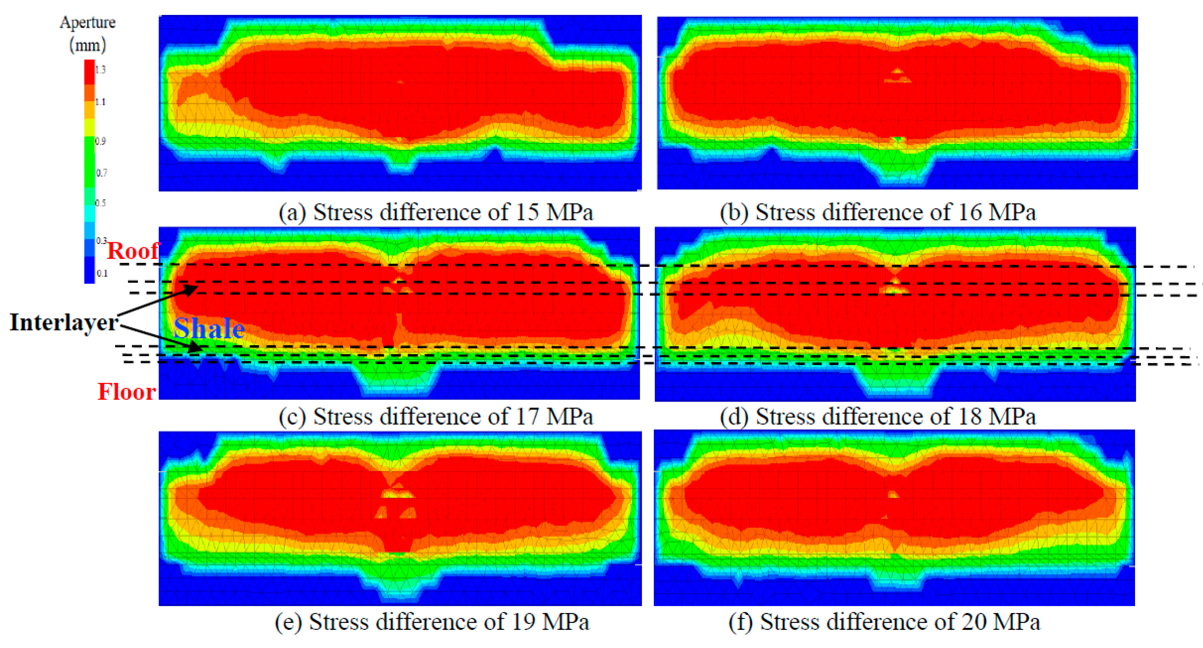
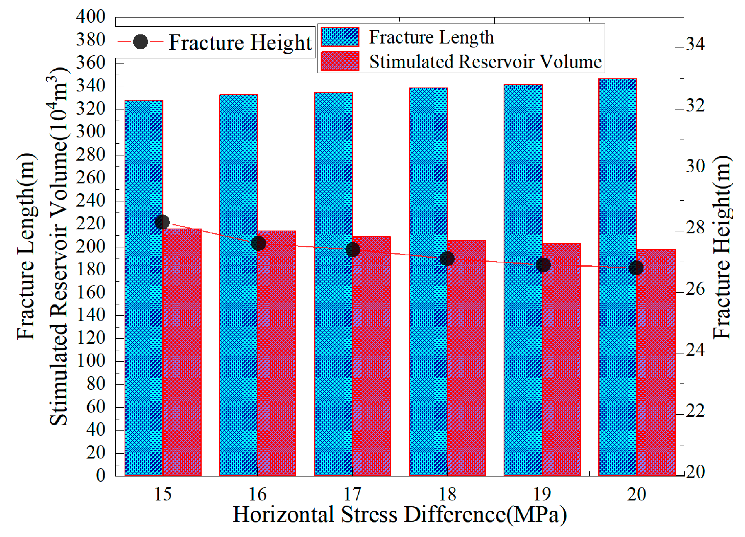
When the stress difference increases from 15 MPa to 20 MPa, the fracture height gradually decreases from 28.3 m to 26.8 m, with a decrease amplitude of approximately 5% (Figure 7 and Figure 8). During this process, no fracture penetration through interlayers occurs, and vertical propagation is continuously inhibited with the increase in stress difference, with the propagation speed gradually slowing down. This is because the increase in stress difference enhances the horizontal stress constraint, limiting the vertical expansion of fractures and making it difficult for the fracture height to increase. When the stress difference changes within the reservoir range, the fracture height can break through the upper interlayer of the reservoir, but it is difficult to break through the lower interlayer due to its high limestone content. This finding is consistent with the research conclusions of Chang X [31] et al. The greater the stress difference, the stronger the suppression of barriers/interlayers on the vertical propagation of fractures, making it more difficult for fracture height to grow and for fractures to penetrate layers.

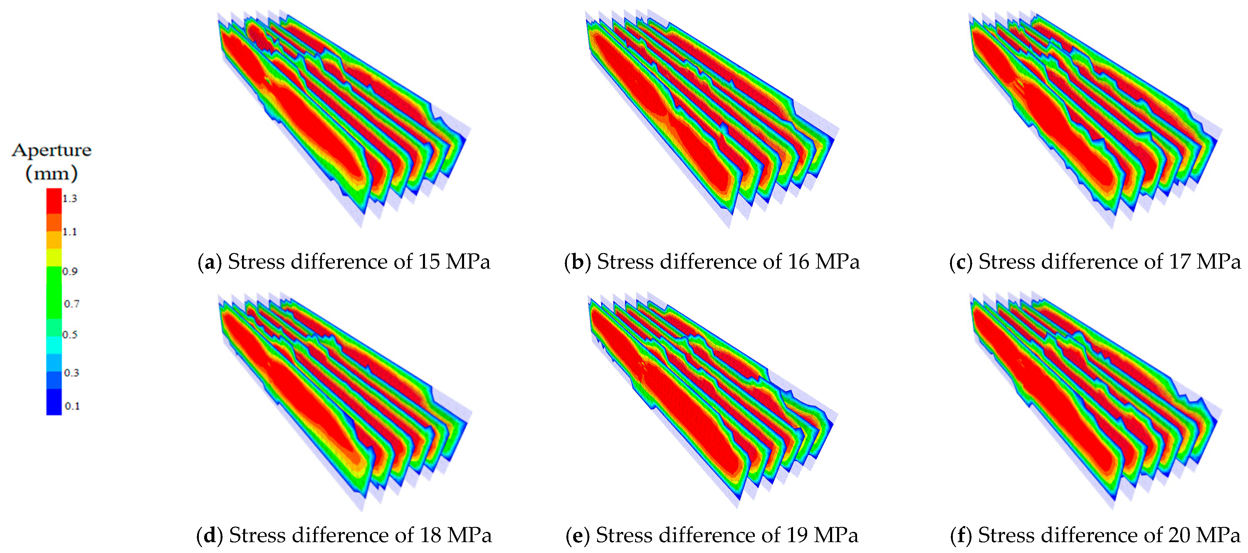
The fracture length continues to increase with the increase in stress difference (328 m → 347 m) (Figure 8 and Figure 9), and the propagation speed gradually accelerates. This is because the increase in horizontal stress difference provides a stronger guiding effect for the lateral extension of fractures; however, the stimulated reservoir volume (SRV) decreases with the increase in stress difference, indicating that a high stress difference can promote fracture “lengthening” but is not conducive to the formation of complex fracture networks, resulting in a reduction in the overall stimulation range.

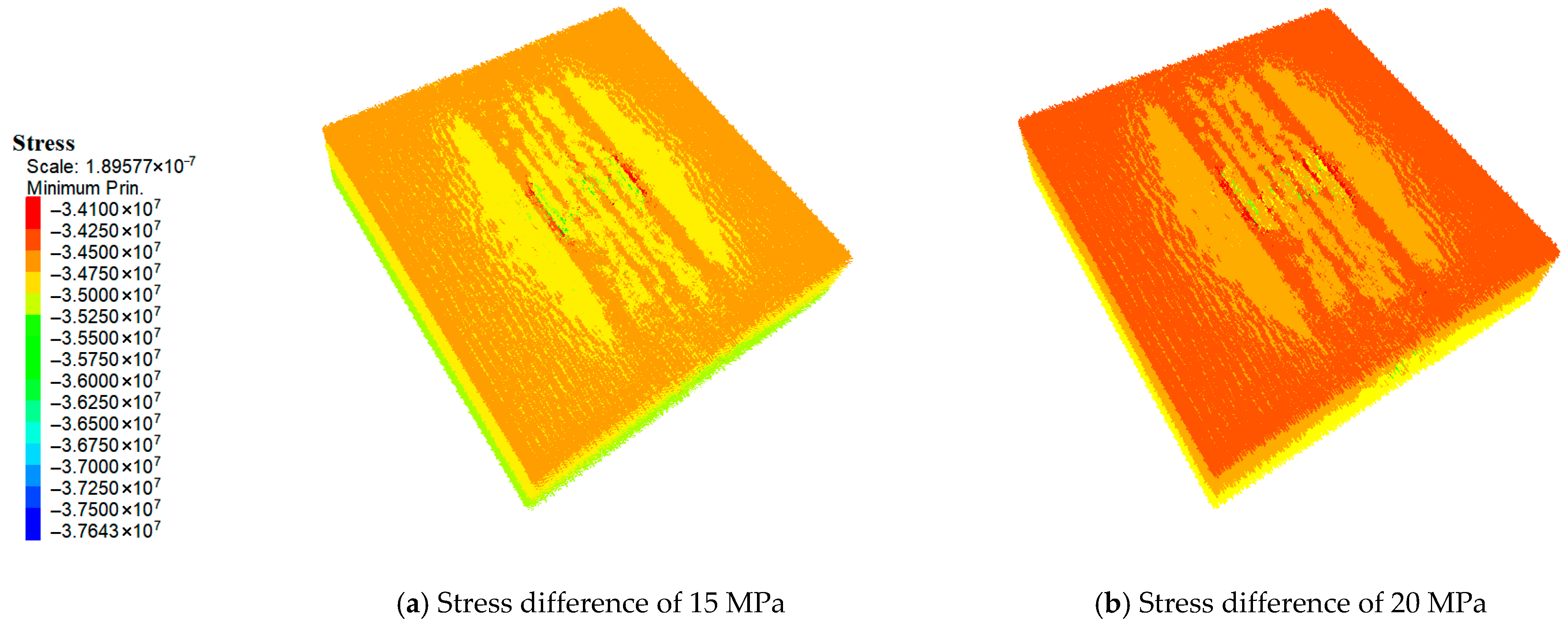
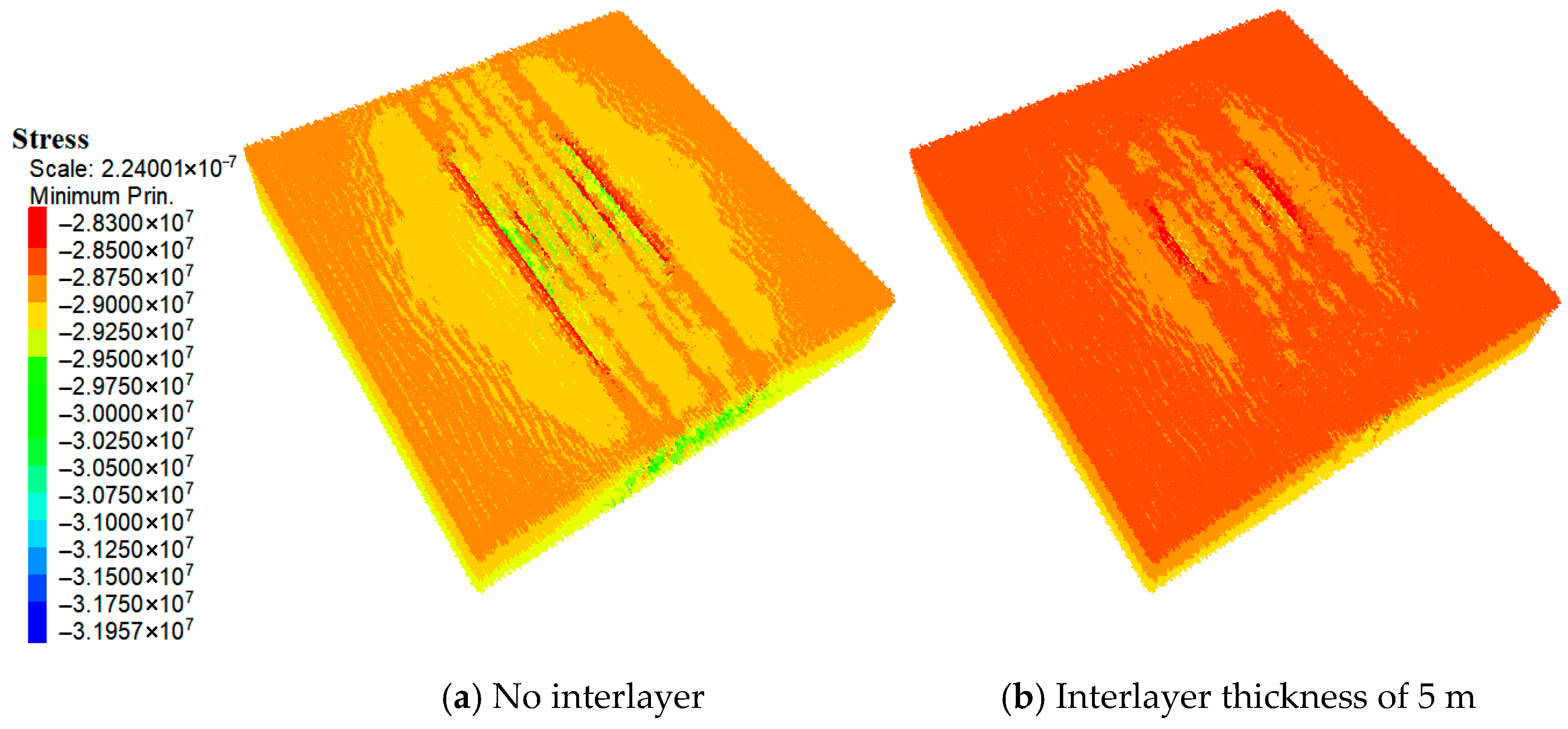
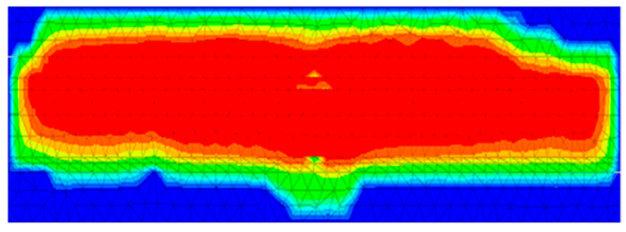
When the stress difference increases from 15 MPa to 20 MPa, the vertical propagation of fractures remains continuously suppressed and fails to penetrate the interlayer (Figure 10). The central area of the reservoir is preferentially penetrated by fractures, after which the stress difference in this zone decreases accordingly, thus forming a stress distribution characterized by a smaller stress difference in the central region and a larger stress difference in the surrounding areas. The upper and lower interlayers with high stress differences impose strong vertical constraints on fractures, and only under low stress difference conditions can fractures penetrate the upper interlayer.

4.1.2. Influence of Interlayer Thickness on Hydraulic Fractures

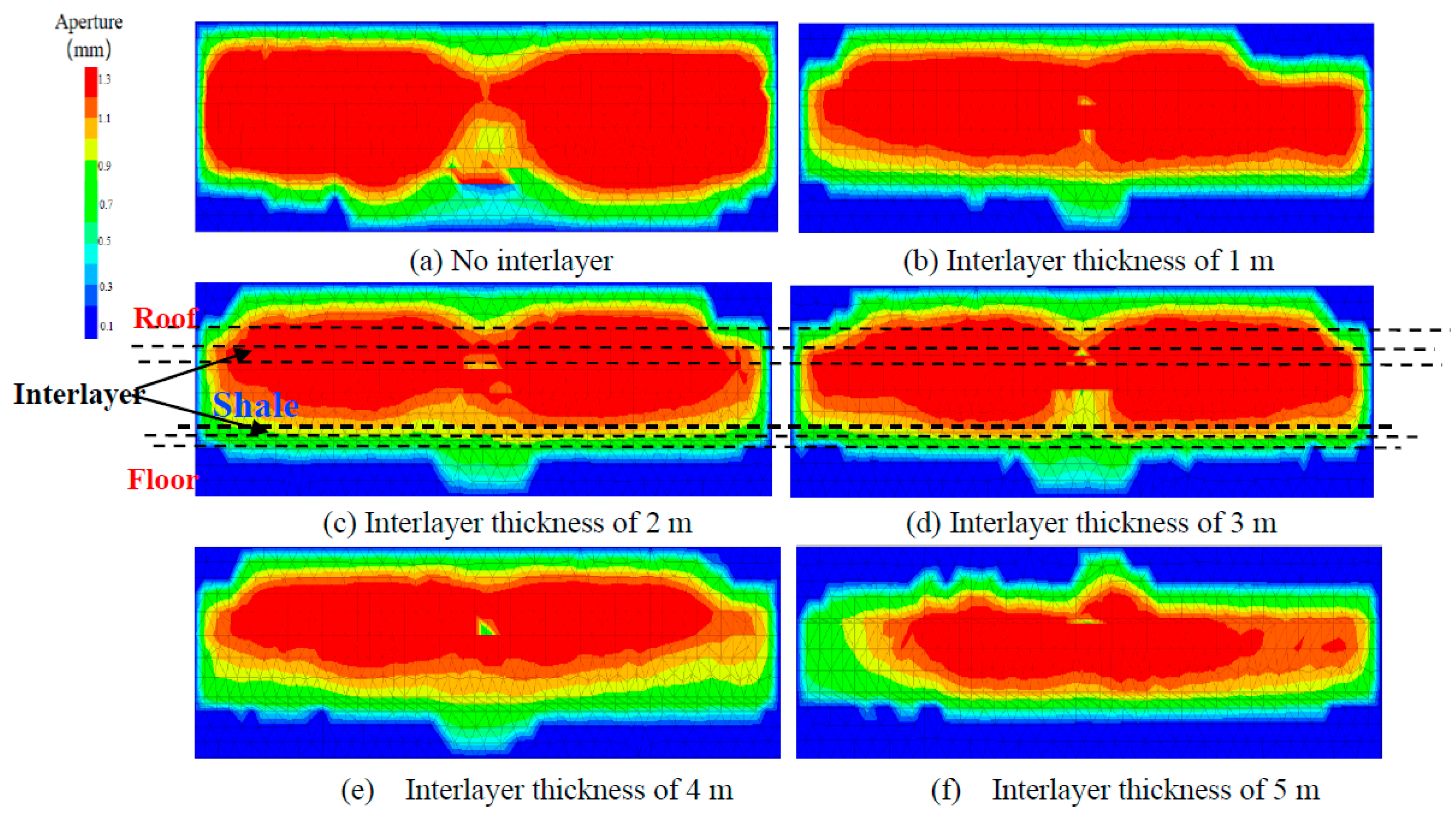
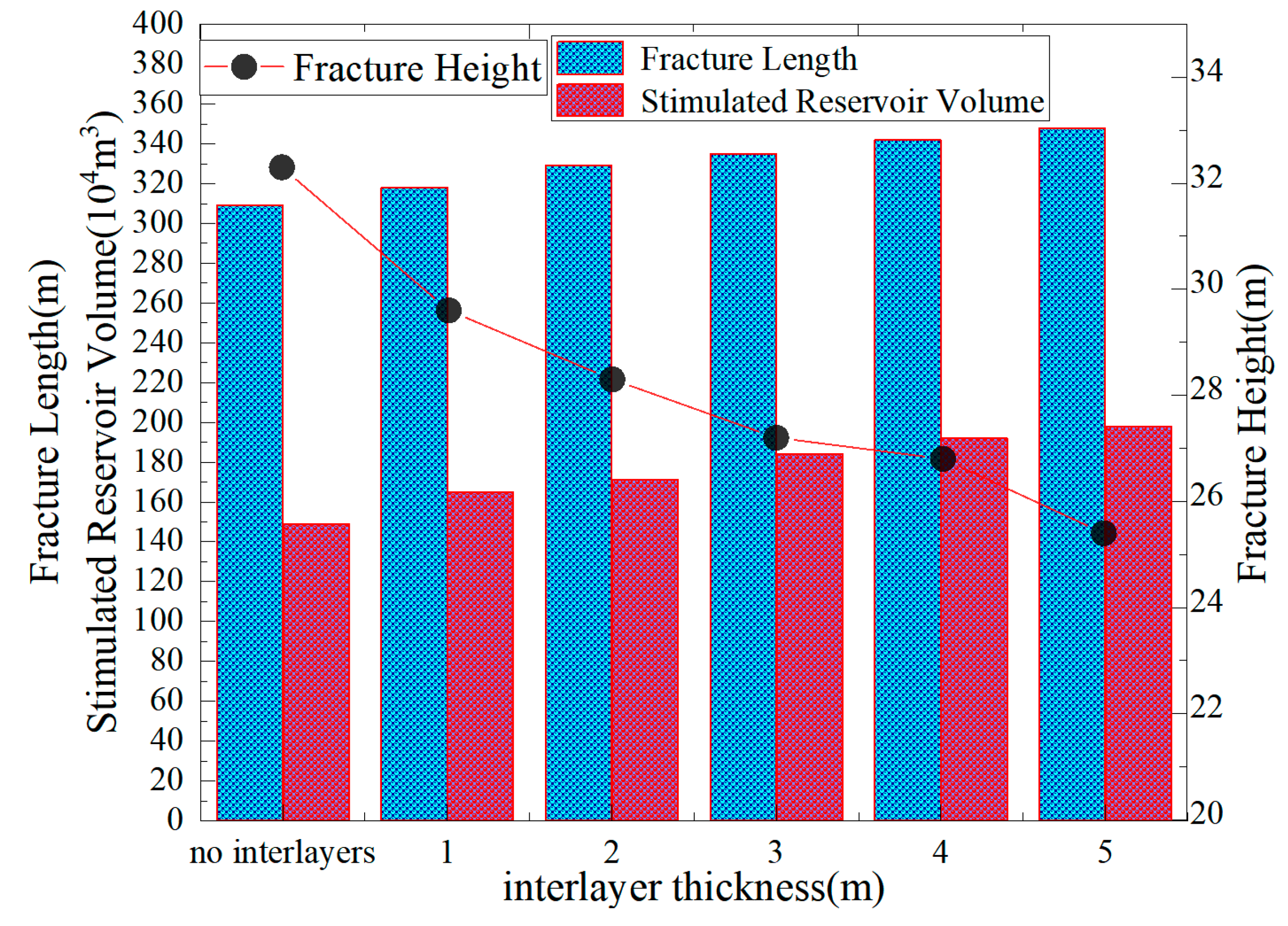
The fracture height is the largest when there are no interlayers in the formation; as the interlayer thickness increases from 1 m to 5 m, the fracture height decreases significantly (32.3 m → 25.4 m), with a decrease amplitude of approximately 21% (Figure 11 and Figure 12). After the increase in interlayer thickness, it is difficult for fractures to penetrate the hard interlayer rock, and the vertical propagation speed continues to slow down, without breaking through the interlayer into the upper or lower reservoirs. As a physical barrier, the interlayer directly hinders the vertical extension of fractures, and the thicker the interlayer, the stronger the hindering effect.

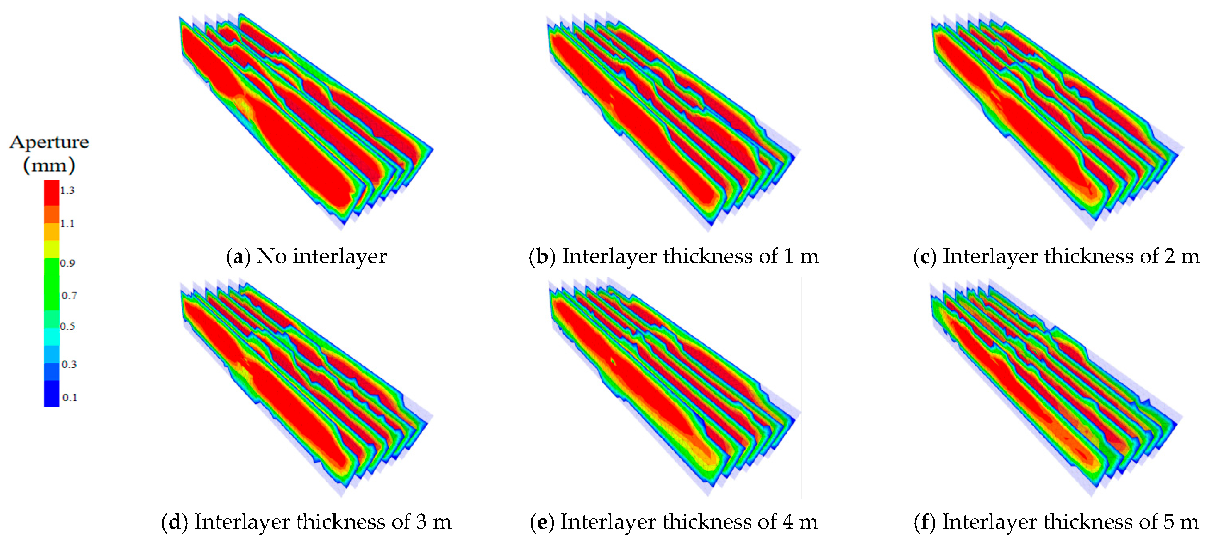
Due to the presence of upper and lower interlayers in shale reservoirs, these interlayers act as barriers that prevent the fracturing fluid from breaking through and propagating upward or downward during hydraulic fracturing. As a result, the fracture length exhibits a slowly increasing trend with greater interlayer thickness. In the absence of interlayers, the fracture length is the shortest (approximately 309 m), whereas when the interlayer thickness increases to 5 m, the fracture length correspondingly extends to 348 m. Compared to the case without interlayers, the increase in fracture length is approximately 13%, indicating that the promotion of fracture length by increasing interlayer thickness is relatively moderate. The stimulated reservoir volume (SRV) also increases significantly with increasing interlayer thickness. The SRV is minimal when no interlayers are present and reaches its maximum value when the interlayer thickness attains 5 m (Figure 12 and Figure 13).

After fracture breakthrough occurs in the central area of the reservoir, the stress difference in the corresponding zone decreases accordingly, forming a distribution pattern of low stress difference in the central area and high stress difference in the surrounding area (Figure 14). When the condition changes from no interlayer to an interlayer with a thickness of 5 m, the interlayer forms a strong stress barrier, which significantly inhibits the vertical propagation of fractures.

4.2. Effects of Engineering Parameters on Hydraulic Fractures

4.2.1. Influence of Pumping Rate on Hydraulic Fractures

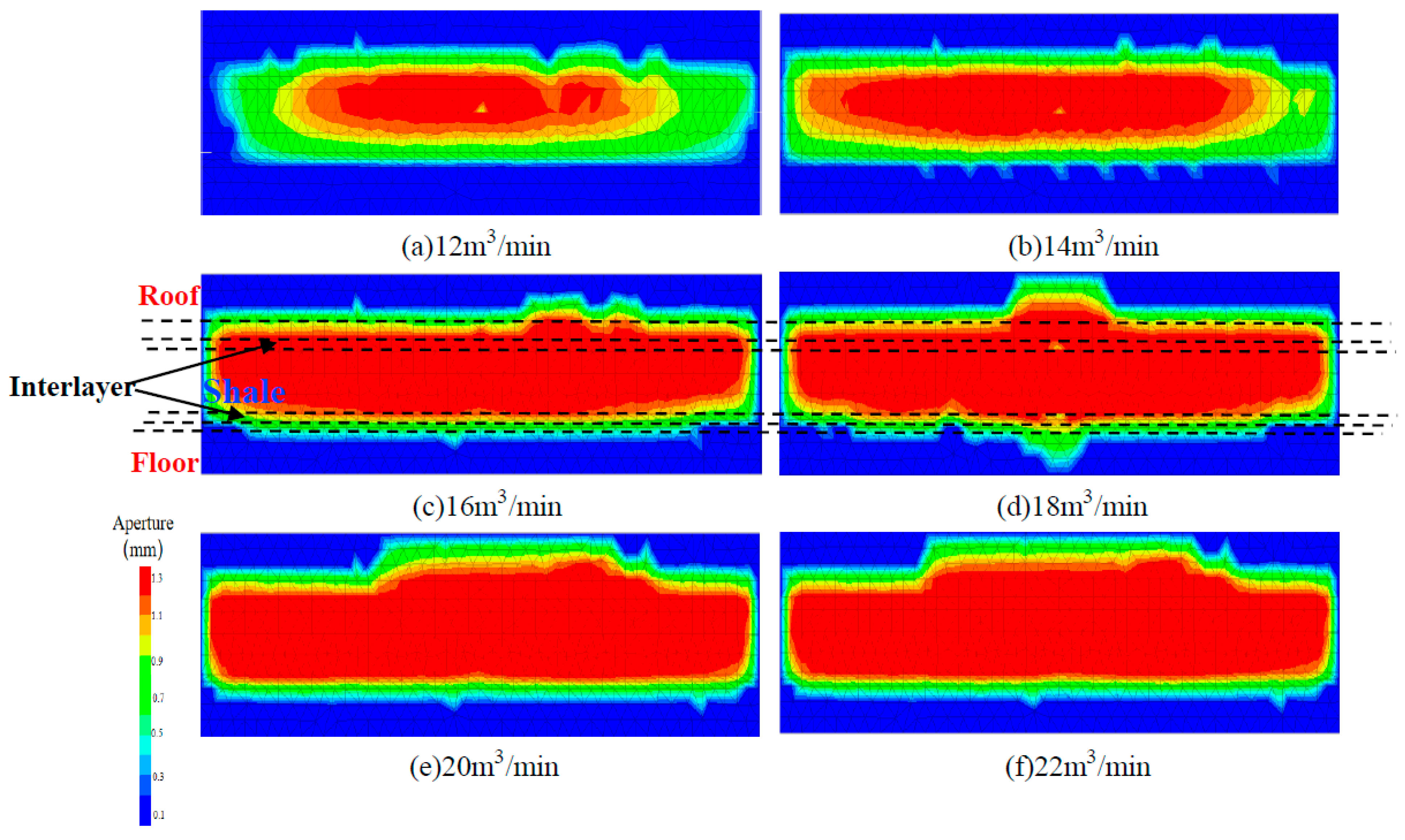
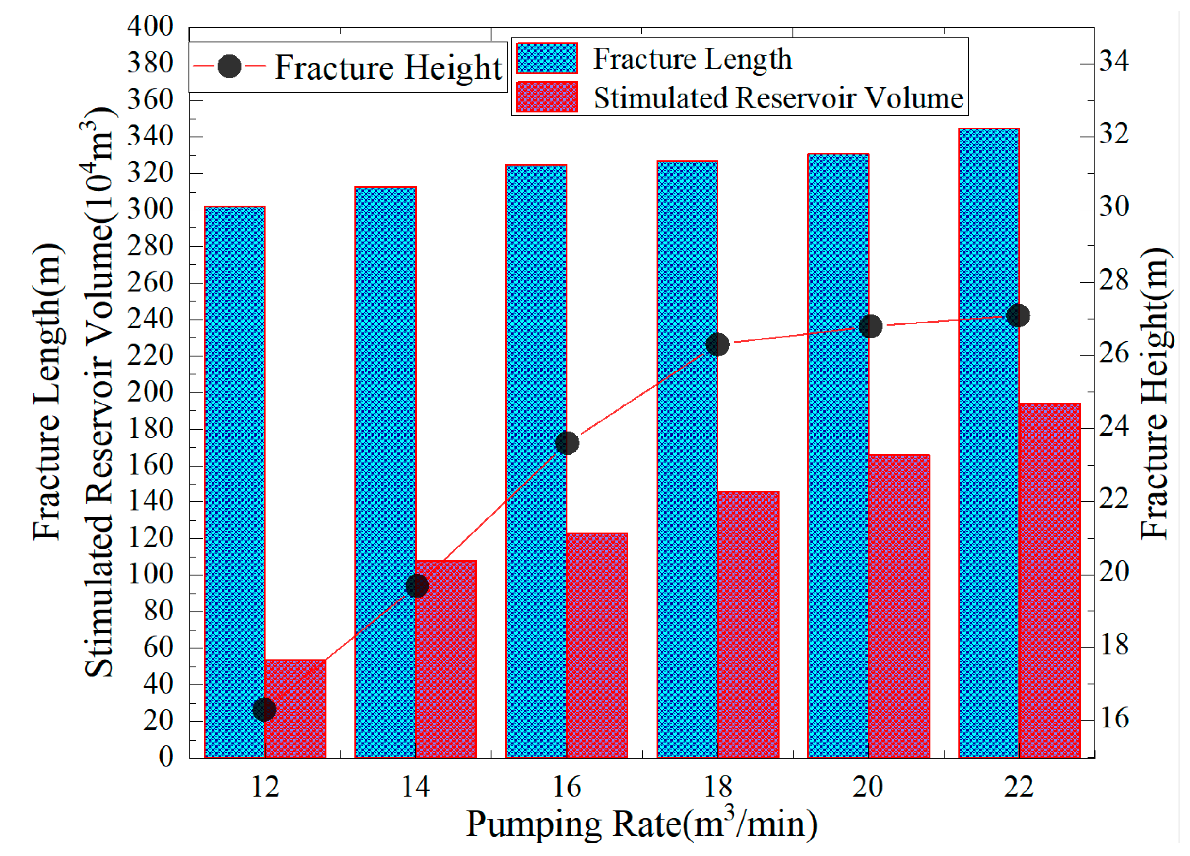
When the pumping rate gradually increases from 12 m³/min to 22 m³/min, the fracture height shows a characteristic of “rapid growth first and then stabilization”. In the range of 12–16 m³/min, the fracture height significantly increases from 16.3 m to 27.1 m. During this stage, the rapid accumulation of fracture energy successfully breaks through the calcareous interlayer in the upper part of the reservoir, and the vertical propagation speed increases significantly; when the pumping rate exceeds 16 m³/min, the growth rate of fracture height slows down significantly. When the pumping rate is between 18 m³/min and 22 m³/min, the fracture height only fluctuates slightly between 26.36 and 27.1 m, approaching a stable value (Figure 15 and Figure 16). This is due to the enhanced vertical stress constraint of the formation and the balanced distribution of fluid pressure in the fracture, resulting in insufficient vertical propagation power and significantly increased difficulty in breaking through deeper interlayers.

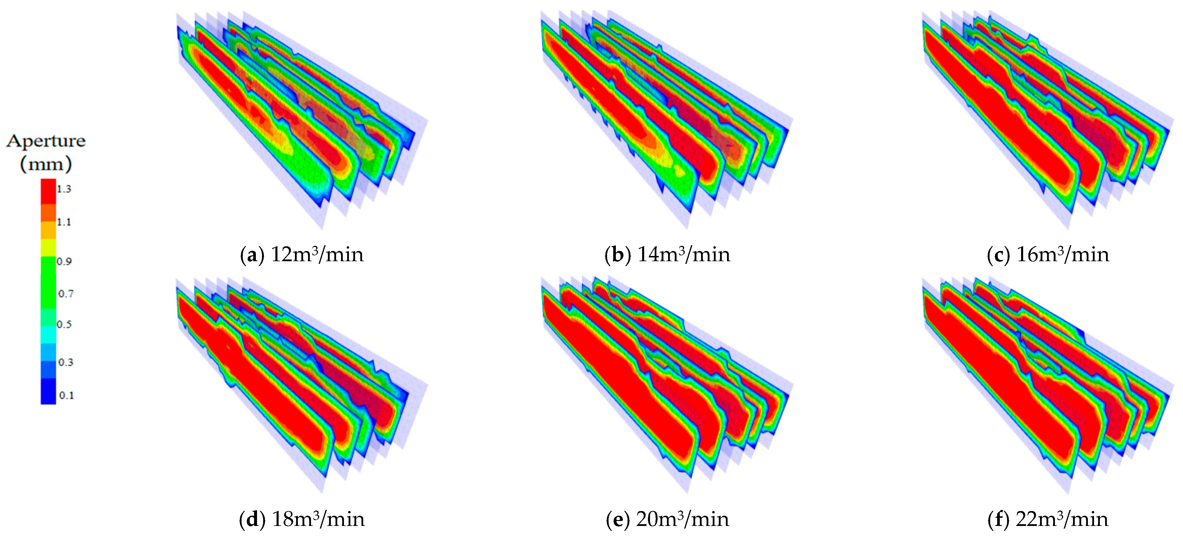
The influence of pumping rate on fracture length and SRV shows a continuous positive correlation trend (Figure 16 and Figure 17). The fracture length steadily increases with the increase in pumping rate: approximately 190 m at 12 m³/min and 360 m at 22 m³/min, with an overall increase amplitude of 89%, indicating that a higher pumping rate can provide stronger power for the lateral extension of fractures, promoting the rapid extension of fractures to longer distances. The stimulated reservoir volume (SRV) shows an approximately linear growth relationship with the pumping rate, increasing from approximately 81 × 10⁴ m³ at 12 m³/min to 345 × 10⁴ m³ at 22 m³/min, with an increase amplitude of over 326%. This indicates that the increase in pumping rate not only increases the fracture length but also significantly expands the formation stimulation range by enhancing the branching and connectivity of the fracture network.

4.2.2. Influence of Fluid Volume on Hydraulic Fractures

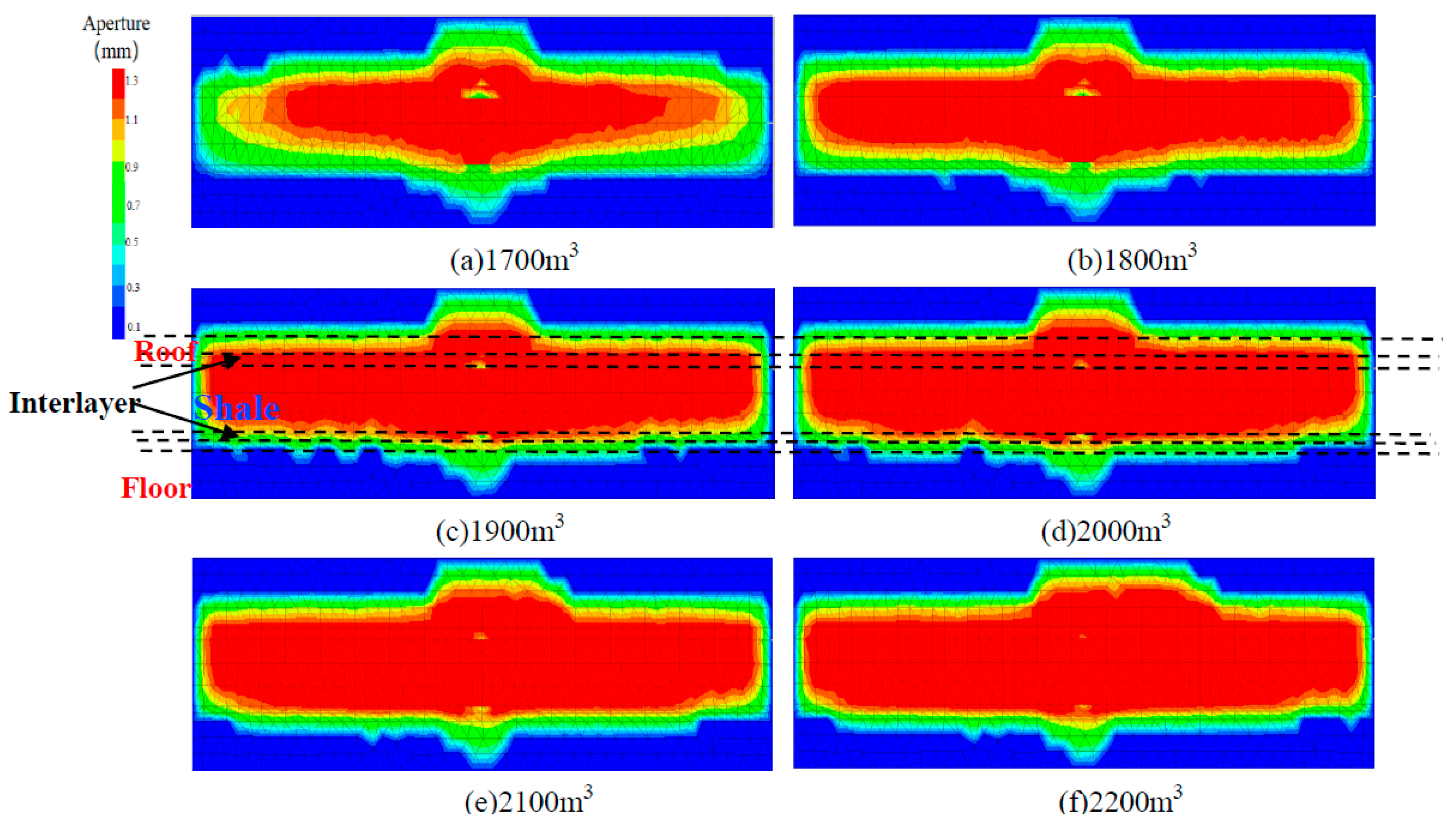
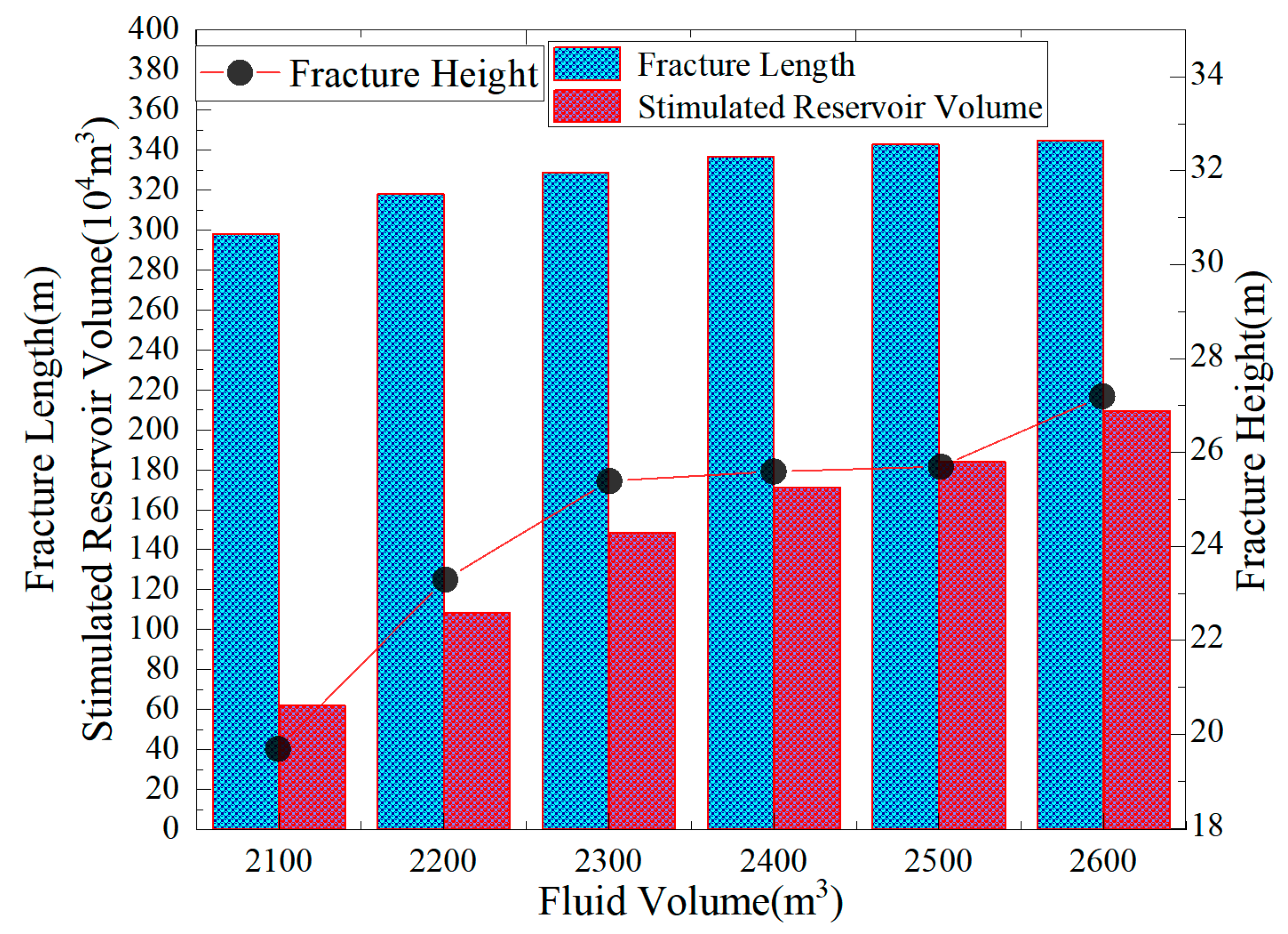
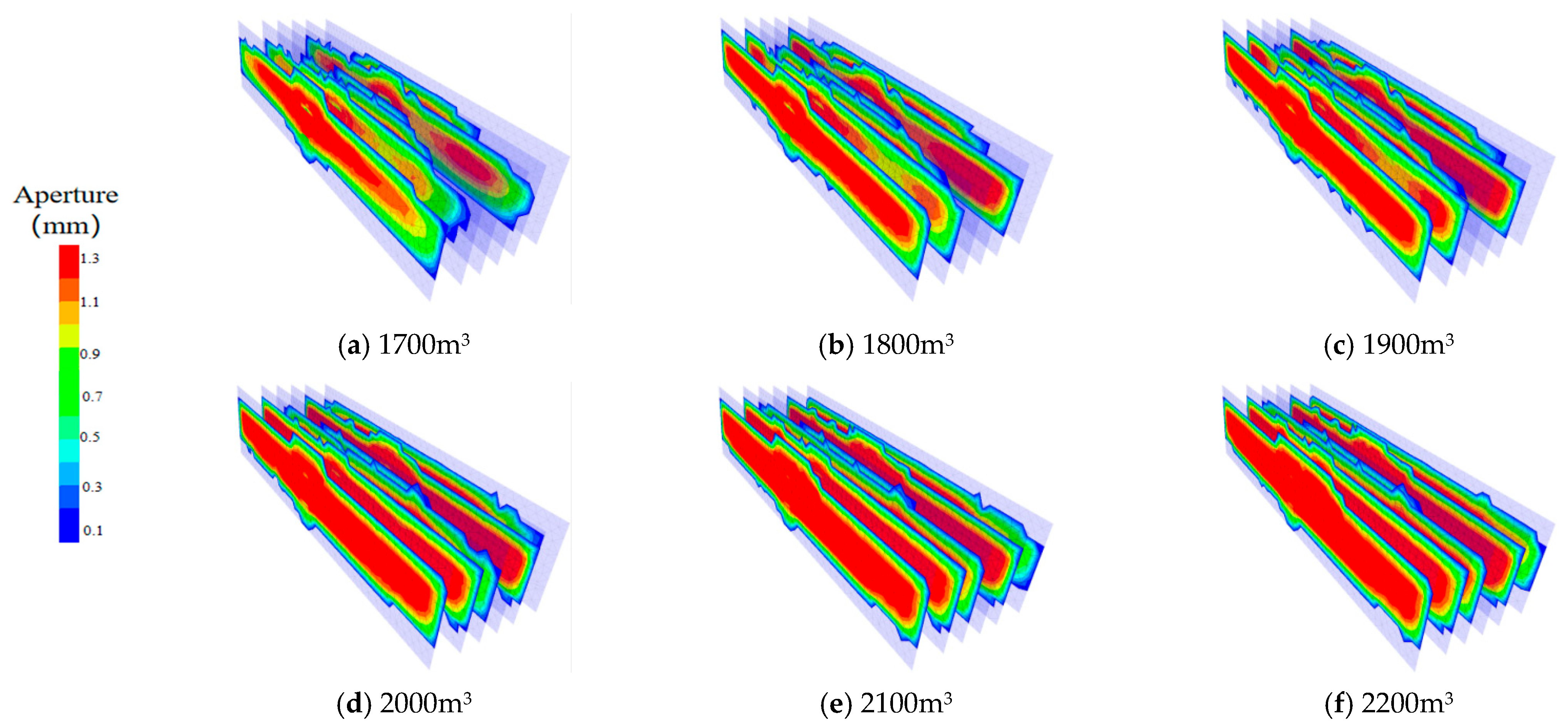
In the range of 1700–2200 m³, the fracture height shows a trend of “rapid growth first and then slowing down” with the increase in fluid volume. When the fluid volume increases from 1700 m³ to 1900 m³, the fracture height increases from 19.7 m to 25.4 m (Figure 18 and Figure 19). During this stage, the continuous accumulation of fluid volume provides sufficient energy for the vertical propagation of fractures, successfully breaking through the calcareous interlayer in the middle of the reservoir, and the vertical propagation speed increases significantly; when the fluid volume exceeds 1900 m³, the growth of fracture height tends to be gentle, indicating that there is a threshold for the promoting effect of fluid volume on fracture height. Beyond the threshold, the vertical stress of the formation and the pressure in the fracture reach a balance, and the vertical propagation is limited, with the speed significantly slowing down.

The influence of fluid volume on fracture length and SRV has significant phased characteristics (Figure 19 and Figure 20). The fracture length grows rapidly when the fluid volume is 1700–2000 m³: from approximately 280 m to 345 m, with an increase amplitude of approximately 23%; when the fluid volume exceeds 2000 m³, the growth rate of fracture length slows down, maintaining around 343 m at 2200 m³, indicating that the fluid volume needs to reach a certain threshold to provide sufficient power for fracture length extension, but excessive fluid volume has limited gain on fracture length. The stimulated reservoir volume (SRV) shows a trend of “first increasing and then stabilizing” with the increase in fluid volume: approximately 180 × 10⁴ m³ at 1700 m³, reaching 360 × 10⁴ m³ at 2000 m³ (an increase amplitude of 100%), and slightly decreasing to 343 × 10⁴ m³ at 2200 m³. This indicates that a reasonable fluid volume can expand the fracture network through continuous fluid injection, but excessive fluid volume may lead to increased fluid loss and reduced efficiency, resulting in stagnant or slightly decreased SRV growth.

4.2.3. Influence of Viscosity on Hydraulic Fractures

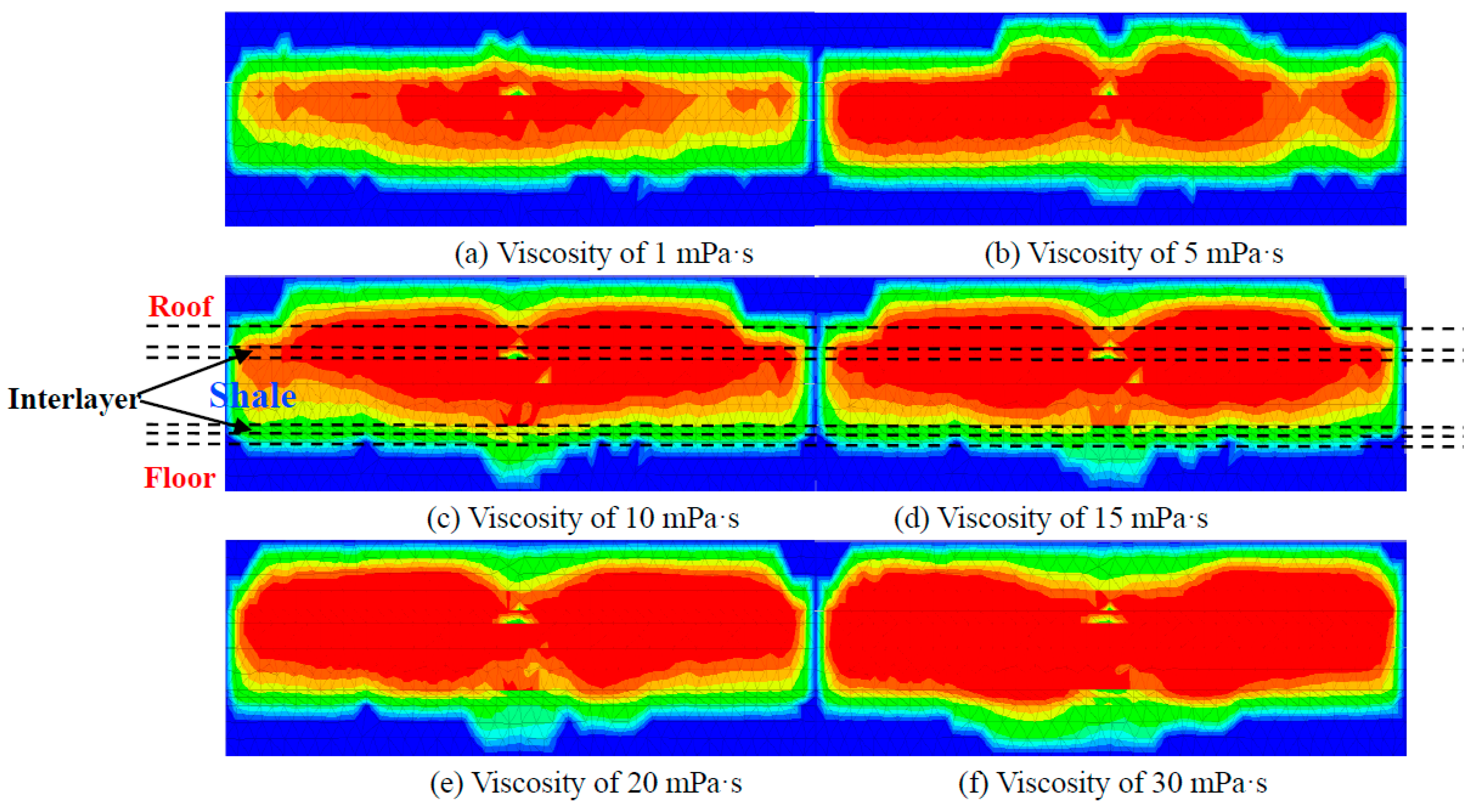
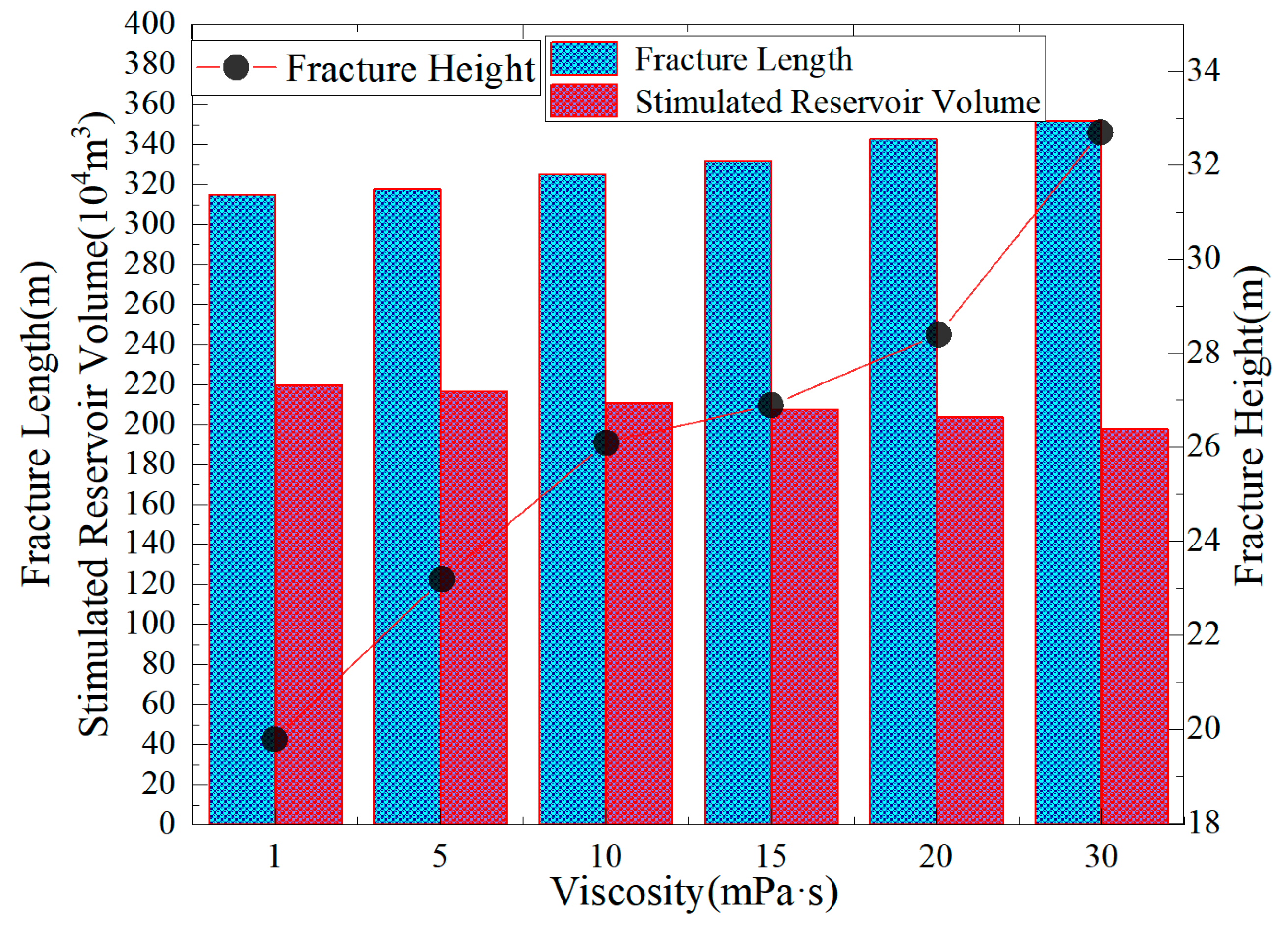
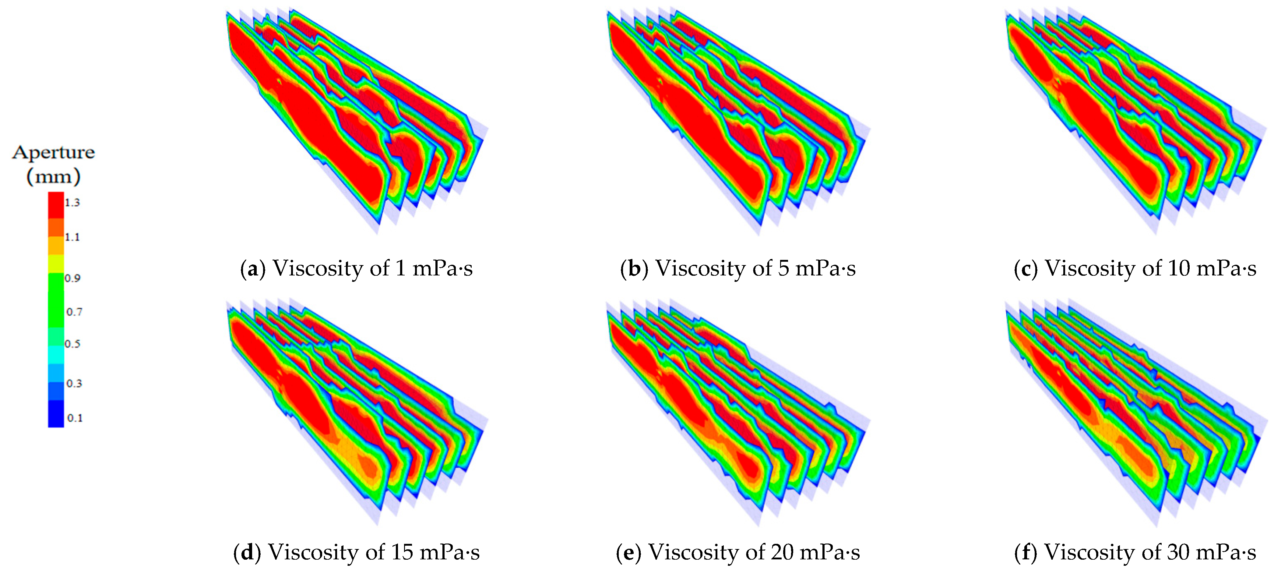
Viscosity shows a significant positive correlation with the hydraulic fracture height. When the fluid viscosity is 1 mPa·s, the fracture height reaches the minimum value of 19.8 m (Figure 21 and Figure 22). At this time, although the low-viscosity fluid has strong fluidity, its proppant-carrying capacity is weak, and the pressure is easily dispersed in the reservoir, making it difficult to form a stable supporting force to promote the vertical breakthrough of fractures. The calcareous interlayer in the upper part of the reservoir significantly restricts fracture propagation, and the vertical propagation speed is slow.

With the gradual increase in fluid viscosity (from 5 mPa·s to 30 mPa·s), the fracture height shows a continuous upward trend, increasing from 23.2 m to 32.7 m, with an overall increase amplitude of approximately 65%. The proppant-carrying performance of high-viscosity fluid increases synchronously with viscosity, and the pressure transmission is more concentrated, which is not easy to disperse and lose. It can effectively overcome the interlayer resistance, providing stable support for the vertical propagation of fractures, making the vertical propagation speed of fractures continuously accelerate; especially when the viscosity exceeds 20 mPa·s, the upward trend of fracture height is more prominent. This phenomenon fully indicates that high-viscosity fluid has a significant promoting effect on the vertical propagation of fractures.

The fracture length increases slightly with the increase in viscosity: approximately 315 m at 1 mPa·s and 343 m at 30 mPa·s, with an increase amplitude of approximately 9% (Figure 22 and Figure 23). This is because high-viscosity fluid can maintain higher pressure in the fracture, promoting the slow lateral extension of fractures. However, the stimulated reservoir volume (SRV) is larger at low viscosity: 360 × 10⁴ m³ at 1 mPa·s and 315 × 10⁴ m³ at 30 mPa·s, with a decrease amplitude of approximately 13%, indicating that low viscosity is conducive to the disorderly propagation of fractures to form complex fracture networks (with many branches and good connectivity), while high viscosity can extend the fracture length but inhibits fracture branching, resulting in a simple fracture network and a reduced overall stimulation volume.

4.3. Effects of Perforation Parameters on Hydraulic Fractures

4.3.1. Influence of Number of Clusters on Hydraulic Fractures

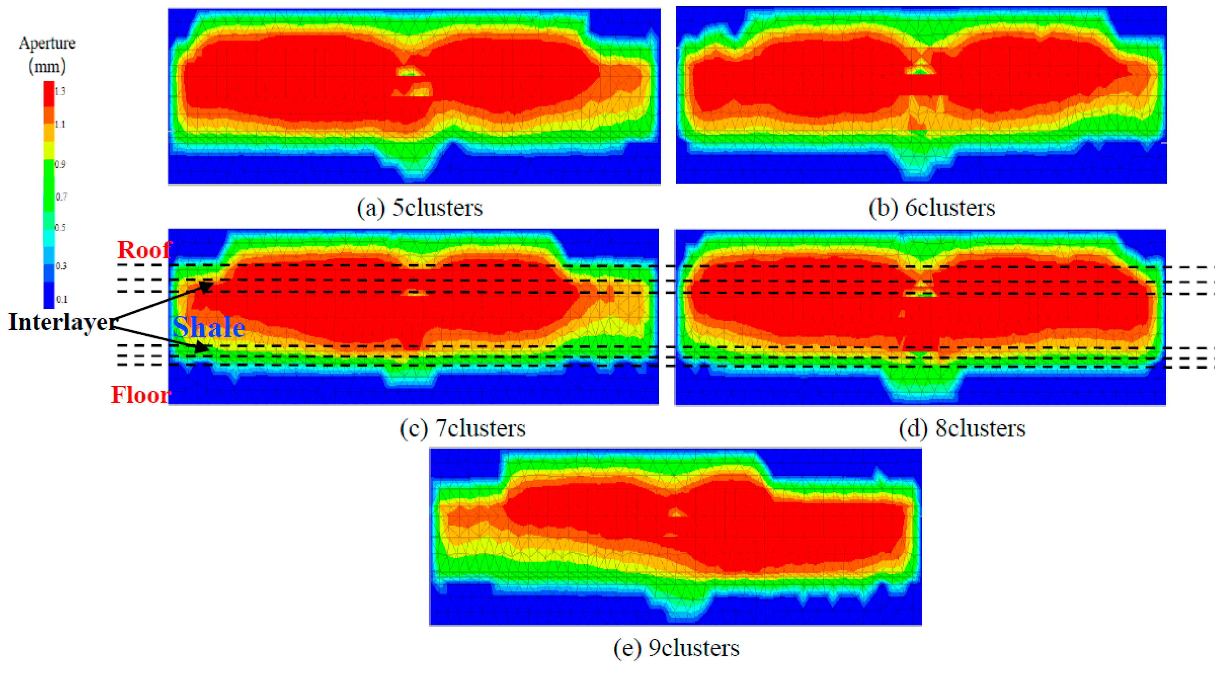
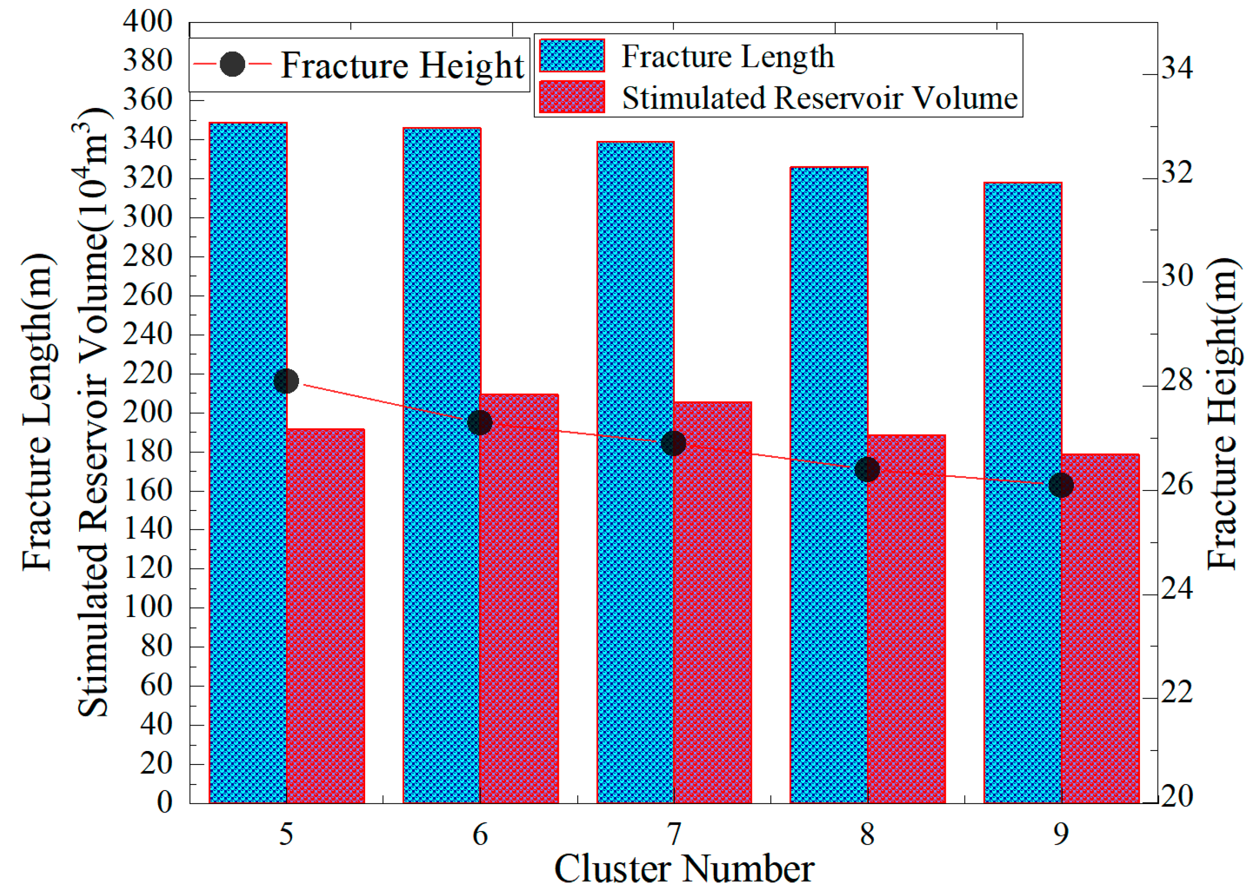
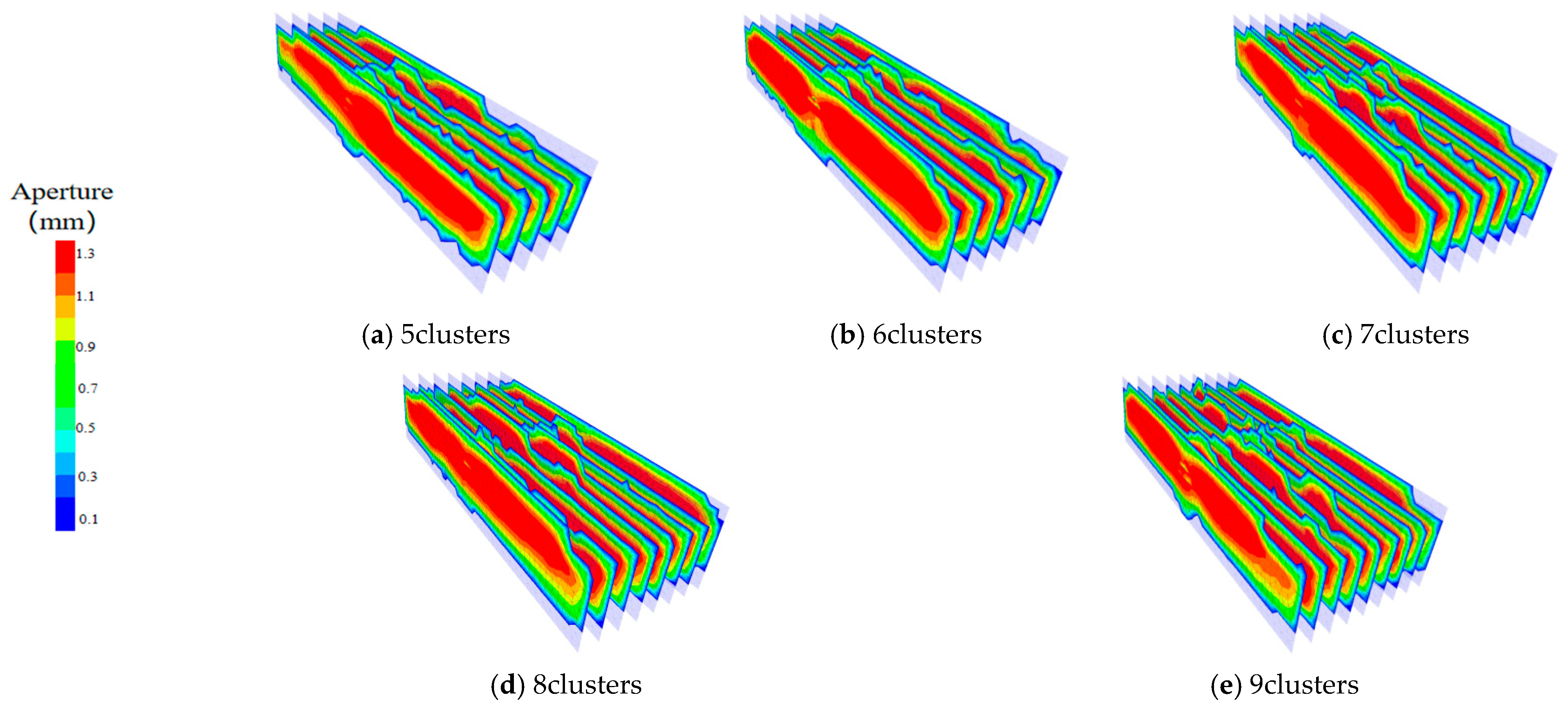
The influence of the number of clusters on fracture height shows a trend of “stabilization first and then decrease”: the fracture height is the largest (28.1 m) when the number of clusters is 5 (Figure 24 and Figure 25). At this time, the energy obtained by a single cluster is concentrated, and the fracture is easy to break through the upper and lower interlayers of the reservoir, with a fast vertical propagation speed; as the number of clusters increases to 9, the fracture height decreases slightly to 26.1 m, with a decrease amplitude of approximately 7%. The distribution of multiple clusters leads to energy dispersion, and the pressure of a single cluster is insufficient to quickly break through the interlayer, with the vertical propagation speed gradually slowing down. Especially when the number of clusters exceeds 7, the downward trend of fracture height is more obvious, indicating that an excessive number of clusters will weaken the vertical breakthrough capacity of a single cluster. When the number of clusters is small, the energy of fracturing fluid is concentrated in a single cluster, the fracture extension resistance is small, and it can break through the upper interlayer of the Daye reservoir, resulting in a longer single fracture length. With the increase in the number of clusters, the fracture length and height decrease slightly. When the number of clusters is 6–7, the fracture is difficult to break through the interlayer, and the stimulated reservoir volume increases to the maximum and then decreases.

The fracture length fluctuates slightly with the increase in the number of clusters: approximately 326 m at 5 clusters, increasing to 349 m at 7 clusters, and slightly decreasing to 346 m at 9 clusters, with an overall variation amplitude of approximately 6% (Figure 25 and Figure 26). The stimulated reservoir volume (SRV) reaches a peak when the number of clusters is 6–7. At this time, the number of clusters is moderate, which can not only ensure a certain degree of energy concentration (avoiding excessive dispersion) but also form a more complex fracture network through multi-cluster synergy; when the number of clusters increases to 9, the SRV decreases slightly due to excessive energy dispersion leading to a reduction in the stimulation range of a single cluster and a decrease in the overall connectivity of the fracture network.

4.3.2. Influence of Cluster Spacing on Hydraulic Fractures

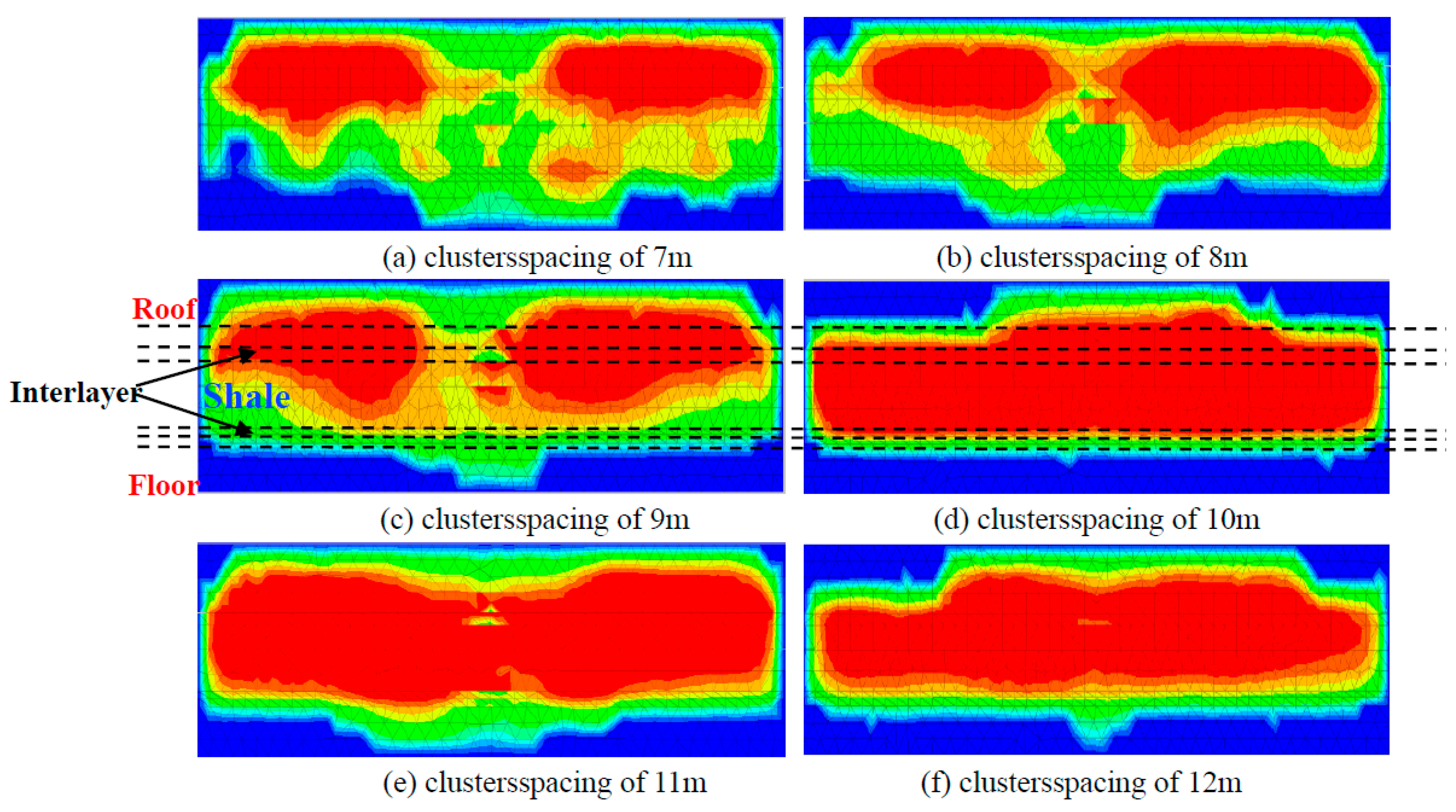
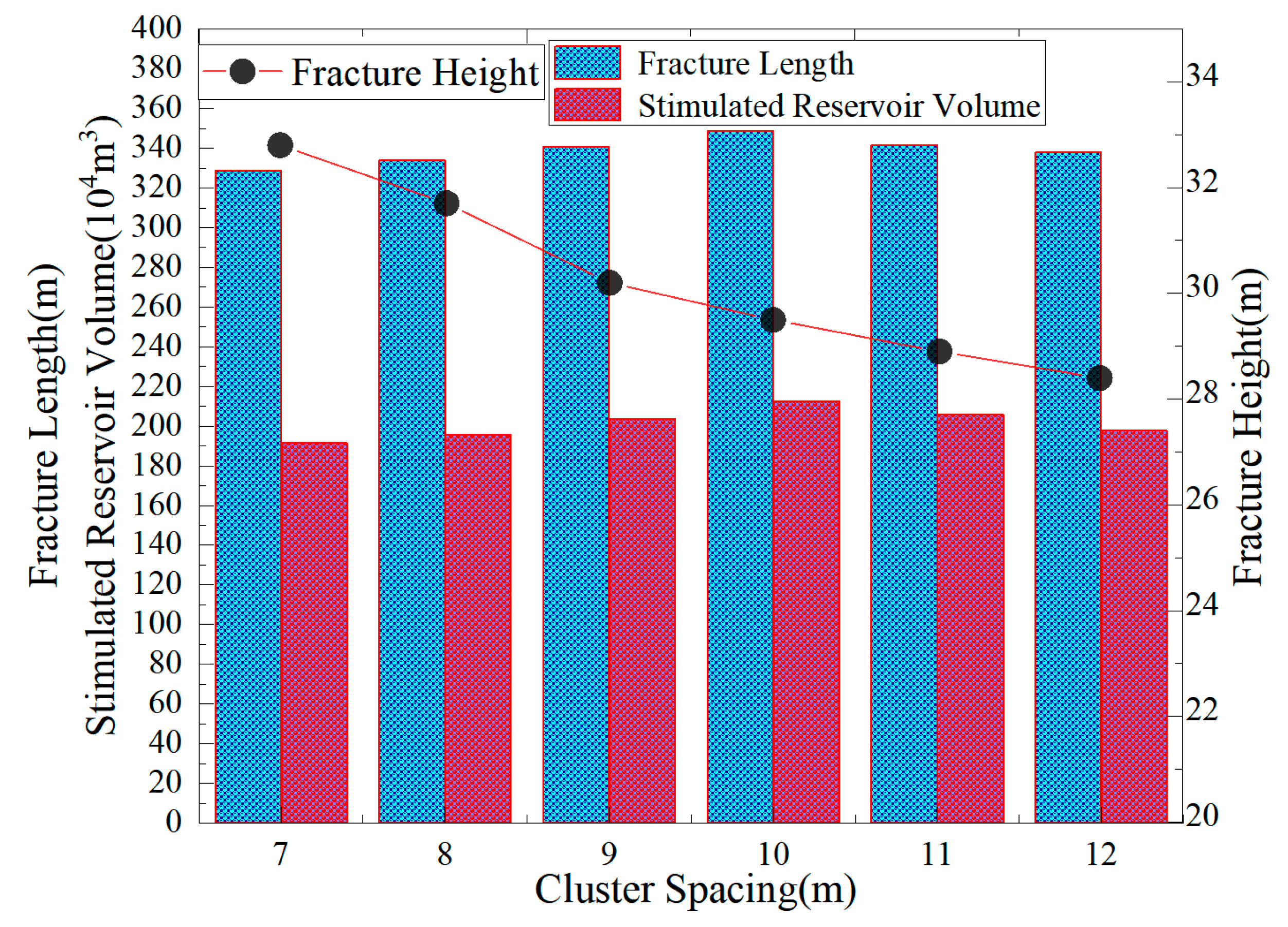
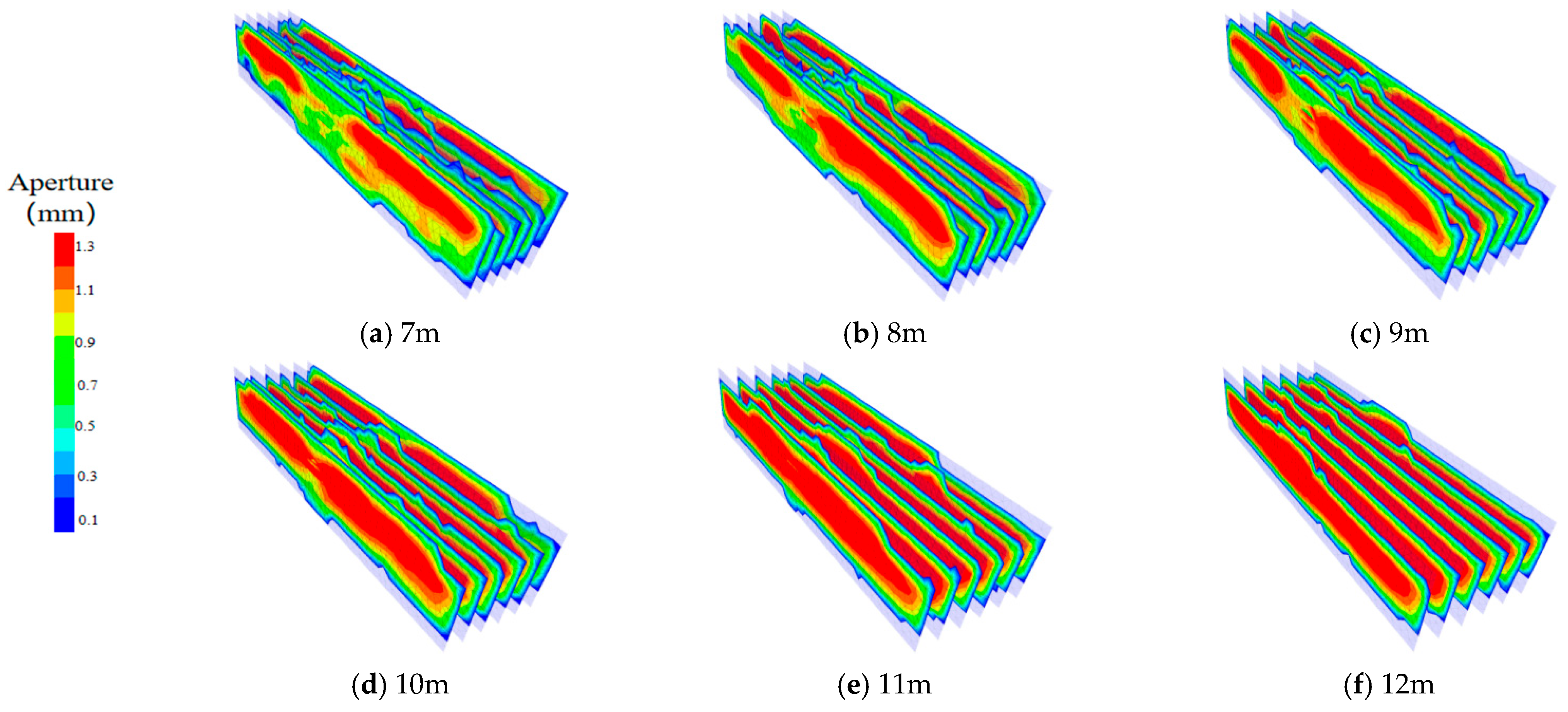
The influence of cluster spacing on fracture height shows a trend of “decrease first and then stabilization”: the fracture height is the largest (32.8 m) when the cluster spacing is 7 m. At this time, the relatively small spacing leads to strong stress interference, the fracture propagation of the middle cluster is inhibited, and the edge clusters obtain more energy, which is easy to break through the interlayer, with a fast vertical propagation speed; as the spacing increases to 12 m, the fracture height gradually decreases to 28.4 m, with a decrease amplitude of approximately 13% (Figure 27 and Figure 28). The stress interference weakens, and the energy distribution of a single cluster is more uniform, but the power to break through the interlayer is weakened, and the vertical propagation speed gradually slows down. Especially when the spacing exceeds 10 m, the downward trend of fracture height slows down, indicating that the vertical propagation of fractures is more stable but less capable under larger spacing. When the cluster spacing is small, the stress interference increases, the fracture propagation of the middle cluster is inhibited, the fracture length, width, and stimulated reservoir volume all decrease, and the interlayer is more likely to be broken through, leading to an increase in fracture height; when the cluster spacing increases to 10 m, the stress interference decreases, the fracture length increases, and the stimulated reservoir volume reaches the maximum.

Both the fracture length and SRV reach the maximum when the cluster spacing is 10 m: fracture length of 342 m and SRV of 341 × 10⁴ m³ (Figure 28 and Figure 29). At this time, the spacing is moderate, the stress interference is minimal, and a single cluster can not only expand fully but also form a complex fracture network through moderate synergy; when the spacing is too small (7 m), the excessive stress interference leads to shortened fracture length of some clusters and overlapping fracture networks; when the spacing is too large (12 m), the synergy between clusters weakens, and the connectivity of the fracture network decreases, so both the fracture length and SRV are lower than those at a spacing of 10 m.

4.3.3. Influence of Perforation Location on Hydraulic Fractures

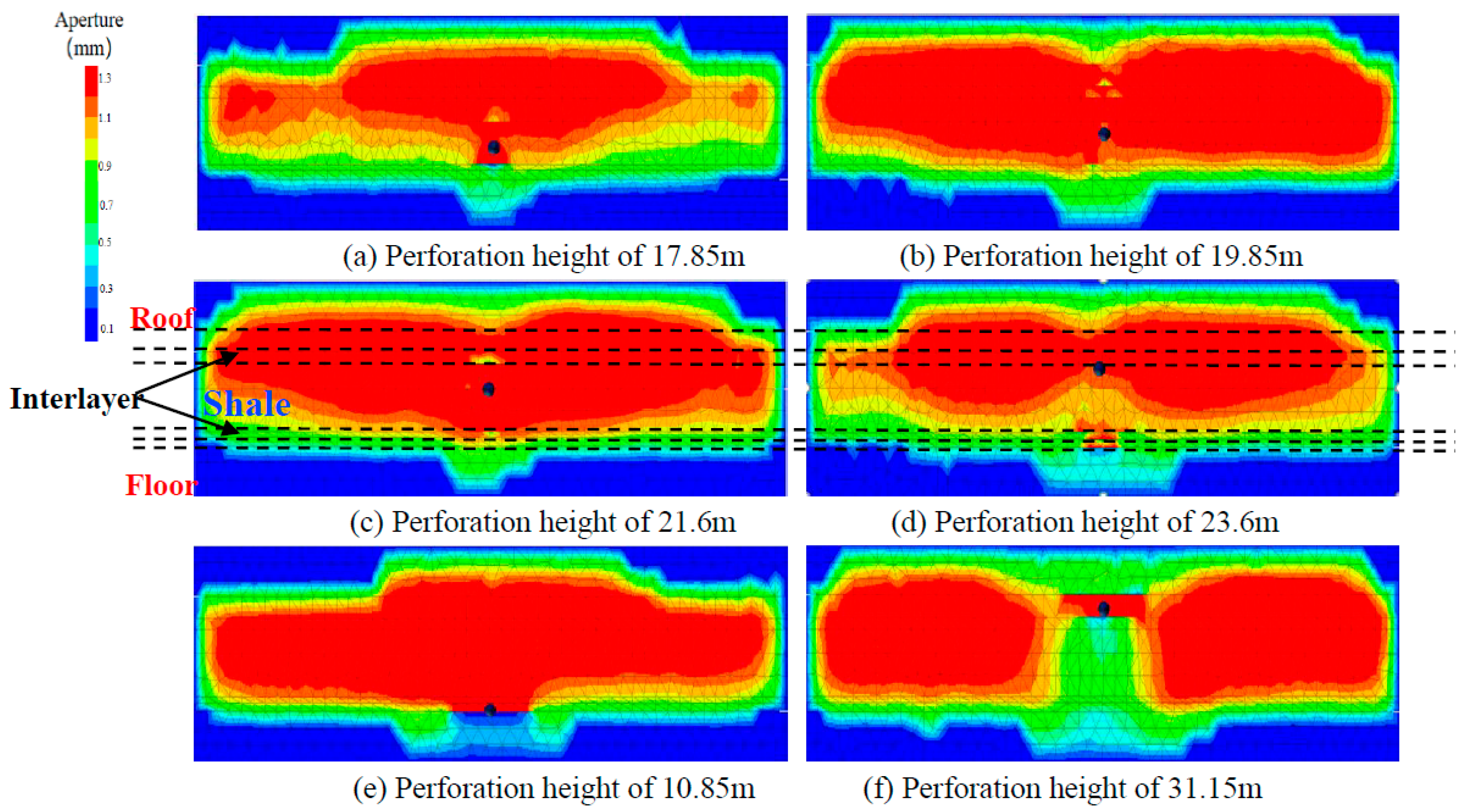
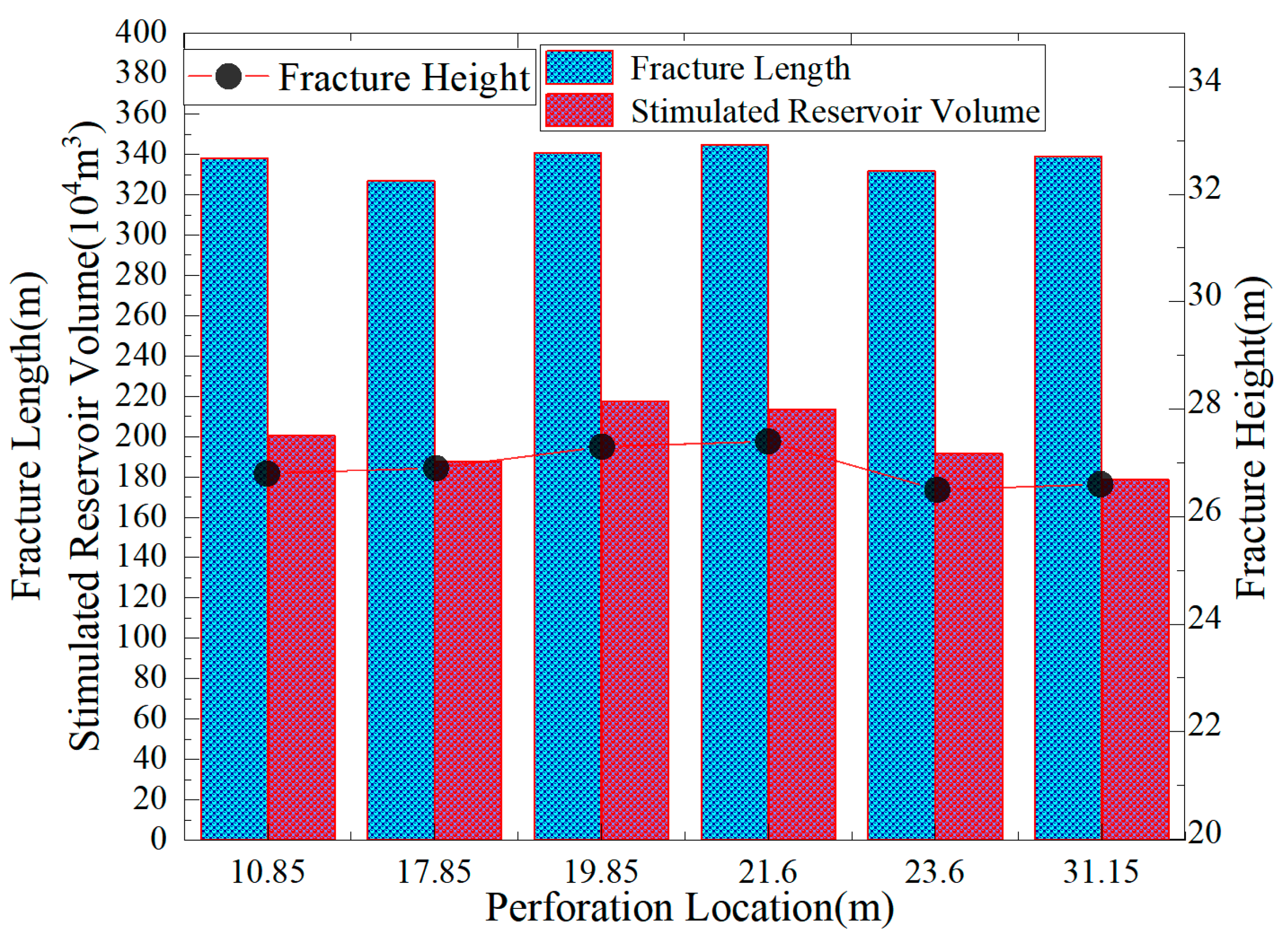
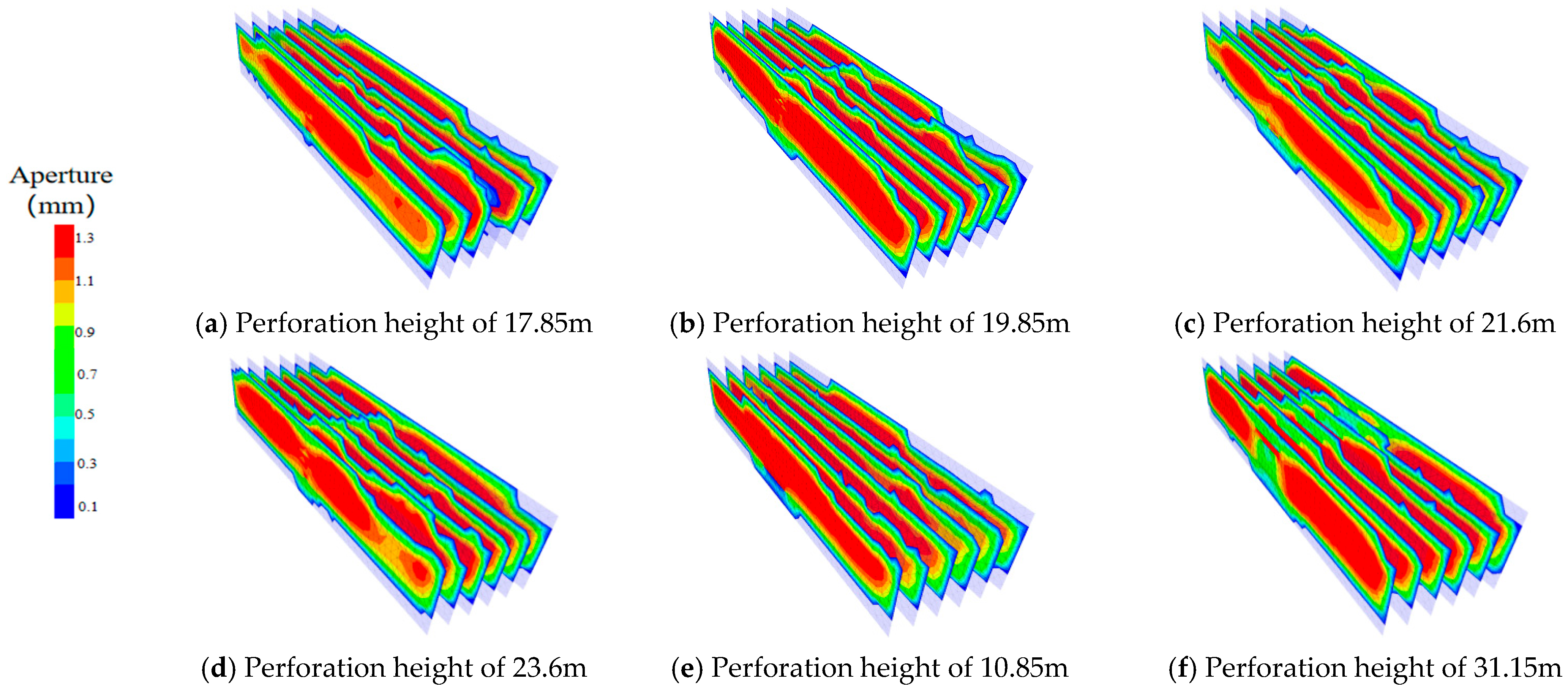
When the perforation location is in the range of 19.85–21.6 m (center of the main shale layer), the fracture height stabilizes at 26.8–27.4 m (Figure 30 and Figure 31). At this time, the perforation is located in the region with the most concentrated reservoir energy, and the fracture is easy to break through the upper interlayer into the upper shale. The vertical propagation is mainly in the upper part, with a relatively stable speed; when the perforation location is below the lower interlayer (10.85 m) or above the upper interlayer (31.15 m), the fracture height has no obvious advantage (26.5–26.6 m). Due to the deviation from the main reservoir, the energy is insufficient, the difficulty of breaking through the interlayer increases, and the vertical propagation speed is slow with a limited range.

The fracture length fluctuates slightly with the change in perforation location (332–345 m), but the stimulated reservoir volume (SRV) reaches the maximum value of 341–345 × 10⁴ m³ when the perforation location is 19.85–21.6 m (Figure 31 and Figure 32). At this time, the matching degree between the perforation location and the main shale is the highest, and the fracture can fully utilize the reservoir conditions for expansion, with high fracture network complexity; the SRV at both ends (10.85 m, 31.15 m) is low (332–338 × 10⁴ m³), due to the poor reservoir quality, the fracture expansion is limited, and the stimulation range is reduced.

4.4. Analysis of Dominant Factors Controlling Hydraulic Fracture Propagation in Interbedded Shale

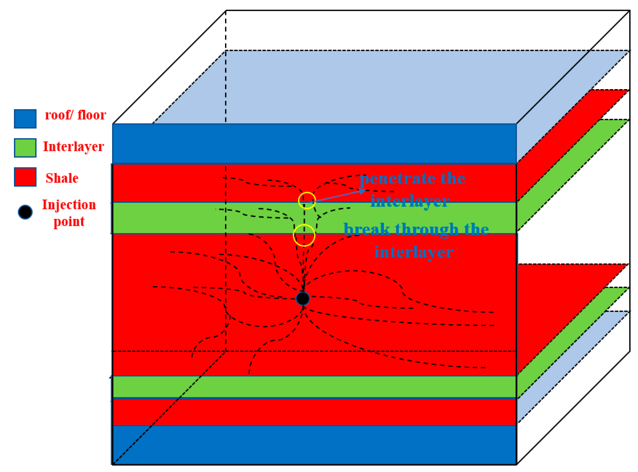
The propagation of hydraulic fractures in interbedded shale reservoirs is synergistically controlled by geological constraints and engineering operation parameters. Among numerous influencing factors, horizontal stress difference (Δσ), interlayer thickness (h), and pumping rate (Q) are the core dominant factors determining interlayer breakthrough behavior, as they directly regulate reservoir stress field distribution, energy transfer efficiency, and fracture propagation dynamics. In this section, grey relational analysis is introduced to systematically evaluate the degree of correlation between various influencing factors and the interlayer breakthrough response, based on the interlayer breakthrough statuses under different factors presented in

Table 4. Breakthrough of Interlayers under Different Factors.

Influencing Factor	Parameter Range	Upper Interlayer Breakthrough Status	Reason for Interlayer Breakthrough
Poisson’s Ratio	0.19~0.34	No Breakthrough	Weak influence; no significant effect
Young’s Modulus	25~50 GPa	No Breakthrough	Weak influence; no significant effect
Horizontal Stress Difference	≤16 MPa	Breakthrough	Low stress difference favors vertical propagation
	>16 MPa	No Breakthrough	High stress difference inhibits fracture height growth
Interlayer Thickness	≤2 m	Breakthrough	Thin interlayers are easily penetrated
	>2 m	No Breakthrough	Thick interlayers form an effective barrier
Pumping Rate	<16 m3/min	No Breakthrough	Insufficient energy; unable to break through
	16~18 m3/min	Breakthrough	Upper interlayer penetrated; partial entry into lower interlayer
	≥18 m3/min	Breakthrough	Further increase in rate has limited effect on lower interlayer penetration
Fluid Volume	<2200 m3	No Breakthrough	Insufficient fluid volume; limited fracture extension
	2200~2400 m3	Breakthrough	Upper interlayer can be penetrated
	≥2400 m3	Breakthrough	Increased volume assists partial entry into lower interlayer
Viscosity	<5 mPa·s	No Breakthrough	Weak proppant-carrying capacity; pressure easily dissipates in reservoir
	≥5 mPa·s	No Breakthrough	High viscosity promotes fracture height extension
Number of Clusters	5 clusters	Breakthrough	Concentrated energy; strong single-fracture penetration capability
	6–7 clusters	Breakthrough	Moderate energy dispersion; maximum SRV (Stimulated Reservoir Volume)
	≥8 clusters	No Breakthrough	Excessive energy dispersion; weakened breakthrough capability
Cluster Spacing	7 m	Breakthrough	Strong stress interference; edge clusters prone to breakthrough
	8~10 m	Partial Entry	Weakened stress interference; uniform extension
	≥11 m	No Breakthrough	Excessive spacing; diminished synergistic effect
Perforation Location	Center of main shale	Breakthrough	Most concentrated reservoir energy
	Off-center	No Breakthrough	Insufficient energy; increased breakthrough difficulty

The aim is to identify the key controlling factors governing interlayer breakthrough along with their critical conditions (Figure 33).

Grey relational analysis is applicable to uncertain systems with small samples and poor information. It determines the degree of correlation among factors by calculating the geometric similarity between each factor sequence and the reference sequence. The calculation steps are as follows:

(1) Determine the reference sequence and comparison sequences.

Take the breakthrough condition of the interlayer as the reference sequence X₀, and the parameter values of various influencing factors as the comparison sequences X_i. The breakthrough condition is quantified by assignment: breakthrough = 1, partial entry = 0.5, no breakthrough = 0.

(2) Perform dimensionless processing on the reference sequence and comparison sequences.

(3) Calculate the absolute difference between the interlayer breakthrough condition X₀ and different influencing factors X_i at corresponding time points, i.e.:

$${∆}_{0\mathrm{i}}\left({\mathrm{t}}_{\mathrm{j}}\right)={\mathrm{X}}_0\left({\mathrm{t}}_{\mathrm{j}}\right)-{\mathrm{X}}_{\mathrm{i}}\left({\mathrm{t}}_{\mathrm{j}}\right)$$

(23)

(4) Select the maximum value X0 and the minimum value Xi of the absolute differences between the interlayer breakthrough condition (${∆}_{\mathrm{m}\mathrm{a}\mathrm{x}}$) and the different influencing factors (${∆}_{\mathrm{m}\mathrm{i}\mathrm{n}}$).

Derive the correlation coefficient corresponding to the interlayer breakthrough condition and the different influencing factors, namely

$${\mathrm{L}}_{0\mathrm{i}}\left({\mathrm{t}}_{\mathrm{j}}\right)={\displaystyle \frac{{∆}_{\mathrm{m}\mathrm{i}\mathrm{n}}+{∆}_{\mathrm{m}\mathrm{a}\mathrm{x}}}{{∆}_{0\mathrm{i}}\left({\mathrm{t}}_{\mathrm{j}}\right)+{∆}_{\mathrm{m}\mathrm{a}\mathrm{x}}}}$$

(24)

where

$${∆}_{0\mathrm{j}}\left({\mathrm{t}}_{\mathrm{j}}\right)=\left|{\mathrm{X}}_{\mathrm{i}}-{\mathrm{X}}_0\right|$$

(25)

(5) Calculate the grey relational degree of each sequence.

$${\mathsf{\gamma }}_{0\mathrm{i}}={\displaystyle \frac{1}{\mathrm{n}}}{\sum }_{\mathrm{j}=1}^{\mathrm{n}}{\mathrm{L}}_{0\mathrm{i}}\left({\mathrm{t}}_{\mathrm{j}}\right)$$

(26)

The closer the relational degree ${\mathsf{\gamma }}_{0\mathrm{i}}$ is to 1, the more significant the influence of that factor on interlayer breakthrough.

Based on the data samples obtained from the numerical simulations in Section 4.3, a total of 11 factors were selected as comparison sequences, including geological parameters (Poisson’s ratio, Young’s modulus, horizontal stress difference, interlayer thickness, and interlayers in sub-layers 3 to 6), operational parameters (pumping rate, fluid volume, viscosity), and perforation parameters (number of clusters, cluster spacing, perforation location). Using the quantified interlayer breakthrough values as the reference sequence, the grey relational degree of each factor was calculated. The calculation results are presented in

Table 5. Grey Relational Degrees of Various Factors.

No.	Influencing Factor	Grey Relational Degree
1	Interlayer Thickness	0.908
2	Horizontal Stress Difference	0.892
3	Pumping Rate	0.874
4	Fluid Volume	0.851
5	Number of Clusters	0.612
6	Cluster Spacing	0.587
7	Viscosity	0.543
8	Perforation Location	0.501
9	Young’s Modulus	0.376
10	Poisson’s Ratio	0.258

.

The grey relational degree of interlayer thickness is the highest (0.908), indicating that it is the primary factor controlling interlayer breakthrough (Table 5). When the thickness is ≤2 m, the interlayer cannot effectively dissipate fracture energy and is easily penetrated; when the thickness exceeds 2 m, it forms an effective mechanical barrier. This is followed by the horizontal stress difference (0.892). Under low stress difference conditions (≤16 MPa), the horizontal confinement weakens, and the pressure within the fracture readily breaks through the upper interlayer; conversely, a high stress difference significantly inhibits vertical propagation. The pumping rate (0.874) and fluid volume (0.851) rank third and fourth, respectively, together constituting the energy supply system for fracturing.

The relational degrees of the other factors are all below 0.7, indicating a relatively weak influence on interlayer breakthrough. The number of clusters and cluster spacing indirectly affect breakthrough through stress interference, but their effects are secondary to parameters such as pumping rate and fluid volume. Viscosity influences fracture height extension but contributes only limitedly to breakthrough. Mechanical parameters such as Young’s modulus and Poisson’s ratio do not play a dominant role in the breakthrough process. Poisson’s ratio exhibits the lowest relational degree (0.258), confirming its insignificant effect on fracture propagation. In summary, whether a hydraulic fracture can break through the interlayer in interlayered shale is mainly governed by the synergistic control of four factors: interlayer thickness, horizontal stress difference, pumping rate, and fluid volume.

The reliable breakthrough of interlayers requires the simultaneous satisfaction of three critical conditions: horizontal stress difference Δσ ≤ 16 MPa, interlayer thickness h < 1 m, and pumping rate Q ≥ 16 m³/min. Under low stress difference (≤15 MPa), horizontal confinement is weakened, and the pressure inside the fracture readily induces tensile failure, penetrating the upper interlayer. When the stress difference exceeds 16 MPa, vertical propagation is hindered, and the breakthrough probability sharply decreases by 80% due to the high fracture toughness of the lower limestone interlayer. Thin interlayers (<1 m) cannot sufficiently dissipate fracture energy, resulting in a 65% probability of interface shear failure. When the thickness increases to ≥2 m, the breakthrough probability drops below 10%, accompanied by a 21% reduction in fracture height. When the pumping rate is below 16 m³/min, fluid loss leads to insufficient pressure accumulation. Once the threshold is reached, the pressure exceeds the initiation pressure to achieve breakthrough, and further increasing the pumping rate stabilizes the fracture height. The coupling effects among the three factors are significant: thin interlayers or low stress differences can lower the critical pumping rate, whereas thick interlayers (≥3 m) act as rigid constraints, making breakthrough difficult even at high pumping rates. This threshold system provides key theoretical support for optimizing fracturing parameters.

5. Conclusions

This study comprehensively investigates the propagation laws of complex fracture networks in interbedded shale through numerical simulation. The main conclusions are as follows:

(1)

Among geological parameters, an increase in stress difference leads to an increase in fracture length but a decrease in fracture height and SRV. A high stress difference is conducive to the lateral extension of fractures but inhibits the complexity of the fracture network; interlayer thickness is a key restrictive factor, and an increase in thickness significantly reduces fracture height, fracture length, and SRV, with the best stimulation effect when there are no interlayers.

(2)

For engineering parameters, pumping rate and fluid volume affect fracture propagation through a “threshold effect”: 16 m³/min for pumping rate and 2000 m³ for fluid volume are critical thresholds. Below the thresholds, the calcareous interlayer can be quickly broken through, and fracture height, fracture length, and SRV increase rapidly; beyond the thresholds, the propagation slows down. Viscosity has a significant influence: low viscosity (1 mPa·s) is conducive to vertical penetration of interlayers and formation of complex fracture networks, while high viscosity (30 mPa·s) extends fracture length but reduces SRV. The influence of fluid volume on stimulated volume is superior to that of pumping rate.

(3)

Regarding perforation parameters, the SRV is the largest when the number of clusters is 6–7, 5 clusters are conducive to fracture length extension, and an excessive number of clusters reduces the effect due to energy dispersion; the stress interference is minimal when the cluster spacing is 10 m, with optimal fracture length and SRV, and both too small or too large spacing are unfavorable; the best stimulation effect is achieved when the perforation location is 19.85–21.6 m (center of the main shale layer).

(4)

Thin interlayers or low stress differences can reduce the critical pumping rate, while thick interlayers (≥3 m) become the primary constraint, making breakthrough difficult even at high pumping rates. For interlayer breakthrough, the simultaneous satisfaction of Δσ ≤ 16 MPa, h < 1 m, and Q ≥ 16 m³/min is required.

This study systematically reveals, through numerical simulation, the propagation behavior of complex hydraulic fracture networks in shale reservoirs containing interlayers and clarifies the controlling effects of three categories of parameters—geological, engineering, and perforation. Specifically, high stress difference increases fracture length but suppresses fracture height; interlayer thickness acts as a key inhibiting factor. A pump rate of 16 m³/min and a fluid volume of 2000 m³ are identified as critical thresholds for penetrating calcareous interlayers. Low-viscosity fracturing fluid is more conducive to vertical breakthrough and the formation of complex fracture networks. The maximum stimulated reservoir volume (SRV) is achieved with 6–7 clusters, while a cluster spacing of 10 m minimizes stress interference. The study further quantifies the necessary conditions for interlayer breakthrough as a stress difference ≤ 16 MPa, an interlayer thickness <1 m, and a pump rate ≥ 16 m³/min. These findings provide a clear theoretical basis for fracturing optimization in such reservoirs. However, given the moderate simplifications of the model and the limitations of single-factor analysis under fixed operational parameters, it is recommended that future work incorporate reservoir heterogeneity to refine the extended model and explore dynamic intelligent fracturing technologies, thereby offering more comprehensive technical support for efficient stimulation and production enhancement in these reservoirs.

References

1. EIA. International Energy Outlook 2023; U.S. Energy Information Administration: Washington, DC, USA, 2023.
2. Palmer, I. Coalbed methane completions: A world view. Int. J. Coal Geol. 2010, 82, 184–195. [Google Scholar] [CrossRef] [Scilit]
3. Guo, X.; Hu, D.; Li, Y.; Liu, R.; Wang, Q. Geological Features and Reservoiring Mode of Shale Gas Reservoirs in Longmaxi Formation of the Jiaoshiba Area. Acta Geol. Sin. Engl. Ed. 2014, 88, 1811–1821. [Google Scholar] [CrossRef] [Scilit]
4. Zhou, Z.L.; Zhao, H.; Yang, D.S.; Qin, Y.L.; Zhuo, S.Q.; Cheng, W. Experimental study on the intersection of hydraulic fractures with thin interlayers. Eng. Fract. Mech. 2025, 327, 111465. [Google Scholar] [CrossRef] [Scilit]
5. Yang, Y.; Li, X.; Yang, X.; Li, X. Influence of reservoirs/interlayers thickness on hydraulic fracture propagation laws in low-permeability layered rocks. J. Pet. Sci. Eng. 2022, 219, 111081. [Google Scholar] [CrossRef] [Scilit]
6. Zhang, J.; Yu, Q.; Li, Y.; Pan, Z.; Liu, B. Hydraulic Fracture Vertical Propagation Mechanism in Interlayered Brittle Shale Formations: An Experimental Investigation. Rock Mech. Rock Eng. 2022, 56, 199–220. [Google Scholar] [CrossRef] [Scilit]
7. Zhang, J.; Xie, Z.; Pan, Y.; Tang, J.; Li, Y. Synchronous vertical propagation mechanism of multiple hydraulic fractures in shale oil formations interlayered with thin sandstone. J. Pet. Sci. Eng. 2023, 220, 111229. [Google Scholar] [CrossRef] [Scilit]
8. Suo, Y.; Su, X.; Wang, Z.; He, W.; Fu, X.; Feng, F.; Pan, Z.; Xie, K.; Wang, G. A study of inter-stratum propagation of hydraulic fracture of sandstone-shale interbedded shale oil. Eng. Fract. Mech. 2022, 275, 108858. [Google Scholar] [CrossRef] [Scilit]
9. Sheng, X.; Yang, L.; Wang, T.; Zhou, X.; Yu, H.; Zhang, Y.; Fu, X.; Mei, J.; Pei, Y. Hydraulic fracturing behavior of shale–sandstone interbedded structure under true triaxial stress conditions: A comprehensive experimental analysis. Fatigue Fract. Eng. Mater. Struct. 2024, 47, 1246–1261. [Google Scholar] [CrossRef] [Scilit]
10. Xue, Y.; Wang, L.C.; Liu, Y.; Ranjith, P.G.; Cao, Z.Z.; Shi, X.Y.; Gao, F.; Kong, H.L. Brittleness evaluation of gas-bearing coal based on statistical damage constitution model and energy evolution mechanism. J. Cent. South Univ. 2025, 32, 566–581. [Google Scholar] [CrossRef] [Scilit]
11. Yong, M.; Qingsheng, J.; Liaoyuan, Z.; Bintao, Z.; Xu, D. Research on Interlayer Interference and the Fracture Propagation Law of Shale Oil Reservoirs in the Dongying Sag. Pet. Drill. Tech. 2021, 49, 130–138. [Google Scholar]
12. Huang, L.; Deng, L.; Wu, A.; Du, F.; Wang, X.; Qian, L.; Lu, K. Investigating hydraulic fracture penetration in soft-hard interlayer coal measures with perforated completion. Eng. Fract. Mech. 2025, 327, 111467. [Google Scholar] [CrossRef] [Scilit]
13. Zhang, D.; Yi, L.; Yang, Z.; He, J.; Zhu, J.; Li, X.; Zhang, H. Numerical simulation study of proppant transport within fractures under the influence of interlayers and weak planes. Geomech. Energy Environ. 2025, 41, 100642. [Google Scholar] [CrossRef] [Scilit]
14. Lu, C.; Li, M.; Guo, J.C.; Tang, X.H.; Zhu, H.Y.; Yong-Hui, W.; Liang, H. Engineering geological characteristics and the hydraulic fracture propagation mechanism of the sand-shale interbedded formation in the Xu5 reservoir. J. Geophys. Eng. 2015, 12, 321–339. [Google Scholar] [CrossRef] [Scilit]
15. Lyu, J.; Hou, B.; Zhou, T. Fracture propagation behavior via multi-cluster fracturing in sandstone-shale interbedded reservoirs. Geoenergy Sci. Eng. 2024, 243, 213356. [Google Scholar] [CrossRef] [Scilit]
16. Sun, X.; Zhang, S.; Ma, X.; Zou, Y.; Lin, G. Experimental Investigation on Propagation Behavior of Hydraulic Fractures in Coal Seam during Refracturing. Geofluids 2019, 2019, 4278543. [Google Scholar] [CrossRef] [Scilit]
17. Liu, W.; Pan, Z.; Zhang, X.; Wei, Y.; Zhao, L.; Zhu, X.; Zhao, Y.; Guo, Q. Experimental Study of the Fracture Network Expansion Mechanism and Three-Dimensional Reconstruction Characteristic of High-Rank Coal in Guizhou Province, China. ACS Omega 2023, 8, 29803–29811. [Google Scholar] [CrossRef] [Scilit] [PubMed]
18. Feng, Z.Y. Height Detection and Analysis of Water Flowing Fractured Zone of Coal Face. Comput. Water Energy Environ. Eng. 2021, 10, 131–139. [Google Scholar] [CrossRef]
19. Wu, X.; Zhu, T.; Liu, Y.; Zhang, G.; Zheng, G.; Wang, F. Mechanism of Coal Seam Permeability Enhancement and Gas Outburst Prevention under Hydraulic Fracturing Technology. Geofluids 2022, 2022, 7151851. [Google Scholar] [CrossRef] [Scilit]
20. Fan, C.; Li, S.; Luo, M.; Yang, Z.; Lan, T. Numerical Simulation of Hydraulic Fracturing in Coal Seam for Enhancing Underground Gas Drainage. Int. J. Rock Mech. Min. Sci. 2019, 37, 166–193. [Google Scholar] [CrossRef] [Scilit]
21. Hamidi, F.; Mortazavi, A. A new three dimensional approach to numerically model hydraulic fracturing process. J. Pet. Sci. Eng. 2014, 124, 451–467. [Google Scholar] [CrossRef] [Scilit]
22. Zhi, C.; Bing, H.; Jihui, D. Competitive propagation simulation of multi-clustered fracturing in a cracked shale oil reservoir. Geomech. Geophys. Geo-Energy Geo-Resour. 2022, 8, 102. [Google Scholar]
23. Xue, Y.; Wu, W. Characterization of brittleness evolution of hot dry rock during cyclic thermal treatment. Acta Geotech. 2026. [Google Scholar] [CrossRef] [Scilit]
24. Itasca Consulting Group, Inc. 3DEC, Version 5.2; Itasca Consulting Group, Inc.: Minneapolis, MN, USA, 2016. Available online: https://www.itascacg.com/software/3dec (accessed on 16 February 2025).
25. Xiao, H.; Wang, H.; He, T.; Yuan, C.; Zhang, H. Propagation laws of complex fracture networks in cleated thin-layer coal rocks. Phys. Fluids 2025, 37, 083366. [Google Scholar] [CrossRef] [Scilit]
26. Bai, Y.; Hu, Y.; Liao, X.; Tan, J.; Zheng, Y.; Wang, W. Research on the influence of stress on the penetration behavior of hydraulic fracture: Perspective from failure type of beddings. Front. Earth Sci. 2023, 11, 1163295. [Google Scholar] [CrossRef] [Scilit]
27. Zheng, Y.; He, R.; Huang, L.; Bai, Y.; Wang, C.; Chen, W.; Wang, W. Exploring the effect of engineering parameters on the penetration of hydraulic fractures through bedding planes in different propagation regimes. Comput. Geotech. 2022, 146, 104736. [Google Scholar] [CrossRef] [Scilit]
28. Zheng, Y.; Liu, J.; Zhang, B. An investigation into the effects of weak interfaces on fracture height containment in hydraulic fracturing. Energies 2019, 12, 3245. [Google Scholar] [CrossRef] [Scilit]
29. Vera, F.; Shadravan, A. Stimulated Reservoir Volume 101: SRV in a Nutshell. In Proceedings of the International Petroleum Technology Conference, Doha, Qatar, 6–9 December 2015. [Google Scholar]
30. Xiao, H.; Zhang, H.; Wang, H.; Xie, X.; Wang, C.; Liu, J. Numerical Study on Hydraulic Fracture Propagation in Coalbed Methane Considering Coal Seam Cleats. Processes 2025, 13, 1036. [Google Scholar] [CrossRef] [Scilit]
31. Chang, X.; Qiu, G.; Li, J.; Guo, Y.; Hu, Z.; Yang, H.; Zhang, X.; Liu, Y. Study on the influence of vertical stress difference coefficient on fracture characteristics of shale under high stress. Energy Sci. Eng. 2024, 12, 3227–3242. [Google Scholar] [CrossRef] [Scilit]
Figure 1. Computational flowchart of the coupled BDEM and fluid flow model.
Processes 14 01341 g001
Figure 2. Schematic Diagram of Physical Model for Complex Fracture Network Propagation in Interbedded shale.
Processes 14 01341 g002
Figure 3. Schematic Diagram of Physical Model for Complex Fracture Network Propagation in Interbedded shale.
Processes 14 01341 g003
Figure 4. Fracture height and length of the Daye 1 platform.
Processes 14 01341 g004
Figure 5. 3D diagram of fracture propagation of the Daye 1H1-2.
Processes 14 01341 g005
Figure 6. Combination diagram of event points and fracture surfaces of the DY11H1-2. Top view of the combination of event points and fracture surfaces of the DY1 1H1-2 (Top). Side view of the combination of event points and fracture surfaces of the DY1 1H1-2 (Bottom).
Processes 14 01341 g006
Figure 7. Fracture height under different stress differences.
Processes 14 01341 g007
Figure 8. Relationship between stress difference and fracture length, fracture height, and stimulated reservoir volume.
Processes 14 01341 g008
Figure 9. 3D diagrams of fracture propagation under different stress differences.
Processes 14 01341 g009
Figure 10. Stress cloud maps under different stress differences.
Processes 14 01341 g010
Figure 11. Fracture height under different interlayer thicknesses.
Processes 14 01341 g011
Figure 12. Relationship between interlayer thickness and fracture length, fracture height, and stimulated reservoir volume.
Processes 14 01341 g012
Figure 13. 3D diagrams of fracture propagation under different interlayer thicknesses.
Processes 14 01341 g013
Figure 14. Stress cloud maps under different interlayer thicknesses.
Processes 14 01341 g014
Figure 15. Fracture height under different pumping rates.
Processes 14 01341 g015
Figure 16. Relationship between pumping rate and fracture length, fracture height.
Processes 14 01341 g016
Figure 17. 3D diagrams of fracture propagation under different pumping rates.
Processes 14 01341 g017
Figure 18. Fracture height under different fluid volumes.
Processes 14 01341 g018
Figure 19. Relationship between fluid volume and fracture length, fracture height, and stimulated reservoir volume.
Processes 14 01341 g019
Figure 20. 3D diagrams of fracture propagation under different fluid volumes.
Processes 14 01341 g020
Figure 21. Fracture height under different viscosities.
Processes 14 01341 g021
Figure 22. Relationship between viscosity and fracture length, fracture height, and stimulated reservoir volume.
Processes 14 01341 g022
Figure 23. 3D diagrams of fracture propagation under different viscosities.
Processes 14 01341 g023
Figure 24. Fracture height under different numbers of clusters.
Processes 14 01341 g024
Figure 25. Relationship between number of clusters and fracture length, fracture height, and stimulated reservoir volume.
Processes 14 01341 g025
Figure 26. 3D diagrams of fracture propagation under different numbers of clusters.
Processes 14 01341 g026
Figure 27. Fracture height under different cluster spacings.
Processes 14 01341 g027
Figure 28. Relationship between cluster spacing and fracture length, fracture height, and stimulated reservoir volume.
Processes 14 01341 g028
Figure 29. 3D diagrams of fracture propagation under different cluster spacings.
Processes 14 01341 g029
Figure 30. Fracture height under different perforation locations.
Processes 14 01341 g030
Figure 31. Relationship between perforation location and fracture length, fracture height, and stimulated reservoir volume.
Processes 14 01341 g031
Figure 32. 3D diagrams of fracture propagation under different perforation locations.
Processes 14 01341 g032
Figure 33. Schematic diagram of hydraulic fracture breakthrough in interbedded reservoirs.
Processes 14 01341 g033