Article

Short-Term Wind Power Non-Crossing Quantile Forecasting Based on Two-Stage Multi-Similarity Segment Matching

by
Dengxin Ai
1,
Li Zhang
1,
Junbang Lv
2,
Song Liu
3,
Zhigang Huang
3 and
Lei Yan
2,*
1
Electric Power Research Institute of State Grid Tianjin Electric Power Company, Tianjin 300384, China
2
College of Electrical Engineering, Yuquan Campus, Zhejiang University, Hangzhou 310058, China
3
State Grid Tianjin Electric Power Company, Tianjin 300384, China
*
Author to whom correspondence should be addressed.
Processes 2026, 14(8), 1310; https://doi.org/10.3390/pr14081310
Submission received: 24 March 2026 / Revised: 16 April 2026 / Accepted: 17 April 2026 / Published: 20 April 2026
(This article belongs to the Special Issue Applications of Smart Microgrids in Renewable Energy Development)

Abstract

Accurate wind power forecasting is essential for the stability of modern power systems. However, current probabilistic forecasting frameworks often encounter a fundamental conflict between the computational efficiency required for high-dimensional meteorological pattern matching and the physical consistency of the resulting probability distributions. Existing methods frequently fail to maintain the logical monotonicity of quantiles or overlook the fine-grained temporal correlations in massive historical datasets. To address these critical gaps, this research develops a comprehensive framework that synergizes a hierarchical similarity filtering mechanism with a structurally constrained non-crossing quantile regression model. First, the target sample is partitioned into several weather segments, and a new two-stage high-similarity weather pattern matching method is developed to screen multiple sets of historical samples that are highly similar to the target weather pattern. Second, a deep learning model for probabilistic wind power quantile forecasting is proposed, which incorporates historical data augmentation. The model utilizes an attention mechanism to extract the correlation between the target and historical segments, while an improved non-crossing quantile regression model is adopted to ensure the validity of the output quantiles. Finally, the effectiveness of the proposed method is validated through case studies using real-world data from an actual wind farm.

1. Introduction

In recent years, to address the issues of environmental degradation and increasing energy demand resulting from the massive consumption of fossil fuels, the installed capacity of renewable energy, particularly wind energy, has been increasing annually worldwide [1,2]. However, due to the instability of weather conditions, the inherent randomness of wind energy poses significant challenges to the power balance and the secure, stable operation of power systems [3,4]. As a key technology to tackle such challenges, wind power forecasting (WPF) has received considerable attention in recent decades. It helps to mitigate the operational risks arising from the fluctuations of high-penetration wind power and is of great significance for ensuring the safe and reliable operation of the power system [5,6,7].
Much of the previous research on wind power forecasting has primarily focused on deterministic point forecasting. This approach, however, is subject to unavoidable errors caused by the instability of meteorological factors and fails to provide detailed information on uncertainty. To quantitatively characterize the uncertainty of wind power, increasing attention has been directed towards probabilistic wind power forecasting [8].
Probabilistic wind power forecasting is mainly categorized into parametric and non- parametric methods. The former assumes that the wind power forecasting error follows a known probability distribution model, and consequently, the complete probability distribution can be determined by predicting the parameters of this known distribution. Commonly used distribution functions for parametric methods include the Beta, Gaussian, and Logit-normal distributions [9,10]. Ref. [11] employed a Gaussian Mixture Model to model the wind power forecasting error and introduced a Variational Bayesian method to optimize the model, thereby outputting probabilistic forecasts of wind power. Ref. [12] utilized the Lorenz disturbance distribution to describe the fluctuation range and trend of wind speed to achieve high-quality wind speed interval prediction. However, the true probability distribution of wind power is unknown. When the assumed probability density function deviates significantly from the actual distribution of the forecast power, the forecasting performance can hardly be guaranteed.
In contrast, non- parametric methods do not make a priori assumptions. Instead, they utilize techniques such as kernel density estimation (KDE) [13], the Cornish-Fisher expansion [14], and quantile regression (QR) [15] to perform a non-linear mapping, thereby calculating the quantiles of the predicted power’s probability density function (PDF) or cumulative distribution function (CDF). Among these, the QR method is targeted at predicting quantiles, describing the probability distribution of future power using a set of quantiles. Traditional QR methods typically require building separate prediction models for different quantiles, which can lead to the erroneous phenomenon of quantile crossing, where a higher quantile is smaller than a lower one [16]. To address this, Ref. [17] constructed a non-crossing sparse group quantile regression deep neural network model, which introduces a penalty term for non-crossing constraints into the loss function to enforce the monotonicity of different quantile outputs, thus effectively mitigating the quantile crossing phenomenon. Other studies have also integrated the constraints for non-crossing quantiles into the design of the prediction module [18,19,20,21]. For example, Ref. [20] constructed a non-crossing quantile neural network that represents higher-order quantiles as the sum of a lower-order quantile and a non-negative increment; whereas Ref. [21] proposed an improved non-crossing quantile regression (INCQR) strategy that generates strictly monotonically increasing quantile predictions through an exponential sum mapping. In addition to imposing constraints on the model structure or loss function, Ref. [22] adopted a unified quadratic spline quantile function to characterize the entire conditional probability distribution, overcoming the limitation of traditional quantile methods that can only predict fixed quantiles and providing more comprehensive predictive information.
Recent studies have shown that, considering the diversity of weather patterns, adopting strategies based on classification and pattern selection can effectively improve the accuracy of WPF. For instance, Ref. [23] proposed a clustering method based on fluctuation trend decomposition, which segments wind speed series into fluctuation periods using wavelet transform and then groups these periods using an improved Fuzzy C-Means (IFCM) algorithm. Ref. [24], on the other hand, constructed a dual-dimensional clustering framework that utilizes both meteorological and historical power features to build the sample set, achieving automatic sample grouping via the K-means algorithm. Historical sample matching based on sequence similarity is also one of the primary methods for pattern selection. Ref. [25] used multi-feature similarity indices to match the target forecast segment with multiple similar historical days for wind power forecasting modeling and prediction, further improving accuracy by refining the distance calculation formula. Previous studies have predominantly used Euclidean distance or correlation coefficients to calculate sample similarity [26,27]. Other research has proposed multi-parameter similarity matching for wind processes and selecting an appropriate forecasting model for each process, which further improved the accuracy of deterministic point forecasting for wind power under different weather scenarios [28]. Although these similarity-matching methods based on historical samples offer high accuracy, they may suffer from excessive computational load when dealing with large volumes of high-resolution historical data, leading to a reduction in the overall speed of the method.
Currently, traditional methods for wind power forecasting mainly include physical models and statistical models. Physical model-based methods primarily predict the future power output of wind turbines based on the wind turbine power curve, topographical data, and Numerical Weather Prediction (NWP) data such as wind speed, wind direction, temperature, and air pressure for the forecast period [29]. Statistical methods rely on historical operational data to build predictive models, and their forecasting performance is directly linked to the quantity and quality of the historical data. Typical methods include Autoregressive Moving Average (ARMA) [30] and Autoregressive Integrated Moving Average (ARIMA) [31]. However, both physical and statistical models are limited by their inability to capture the complex non-linear relationships between meteorology and power, resulting in poor predictive performance.
In recent years, artificial intelligence technologies such as machine learning and deep learning have attracted widespread attention due to their excellent non-linear fitting and parameter learning capabilities, and have been widely applied in the field of wind power forecasting [32,33]. Ref. [32] proposed a deep mixture density network to directly predict the wind speed probability density function, fusing a Convolutional Neural Network (CNN) and a Gated Recurrent Unit (GRU) to learn temporal features, and demonstrated significant superiority over various advanced methods in terms of sharpness, accuracy, and reliability. Ref. [33] proposed two hybrid deep learning models, ABiLSTM and Transformer-MLP, which utilize CNNs to capture short-term patterns in wind power, and achieved results superior to baseline models such as CNN, BiLSTM, and Transformer in long-term and short-term wind power forecasting, respectively.
Despite the progress in non-parametric probabilistic forecasting, two significant scientific challenges remain unresolved. First, similarity-based pattern selection in extensive meteorological databases faces a bottleneck where simple distance metrics cannot capture local evolutionary details, while complex metrics incur prohibitive computational costs. Second, deep learning-based quantile regression models generally lack an inherent mathematical mechanism to prevent quantile crossing, leading to logically inconsistent forecasts during volatile weather conditions. This research addresses these limitations by establishing a theoretical bridge between multi-scale pattern recognition and monotonically constrained distribution modeling. The main highlights and innovations of this paper are as follows:
  • First, a hierarchical two-stage multi-similarity segment matching (TSMSSM) algorithm is developed. The architecture decouples global trend screening from local pattern alignment, thereby narrowing the search space. This approach facilitates both computational efficiency and high-precision pattern recognition within large-scale databases, overcoming the computational bottlenecks of traditional dynamic alignment methods.
  • Second, a non-crossing quantile regression (NCQR) model is proposed that integrates structural monotonicity constraints. Unlike conventional incremental optimizations, this model utilizes an exponential summation mapping and a parametric activation function to theoretically guarantee the non-decreasing property of the quantile function. This mathematical design eliminates quantile crossing at the structural level while enhancing the capture of conditional distribution features through historical data augmentation.
  • Third, a synergistic enhancement between the matching and forecasting modules is achieved. The highly relevant historical context dynamically extracted by TSMSSM empowers the exponential sum mapping of the NCQR to generate sharper prediction intervals without compromising coverage reliability, effectively advancing beyond the capabilities of isolated forecasting models.
Section 2 introduces the relevant concepts and overall methodological framework for day-ahead wind power probabilistic forecasting. Section 3 elaborates on the proposed two-stage multi-similarity hybrid matching method and the coupled short-term non-crossing quantile prediction model. Section 4 discusses the effectiveness and superiority of the proposed model through case studies. Finally, Section 5 provides the research conclusions and future outlook.

2. Related Concepts and Overall Methodological Framework

2.1. Related Concepts and Data Description

This study primarily addresses a day-ahead short-term wind power forecasting problem, which uses the previous day’s Numerical Weather Prediction (NWP) data to predict the expected value and probability distribution of power for a single wind farm. The forecast time scale is 24 h with a time resolution of 15 min. All data used in this study were sourced from actual data of multiple wind power stations in a regional power grid of a certain province in China, including NWP data, actual measured wind power data, and station capacity. Detailed information about this data is shown in Table 1, and all data have been cleaned for missing and anomalous values.
The NWP vector for the t -th 15 min interval of a day is denoted as N W P t , including wind speed and direction data for four different floor heights, as well as temperature, relative humidity and air pressure data. Consequently, a full day’s NWP sample can be represented as S a m p l e   =   { N W P 1 , , N W P i , N W P 96 } . For historical samples, their NWP data, power forecast data, and actual measured power data are all known; whereas for the target sample to be forecasted, only the NWP data and power forecast data are known.
Based on the partitioning of samples, this paper further introduces weather segments W s e g and power measurement segments P s e g as the basic units of analysis, defined as W s e g   =   { N W P i , N W P i   +   1 , , N W P i   +   τ     1 } , P s e g = { P P , i , , P P , i   +   τ     1 } . Here, τ is the length parameter of the time window.

2.2. Overall Framework for Short-Term Wind Power Non-Crossing Quantile Forecasting Based on TSMSSM

The overall framework of the proposed short-term wind power non-crossing quantile prediction based on two-stage multi-similarity hybrid matching is shown in Figure 1. It is mainly divided into two core parts: a two-stage multi-similarity hybrid matching method and a short-term wind power non-crossing quantile prediction model.
In the multi-similarity hybrid matching part, this paper proposes a two-stage multi-similarity matching algorithm that uses multiple weather segment similarity indices. The method first partitions the historical samples and the target day’s sample into a historical weather segment set W S e g H I S T and a target day weather segment set W S e g F C S T according to different strategies. For each target weather segment, Stage 1 utilizes two computationally efficient indices to rapidly screen historical samples, selecting those within the top ranking percentage to form a candidate pool. Stage 2 then evaluates these candidates comprehensively using a composite index integrating two advanced metrics. Ultimately, the top N s historical segments and their corresponding power profiles are extracted as the matched results.
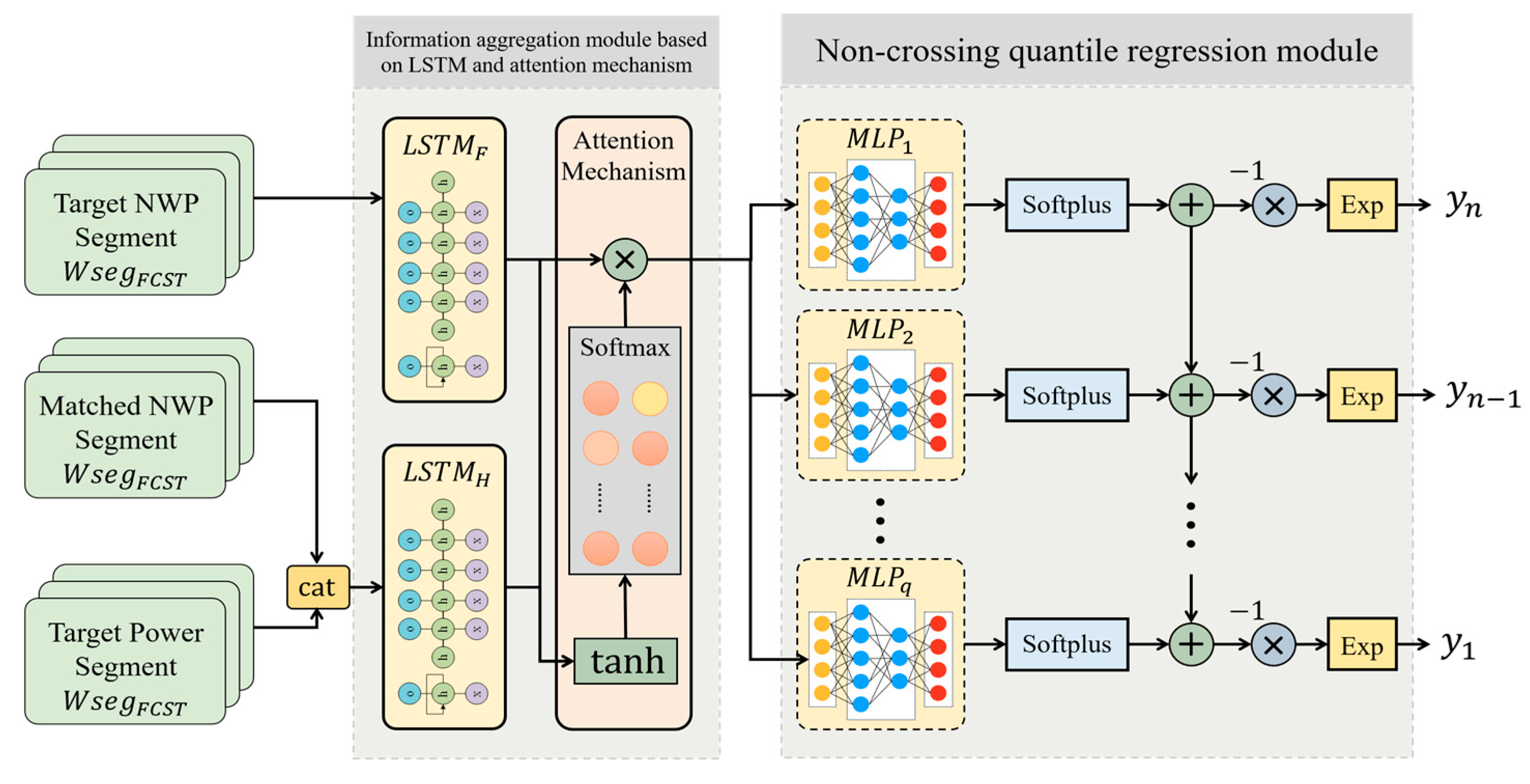
The second component is a deep learning-based, improved non-crossing quantile regression model. For each target segment, the model takes as input the segment itself and its matched historical counterparts (including both weather and power data). An inter-segment attention mechanism, combined with Long Short-Term Memory (LSTM), is leveraged to extract critical features and relationships among these segments, encoding the information into a high-dimensional vector. This vector is then processed by a non-crossing quantile prediction module, which serves as a decoder. This module maps the vector to the final quantile forecasts while inherently guaranteeing their monotonicity.
The above-mentioned multi-similarity hybrid matching and non-crossing quantile prediction process is repeated for each segment in the target day until the probabilistic wind power forecast for the entire target day is completed.

3. Methodology

3.1. Two-Stage Multi-Similarity Segment Matching

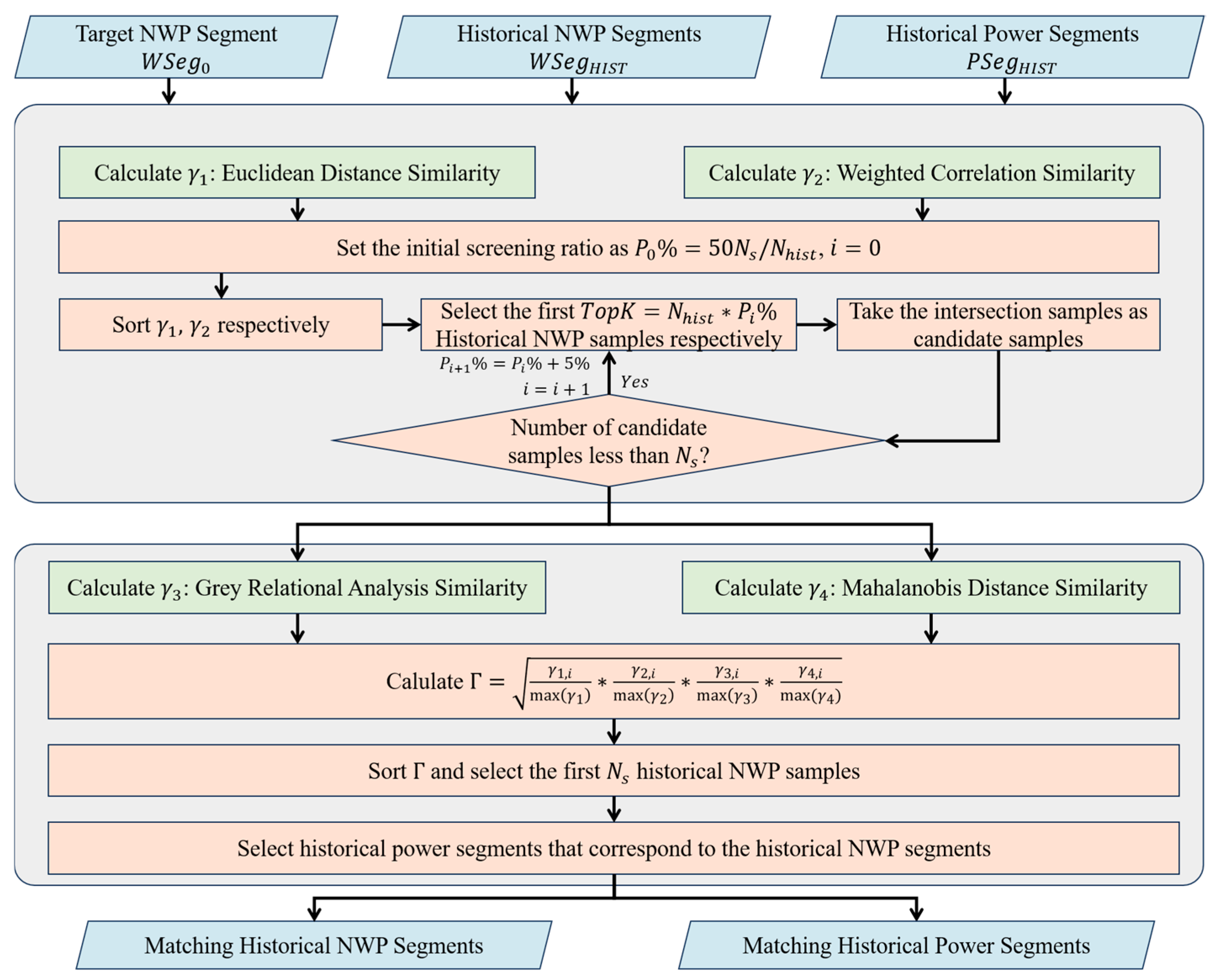
This subsection elaborates on the technical details of the proposed two-stage multi-similarity segment matching (TSMSSM) method; its overall framework is shown in Figure 2. It first analyzes weather segment similarity and defines the relevant indices, and then presents in detail the two-stage matching method based on fast screening and precise matching, providing a detailed workflow.
Many studies have used two indices, distance and the correlation coefficient, to measure the similarity between two weather segments. Specifically, distance is utilized to represent the difference between the two segments, while the correlation coefficient is used to determine whether the two segments have similar variation trends [34,35]. Other studies have further proposed more complex indices and achieved favorable results. Based on this, this paper proposes four similarity indices and divides the matching process into two stages: a rapid screening stage based on simple indices such as distance and correlation coefficient, and a precise matching stage based on complex indices.

3.1.1. Rapid Screening Stage

  • Distance Similarity Index  γ 1 . This index is used for a preliminary and rapid assessment of the distance between the wind speed segments of two weather segments. Its calculation is shown in Equation (1). First, the mutually perpendicular U-V wind speed components are calculated from the wind speed and wind direction. Then, γ 1 is defined as the multiplicative inverse of the Euclidean distance of the wind speed components.
    γ 1 , i = 1 j = 1 8 k = 1 τ V 0 , j , k V i , j , k 2 + ε
    where V is the U-V wind speed sub-features (m/s) in the NWP data, with a total of eight wind speed components at four different floor heights; and ε is a very small positive value to prevent the denominator from being zero. In this study, it is set to 0.0001 (10−4). The subscripts of the variable V , from left to right, denote the segment index, the sub-feature index, and the temporal index within the segment, respectively. For instance, V 0 , j , k   represents the k -th data point of the j -th sub-feature sequence in the target sequence, while V i , j , k represents the k -th data point of the j-th sub-feature sequence within the i -th historical segment. A larger value of γ 1 , i indicates that the magnitudes of the wind speed segment V 0 and V i are closer. Since wind speed is the determining factor of wind power generation, a larger γ 1 , i also implies that the power curves corresponding to V 0 and V i should exhibit higher similarity.
  • Trend Similarity Index  γ 2 . γ 2 determines the similarity between the target and historical weather segments by assessing the similarity of their wind speed trends. To accurately capture the dynamic trend similarity between time series, we propose a weighted correlation coefficient method based on difference sequences. The calculation is detailed in Equations (2)–(5):
    V i , j , k   = V i , j , k + 1 V i , j , k ,     k = 1 , 2 , , τ 1
    w i , j , k = 1 2 V 0 , j , k + V i , j , k
    D W C V 0 , j , V i , j = k = 1 τ 1 w i , j , k V 0 , j , k V 0 , j ¯ V i , j , k V i , j ¯ k = 1 τ 1 w i , j , k V 0 , j , k V 0 , j ¯ 2 k = 1 τ 1 w i , j , k V i , j , k V i , j ¯ 2
    γ 2 , i = 1 8 j = 1 8 D W C V 0 , j , V i , j
    where V i , j , k represents the difference sequence of the meteorological segment, and w i , j , k is a weighting coefficient associated with the magnitude of the difference sequence, designed to emphasize the importance of fluctuation characteristics. The terms V 0 , j ¯ and V i , j ¯ denote the mean values of the difference sequences V 0 , j and V 0 , j , respectively. The value of D W C V 0 , j , V i , j ranges from −1 to 1, where a value closer to 1 indicates consistent upward trends, while a value closer to -1 signifies consistent downward trends. From a more intuitive perspective, a γ 2 , i value closer to 1 signifies that the local trends of V 0 and V i are more consistent, meaning that the increments or decrements at any given moment are more aligned. Furthermore, the introduction of the weight coefficient w i , j , k increases the weighting of fluctuations with larger magnitudes in the calculation of γ 2 , i , thereby enhancing the sensitivity of this metric to local fluctuations.
  • Rapid screening based on similarity Indices ranking. Historical samples are ranked independently by distance γ 1 and trend γ 2 similarities. We select the intersection of the top P % from both rankings to form the candidate pool. The initial threshold is set to P 0 %   =   50 N s / N h i s t . To ensure algorithmic robustness, if this intersection yields fewer than N s candidates, P % is iteratively expanded by a step size of P %   =   5 % until the pool size reaches at least N s .

3.1.2. Precise Matching Stage

Following the rapid screening stage, we obtain a candidate historical segment pool that is significantly reduced in size yet exhibits high similarity to the target segment in terms of macroscopic distance and variation trends. However, the accuracy of wind power prediction is highly dependent on the precise capture of dynamic details in wind speed, such as the periodicity of fluctuations and the complex coupling relationships between different meteorological elements. Simple distance and trend indices are insufficient to fully characterize these underlying features.
Therefore, in the precise matching stage, this paper introduces a more sophisticated similarity measure. This method is designed to re-rank the candidate segments from the perspectives of multi-scale morphology and intrinsic structure and correlation, with the aim of identifying the historical samples that are most similar to the target segment in their dynamic evolutionary patterns.
  • Grey Relational Analysis Similarity Index  γ 3 . This study employs Grey Relational Analysis (GRA) [36] to assess the closeness of the interconnection between different sequences by calculating the similarity of their U-V components of wind speed at various heights. The grey relational coefficient between the target segment and the i -th historical segment for the j -th sub-feature is calculated as shown in Equation (6):
    ξ V 0 , j , V i , j = 1 τ k = 1 τ min j   min k V 0 , j , k V i , j , k + ρ   max j   max k V 0 , j , k V i , j , k V 0 , j , k V i , j , k + ρ   max j   max k V 0 , j , k V i , j , k
    where ρ is the distinguishing coefficient taken as 0.5. Based on the GRA correlation coefficient, the calculation of the similarity index γ 3 is shown in Equation (7):
    γ 3 , i   =   j   =   1 8 ξ V 0 , j , V i , j 8
    Leveraging Grey Relational Analysis (GRA), γ 3 , i serves as an effective measure for the temporal correlation of wind speed sequences across various heights, addressing the insufficiency of the numerical distance γ 2 , i in capturing non-linear interdependencies.
  • Mahalanobis Distance Similarity index  γ 4 . Since wind power is typically a result of the collective influence of wind speeds across multiple heights, which are inherently interdependent, the Mahalanobis distance utilizes a historical covariance matrix to partially decouple these cross-height correlations. Consequently, this enables similarity evaluation within a transformed, independent state space. This paper proposes a fourth similarity index, γ 4 based on the Mahalanobis distance. First, the Mahalanobis distance for the wind speed features at each time step is calculated using Equation (8):
    D M V 0 , k , V i , k = V 0 , k V i , k T Σ 1 V 0 , k V i , k  
    where is a high-dimensional vector comprising all wind speed sub-features for the i -th segment at the k -th time step. Σ is the covariance matrix between these sub-features, which is computed from the entire historical dataset as Equation (9):
    Σ =   1 n     1 V   1 μ T T V   1 μ T
    where V R n   ×   d (with d   =   8 ) represents the historical U-V wind speed data matrix, μ R d   ×   1 is the mean vector of V , 1 R n   ×   1 is an all-ones column vector. The matrix V   1 μ T effectively centers the historical data by subtracting the respective feature means. The global covariance matrix Σ is pre-computed offline, utilizing only the training dataset to strictly prevent data leakage. After obtaining the corresponding Mahalanobis distances, the similarity between the target and the i -th historical segment, denoted as γ 4 , i is computed via Equation (10):
    γ 4 , i   =   1 1   +   1 τ k   =   1 τ D M V 0 , k , V i , k
  • Combinational Similarity Index  Γ . Based on the aforementioned distance and trend similarity indices, we establish a combined similarity index, Γ , for the precise matching. A higher value of Γ indicates greater similarity between the historical and target segments, as defined in Equation (11):
    Γ i   = γ 1 , i max γ 1   ·   γ 2 , i max γ 2   ·   γ 3 , i max γ 3   ·   γ 4 , i max ( γ 4 )
    A key design consideration is the integration of metrics with different scales and physical significance. To mitigate the resulting difficulty in weight assignment, a two-step strategy is adopted: first, each similarity metric is normalized using the max function; second, they are combined using the geometric mean instead of the arithmetic mean.
Finally, the top N s historical weather prediction samples ranked by Γ , along with their corresponding ground-truth power measurements, constitute the final output of the TSMSSM. In this study, N s is taken as 10.

3.1.3. Summary of TSMSSM Algorithm

In summary, the TSMSSM algorithm optimizes the trade-off between computational tractability and matching precision via a hierarchical filtering mechanism. Stage 1 utilizes efficient metrics ( γ 1 , γ 2 ) to rapidly prune the high-dimensional search space based on macroscopic weather trends. Subsequently, Stage 2 applies advanced metrics ( γ 3 , γ 4 ) to perform microscopic feature alignment on the reduced candidate pool. Notably, γ 4 leverages the Mahalanobis distance to decouple highly correlated wind variables into an orthogonal state space, ensuring unbiased similarity evaluation. This dual-stage design provides a robust and highly efficient data foundation for the forecasting module.

3.2. Non-Crossing Quantile Prediction Deep Learning Model

This subsection details the proposed non-crossing quantile prediction neural network deep learning model and the loss function used for its training. On one hand, the use of limited historical data is of great significance for providing more accurate prediction interval information for quantile prediction models, a fact confirmed by many studies [37,38]. On the other hand, high-reliability quantile prediction requires the monotonicity of the model’s output quantiles, whereas previous deep learning models that predict quantiles independently have difficulty handling the quantile crossing problem well due to the difficulty of adding non-crossing constraints.
Based on the above motivations, this paper proposes a non-crossing quantile prediction neural network that fuses information from similar historical samples. As shown in Figure 3, the model is mainly composed of two main modules: an Information Aggregation module based on LSTM and an attention mechanism, and a Non-Crossing Quantile Regression (NCQR) module.

3.2.1. Information Aggregation Module Based on LSTM and Attention Mechanism

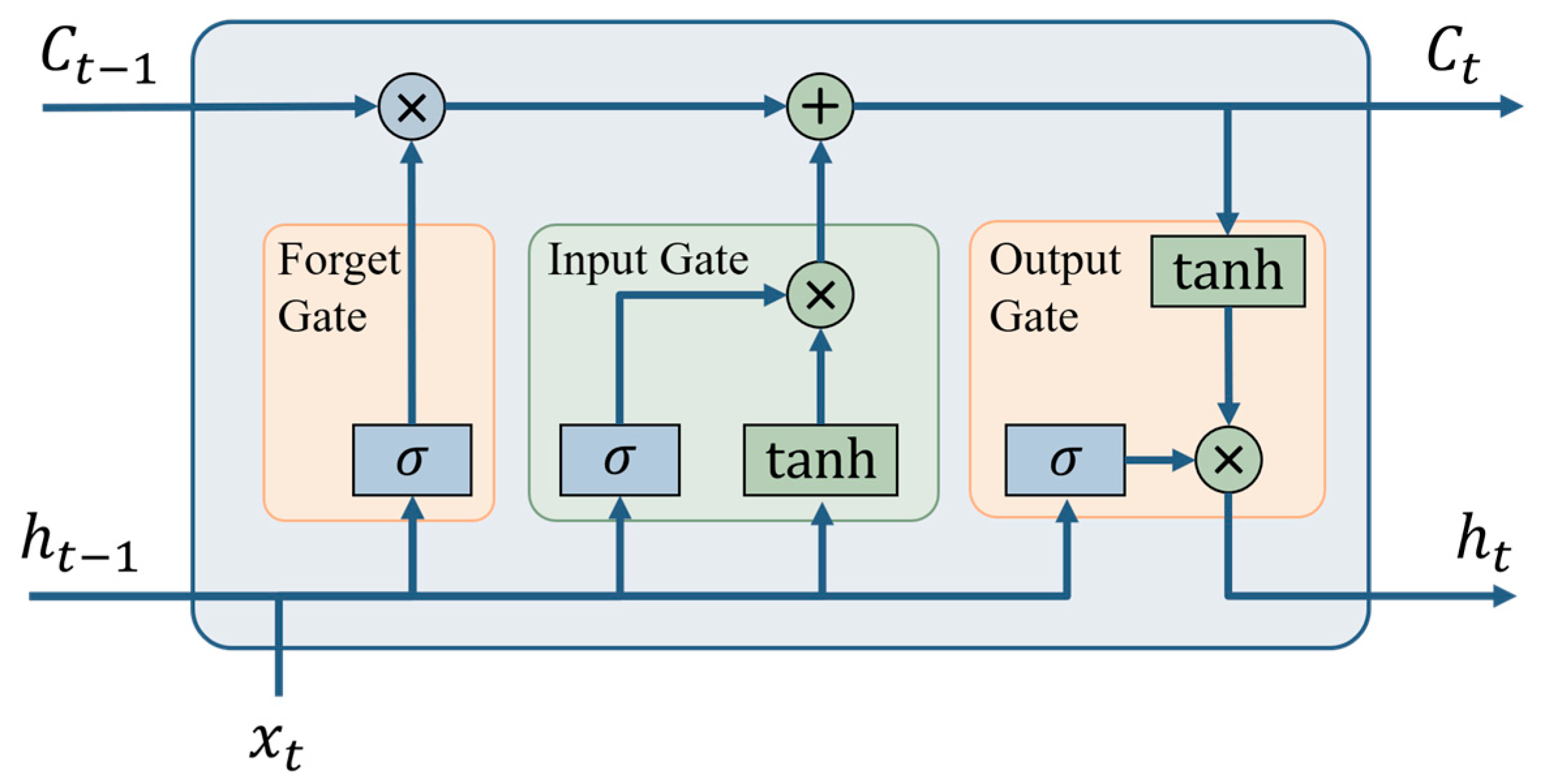
  • Long Short-Term Memory (LSTM) Network. The LSTM introduces gating structures into the Recurrent Neural Network (RNN) foundation, achieving better performance in processing time series. An LSTM unit is mainly composed of a memory cell state and its three gating structures, with its specific internal structure shown in Figure 4. The principle of the LSTM unit can be summarized as: after inputting the memory cell state information c t     1 and hidden layer state h t     1 from the previous moment into the current unit, and combining them with the current input sequence x t , the three gating structures control the retention and discard of information to calculate the current memory cell state information c t and hidden layer state h t . Its calculation process is as shown in Equation (12):
    f t = s i g m o i d W f · h t 1 , x t + b f i t = s i g m o i d W i · h t 1 , x t + b i o t = s i g m o i d W o · h t 1 , x t + b o c ~ t = tanh W c · h t 1 , x t + b c c t = f t c t 1 + i t c ~ t h t = o t tanh c t
    where W f ,   W i , W o ,   W c are trainable weight matrices, and b f ,   b i , b o ,   b c are learnable biases; h t 1 is the hidden state from the previous moment, x t is the input sequence at the current moment, and denotes the Hadamard product operation.
Based on the above process, the final output hidden state of the LSTM unit contains information from all previous inputs.
This study uses an LSTM to process the input historical segment set X i   =   x i , k   =   x N W P , i , k , x P M , i , k k   =   1 τ and the target NWP segment X 0   =   x 0 , k k   =   1 τ , and obtains the corresponding high-dimensional hidden state sequences H i   =   h i , k k   =   1 τ , H 0   =   h 0 , k k   =   1 τ .
h i , k = L S T M H x i , k , h i , k 1 h 0 , k = L S T M F x 0 , k , h 0 , k 1  
where x N W P , i , k represents the feature vector composed of various NWP values at time index k of the i -th historical NWP segment, x P M , i , k represents the power measurement value at time index k of the i -th historical power measurement segment, and x 0 , k represents the feature vector at time index k of the target NWP segment. H i represents the high-dimensional vector obtained after the i -th historical segment is processed by the LSTM unit, and H 0 is the high-dimensional vector transformed from the target segment.
2.
Information Aggregation based on Attention Mechanism. The attention mechanism is a technique that allows the model to focus on important information and fully learn and absorb it. In time series prediction tasks, it can adaptively assign different weights to different historical samples, thereby more effectively extracting information most relevant to the current prediction target. In this module, the input to the attention mechanism is the set of high-dimensional vectors H = { H 0 , H 1 , , H N s } extracted by the LSTM. Its goal is to calculate the attention weights of the historical samples { H 1 , , H N s } relative to the target sample H 0 and generate a context vector that fuses all relevant information. The attention score between samples is calculated by Equation (14):
e i , k = v a T tanh W a · h 0 , k , h i , k + b a
where v a T ,   W a and b a are all learnable weight matrices and vectors. Next, the Softmax function is used to convert the attention scores into normalized attention weights a i , k , whose magnitude reflects the importance of the i-th historical sample for predicting the target sample at moment k.
a i , k = exp e i , k i = 1 N s exp e i , k
The vector representations of the historical samples are weighted and summed according to their corresponding attention weights to obtain the final high-dimensional representation:
c k   =   i   =   1 N s a i , k h i , k

3.2.2. Non-Crossing Quantile Regression Module

Theoretically, predicted quantiles should increase as the quantile level increases. However, traditional deep learning models usually use a method of independently predicting different quantile outputs, which leads to a lack of necessary constraints on the output quantiles, and the problem of quantile crossing occurs when predicted values are low or quantile levels are compact. Inspired by other research to ensure the monotonicity of the quantile function, this paper proposes a non-crossing quantile regression module.
To mathematically eliminate such feasibility and optimality failures, the proposed NCQR module abandons penalty-based approaches in favor of a hard structural constraint. As governed by Equation (17), the module utilizes an exponential sum mapping. If activation stringently forces all intermediate quantile elements m k into the strictly positive domain ( m k   =   m k , j j   =   1 n ,   m k , j   >   0 ), the negative summation within the exponential function guarantees that the outputs are bounded within (0,1) and are strictly monotonically increasing. This design maps the unconstrained output space of the dense layers , directly into a strictly feasible monotonic probability space, ensuring that the predicted quantiles remain logically valid under any cases.
y ^ k α i = exp j = 1 n i + 1 m k , j
To ensure the strict monotonicity of the quantile predictions, this paper makes certain improvements to the activation function that generates the quantile elements m k based on Ref. [19], replacing the original ReLU with a Parametric Softplus (PSoftplus). Moreover, compared to the “dying ReLU” problem caused by the ReLU function when the input is non-positive, the PSoftplus ensures that its gradient is always greater than zero over its domain, which is beneficial for the stability and effectiveness of model training. The proposed PSoftplus is defined as Equation (18):
P S o f t p l u s β x   =   1 β ln 1   +   e β x ,         β   >   0
where β is a configurable parameter used to control the degree of smoothness. When β   =   1 , PSoftplus is the standard Softplus, and as β , it approaches ReLU. In this work, this value is set to 2.
A brief proof demonstrating that this module guarantees the strict monotonicity of quantile predictions is provided as follows:
Proposition 1 .
Let  A = α i i = 1 n  be a set of quantile levels such that  0 <   α 1 < α 2 < < α n < 1 . For any two indices  i  and  j  satisfying  1 i   < j   n , the predicted quantiles  y ^ k α i  and  y ^ k α j  at the moment generated by the proposed NCQR module satisfies  y ^ k α i <   y ^ k α j .
Proof. 
According to the definition of the NCQR module, the predicted quantiles for the levels α i and α j are formulated as:
y ^ k α i   =   exp l   =   1 n     i   +   1 m k , l y ^ k α j   =   exp l   =   1 n     j   +   1 m k , l
where m k , l denotes the quantile elements output by the PSoftplus activation function. Since the range of PSoftplus is strictly positive, we have m k , l > 0 for all l 1 , , n .
Given that i   < j , it follows that n   i   + 1 > n   j   + 1 . Consequently, we can write:
l   =   1 n     i   +   1 m k , l   =   l   =   1 n     j   +   1 m k , l l   =   n     j   +   2 n     i   +   1 m k , l   <   l   =   1 n     j   +   1 m k , l
Owing to the fact that the exponential function exp x is a strictly monotonically increasing function over its entire domain, applying it to both sides of the inequality yields:
exp l   =   1 n     i   +   1 m k , l   <   exp l   =   1 n     j   +   1 m k , l
which implies:
y ^ k α i   <   y ^ k α j
Thus, the proposed method theoretically ensures the strict monotonicity of the quantile predictions, effectively preventing the quantile crossing problem.
For the prediction problem with n quantile levels, a quantile element prediction module based on a Multi-Layer Perceptron (MLP) is proposed, which independently predicts the quantile elements m k , j for different quantile levels through n MLPs. A single MLP is a basic feedforward neural network, composed of several hidden layers and an output layer. Each layer consists of several neurons, with neurons between adjacent layers being fully connected and transformed by a non-linear activation function. The output of the l -th hidden layer can be expressed as Equation (23):
h k , j l   =   φ 1 , j W 1 , j · c k   +   b 1 , j             l   =   1 φ l , j W l , j · h k , j l     1   +   b l , j       2     l     L M L P
The final output of the k-th MLP is the quantile element corresponding to the respective quantile level:
m k , j   =   φ o , j W o , j · h k , j L M L P   +   b L M L P
where W ,   b ,   φ are the weights, biases and activation functions for each hidden layer, respectively, and L M L P is the number of hidden layers in the MLP. □

3.2.3. Model Training Based on H-Pinball Loss Function

This paper uses the improved Huber-norm pinball (H-pinball) loss function as the loss function for training the model, and its formula is shown in Equations (25) and (26):
ρ y , y ^ q , η   =   y     y ^ q η 2 ,         y     y ^ q     η y     y ^ q 2 2 η ,         y     y ^ q   <   η
L H y , y ^ q = q ρ y , y ^ q , η ,                                 y y ^ q     0 1 q ρ y , y ^ q , η ,         y y ^ q < 0
where η   >   0 is a threshold. Based on this, the complete loss function can be expressed as Equation (27):
L H   =   1 L k q L H y k , y ^ k q
Compared to the general pinball loss function, the H-pinball loss function is differentiable at zero. Additionally, to improve training efficiency, the Adam optimizer and batch training techniques are used to train the proposed model.

3.2.4. Summary of the NCQR Model

The proposed forecasting model achieves a seamless integration of adaptive feature extraction and physical constraint enforcement. The information aggregation module leverages an attention mechanism to dynamically learn complex temporal correlations between the target and matched historical segments. Furthermore, the NCQR module’s mathematical design―transforming strictly positive elements into final forecasts―provides an inherent guarantee of monotonicity across all quantile levels. This structural innovation effectively resolves the quantile crossing problem, ensuring that the predicted probability distributions are both data-driven and logically consistent.

4. Case Study

This case study is structured as follows. The first section details the experimental setup, which includes the dataset used for model training and testing, the performance evaluation metrics, and the baseline models for comparison. The second section presents the training and testing results of the proposed wind power quantile forecasting model. Through a systematic comparison with the baseline methods, the effectiveness and superiority of the proposed method are validated. The third section provides an in-depth discussion and analysis of the forecasting results.

4.1. Experiments Description

4.1.1. Data Description

As shown in Table 1, this case study utilizes historical datasets from four distinct real-world wind farms, spanning two years with a 15-min resolution. The NWP data from all wind farms were standardized using the maximum value normalization method. Additionally, the power generation data were standardized based on their respective installed capacities. Any power generation data exceeding the installed capacity was limited within the capacity range to ensure that all standardized power generation data fall within the interval of [0, 1].

4.1.2. Dataset Construction

To construct the dataset for training, the raw meteorological forecast data and wind power measurements were processed into the required format. First, the dataset was partitioned as detailed in Table 2: the training set contains 511 days of data (69.90%), while the validation and testing sets contain 109 days (14.91%) and 111 days (15.18%), respectively.
At the segmentation level, distinct strategies were employed for target and historical segments. For all datasets, a non-overlapping window sampling method with a window length of τ was used to generate the target segments to be forecasted. The number of target segments per day is given by Equation (28):
N f o r e   =   96 τ
where τ is the sampling window length. To ensure complete coverage of all time points within a day, τ must be a divisor of 96, i.e., τ { 2 , 3 , 4 , 6 , 8 , 12 , 16 , 24 , 32 , 48 } . Based on preliminary experiments and analysis.
The segmentation of historical segments was applied exclusively to the training and validation sets. For each daily sample in these sets, a sliding window sampling method with a step size of s and a window length of τ was applied. The number of historical segments derived from one day of data is calculated as Equation (29):
N h i s t   =   96     τ s   +   1
Similar to τ , the step size s should also be a divisor of 96 and satisfy s   <   τ to ensure all time points are considered. In this study, s was set to 4, corresponding to one hour in the actual data. This sampling strategy not only effectively increases the quantity of historical segments but also mitigates the issue of failing to match similar segments due to temporal shifts. The resulting numbers of target and historical segments are summarized in Table 3. Furthermore, during the matching stage in training and validation, target segments within the historical data are excluded to prevent them from being matched with themselves.

4.1.3. Hyperparameters and Training Strategy of Proposed Method

The experimental framework is implemented using Python 3.10 and PyTorch 2.8. The data pipeline is executed as follows: raw power and NWP data are preprocessed using NumPy 2.2 and Pandas 2.3, following the cleaning and normalization procedures described in Section 4.1.1. The TSMSSM algorithm (Section 3.1) functions as a dynamic data-loading layer, providing augmented input for the information aggregation module (Section 3.2) of the proposed model. All deep learning models are trained on an NVIDIA RTX A6000 GPU workstation. After segment-level inference, the final daily wind power quantiles are extracted by concatenating predicted intervals and calculating metrics against ground-truth measurements.
Regarding the similarity calculation, parameters were handled via two strategies to balance adaptability and reproducibility. Standard algorithmic constants, such as the distinguishing coefficient ρ in Grey Relational Analysis, were fixed at 0.5 in accordance with classical literature to avoid overfitting. Structural hyper-parameters, including the target matching number ( N s   =   10 ), the time window length ( τ   =   12 ), and the step size ( s   =   4 ) were optimally tuned via grid search on the validation set. To ensure a fair comparison, all matching methods, including the baseline approaches, utilize the identical built-in sorting function provided by NumPy 2.2.
The training hyperparameters adopted in the deep learning model are detailed in Table 4. The LSTM layer has a hidden dimension of 32 and consists of 1 layer. The attention mechanism module also has 1 layer with a hidden dimension of 64. Each MLP has 64 neurons in its hidden layer and uses the GELU activation function. All the hyperparameters involved above have been independently optimized using the grid search method. The case studies in this research involve comparisons with baseline models. To ensure the fairness of the comparative experiments, all baseline models underwent hyperparameter tuning via grid search under the condition that their total number of trainable parameters differs by no more than 50% from that of the proposed model. This ensures that each model achieves its optimal performance state, thereby excluding any performance gains resulting from the parameter scale. To eliminate stochastic bias, the parameters of all deep learning models are initialized using PyTorch’s built-in default methods. Furthermore, the Adam optimizer is uniformly employed, along with identical early stopping and learning rate warmup strategies.

4.2. Evaluation Metrics

4.2.1. Deterministic Forecasting

To effectively evaluate the performance of the proposed wind power forecasting model, metrics such as Mean Absolute Error (MAE) and Root Mean Square Error (RMSE) were employed. For the quantile forecasts produced by our model, the deterministic metrics are primarily applied to the median forecast (i.e., the 0.5 quantile). MAE and RMSE measure the magnitude of the deterministic forecasting error, while the coefficient of determination (R2) assesses the goodness-of-fit between the 0.5-quantile forecast and the actual power curve. An R2 value closer to 1 indicates higher accuracy for the deterministic forecast.
M A E = 1 N i = 1 N y i y ^ i 0.5
R M S E = 1 N i = 1 N y i y ^ i 0.5 2
R 2 = 1 i = 1 N   y i     y ^ i 0.5 2 i = 1 N y i y ¯ 2
where N is the number of samples, y i is the observed power at time i , and y ¯ is the mean of the observed power y i .

4.2.2. Quantile Forecasting

For quantile forecasting, Pinball loss, Mean Absolute Reliability Error (MRAE), Normalized Average Prediction Sharpness (NAPS), and Continuous Ranked Probability Score (CRPS) are introduced as evaluation metrics, as shown in Equations (33)–(39). Pinball loss is a fundamental metric for quantile regression models, which evaluates the accuracy of specific quantile forecasts by assigning asymmetric penalties to overestimation and underestimation behaviors. MRAE measures the reliability of quantile forecasts by calculating the absolute difference between the empirical coverage and the nominal quantile level. In probabilistic forecasting, MRAE reflects the calibration of the predictive distribution. A well-calibrated model ensures that the predicted probabilities align closely with the observed frequencies. High reliability is a critical prerequisite for power system operation; without accurate calibration, the quantitative uncertainty information could mislead downstream risk management and reserve allocation. NAPS measures the concentration of quantile forecasts by calculating the average interval width of the predictive distribution. A lower NAPS means lower uncertainty in quantile forecasting and reduced flexible resource requirements, thereby improving the economic efficiency of the power system.
L P y i , y ^ i q = q · y i y ^ i q ,                                 y i y ^ i q     0 1 q · y i y ^ i q ,             y i   y ^ i q < 0
p i n b a l l = 1 N i q L P y i , y ^ i q
M R A E = 1 n i = 1 n q i q ^ i
q ^ i = 1 N i = 1 N η ^ i q i
η ^ i q i = 1 ,       y i     y ^ i q i 0 ,       y i > y ^ i q i
N A P S = 1 N A i = 1 N α A y ^ i 1 α y ^ i α 1 2 α
where q i is the nominal proportion, and is its corresponding empirical coverage; α is the lower bound of the prediction interval, and 1 α is the upper bound; A denotes the number of intervals in the set of evaluated quantile intervals.
In probabilistic forecasting, MRAE reflects the calibration of the predictive distribution. A well-calibrated model ensures that the predicted probabilities align closely with the observed frequencies. High reliability is a critical prerequisite for power system operation; without accurate calibration, the quantitative uncertainty information could mislead downstream risk management and reserve allocation.
However, there is a significant conflict between MRAE and NAPS, which cannot fully reflect the comprehensive performance of the model’s probabilistic forecasting. Therefore, we adopt CRPS as the fourth metric. CRPS comprehensively evaluates the overall deviation between the predicted probability distribution and the actual observations, effectively balancing reliability and sharpness. In practical operation, a lower CRPS means the predictive distribution can more accurately characterize wind power uncertainty, thereby providing higher-quality boundary conditions for the stochastic economic dispatch of the power system.
C R P S = 1 N i = 1 N F y i z I y i < z 2 d z
where F y i z represents the cumulative distribution function (CDF) of the predicted probability outcome; I y i   <   z is an indicator function that takes the value of 1 only when the condition within the parentheses is satisfied, and 0 otherwise. Moreover, since the work of this paper predicts quantile results, directly calculating the CRPS is extremely difficult; Therefore, in this paper, we actually adopt the CDF approximation algorithm based on the Python properscoring library.

4.3. Evaluation of TSMSSM

4.3.1. Introduction of Benchmark Methods

To evaluate the TSMSSM algorithm, two benchmark methods are introduced for comparison:
  • Benchmark M1: A K-means-based approach that utilizes the multiplicative inverse of the Euclidean distance between sequences as the similarity metric. It clusters target and historical segments into the same group to facilitate rapid screening of similar patterns.
  • Benchmark M2: A Dynamic Time Warping (DTW) method [39,40], where the similarity index is derived from the multiplicative inverse of the DTW distance between wind processes.
To assess and compare the computational efficiency across multiple scales, experiments were conducted, including single-sample matching, as well as full matching for all samples in the validation and testing sets. All methods utilize the training set samples specified in Table 3 as the historical database, with the number of output matched samples ( N s ) set to 10 for all cases.

4.3.2. Evaluation of Computational Efficiency

As shown in Table 5, the proposed TSMSSM algorithm demonstrates a significant advantage in computational efficiency across all time scales. Specifically, for a single segment matching, the computation time of TSMSSM is only 0.0618 s. This represents a speedup of approximately 52 times compared to Benchmark 1 (3.2238 s) and an improvement of over two orders of magnitude compared to the computationally intensive Benchmark 2 (17.4764 s).
This disparity in efficiency becomes even more pronounced when processing large-scale datasets. In the full-sample matching experiments for the validation and testing sets, TSMSSM efficiently completes all computations within 44s. In contrast, Benchmark 1 requires over 2100 s (approx. 35 min) for the same data volume, while Benchmark 2 exceeds 3600 s due to the high computational overhead inherent in the DTW algorithm. These experimental results validate that the two-stage matching strategy of the TSMSSM method effectively reduces the frequency of reliance on complex metric calculations, fundamentally ensuring high computational efficiency and real-time responsiveness under large-scale data conditions.
The dramatic reduction in computation time achieved by TSMSSM, as demonstrated in the large-scale test set matching, provides a critical advantage for real-world energy management systems. While traditional benchmarks like DTW or K-means become computationally prohibitive as the database grows, the proposed dual-stage strategy maintains sub-second responsiveness. This evidence suggests that the framework is not merely a numerical improvement but a viable solution for the transition toward high-penetration renewable grids, where thousands of wind farms must be processed simultaneously under tight market-clearing windows.
To further substantiate the efficiency advantages observed in Table 5, we conducted a theoretical analysis of computational complexity and scalability. It should be noted that identifying the top N s segments most similar to the target necessitates sorting the candidate segments. The time complexity of this operation is generally O N log N , an unavoidable computational overhead shared by all matching algorithms based on similarity ranking. The speed advantage of the proposed algorithm is primarily concentrated in the similarity computation stage: the Stage 1 rapid screening relies on Euclidean distance and difference sequence calculations, operating at a linear complexity of O N · τ that is proportional to the sample size N and the time window length τ . Crucially, the computationally intensive metrics in Stage 2 are strictly executed on a drastically reduced candidate pool of size M   N s     M     N , reducing the time complexity of this phase to O M · τ . In contrast, the DTW typically exhibits a quadratic time complexity of O N · τ 2 when calculating sequence alignments, and the K-means clustering approach operates at O I · K · N · τ , where K and I denote the number of clusters and iterations, respectively. This theoretical comparison fundamentally explains the significant sub-second computational advantage of the proposed TSMSSM algorithm over M1 and M2, as empirically demonstrated in Table 5.

4.4. Evaluation of NCQR Module

4.4.1. Introduction of Benchmark Methods

To verify the effectiveness of the NCQR component, an ablation study was conducted by comparing the following four models: M1: The proposed comprehensive deep learning model that retains the NCQR module. Benchmark models M2/M3/M4: The NCQR module is substituted with the non-crossing quantile modules employed in Ref. [19], Ref. [20], and Ref. [21], respectively, with the remainder of the deep learning architecture kept intact. These alternative non-crossing quantile techniques represent the state-of-the-art in wind power quantile forecasting over recent years. To guarantee an equitable comparison, all evaluated models (M1–M4) are implemented within an identical experimental environment mentioned in Section 4.1.3.

4.4.2. Evaluation of Quantile Prediction

Table 6 presents the quantile forecasting error evaluation metrics of models M1–M4 on the test sets of four wind farms, where the best and second-best results are highlighted in bold and underlined, respectively.
In terms of the Pinball loss, M1 is slightly ahead of the second-best model M4, which can be considered as basically a tie, and is significantly ahead of M2 and M3, with the maximum improvement reaching 10.7%. For the MRAE metric, M1 shows a relatively obvious improvement over the second-best model M4 on most wind farms, reaching 12.9% to 34.2%; it only slightly lags behind M4 by about 7.7% on XWZ. This indicates that the proposed M1 has broader applicability.
A special case is the NAPS metric, on which M3 achieved the best performance, and it significantly outperformed the second-best model on all wind farms, with a lead ranging from 9.6% to 10.9%. Meanwhile, the M1 model achieved the second-best performance on three wind farms (NG, SJT, and XWZ), and only slightly lagged behind M4 by 0.5% on MZ. On the CRPS metric, similar to the Pinball metric, M1 and M4 are basically tied, with M1 leading by a slight advantage. Overall, the quantitative comparison among the four wind farms (MZ, NG, SJT, and XWZ) clearly shows that the proposed NCQR model (M1) exhibits a significant performance advantage.
It is worth acknowledging that M3 consistently achieves the lowest NAPS across all stations, indicating that its ReLU-based architecture is highly effective at generating narrow prediction intervals. However, this extreme sharpness appears to come at the expense of probabilistic reliability. As reflected by its significantly higher MRAE and CRPS, the rigid zero-bounding of the ReLU activation in M3 can force adjacent quantiles to converge, effectively shrinking the interval width but risking under-coverage. This highlights a classic trade-off in probabilistic forecasting: while M3 prioritizes interval sharpness, the proposed NCQR module (M1) strikes a more scientifically balanced trade-off, ensuring logical strict monotonicity and superior overall distribution quality (CRPS) without sacrificing too much sharpness.

4.5. Evaluation of the Proposed WPF Method Based on TSMSSM and Non-Crossing Quantile Forecast Deep Learning Model

In this section, the proposed wind power forecasting (WPF) method―which integrates TSMSSM with NCQR deep learning model―is compared against six distinct benchmark models to validate its superiority in both deterministic and probabilistic forecasting. First, the benchmark methods utilized for comparison are introduced. Second, the results of the model training and prediction are illustrated. Third, the forecasting performance of each method is analyzed and compared based on deterministic and uncertainty-based evaluation metrics. Finally, ablation studies are presented to verify the individual contribution and effectiveness of each module within the proposed framework in enhancing predictive accuracy.

4.5.1. Introduction of Benchmark Methods

This subsection introduces the benchmark wind power forecasting methods utilized for the comparative experiments, which encompass six typical deep learning models: MLP, LSTM [41], CNN-LSTM [22], CNN-Transformer (CNN-XMFR) [33], INCQR [21], and EDNQR [19]. Specifically, MLP and LSTM serve as foundational time-series benchmarks to illustrate the fundamental improvements of the proposed architecture. CNN-LSTM and CNN-Transformer (CNN-XMFR) are selected as they represent the recent state-of-the-art in spatiotemporal feature extraction and deterministic wind power forecasting. Furthermore, INCQR and EDNQR are chosen because they are the most recent and highly relevant advanced models specifically designed to address the non-crossing quantile regression problem. Comparing against them establishes a rigorous and direct evaluation of the probabilistic forecasting superiority of our proposed NCQR module. All benchmark models were implemented in the same experimental environment as mentioned in Section 4.1.3.

4.5.2. Evaluation of Deterministic Prediction

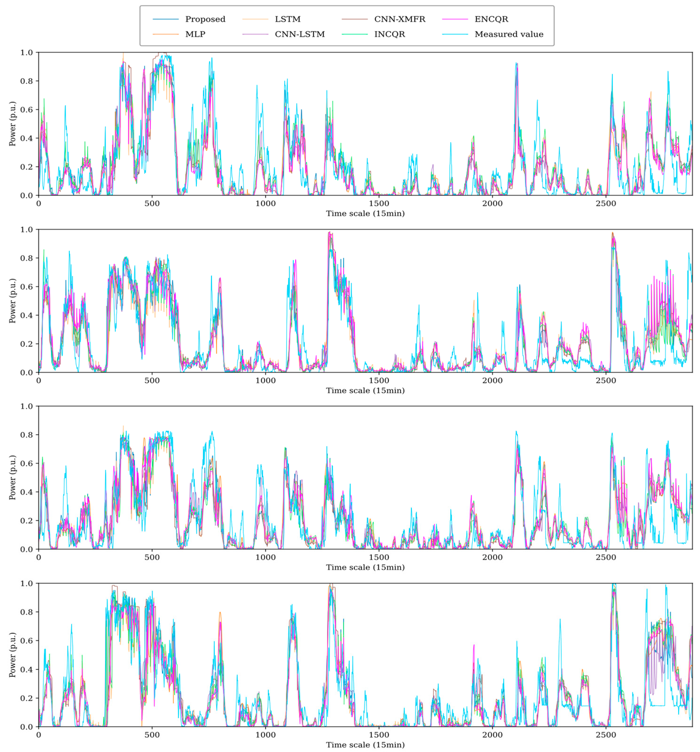
This subsection first compares the deterministic forecasting performance of the proposed method against several benchmark models. For the aforementioned quantile prediction models, the predicted values at the 0.5 quantile are selected as the deterministic results. The comparison of deterministic error metrics for the six models (including the proposed one) is summarized in Table 7, where the best and second-best results are highlighted in bold and underlined, respectively. Based on the MAE and RMSE metrics across different wind farm test sets, the proposed model outperforms all benchmark models in the vast majority of scenarios and metrics. Notably, it achieves the best performance in terms of MAE and R2 across all scenarios. Specifically, for wind farm MZ, the MAE and RMSE of the proposed method are reduced by 0.81% and 0.80% compared to the second-best model, and represent an improvement of 2.30% and 2.37% over the worst-performing model. For wind farm NG, the MAE is 0.32% lower than that of the second-best model, while the RMSE differs from the best model by only 0.14%. Regarding wind farms SJT and XWZ, the proposed method reduces the MAE by 1.04% and 0.68%, and the RMSE by 0.85% and 1.21%, respectively, compared to the second-best results. In terms of R2, the proposed model shows an improvement ranging from 0.33% to 3.45% across all sites compared to recent advanced models, CNN-LSTM, INCQR, and EDNQR. Detailed comparisons of the deterministic forecasting results for each wind farm are illustrated in Figure 5.

4.5.3. Evaluation of Quantile Prediction

As demonstrated by the comparison of the multi-dimensional evaluation metrics in Table 8, the proposed model exhibits superior probabilistic forecasting performance on the datasets from four real-world wind farms. It holds a significant advantage, particularly in the comprehensive metrics measuring overall distribution quality.
In terms of pinball loss, the proposed model achieves the optimal values across all four stations: MZ, NG, SJT, and XWZ. Compared to the second-best performing models, it realizes performance improvements of 3.12%, 0.82%, 1.05%, and 0.25% at each respective station. Similarly, regarding the CRPS metric, which evaluates the overall accuracy of probabilistic forecasting, the proposed model delivers the best performance at the MZ, NG, and SJT stations, outperforming the second-best models by 0.62%, 0.33%, and 1.11%, respectively. Furthermore, it ties for first place with the best counterpart model at the XWZ station. These results fully demonstrate the advanced capability of the proposed model in quantile forecasting.
For the NAPS metric, which measures the sharpness of prediction intervals, the proposed model attains the best results at the SJT and XWZ stations with values of 0.3214 and 0.3372, indicating significant enhancements of 3.40% and 1.32% over the second-best models, respectively. At the NG station, the proposed model yields an NAPS of 0.3195, lagging behind the optimal EDNQR model by only a marginal gap of approximately 0.57%. Although the CNN-Transformer achieves the best NAPS at the MZ station, it exhibits suboptimal performance in terms of MRAE. Conversely, regarding the MRAE metric, which reflects the reliability of prediction intervals, the LSTM model obtains the minimum values at the MZ, NG, and XWZ stations but fails to balance this with its NAPS performance. The detailed numerical comparisons presented above strongly corroborate the effectiveness of the proposed model, validating that it achieves superior performance in striking a balance between the sharpness and reliability of prediction intervals.
While the numerical improvements in metrics such as MAE (up to 1.04% reduction) and Pinball loss (up to 3.12% reduction) over state-of-the-art benchmarks (e.g., CNN-Transformer, EDNQR) may appear numerically modest, their practical significance in large-scale power system operations is profound. In the highly mature field of short-term wind power forecasting, pushing the boundaries beyond highly optimized deep learning architectures is inherently challenging. Furthermore, these accuracy gains are achieved simultaneously with a sub-second computational speedup and a strict structural guarantee against quantile crossing. Thus, the proposed framework delivers a systemic operational breakthrough rather than merely an incremental numerical tweak.
Furthermore, a deeper critical analysis of the reliability (MRAE) and calibration of the predictive distributions reveals a fundamental trade-off inherent in quantile forecasting. As shown in Table 8, while the proposed model achieves competitive MRAE scores, it does not universally yield the absolute lowest values; for instance, the baseline LSTM model achieves slightly better reliability at the MZ (0.0132 vs. 0.0231), NG (0.0206 vs. 0.0257), and XWZ (0.0100 vs. 0.0124) stations. However, evaluating calibration solely through MRAE can be misleading. The LSTM achieves these high-reliability scores at the severe cost of sharpness, outputting consistently wider prediction intervals. The model artificially inflates coverage by sacrificing precision, which reduces the economic efficiency of power dispatch.
In contrast, the proposed NCQR model imposes a strict structural constraint (exponential summation mapping) to prevent quantile crossing. This structural regularization forces the cumulative distribution function (CDF) to remain logically consistent, preventing unphysical probability distortions. Consequently, the proposed model achieves a much more balanced calibration, reflected by its superior comprehensive metrics (CRPS and Pinball loss). Nevertheless, this rigid structural guarantee is not without limitations. The strict non-crossing constraint may slightly limit the localized flexibility of the predicted distribution, explaining the marginal reliability gap compared to unconstrained, overly conservative models like LSTM.

4.6. Module Ablation Experiment of TSMSSM and NCQR

4.6.1. Introduction of Benchmark Methods

To further investigate the impact of the proposed TSMSSM and its interaction with the NCQR module on prediction accuracy, an ablation study is conducted by comparing the proposed method with the following three variant models: M1: The TSMSSM module is removed, retaining only the deep learning forecasting architecture of the NCQR module. This is essentially identical to the M1 mentioned in Section 4.4.1. M2: The NCQR module is removed and replaced with the quantile forecasting method proposed in Ref. [20]. M3: The NCQR module is removed and replaced with the quantile forecasting method discussed in Ref. [21].

4.6.2. Evaluation of Quantile Prediction

Table 9 presents the pinball loss, MRAE, NAPS, and CRPS metrics for all four models. The best and second-best results are highlighted in bold and underlined, respectively. Metrics marked with an asterisk denote that the model incorporating the TSMSSM module outperforms its counterpart without it. Compared to M1, which lacks the TSMSSM module, the proposed model achieves modest but clear improvements in both pinball loss and CRPS across all wind farms. Meanwhile, the NAPS yields substantial improvements ranging from 3.3% to 4.2% on most wind farms, with only a slight underperformance of approximately 1.0% compared to M1 at the XWZ site. This demonstrates that the TSMSSM can significantly enhance the sharpness of quantile forecasting and increase prediction certainty. This observation is further supported by the metrics of M2 and M3, confirming that the TSMSSM consistently improves overall performance across different quantile forecasting architectures.
Notably, the variant model M2 actually achieves slightly better NAPS than the proposed model at the NG, SJT, and XWZ stations. This observation indicates that M2’s specific quantile structure is inherently aggressive in concentrating prediction intervals. Nevertheless, a balanced interpretation must consider all dimensions of probabilistic quality. The heightened sharpness in M2 is accompanied by a degradation in both MRAE and CRPS compared to the proposed model. This suggests that while substituting the NCQR module with M2’s architecture yields narrower intervals in certain scenarios, the proposed integrated framework maintains a more stable and reliable probabilistic calibration overall.

5. Conclusions

To address the three major challenges in short-term wind power probabilistic forecasting―namely, the low utilization efficiency of historical data, the occurrence of quantile crossing, and the insufficient integration of weather pattern matching with probabilistic forecasting models. This paper proposes a comprehensive framework, and the main contributions of this paper are summarized as follows:
  • We propose a Two-Stage Multi-Similarity Segment Matching (TSMSSM) algorithm that successfully resolves the conflict between pattern recognition accuracy and computational tractability. By decoupling global trend screening from local structural alignment, TSMSSM establishes a high-quality data foundation for forecasting. As demonstrated in the case studies, this hierarchical approach achieves sub-second processing speeds for large-scale datasets―up to 52 times faster than baseline clustering methods―making it highly viable for real-time power system operations.
  • We develop an attention-augmented deep learning framework featuring a novel Non-Crossing Quantile Regression (NCQR) module. By mapping predicted elements through an exponential summation structure, the NCQR module theoretically guarantees quantile monotonicity without sacrificing distribution fit. The proposed model simultaneously achieves the best overall probabilistic forecasting performance compared to state-of-the-art benchmarks across all tested wind farms.
This research provides an efficient and reliable solution for probabilistic forecasting in power systems with a high penetration of renewable energy. Despite the demonstrated superiority of the proposed framework, it is crucial to acknowledge its limitations and the challenges associated with real-world deployment. While the NCQR module strictly guarantees quantile monotonicity, the model’s overall performance remains heavily dependent on the quality and continuity of high-resolution historical NWP data [42]. Furthermore, the current framework is designed for individual wind farms, which inherently overlooks the spatiotemporal correlations and wake effects present in large-scale wind farm clusters.
Future work can focus on enhancing the model’s generalization capability under extreme weather conditions and extending the framework to large-scale, multi-farm grid-level applications. Due to the non-additivity of quantile functions, grid-level probabilistic forecasting requires specialized spatial correlation modeling to aggregate uncertainties, which will be the focus of our subsequent dedicated research. This transition will involve incorporating spatiotemporal correlation modeling between geographically dispersed farms, transforming the framework from a single-installation tool into a robust solution for system-level renewable energy management, further meeting the demands for operation optimization and risk management in power systems.

Author Contributions

Conceptualization, D.A. and J.L.; data curation, D.A. and L.Y.; formal analysis, D.A.; funding acquisition, Z.H.; investigation, D.A.; methodology, D.A. and L.Z.; resources, Z.H.; supervision, L.Z., J.L., S.L., Z.H. and L.Y.; validation, J.L. and S.L.; visualization, D.A.; writing—original draft preparation, D.A. and J.L.; writing—review and editing J.L. and L.Y. All authors have read and agreed to the published version of the manuscript.

Funding

This work was supported by the Science and Technology Project of State Grid Tianjin Electric Power Company: Research on High Risk Warning and Probability Prediction Technology for New Energy Power Prediction Error under Extreme Meteorological Conditions (No. R&D 2024-01).

Data Availability Statement

The original contributions presented in this study are included in the article. Further inquiries can be directed to the corresponding author.

Conflicts of Interest

Authors Dengxin Ai and Li Zhang were employed by the company Electric Power Research Institute of State Grid Tianjin Electric Power Company. Authors Song Liu and Zhigang Huang were employed by the company State Grid Tianjin Electric Power Company. The remaining authors declare that the research was conducted in the absence of any commercial or financial relationships that could be construed as a potential conflicts of interest.

Abbreviations

The following abbreviations are used in this manuscript:
WPFWind Power Forecasting
QRQuantile Regression
NCQRNon-Crossing Quantile Regression
LSTMLong Short-Term Memory
CNNConvolutional Neural Network
RNNRecurrent Neural Networks
NWPNumerical Weather Prediction
MLPMulti-Layer Perceptron
MAEMean Absolute Error
RMSERoot Mean Square Error
MRAEMean Reliability Absolute Error
NAPSNormalized Average Prediction Sharpness

References

  1. Wu, L.; Chao, P.; Li, W.; Li, Z. A hybrid data-model driven method for generating typical operating conditions of UHVDC sending-end power grids with high-penetration renewable energy. IEEE Trans. Sustain. Energy 2026. early access. [Google Scholar] [CrossRef]
  2. Dong, X.; Sun, Y.; Li, Y.; Wang, X.; Pu, T. Spatio-temporal convolutional network based power forecasting of multiple wind farms. J. Mod. Power Syst. Clean Energy 2022, 10, 388–398. [Google Scholar] [CrossRef]
  3. Meng, Y.; Fan, S.; Shen, Y.; Xiao, J.; He, G.; Li, Z. Transmission and distribution network-constrained large-scale demand response based on locational customer directrix load for accommodating renewable energy. Appl. Energy 2023, 350, 121681. [Google Scholar] [CrossRef]
  4. Ding, J.; Xie, K.; Hu, B.; Shao, C.; Niu, T.; Li, C.; Pan, C. Mixed aleatory-epistemic uncertainty modeling of wind power forecast errors in operation reliability evaluation of power systems. J. Mod. Power Syst. Clean Energy 2022, 10, 1174–1183. [Google Scholar] [CrossRef]
  5. Zhang, Y.; Meng, Y.; Fan, S.; Xiao, J.; Li, L.; He, G. Multi-time scale customer directrix load-based demand response under renewable energy and Customer uncertainties. Appl. Energy 2025, 383, 125334. [Google Scholar] [CrossRef]
  6. Zhang, Y.; Fan, S.; Meng, Y.; He, G. Payment and Incentive Allocation in Demand Response based on Cost Causation Principle. IEEE Trans. Ind. Appl. 2025, 61, 8674–8687. [Google Scholar] [CrossRef]
  7. Wu, L.; Chao, P.; Li, W.; Li, Z. A risk assessment method of multi-form transient voltage stabilities for high-proportion renewable energy sending-end power grids. Int. J. Electr. Power Energy Syst. 2026, 174, 111503. [Google Scholar] [CrossRef]
  8. Rezaie, H.; Chung, C.H.; Safari, N. Ensemble wind power prediction interval with optimal reserve requirement. J. Mod. Power Syst. Clean Energy 2023, 12, 65–76. [Google Scholar] [CrossRef]
  9. Ouarda, T.B.M.J.; Charron, C.; Shin, J.-Y.; Marpu, P.R.; Al-Mandoos, A.H.; Al-Tamimi, M.H.; Ghedira, H.; Al Hosary, T.N. Probability distributions of wind speed in the UAE. Energy Convers. Manag. 2015, 93, 414–434. [Google Scholar] [CrossRef]
  10. Xie, Y.; Li, C.; Li, M.; Liu, F.; Taukenova, M. An overview of deterministic and probabilistic forecasting methods of wind energy. iScience 2023, 26, 105804. [Google Scholar] [CrossRef]
  11. Wang, Y.; Hu, Q.; Meng, D.; Zhu, P. Deterministic and probabilistic wind power forecasting using a variational Bayesian-based adaptive robust multi-kernel regression model. Appl. Energy 2017, 208, 1097–1112. [Google Scholar] [CrossRef]
  12. Zhang, Y.; Zhao, Y.; Pan, G.; Zhang, J. Wind speed interval prediction based on lorenz disturbance distribution. IEEE Trans. Sustain. Energy 2020, 11, 807–816. [Google Scholar] [CrossRef]
  13. Bessa, R.J.; Miranda, V.; Botterud, A.; Wang, J.; Constantinescu, E.M. Time adaptive conditional kernel density estimation for wind power forecasting. IEEE Trans. Sustain. Energy 2012, 3, 660–669. [Google Scholar] [CrossRef]
  14. Ren, Z.; Li, W.; Billinton, R.; Yan, W. Probabilistic power flow analysis based on the stochastic response surface method. IEEE Trans. Power Syst. 2016, 31, 2307–2315. [Google Scholar] [CrossRef]
  15. Wan, C.; Lin, J.; Wang, J.; Song, Y.; Dong, Z.Y. Direct quantile regression for Nonparametric probabilistic forecasting of wind power generation. IEEE Trans. Power Syst. 2017, 32, 2767–2778. [Google Scholar] [CrossRef]
  16. Lee, D.; Shin, H.; Baldick, R. Bivariate probabilistic wind power and real-time price forecasting and their applications to wind power bidding strategy development. IEEE Trans. Power Syst. 2018, 33, 6087–6097. [Google Scholar] [CrossRef]
  17. Lu, S.; Xu, Q.; Jiang, C.; Liu, Y.; Kusiak, A. Probabilistic load forecasting with a non-crossing sparse-group Lasso-quantile regression deep neural network. Energy 2022, 242, 122955. [Google Scholar] [CrossRef]
  18. Ly, S.; Xie, J.; Wolter, F.-E.; Nguyen, H.D.; Weng, Y. T-shape data and probabilistic remaining useful life prediction for li-ion batteries using multiple non-crossing quantile long short-term memory. Appl. Energy 2023, 349, 121355. [Google Scholar] [CrossRef]
  19. Cui, W.; Wan, C.; Song, Y. Ensemble deep learning-based non-crossing quantile regression for nonparametric probabilistic forecasting of wind power generation. IEEE Trans. Power Syst. 2023, 38, 3163–3178. [Google Scholar] [CrossRef]
  20. Wen, H. Probabilistic wind power forecasting resilient to missing values: An adaptive quantile regression approach. Energy 2024, 300, 131544. [Google Scholar] [CrossRef]
  21. Chen, Y.; Xiao, J.-W.; Wang, Y.-W.; Luo, Y. Non-crossing quantile probabilistic forecasting of cluster wind power considering spatio-temporal correlation. Appl. Energy 2025, 377, 124356. [Google Scholar] [CrossRef]
  22. Abedinia, O.; Ghasemi-Marzbali, A.; Shafiei, M.; Sobhani, B.; Gharehpetian, G.B.; Bagheri, M. Wind power forecasting enhancement utilizing adaptive quantile function and CNN-LSTM: A probabilistic approach. IEEE Trans. Ind. Appl. 2024, 60, 4446–4457. [Google Scholar] [CrossRef]
  23. Ye, L.; Dai, B.; Pei, M.; Lu, P.; Zhao, J.; Chen, M.; Wang, B. Combined approach for short-term wind power forecasting based on wave division and Seq2Seq model using deep learning. IEEE Trans. Ind. Appl. 2022, 58, 2586–2596. [Google Scholar] [CrossRef]
  24. Wu, W.; Peng, M. A data mining approach combining K-means clustering with bagging neural network for short-term wind power forecasting. IEEE Internet Things J. 2017, 4, 979–986. [Google Scholar] [CrossRef]
  25. Peng, X.; Chen, Y.; Cheng, K.; Wang, H.; Zhao, Y.; Wang, B.; Che, J.; Liu, C.; Wen, J.; Lu, C.; et al. Wind power prediction for wind farm clusters based on the multifeature similarity matching method. IEEE Trans. Ind. Appl. 2020, 56, 4679–4688. [Google Scholar] [CrossRef]
  26. Minakais, M.; Mishra, S.; Wen, J.T. Database-driven iterative learning for building temperature control. IEEE Trans. Autom. Sci. Eng. 2019, 16, 1896–1906. [Google Scholar] [CrossRef]
  27. Liu, Q.; Shen, Y.; Wu, L.; Li, J.; Zhuang, L.; Wang, S. A hybrid FCWEMD and KF-BA-SVM based model for short-term load forecasting. CSEE J. Power Energy Syst. 2018, 4, 226–237. [Google Scholar] [CrossRef]
  28. Yang, Z.; Peng, X.; Song, J.; Duan, R.; Jiang, Y.; Liu, S. Short-term wind power prediction based on multi-parameters similarity wind process matching and weighed-voting-based deep learning model selection. IEEE Trans. Power Syst. 2024, 39, 2129–2142. [Google Scholar] [CrossRef]
  29. Mughal, M.O.; Lynch, M.; Yu, F.; McGann, B.; Jeanneret, F.; Sutton, J. Wind modelling, validation and sensitivity study using Weather Research and Forecasting model in complex terrain. Environ. Model. Softw. 2017, 90, 107–125. [Google Scholar] [CrossRef]
  30. Erdem, E.; Shi, J. ARMA based approaches for forecasting the tuple of wind speed and direction. Appl. Energy 2011, 88, 1405–1414. [Google Scholar] [CrossRef]
  31. Kavasseri, R.G.; Seetharaman, K. Day-ahead wind speed forecasting using f-ARIMA models. Renew. Energy 2009, 34, 1388–1393. [Google Scholar] [CrossRef]
  32. Afrasiabi, M.; Mohammadi, M.; Rastegar, M.; Afrasiabi, S. Advanced deep learning approach for probabilistic wind speed forecasting. IEEE Trans. Ind. Inform. 2021, 17, 720–727. [Google Scholar] [CrossRef]
  33. Bashir, T.; Wang, H.; Tahir, M.; Zhang, Y. Wind and solar power forecasting based on hybrid CNN-ABiLSTM, CNN-transformer-MLP models. Renew. Energy 2025, 239, 122055. [Google Scholar] [CrossRef]
  34. Zhang, Y.; Qin, C.; Srivastava, A.K.; Jin, C.; Sharma, R.K. Data-driven day-ahead PV estimation using autoencoder-LSTM and persistence model. IEEE Trans. Ind. Appl. 2020, 56, 7185–7192. [Google Scholar] [CrossRef]
  35. Mazhari, S.M.; Safari, N.; Chung, C.Y.; Kamwa, I. A quantile regression-based approach for online probabilistic prediction of unstable groups of coherent generators in power systems. IEEE Trans. Power Syst. 2019, 34, 2240–2250. [Google Scholar] [CrossRef]
  36. Wang, Y.; Huang, Y.; Zeng, X.; Wei, G.; Zhou, J.; Fang, T.; Chen, H. Faulty feeder detection of single phase-earth fault using grey relation degree in resonant grounding system. IEEE Trans. Power Deliv. 2017, 32, 55–61. [Google Scholar] [CrossRef]
  37. Dou, W.; Wang, K.; Shan, S.; Li, C.; Zhang, K.; Wei, H.; Sreeram, V. A correction framework for day-ahead NWP solar irradiance forecast based on sparsely activated multivariate-shapelets information aggregation. Renew. Energy 2025, 244, 122638. [Google Scholar] [CrossRef]
  38. Zhou, Y.; Zhou, N.; Gong, L.; Jiang, M. Prediction of photovoltaic power output based on similar day analysis, genetic algorithm and extreme learning machine. Energy 2020, 204, 117894. [Google Scholar] [CrossRef]
  39. Cicilio, P.; Cotilla-Sanchez, E. Evaluating measurement-based dynamic load modeling techniques and metrics. IEEE Trans. Power Syst. 2020, 35, 1805–1811. [Google Scholar] [CrossRef]
  40. Liu, Y.; Sioshansi, R.; Conejo, A.J. Hierarchical clustering to find representative operating periods for capacity-expansion modeling. IEEE Trans. Power Syst. 2018, 33, 3029–3039. [Google Scholar] [CrossRef]
  41. Ruan, G.; Kirschen, D.S.; Zhong, H.; Xia, Q.; Kang, C. Estimating demand flexibility using Siamese LSTM neural networks. IEEE Trans. Power Syst. 2022, 37, 2360–2370. [Google Scholar] [CrossRef]
  42. Chang, Y.; Yang, H.; Chen, Y.; Zhou, M.; Yang, H.; Yang, Y. A hybrid model for long-term wind power forecasting utilizing NWP subsequence correction and multi-scale deep learning regression methods. IEEE Trans. Sustain. Energy 2024, 15, 263–275. [Google Scholar] [CrossRef]
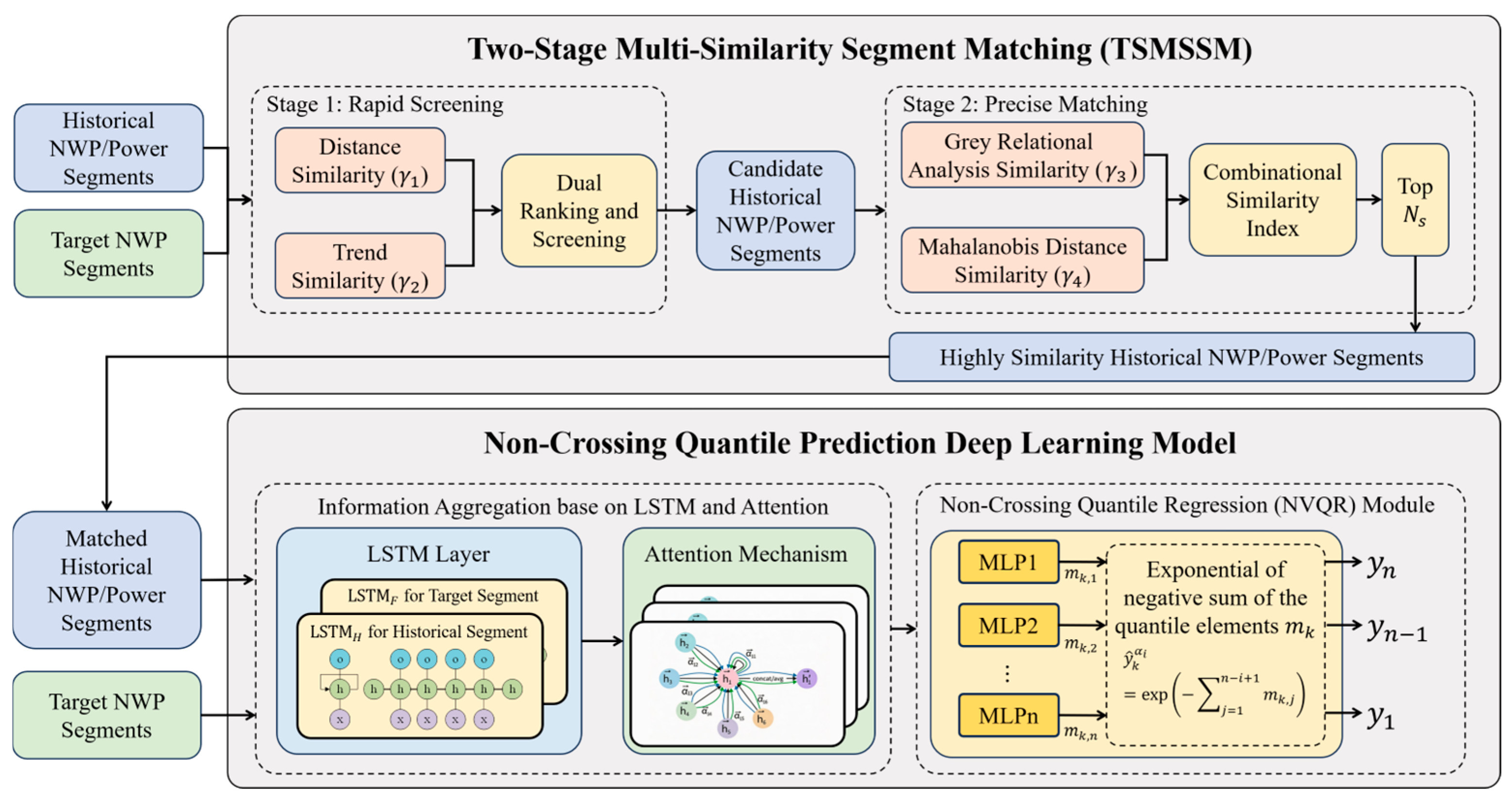
Figure 1. Overall framework of the proposed short-term wind power non-crossing quantile prediction based on two-stage multi-similarity hybrid matching.
Processes 14 01310 g001
Figure 2. Overall framework of proposed TSMSSM method.
Processes 14 01310 g002
Figure 3. Non-crossing quantile prediction neural network structure.
Processes 14 01310 g003
Figure 4. Long Short-Term Memory structure.
Processes 14 01310 g004
Figure 5. Comparison of predicted power between the proposed method and benchmark methods in terms of the power curve.
Processes 14 01310 g005
Table 1. Basic information on the wind power datasets used in this study.
StationTemporal
Resolution
NWP
Information
Power Measurement
Information
PeriodCapacity (MW)
MZ15 minWind speed (m/s, for 10/30/50/70 m)
Wind direction (°, for 10/30/50/70 m)
Temperature (℃)
humidity (%)
air pressure (hPa)
Power Measurement (MW)1 January 2023–30 November 202476
NG90
SJT98
XWZ96
Table 2. Dataset partitioning.
DatasetTime HorizonNumber of Samples
Training set1 January 2023–26 May 2024511
Validation set27 May 2024–13 September 2024109
Testing set14 September 2024–31 December 2024111
Table 3. Forecast segments and history segments.
DatasetNumber of SamplesNumber of Forecast
Segments
Number of History
Segments
Total Number of History Segments
Training set511408811,24213,640
Validation set1098722398
Testing set111888/
Table 4. Hyperparameters of the proposed method used in the experiment.
HyperparameterValueHyperparameterValue
Forecasting Length96Basic Learning Rate0.001
Batch Size128Epochs250
Dropout Rate0.2Early Stopping Patience5
Table 5. Computation time of each matching method.
TSMSSMM1M2
Time spent on single segment0.0618 s3.2238 s17.4764 s
Time spent on validation set42.3249 s2108.37 s>3600 s
Time spent on test set43.1501 s2112.85 s>3600 s
Table 6. Detailed comparison of M1–M4 in the quantile prediction aspect in the evaluation of NCQR module.
StationModelM1M2M3M4
MZpinball0.03850.3910.04310.0386
MRAE0.02320.03920.08290.0273
NAPS0.32260.34660.24540.3209
CRPS0.06470.06570.07260.0649
NGpinball0.03640.03810.03890.0365
MRAE0.02520.04330.07980.0383
NAPS0.33350.34460.27280.3481
CRPS0.06130.06400.06530.0613
SJTpinball0.03820.03870.04060.0382
MRAE0.01210.02830.03370.0139
NAPS0.33280.33670.30090.3331
CRPS0.06440.06510.06700.0642
XWZpinball0.03980.04070.04400.0400
MRAE0.01170.01400.01820.0108
NAPS0.33370.33870.29730.3370
CRPS0.06680.06850.06940.0672
The best and second-best results are highlighted in bold and underlined, respectively.
Table 7. Detailed comparison of proposed model, MLP, LSTM, CNN-LSTM, CNN-XMFR, INCQR and EDNQR in the deterministic prediction.
Station ProposedMLPLSTMCNN-LSTMCNN-XMFRINCQREDNQR
MZMAE (%)9.739.8810.009.819.859.849.79
RMSE (%)14.8215.0615.1815.0115.1614.9514.94
R2 (%)63.1360.0261.3561.9461.4862.5062.92
NGMAE (%)9.219.579.729.249.259.449.35
RMSE (%)14.1414.4914.8614.2814.1314.4914.12
R2 (%)62.3761.5058.3462.2962.2260.3860.29
SJTMAE (%)9.519.8610.039.649.809.839.87
RMSE (%)14.1514.4614.7614.2714.6114.4314.48
R2 (%)62.0660.4058.7761.6859.5660.5860.27
XWZMAE (%)10.0810.3710.5210.1510.5810.3510.21
RMSE (%)16.2716.7316.7916.4717.2116.6316.42
R2 (%)59.4657.1456.8258.6754.6457.6758.47
The best and second-best results are highlighted in bold and underlined, respectively.
Table 8. Detailed comparison of proposed model, MLP, LSTM, CNN-LSTM, CNN-XMFR, INCQR and EDNQR in the quantile prediction.
Station ProposedMLPLSTMCNN-LSTMCNN-XMFRINCQREDNQR
MZpinball0.03730.03880.03920.03850.03940.03860.0391
MRAE0.02310.01330.01320.02680.04850.03350.0381
NAPS0.31200.33690.34110.31210.26560.32780.3225
CRPS0.06430.06520.06590.06470.06610.06490.0658
NGpinball0.03610.03700.03820.03640.03680.03730.0375
MRAE0.02570.05970.02060.04110.04770.03350.0375
NAPS0.31950.34410.34360.33840.35730.33350.3177
CRPS0.06090.06210.06420.06110.06160.06260.0630
SJTpinball0.03760.03860.03920.03800.04010.03840.0386
MRAE0.01230.02670.01660.02080.05260.02170.0204
NAPS0.32140.34720.33930.33270.42140.34110.3472
CRPS0.06260.06490.06600.06330.06740.06460.0650
XWZpinball0.03960.04070.04130.03970.04220.04060.0402
MRAE0.01240.04250.01000.01330.01400.01400.0151
NAPS0.33720.35830.35840.35410.34820.34820.3417
CRPS0.06650.06850.06950.06650.06830.06830.0676
The best and second-best results are highlighted in bold and underlined, respectively.
Table 9. Detailed comparison of proposed model, M1–M3, in the quantile prediction aspect in the module ablation experiment.
Station ProposedM1M2M3
MZpinball0.0373 *0.03850.0390 *0.0383 *
MRAE0.0231 *0.02320.0439 *0.0278
NAPS0.3120 *0.32260.32890.3190 *
CRPS0.0643 *0.06470.0654 *0.0644 *
NGpinball0.0361 *0.03640.0388 *0.0362 *
MRAE0.02570.02520.0706 *0.0370 *
NAPS0.3195 *0.33350.29280.3384 *
CRPS0.0609 *0.06130.06430.0609 *
SJTpinball0.0376 *0.03820.03960.0382
MRAE0.01230.01210.0297 *0.0138
NAPS0.3214 *0.33280.31000.3235 *
CRPS0.0626 *0.06440.0668 *0.0639 *
XWZpinball0.0396 *0.03980.0407 *0.0398 *
MRAE0.01240.01170.01820.0172
NAPS0.33720.33370.32250.3413
CRPS0.0665 *0.06680.0685 *0.0668 *
The best and second-best results are highlighted in bold and underlined, respectively. Metrics marked with an asterisk denote that the model incorporating the TSMSSM module outperforms its counterpart without it.
Disclaimer/Publisher’s Note: The statements, opinions and data contained in all publications are solely those of the individual author(s) and contributor(s) and not of MDPI and/or the editor(s). MDPI and/or the editor(s) disclaim responsibility for any injury to people or property resulting from any ideas, methods, instructions or products referred to in the content.