Article

Investigation of Critical Liquid-Carrying Flow Rates Across Various Sections in Horizontal Gas Wells


1
School of Petroleum Engineering, Xi’an Shiyou University, Xi’an 710065, China
2
School of Economics, North Minzu University, Yinchuan 750021, China
3
Xi’an Economic Development No.1 School, Xi’an 710000, China
4
School of Mechanical Engineering, Xi’an Shiyou University, Xi’an 710065, China
*
Author to whom correspondence should be addressed.
Processes 2026, 14(8), 1292; https://doi.org/10.3390/pr14081292
Submission received: 14 March 2026 / Revised: 10 April 2026 / Accepted: 14 April 2026 / Published: 17 April 2026
(This article belongs to the Section Petroleum and Low-Carbon Energy Process Engineering)

Abstract

To address the challenges of complex wellbore trajectories in horizontal gas wells and the significant differences in droplet entrainment laws across various well sections, which make it difficult to accurately predict the most critical location for liquid loading, this study establishes a prediction model for the critical liquid-carrying flow rate in different well sections. The model is based on droplet force balance and Kelvin–Helmholtz wave theory, considering droplet deformation and energy losses due to wall collisions and friction. By integrating the critical liquid-carrying flow rate models for each section with a four-field coupled wellbore prediction model, a coupled temperature-pressure and liquid-carrying prediction model is developed. Sensitivity analysis was performed on factors influencing the critical liquid-carrying flow rate, and a field data analysis was conducted on 43 gas wells. The results indicate that the proposed model provides accurate predictions, with only one well being misjudged. For four wells near the liquid loading state, the predictions were within a ±15% error range, with an average deviation of only 5.9%. The research results provide a theoretical basis for the accurate prediction of liquid loading in horizontal gas wells.

1. Introduction

Horizontal wells have been widely used in major gas fields worldwide due to their large drainage area, high gas production efficiency, and thorough reservoir stimulation. Horizontal well technology is becoming one of the most economical and effective methods for natural gas development [1,2]. As gas field development progresses, reservoir energy depletes, gas production rates decline, and bottom-hole pressure losses increase, leading to insufficient liquid-carrying capacity. When the gas production rate drops below a certain threshold (the critical liquid-carrying flow rate), the produced gas cannot carry the liquid to the wellhead. The unrecovered liquid accumulates in the wellbore, forming liquid loading, which damages the gas-phase permeability of the near-wellbore region and leads to a significant decline in production or even shut-in due to water flooding [3,4]. Accurately predicting liquid loading and implementing timely drainage measures are of great significance for ensuring efficient gas reservoir development and extending the life cycle of gas wells.
In the full wellbore of a horizontal well, liquid exists primarily in the form of droplets in the gas core and liquid films on the inner wall. Droplet fallback or liquid film reversal is typically used as the criterion for determining the critical gas flow rate. Turner [5] compared and analyzed the droplet and liquid film transport modes, noting that the migration effect of high-speed gas flow on droplets is more consistent with the mechanism of liquid loading in gas wells. For vertical wells under high gas–liquid ratio conditions, he established a spherical droplet model by setting the critical Weber number to 30 and the drag coefficient to 0.44, adjusting the calculated value upward by 20% to represent the actual liquid-carrying flow rate. Based on Turner’s theory, Coleman [6] studied gas wells with wellhead pressures below 3.5 MPa and argued that the Turner model is more accurate without the 20% upward adjustment. Li [7] suggested that during the transport process, droplets are more likely to deform into ellipsoidal shapes due to the velocity pressure generated by high-speed gas flow. Based on the Turner model, Li established an ellipsoidal droplet model with a drag coefficient of 1.0. Based on extensive experimental results, Wang [8] found that the droplet morphology is spherical-cap shaped; by setting the drag coefficient to 1.13, he modified the Turner model to establish a spherical-cap droplet model. As droplets deform under the action of gas flow, their projected area and maximum diameter change, leading to variations in the drag coefficient and critical Weber number. Assuming model coefficients as constants leads to certain limitations. Consequently, Wang [9] constructed a functional relationship between droplet deformation parameters and the critical Weber number based on the particle balance principle and energy conservation equations, establishing a droplet model for critical liquid carrying that accounts for changes in shape and size. Li [10] introduced characteristic parameters to establish a critical liquid-carrying flow rate model considering droplet size and deformation, comparing it with Turner’s [5] and Li’s [7] models and explaining the discrepancies between existing models through these characteristic parameters. However, the aforementioned models assume droplet motion in vertical wells, which limits their application in inclined and horizontal wells. Therefore, Belfroid [11] considered the influence of pipe inclination on droplet forces and proposed a prediction model for critical liquid-carrying flow rates in inclined wells, covering an inclination range of 5° to 90°. Li [12] argued that the trajectory of droplets in inclined wellbores does not always follow the wellbore axis but shifts toward the pipe wall, eventually sliding upward along the wall. By introducing a friction coefficient and inclination angle, the critical liquid-carrying model was modified. Ming [13] performed a nonlinear fitting of the relationship between the Reynolds number and drag coefficient under turbulent conditions and established a new prediction model for the continuous critical liquid-carrying flow rate in directional wells under gas-phase turbulence. The relative error of this model is less than 10%, improving accuracy by 10.416% to 66.125% compared to commonly used models.
Regarding the flow distribution of the liquid film in the wellbore, Wallis [14] first proposed a criterion for liquid film reversal in vertical wells, but this method did not consider the impact of fluid physical properties. Based on the Wallis model, Richter [15] considered the pipe diameter factor and proposed a liquid film calculation model suitable for large pipe diameters. Barnea [16] proposed a critical liquid-carrying model for uniform liquid film distribution in inclined wells. However, under actual conditions, inclined pipe flow exhibits obvious radial gradient distribution characteristics, with liquid film accumulation at the bottom of the pipe, leading to limitations in this model. Luo [17] considered the influence of the inclination angle on the non-uniform radial distribution of the liquid film based on the Barnea model and established expressions for non-uniform liquid film thickness under different angles using experimental data. Based on experimental data from Guner and Alassdi, Li [18] argued that the liquid film thickness at the bottom is greatest at an inclination angle of 30° and modified Luo’s formula for calculating liquid film thickness. Wang [19] studied the relationship between the bottom liquid film thickness and the gas–liquid interfacial friction coefficient in inclined wells, provided an empirical formula for calculating the maximum liquid film thickness based on experimental data, and proposed a new model for non-uniform liquid film distribution based on the principle of force balance. Sun [20] proposed correlation relationships for gas–liquid interfacial roughness in vertical annular flow with and without disturbance waves, clearly explaining the influence of fluctuating liquid films on interfacial shear stress. Based on Newton’s law of internal friction and gas–liquid two-phase force balance, Yu [21] established a critical liquid-carrying model for directional wells based on the liquid film reversal mechanism, noting that in inclined wells, the gas–liquid two-phase flow exhibits stratified flow, with the liquid distributed along the pipe wall in the form of a liquid film. Liu [22] conducted a force analysis of gas–liquid two-phase flow in the wellbore based on the annular-mist flow liquid film theory and established a critical liquid-carrying flow rate prediction model that comprehensively considers the effects of fluid flow regimes and liquid film thickness on the friction coefficient. Xie [23] proposed a new calculation method for the droplet entrainment rate under the influence of chokes in their study of tight sandstone water-producing gas wells and developed a mechanistic prediction model for the critical liquid-carrying gas velocity in gas wells with downhole chokes.
In summary, existing critical liquid-carrying flow rate models often use the temperature and pressure at the wellhead or bottom-hole for calculations. However, as the liquid phase is carried from the bottom to the wellhead, the wellbore temperature and pressure change continuously. Assuming constant values for these parameters introduces errors. Furthermore, horizontal wells have complex structures consisting of horizontal, inclined, and vertical sections, and the movement laws of the liquid phase vary significantly across these sections. To accurately predict the liquid loading state of horizontal gas wells, this study couples the critical liquid-carrying models for different well sections with a four-field wellbore prediction model to establish a coupled temperature-pressure and liquid-carrying prediction model.

2. Mathematical Model

2.1. Critical Liquid-Carrying Flow Rate Model

The liquid-carrying model for the vertical well section adopts the droplet model. A gas well can continuously carry liquid and maintain production only when the largest droplets are transported out of the wellhead by the gas. During the movement of the droplet, the pressure difference between its windward and leeward sides causes the droplet to deform, leading to an increase in the windward area and the drag coefficient. Furthermore, the surface free energy of the droplet also increases. Assuming the total turbulent kinetic energy of the gas phase remains constant, the maximum droplet diameter increases accordingly.
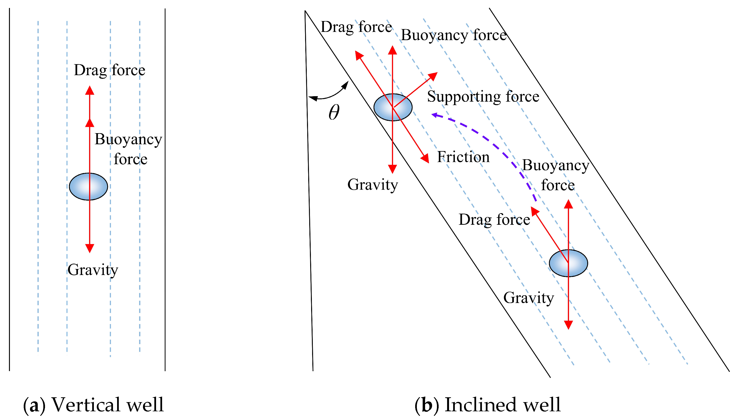
Assuming the droplet is in a critical state, it is primarily subjected to three forces: the buoyancy force from the surrounding gas, its own gravity, and the drag force exerted by the gas. The force analysis is illustrated in Figure 1. Based on the principle that the net force acting on the droplet along the gas flow direction is zero, the following is obtained:
F D + F B F G = 0
F D = 1 2 C d A v c 1 2 ρ g
F B = ρ g g V
F G = ρ l g V
where FD is the gas drag force acting on the droplet, N; FB is the buoyancy force exerted by the gas on the droplet, N; FG is the gravity of the droplet, N; Cd is the drag coefficient, dimensionless; V is the droplet volume, m3; A is the windward area of the droplet, m2; ρg is the gas density, kg/m3; ρl is the liquid density, kg/m3; vc1 is the critical liquid-carrying velocity in the vertical section, m/s; and g is the gravitational acceleration, m/s2.
Rearranging the equations yields the formula for the critical liquid-carrying velocity in the vertical well section:
v c 1 = ρ l g V ρ g g V 1 2 C d A ρ g
Assuming that after deformation, the windward diameter of the droplet is k times its original diameter, the relationship is given by:
V A = 1 6 π d 3 1 4 π d 1 2 = 2 d 3 k 2
where d is the original droplet diameter, m; d1 is the deformed droplet diameter, m; and k is the droplet deformation coefficient, where k = d1/d.
After the droplet deforms, its maximum diameter can be determined according to the definition of the critical Weber number:
d max = σ W e c ρ g v c 1 2
where dmax is the maximum droplet diameter, m; Wec is the critical Weber number, dimensionless; and σ is the gas-water interfacial tension, N/m.
Substituting Equations (6) and (7) into Equation (5), the relationship for the critical liquid-carrying velocity considering droplet deformation is obtained as:
v c 1 = C k , W e c σ ρ l ρ g ρ g 2 0.25
where
C k , W e c = 4 g W e c 3 C d k 2 0.25
The forces acting on a droplet in an inclined well differ from those in a vertical well. The drag force exerted on the droplet acts along the direction of the wellbore and can be decomposed into horizontal and vertical components. Under the action of the horizontal component of the drag force, the droplet moves horizontally until it collides with the pipe wall, after which it is carried out of the wellbore at a certain velocity. During this process, the droplet is primarily subjected to the combined effects of drag force, buoyancy, gravity, friction, and normal support force. The force analysis is shown in Figure 2.
According to Newton’s second law, when the droplet motion reaches the critical state, the force balance relationship along the gas flow direction can be expressed as:
F D + F B F G cos θ = 0
The drag force, buoyancy force, and gravity exerted on the droplet are respectively given by:
F D = 1 2 C d A v c 2 2 ρ g
F B = ρ g g V
F G = ρ l g V
Rearranging the terms yields the formula for the critical liquid-carrying flow velocity of the gas well:
v c 2 = cos θ ρ l g V ρ g g V 1 2 C d A ρ g
Based on the definitions of droplet deformation and the critical Weber number, substituting Equations (6) and (7) into Equation (14) yields the relationship for the critical liquid-carrying flow velocity considering the inclination angle:
v c 2 = C k , W e c σ ρ l ρ g ρ g 2 0.25
where
C k , W e c = 4 g W e c cos θ 3 C d k 2 0.25
The critical gas flow velocity is calculated using Equation (15), and the calculated vc is subsequently used to compute the effective velocity, as shown below:
v eff = v c 2 + v sp
where veff is the effective migration velocity, m/s; vc2 is the critical gas velocity in theinclined well section, m/s; and vsp is the additional velocity above the critical velocity required to maintain the critical state after rebound, m/s.
The energy loss caused by droplet collisions with the pipe wall is related to the well deviation rate, increasing as the incidence angle between the pipe wall and the droplet increases. By fitting the energy loss against the incidence angle, where the experimental impact angles range from approximately 10° to 60° and the fractional energy loss converges to a theoretical upper limit of 95% when the impact angle exceeds 70°, the following fitted equation is obtained [24]:
v c 2 2 v sp 2 v c 2 2 = 0.0406 × θ i 0.7537
where θi is the incident angle at which the droplet collides with the pipe wall, (°).
The recovery velocity of the droplet after colliding with the pipe wall is determined by the energy loss coefficient α, followed by the determination of the drag force acting on the droplet under the new equilibrium condition:
F d = α 2 C d ρ g π ρ g k 2 v c 2 8 = α 2 F d
where
v sp v c 2 = α
To ensure that the droplet can still be carried by the gas after the collision, a compensation drag force must be determined to compensate for the energy loss of the droplet after colliding with the pipe wall. Its expression is as follows:
F sp = F d F d = ( 1 α 2 ) F d
where F sp is the compensation drag force, N; and F d is the aerodynamic drag force acting on the droplet after collision with the pipe wall, N.
The compensation velocity is obtained from the compensation drag force:
v sp 2 = 1 α 2 v c 2 2
v sp = β v c 2
where β is the droplet collision coefficient, dimensionless.
Substituting Equation (23) into Equation (17) and incorporating the compensation velocity into the critical velocity allows the effective velocity in the inclined well section to be calculated:
v eff = v c + β v c 2
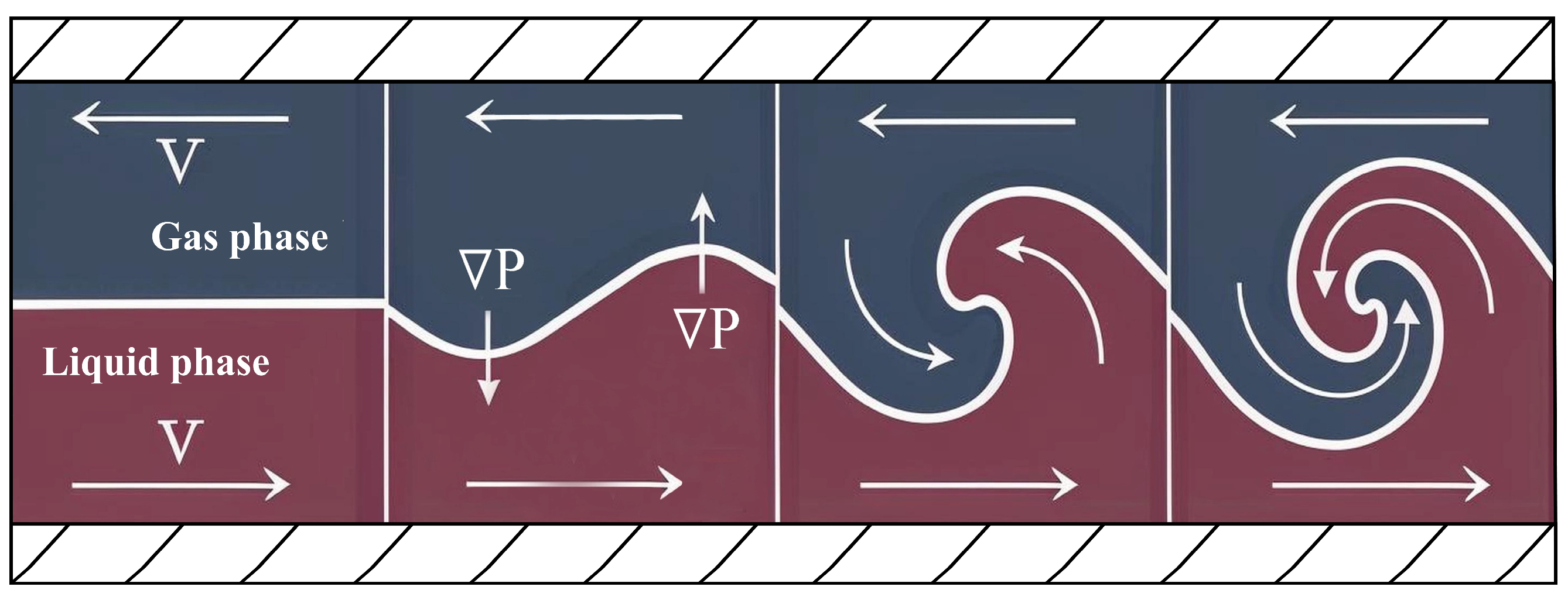
In the horizontal section, liquid typically exists in the form of a liquid film attached to the pipe wall. As the kinetic energy of the gas phase continuously increases, a pressure difference gradient is generated along the circumferential direction of the pipe. Based on the Kelvin–Helmholtz wave theory, when the suction force generated by the pressure gradient overcomes the gravity that stabilizes the interfacial wave, the K-H instability effect occurs. As the gas flow rate continues to increase, the unstable waves at the interface cause the liquid film to move around the pipe wall, thereby resulting in droplet entrainment, as shown in Figure 3.
Lin and Hanratty [25] assumed that the gas-phase and liquid-phase flows are composed of a mean flow and a perturbation. Combining the linear momentum equations for the two phases yields:
k ρ l ( v l C ) 2 coth ( k h l ) + k ρ g ( v g C ) 2 coth ( k h g ) = g ( ρ l ρ g ) + σ k 2
where k is the wavenumber of the unstable wave and C is the wave velocity.
Solving Equation (25) yields the relative critical flow velocity when unstable fluctuations occur at the gas–liquid interface:
v g v l c = 2 g σ ρ l ρ g 2 0 . 25
Andritsos and Hanratty [26] proposed that when the gas velocity reaches twice the value required to initiate K-H instability waves, interfacial fluctuations will lead to droplet formation. Neglecting the influence of the liquid phase under high gas–liquid ratio conditions, the formula for the critical liquid-carrying flow velocity in the horizontal section is obtained as:
v c 3 = 2 2 g σ ρ l ρ g 2 0 . 25

2.2. Liquid-Carrying Model Coefficients

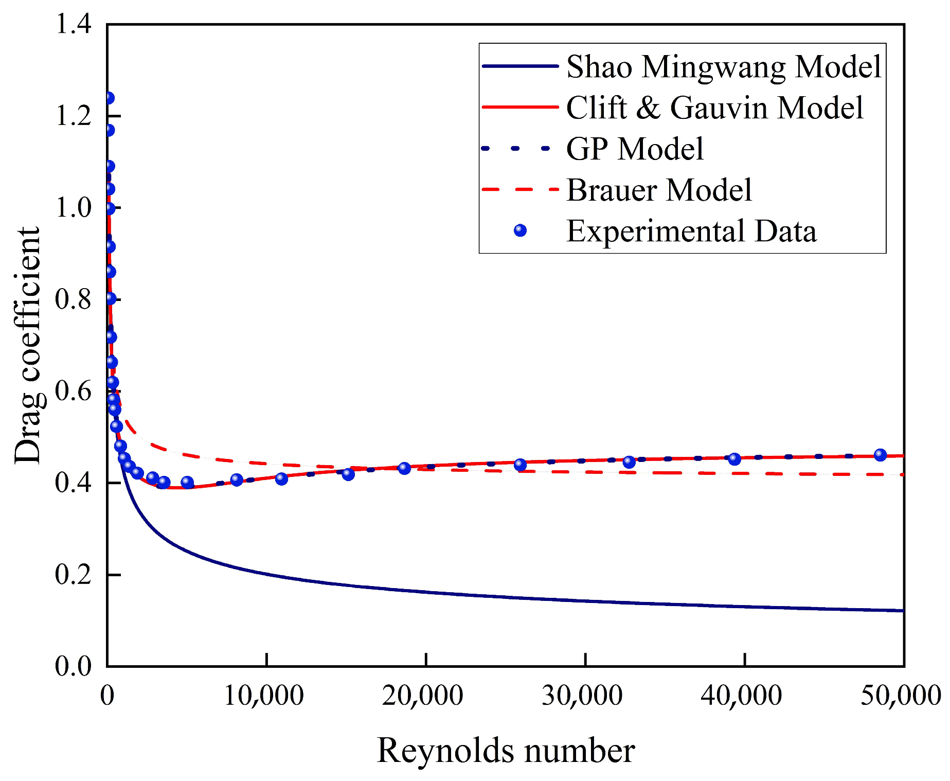
The drag coefficient is dependent on the droplet shape and the Reynolds number (Re). Figure 4 presents the drag coefficient curves calculated using existing empirical models. When Re < 100, the calculated values from all models align well with the experimental data. For 100 < Re < 2000, the results from the GP model and the Clift model closely match the experimental values, the Brauer model exhibits some deviation, and the Shao Mingwang model shows a significant discrepancy from the experimental data. As Re continues to increase, the average error is 29.0% for the Shao Mingwang model, 11.2% for the Brauer model, 2.56% for the Clift & Gauvin model, and 1.97% for the GP model. Therefore, the GP model provides the most accurate calculations.
The aforementioned models derive the drag coefficient based on the assumption of spherical droplets. However, under actual flowing conditions, the droplet interface undergoes deformation due to aerodynamic forces, which correspondingly alter the drag coefficient and the windward area. This leads to a significant deviation between the aerodynamic drag calculated under the traditional spherical assumption and the actual operating conditions. Comprehensively considering the effects of droplet deformation and internal fluid flow [27,28], this study increases the value calculated by the GP model by 15% to serve as the drag coefficient for ellipsoidal droplets, yielding:
C d = 6.30844 × 10 9 tanh ( 4.3774 × 10 9 Re ) + 0.081535 tanh ( 700.6574 Re )                   + 0.44781 tanh ( 74.1539 Re ) 0.13777 tanh ( 7429.0834 Re )                   + 1.97501 tanh ( 9.9851 Re + 2.3348 ) + 0.54556
The critical Weber number determines the maximum entrained droplet diameter. It is necessary to comprehensively consider the effects of both gas and liquid phase velocities on the droplet size. The calculation formula for the critical Weber number of the droplet is given by [29]:
W e c = 5.14 ρ g v sg 2 λ σ 15.4 W e l 0.58 + 3.5 G le ρ l v sg
where
λ = σ ρ l g
W e l = ρ l v sg 2 λ σ
where Wel is the liquid phase critical Weber number, dimensionless; Gle is the mass flux of the droplets, kg/(m2·s).
The droplet deformation parameter is determined by the critical Weber number. By utilizing the Levenberg–Marquardt algorithm and global optimization methods for data fitting, the functional relationship between the critical Weber number and the droplet deformation parameter is proposed as follows:
W e c = 16 [ 2 π ( k 2 4 + 1 2 k ) 7 π 1 k 2 ( k 3 4 + 1 4 k 3 + 5 8 ) 2 k 2 + 13 2 k + 29 4 k 4 π ] 7.951 2.774 k 2 + 0.3077 k 5.117 k + 0.501 k 2
During the droplet entrainment process by the gas phase, the interfacial tension serves as a crucial physical property, and its values are significantly influenced by the wellbore temperature and pressure. Therefore, this study adopts a surface tension calculation model that accounts for the effects of pressure and temperature [30]. The correlations are as follows:
σ T = 1.8 137.78 T 206 σ 23.33 σ 137.78 + σ 137.78
σ 23.33 = 76 exp 0.0362575 p
σ 137.78 = 52.5 0.87018 p

2.3. Four-Field Coupled Model

Considering the complexity of the flow and heat transfer in the gas storage wellbore, the following assumptions are made:
(1)
The heat transfer media exhibit an axisymmetric configuration centered on the tubing, with all materials treated as thermally isotropic.
(2)
Wellbore flow is considered one-dimensional, and axial heat conduction is neglected.
(3)
Constant gas injection and production rates are maintained at the wellhead.
(4)
The wellbore fluid is initially static and in thermal equilibrium with the surrounding formation prior to operational phases.
Based on the above assumptions, the four-field coupled governing equations of the gas storage well are established as follows [31,32]:
T z = C J ( v 2 d ρ d z f ρ v 2 2 d ± ρ g cos θ ) + ( L ( T e T ) + v 2 ρ d ρ d z ± g cos θ ) / C p
d p d z = ± ρ g cos θ f ρ v 2 2 d + v 2 d ρ d z
d v d z = v ρ d ρ d z
d ρ d z = ( M R Z ( ± ρ g cos θ f ρ v 2 2 d ) + ( ρ L ( T e T ) ± ρ g cos θ ) / C p ) / ( T + v 2 ( 1 C p M R Z ) )
The initial conditions for the governing equations are prescribed by:
p ( z 0 ) = p 0 ,   T ( z 0 ) = T 0 ,   ρ ( z 0 ) = M p 0 / R Z ,   v ( z 0 ) = w / A ρ ( z 0 )
Meanwhile, the solution is subject to the following boundary conditions:
T e = T bottom g G ( H z )
where Cp is the specific heat of the fluid, J/(kg·°C); T is the wellbore gas temperature, °C; CJ is the Joule-Thomson coefficient, K/Pa; Te is the formation temperature, °C; Tsurf is the surface temperature, °C; Tbottom is the bottom hole temperature, °C; H is the well depth, m; gG is the geothermal gradient, °C/m; L is the relaxation distance, 1/m; v is the gas velocity, m/s; θ is the wellbore inclination, (°); p is the wellbore gas pressure, Pa; w is the gas mass flow rate, kg/s; ρ is the wellbore gas density, m3/kg; M is the relative molecular mass of the natural gas mixture, dimensionless; g is the gravitational acceleration, m/s2; f is the friction coefficient between the fluid and the tubing, dimensionless; Z is the gas compressibility factor, dimensionless; R is the ideal gas constant, 8.314 J/(mol·°C).

2.4. Coupling of Temperature, Pressure, and Liquid-Carrying Flow Rate

By integrating the section-specific critical liquid-carrying flow rate prediction models with the temperature and pressure field prediction models, a coupled temperature-pressure and liquid-carrying prediction model is established. The specific solution procedure is detailed as follows:
(1)
Assume the pressure and temperature profiles for the horizontal section to calculate the temperature and pressure distribution of the natural gas within the wellbore.
(2)
Based on the temperature and pressure distribution in the horizontal section, calculate the natural gas density, viscosity, compressibility factor, and gas-water interfacial tension, and then solve for the distribution of the critical liquid-carrying flow rate across the horizontal section.
(3)
Using the temperature, pressure, and natural gas physical properties at the heel of the horizontal section as the initial values for the inclined section, assume the pressure and temperature profiles for the inclined section to calculate the gas temperature and pressure distribution within the wellbore.
(4)
Based on the temperature and pressure distribution in the inclined section, calculate the natural gas density, viscosity, compressibility factor, and gas-water interfacial tension, and then solve for the distribution of the critical liquid-carrying flow rate across the inclined section.
(5)
Using the temperature, pressure, and natural gas physical properties at the terminal end of the inclined section as the initial values for the vertical section, assume the pressure and temperature profiles for the vertical section to calculate the gas temperature and pressure distribution within the wellbore.
(6)
Based on the temperature and pressure distribution in the vertical section, calculate the natural gas density, viscosity, compressibility factor, and gas-water interfacial tension, and then solve for the distribution of the critical liquid-carrying flow rate across the vertical section.
(7)
Compare the critical liquid-carrying flow rates across the different well sections to determine the maximum critical liquid-carrying flow rate.

3. Results

3.1. Analysis of Critical Liquid-Carrying Behavior in Different Well Sections

Based on the critical liquid-carrying flow rate models for different well sections, a comparative analysis is conducted on the critical liquid-carrying behavior and its influencing factors across these sections. Pressure variations affect the ability of the gas to carry droplets, temperature changes influence the production status and liquid loading conditions of the wellbore, and the pipe diameter reflects the flow resistance distribution of the liquid-carrying system. Therefore, combining actual production conditions, a comparative analysis is performed on influencing factors such as wellbore temperature, pressure, and pipe diameter.
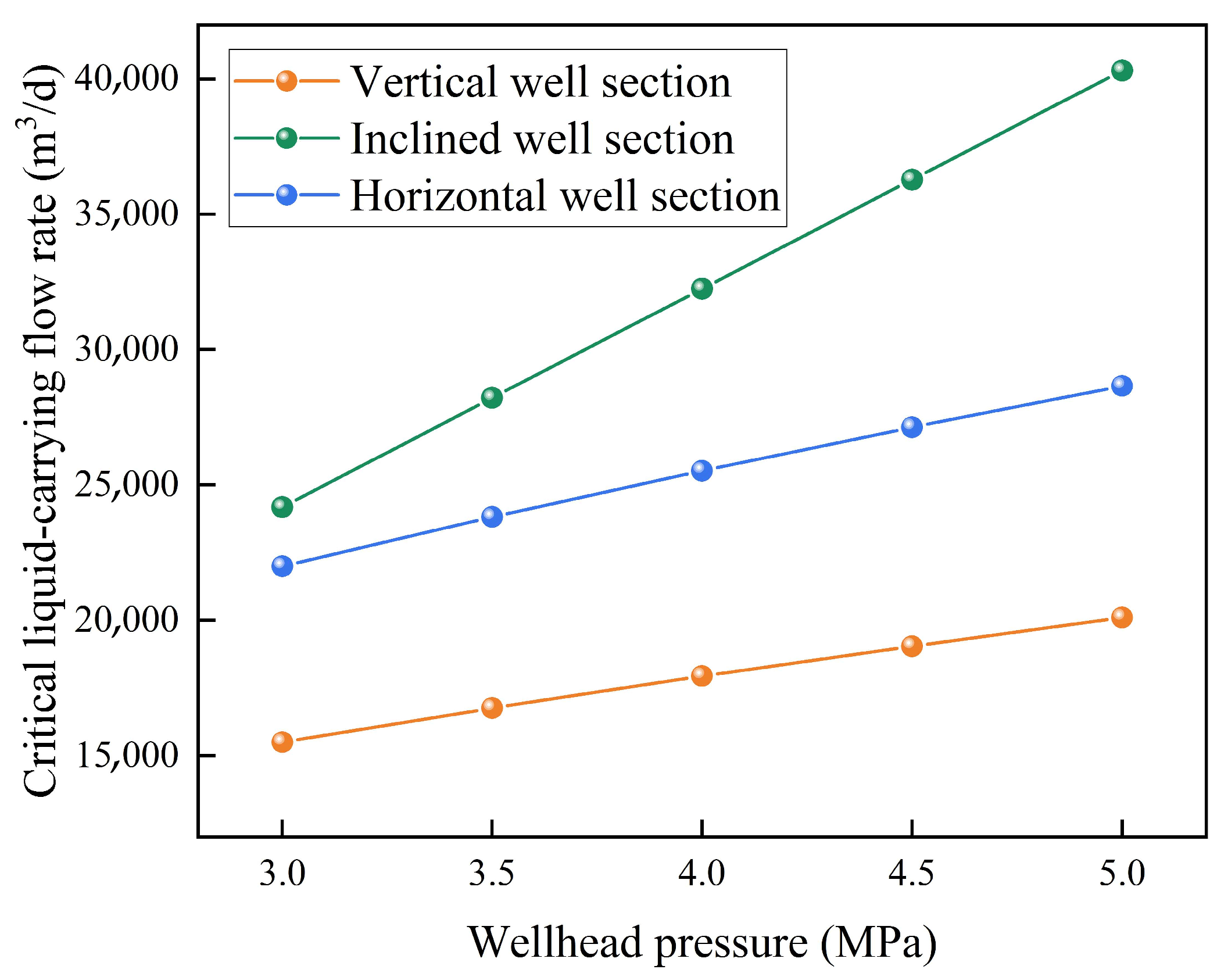
Fixing the wellhead temperature at 26.8 °C and the tubing inner diameter at 62.0 mm, with the wellhead pressure constrained between 3.0 and 5.0 MPa, the relationship between the critical liquid-carrying flow rate and wellhead pressure for different well sections (vertical, inclined, and horizontal) is obtained, as shown in Figure 5.
As the wellhead pressure increases from 3.0 MPa to 5.0 MPa, the critical liquid-carrying flow rate in the vertical section significantly increases from 15,495 m3/d to 20,097 m3/d, in the inclined section from 24,184 m3/d to 40,306 m3/d, and in the horizontal section from 21,996 m3/d to 28,657 m3/d. This indicates a positive correlation between the critical liquid-carrying flow rate and wellhead pressure. An increase in wellhead pressure leads to a decrease in gas-phase velocity, weakening the liquid-carrying capacity of the gas and accelerating the liquid loading process in the gas well. Therefore, under high wellhead pressure conditions, choke regulation can be utilized to reduce wellhead pressure, and chemical agents can be injected to improve liquid-carrying efficiency.
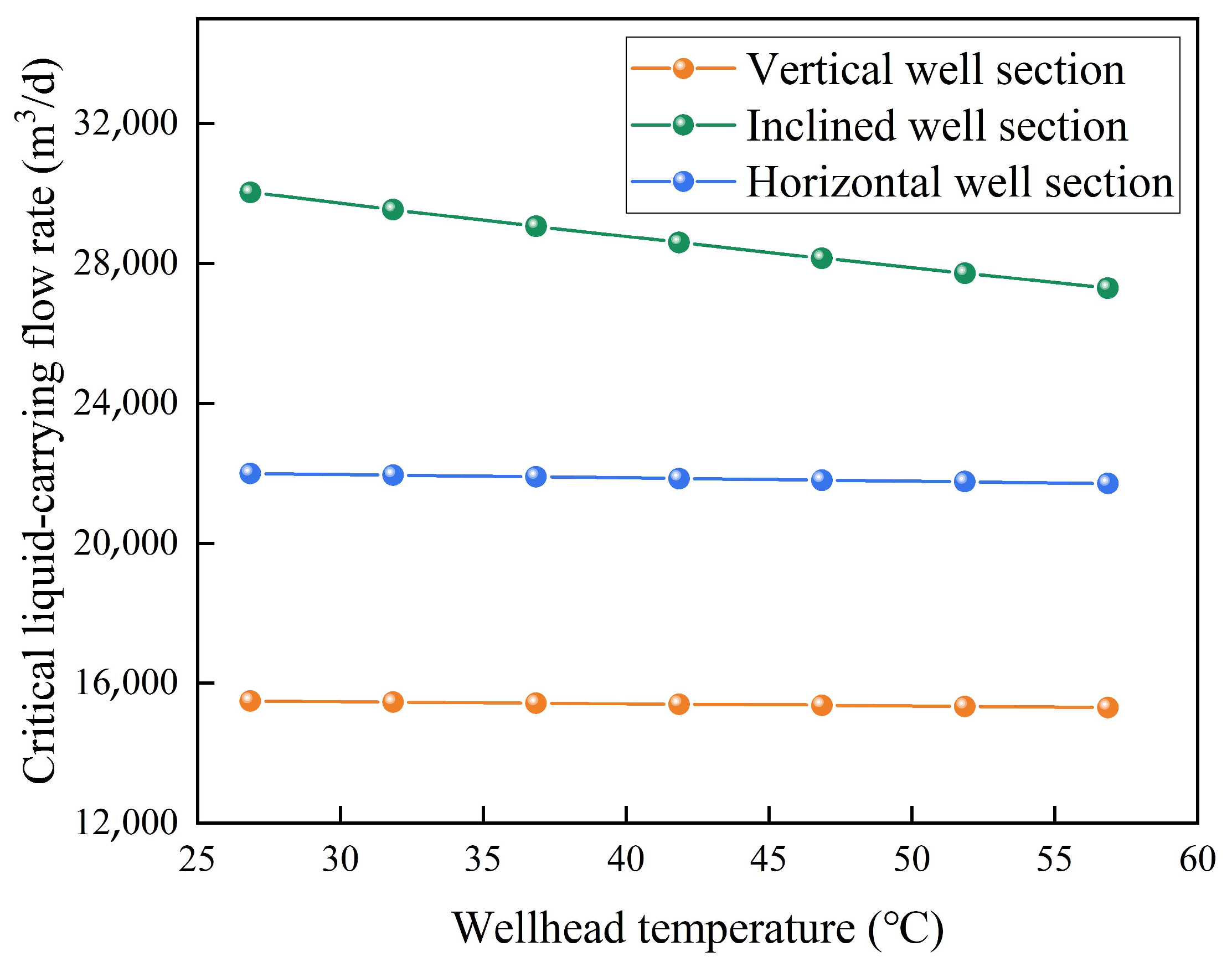
Fixing the wellhead pressure at 3.0 MPa and the tubing inner diameter at 62.0 mm, with the wellhead temperature constrained between 26.8 °C and 56.8 °C, the relationship between the critical liquid-carrying flow rate and wellhead temperature for different well sections is obtained, as shown in Figure 6.
When the wellhead temperature increases from 26.8 °C to 56.8 °C, the critical liquid-carrying flow rate in the vertical section decreases from 15,495 m3/d to 15,305 m3/d, in the inclined section from 30,032 m3/d to 27,302 m3/d, and in the horizontal section from 21,996 m3/d to 21,713 m3/d. This indicates a negative correlation between the critical liquid-carrying flow rate and wellhead temperature. An increase in wellhead temperature promotes the formation of mist flow by reducing gas density, liquid viscosity, and surface tension, thereby enhancing the liquid-carrying capacity of the gas phase and resulting in a lower critical liquid-carrying flow rate. During gas well production, the wellhead choke valve can be dynamically adjusted, or chemical agents can be injected to reduce liquid viscosity, fully utilizing the temperature effect to minimize liquid-carrying energy consumption.
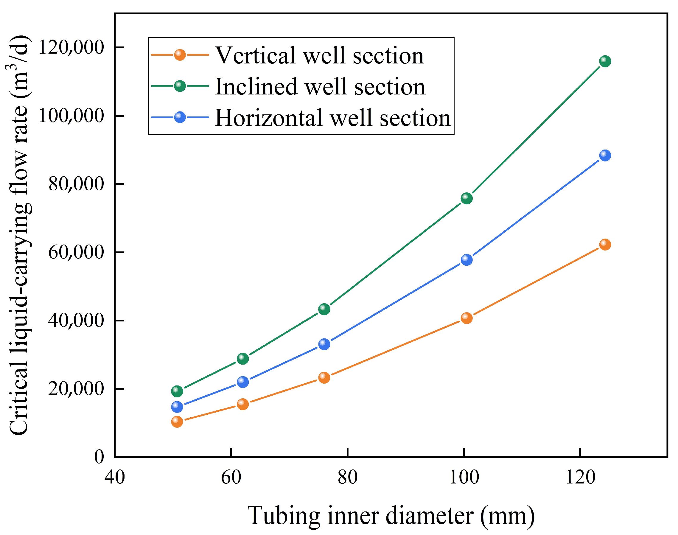
Fixing the wellhead pressure at 3.0 MPa and the wellhead temperature at 26.8 °C, with selected tubing inner diameters of 50.7, 62.0, 76.0, 100.5, and 124.3 mm, the relationship between the critical liquid-carrying flow rate and tubing inner diameter for different well sections is obtained, as shown in Figure 7.
As the tubing inner diameter increases from 50.7 mm to 124.3 mm, the critical liquid-carrying flow rate in the vertical section significantly increases from 10,362 m3/d to 62,283 m3/d, in the inclined section from 19,292 m3/d to 115,960 m3/d, and in the horizontal section from 14,709 m3/d to 88,412 m3/d. This indicates a positive correlation between the critical liquid-carrying flow rate and tubing inner diameter. An increase in the tubing inner diameter leads to a decrease in gas-phase velocity, weakening the shear-carrying effect of the gas on the liquid phase and causing the critical liquid-carrying flow rate to increase. In actual gas well production, throttling technology can be adopted to reduce the flow area of the produced gas, lowering the critical liquid-carrying flow rate and ensuring continuous liquid-carrying production.
Combining Figure 4, Figure 5 and Figure 6, it can be observed that the vertical section has the lowest critical liquid-carrying flow rate, the inclined section has the highest, and the horizontal section falls between the vertical and inclined sections. In the vertical section, the gas flows upward while gravity acts downward; the liquid naturally settles due to gravity, and the gas velocity only needs to overcome the settling velocity of the droplets to effectively carry the liquid phase. In the inclined section, the component of gravity along the wellbore direction causes droplets to migrate toward the pipe wall. Energy losses occur after the droplets collide with the wall and due to frictional resistance as they move along the wall. The gas velocity must overcome droplet gravity, collision-induced energy losses, and friction-induced energy losses to effectively carry the liquid phase. In the horizontal section, the liquid tends to form a liquid film or droplets at the bottom of the pipe wall, requiring a higher gas velocity to be sheared and transported forward, resulting in a critical flow rate that lies between those of the vertical and inclined wells.

3.2. Field Data Analysis

Table 1 compares the common critical liquid-carrying velocity models. Both the Turner model [5] and the Li Min model [7] treat the wellbore as a vertical well; thus, the coefficients in their final model expressions are independent of the inclination angle. The Belfroid model [11] and the Li Li model [12] comprehensively consider the effect of the tubing inclination angle on droplets, establishing angle-corrected prediction models for the critical liquid-carrying flow rate.
The aforementioned models were respectively applied to predict the liquid loading status of 43 field gas wells. Among them, the production data for the 30 vertical wells were sourced from References [5,33], the data for the 11 inclined wells from References [13,34], and the data for the 2 horizontal wells from Reference [35]. The specific data for the 43 wells are listed in Table 2. For any missing relevant data, values were determined based on field experience.
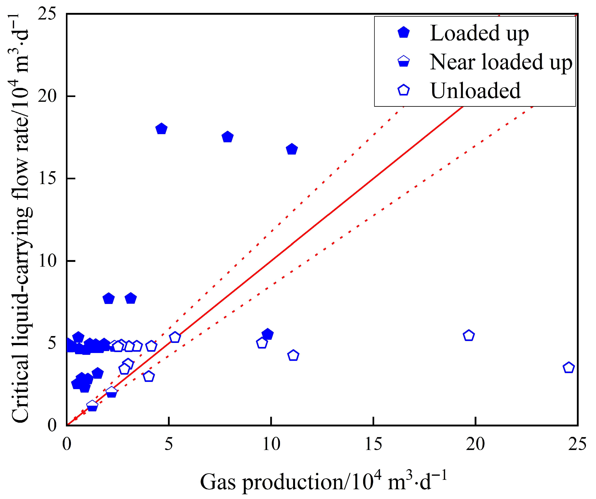
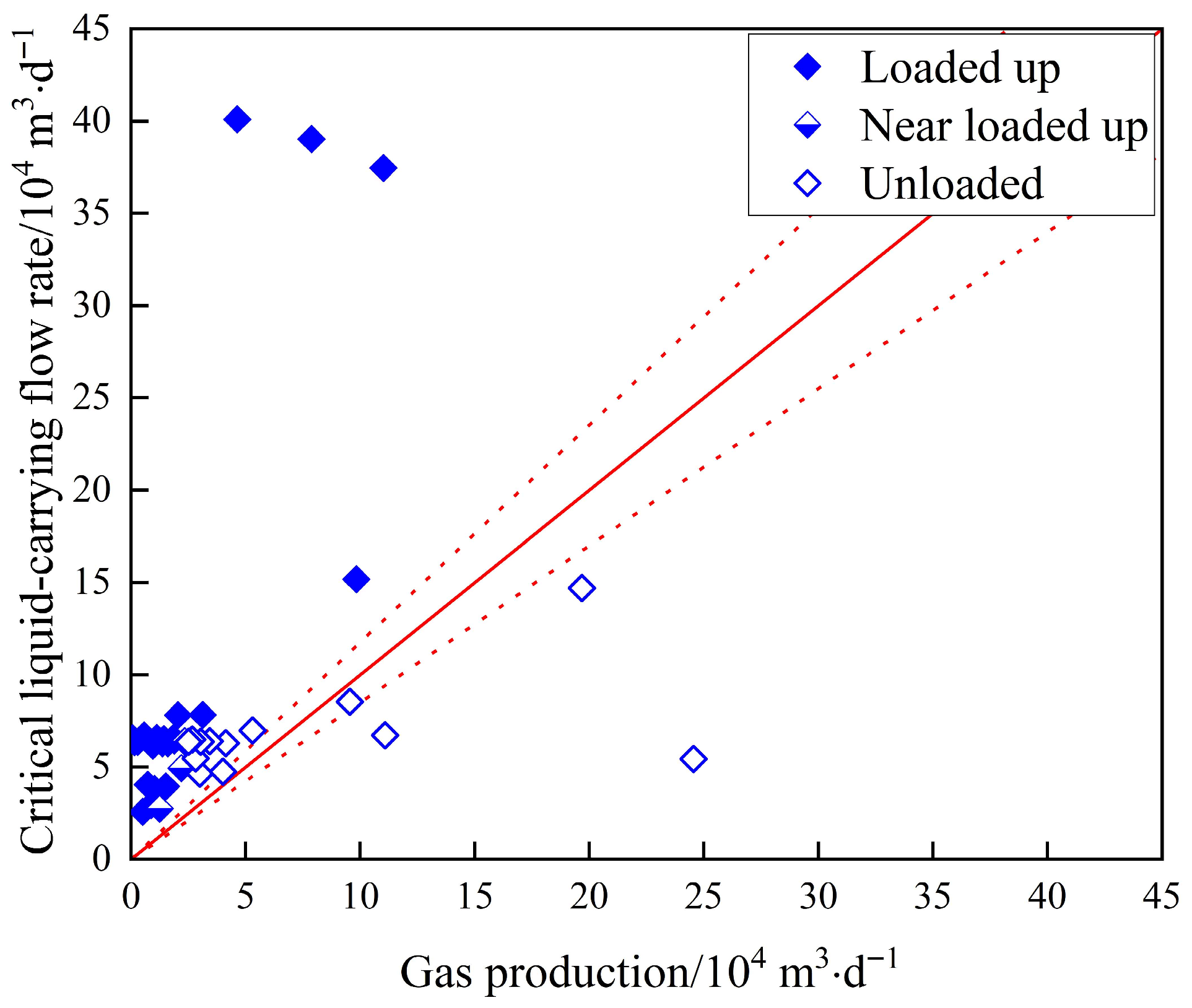
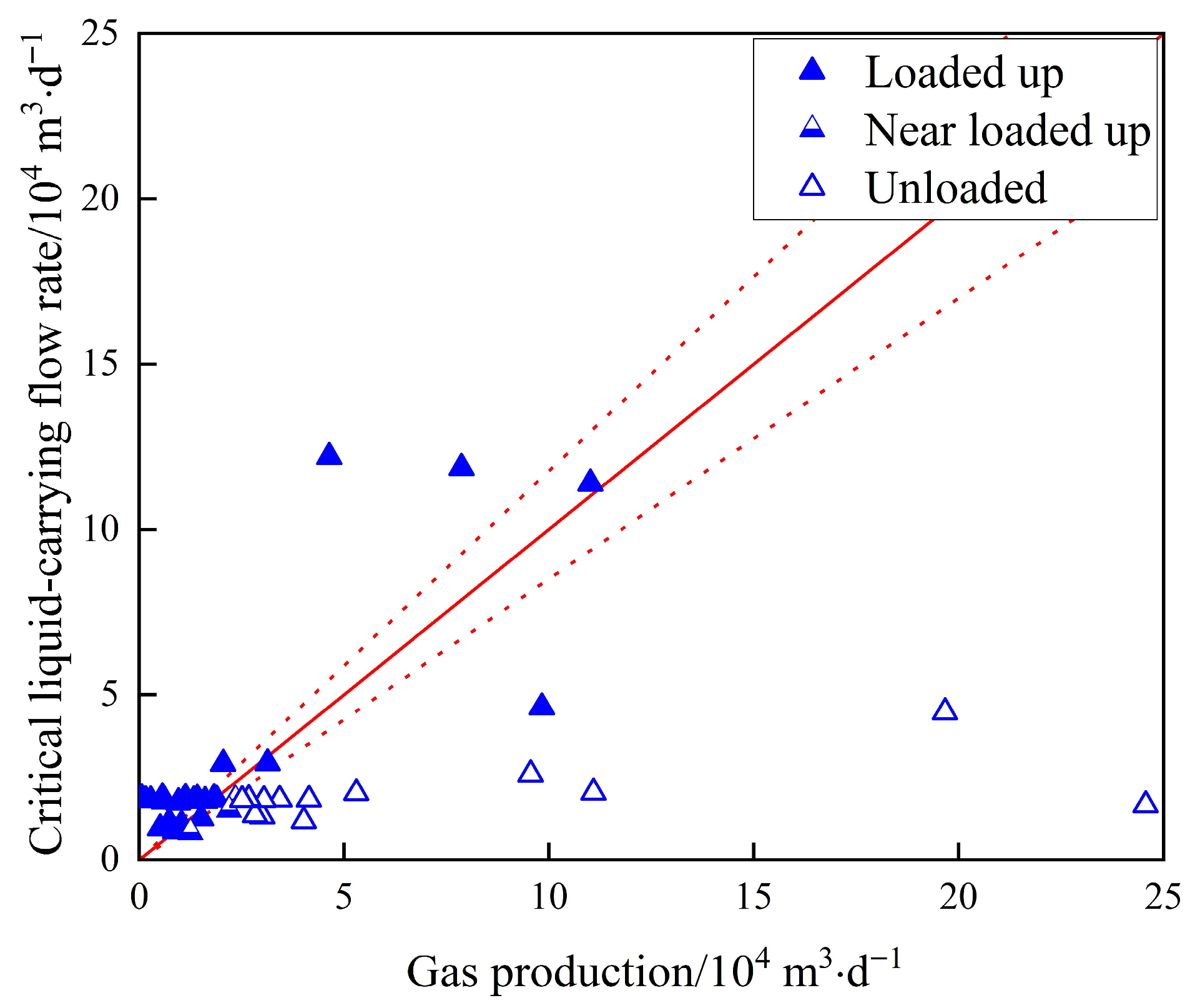
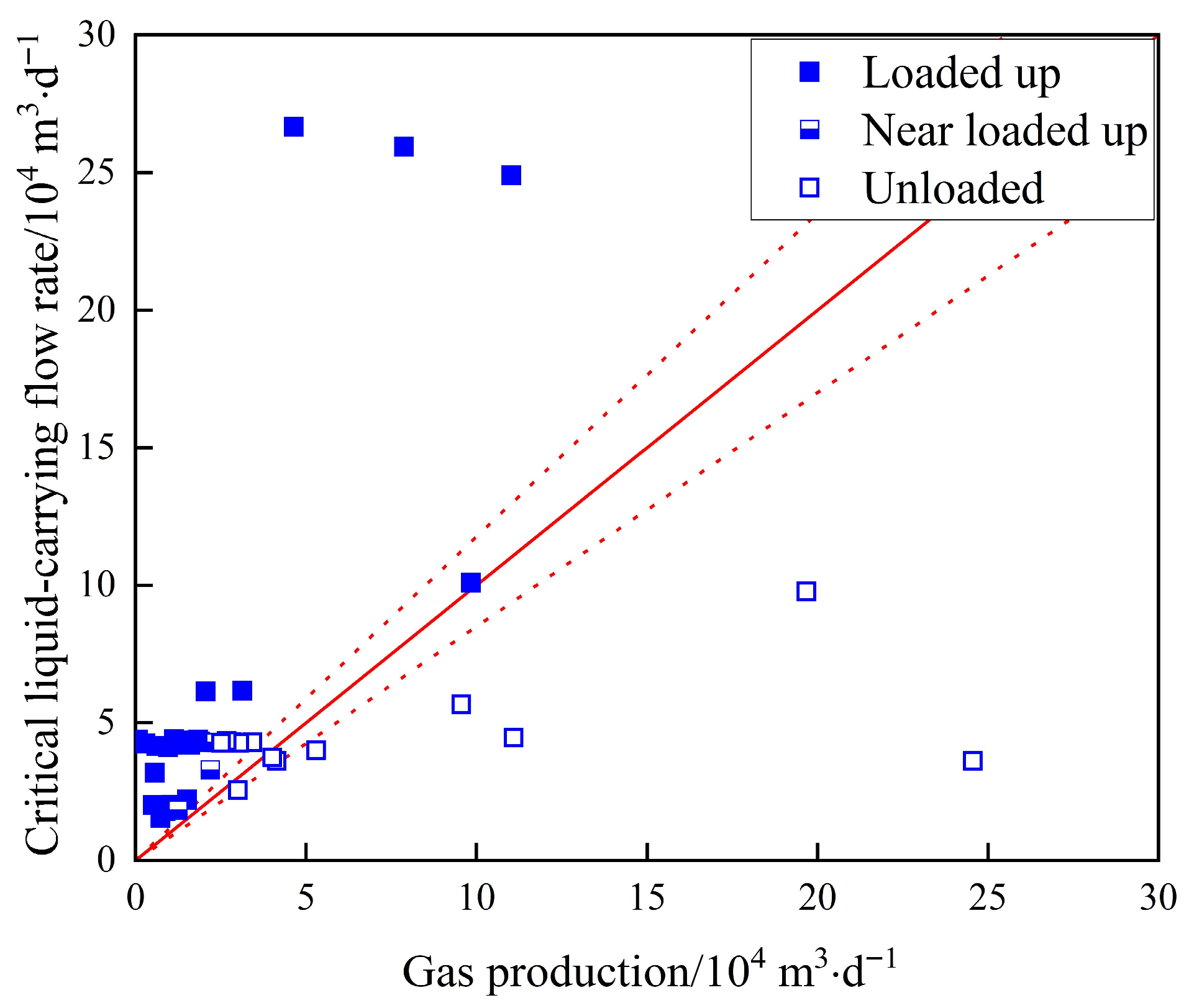
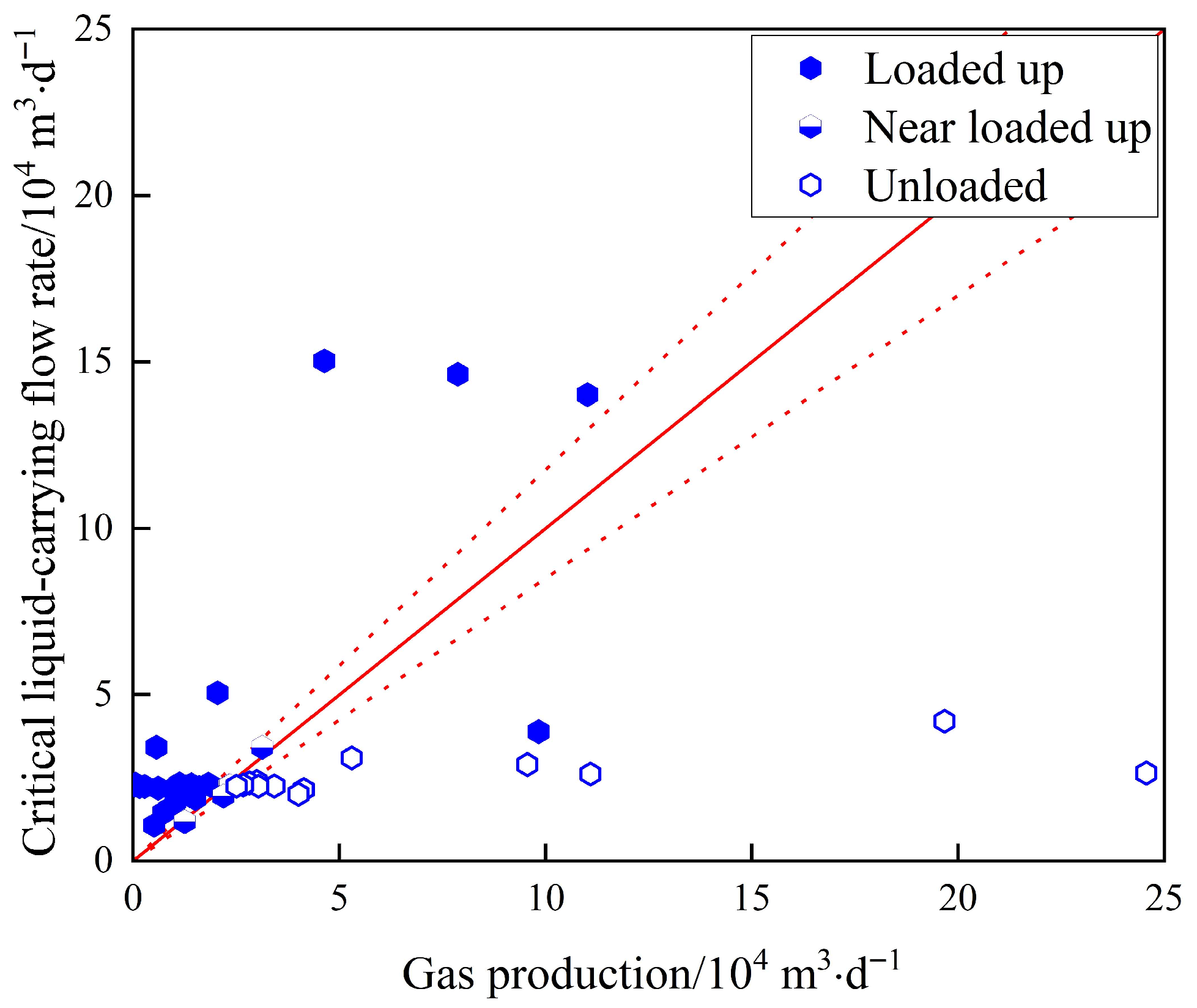
Figure 8, Figure 9, Figure 10, Figure 11 and Figure 12 compare the calculation results of different critical liquid-carrying models with the measured data of gas wells. With the actual gas production rate as the horizontal axis and the model predictions as the vertical axis, a diagonal line is drawn to divide the plot into two regions. If the calculated critical liquid-carrying flow rate for a loaded gas well is above the diagonal line, or if the predicted value for an unloaded gas well is below the diagonal line, the model is considered to have correctly judged the liquid loading status; otherwise, the judgment is considered incorrect. To further analyze gas wells nearing the onset of liquid loading, prediction error lines of ±15% are drawn based on the diagonal line. If the calculated value falls within these error lines, the model prediction is considered accurate; otherwise, the prediction result is considered to have a large error.
As can be seen from Figure 8, Figure 9, Figure 10, Figure 11 and Figure 12, the predictions of the Belfroid model are significantly higher than the actual gas production rates, resulting in misjudgments for 13 wells. The Turner model also yields overestimated predictions, misjudging 11 wells. The Li Min model and the Li Li model misjudge 8 and 7 wells, respectively. In contrast, the proposed model misjudges only one well. For the four wells nearing the onset of liquid loading, the calculation results of the proposed model align better with the actual conditions of the gas wells, with all values falling within the ±15% prediction error range and an average deviation of only 5.9%.

4. Conclusions

(1)
Comprehensively considering the droplet energy losses caused by droplet collision, droplet deformation, and pipe wall friction, and integrating the critical liquid-carrying flow rate prediction models for various well sections with the temperature and pressure field prediction models, a coupled temperature-pressure and liquid-carrying prediction model is established.
(2)
For horizontal gas wells, the vertical section exhibits the lowest critical liquid-carrying flow rate, the inclined section exhibits the highest, and the critical flow rate in the horizontal section lies between those of the vertical and inclined sections.
(3)
Based on the field data analysis of 43 gas wells, the proposed model misjudged only one well. For the four wells approaching liquid loading, the predictions all fell within the ±15% error range, with an average deviation of only 5.9%.

Author Contributions

M.C.: Investigation; Writing—original draft; Formal analysis. J.J.: Writing—review & editing; Visualization; Methodology; Validation. X.X.: Data curation; Validation. Y.Z.: Visualization; Supervision; Investigation. L.Y.: Project administration; Data curation. J.Z. (Corresponding Author): Conceptualization; Funding acquisition; Methodology; Validation. All authors have read and agreed to the published version of the manuscript.

Funding

This research was funded by [1] the Xi’ an Science and Technology Plan Project (24ZDCYISGG0045). [2] State Administration for Market Regulation Science and Technology Plan Project (2024MK0514). [3] Shaanxi Province Technology Innovation Guidance Program (2024QCY-KXJ-019). [4] Xi’an Science and Technology Plan Project (24GXFW0038). [5] Scientific Research Program Funded by Shaanxi Provincial Education Department (24JC053). [6] Shaanxi Province Technology Innovation Guidance Program (2025QCY-KXJ027). [7] Shaanxi Innovation Capability Support Plan—Young Scientists as Rising Stars Program (2025ZC-KJXX-86). [8] Shaanxi Province Market Supervision Technology Plan Project “Key Technology Research and Application of Pipeline External Inspection Robots” (2023KY14). [9] Xi’an Science and Technology Plan Project Key Industrial Chain Technology Research General Project (25ZDLYB00026). [10] Xi’an Science and Technology Plan Project (25ZDLYB00020).

Data Availability Statement

Data is contained within the article.

Conflicts of Interest

All authors declare that there are no other competing interests.

References

  1. Alsanea, M.; Mateus-Rubiano, C.; Karami, H. Liquid loading in natural gas vertical wells: A review and experimental study. SPE Prod. Oper. 2022, 37, 554–571. [Google Scholar] [CrossRef] [Scilit]
  2. Li, J.; Deng, D.; Shen, W.; Gao, Z.; Gong, J. Mechanism of gas well liquid loading and a new model for predicting critical gas velocity. Acta Pet. Sin. 2020, 41, 1266–1277. [Google Scholar] [CrossRef]
  3. Li, L.; Wang, X.; Liu, S.; Liu, J.; Gao, Y.; Li, C. Gas-water flow law in horizontal wellbore and its influencing factors. Acta Pet. Sin. 2019, 40, 1244–1254. [Google Scholar] [CrossRef]
  4. Liu, S.; Yan, X.; Song, Y.; Zhang, H.; Liu, L.; Chen, H. Method for Identifying the Cause of Blowout Stoppage of Horizontal Wells in Constant-Volume Gas Reservoirs and Its Application. Spec. Oil Gas Reserv. 2023, 30, 150–156. [Google Scholar] [CrossRef]
  5. Turner, R.G.; Hubbard, M.G.; Dukler, A.E. Analysis and prediction of minimum flow rate for the continuous removal of liquids from gas wells. J. Pet. Technol. 1969, 21, 1475–1482. [Google Scholar] [CrossRef] [Scilit]
  6. Coleman, S.B.; Clay, H.B.; Mccurdy, D.G.; Norris, L.H. A new look at predicting gas-well load-up. J. Pet. Technol. 1991, 43, 329–333. [Google Scholar] [CrossRef] [Scilit]
  7. Li, M.; Guo, P.; Tan, G. New look on removing liquids from gas wells. Pet. Explor. Dev. 2001, 28, 105–106. [Google Scholar] [CrossRef]
  8. Wang, Y.; Liu, Q. A new method to calculate the minimum critical liquids carrying flow rate for gas wells. Pet. Geol. Oilfield Dev. Daqing 2007, 26, 82–85. [Google Scholar] [CrossRef]
  9. Wang, Z.; Li, Y. The mechanism of continuously removing liquids from gas wells. Acta Pet. Sin. 2012, 33, 681–686. [Google Scholar] [CrossRef]
  10. Li, G.; Yao, Y.; Zhang, R. An improved model for the prediction of liquid loading in gas wells. J. Nat. Gas Sci. Eng. 2016, 32, 198–204. [Google Scholar] [CrossRef] [Scilit]
  11. Belfroid, S.; Schiferli, W.; Alberts, G.; Veeken, C.A.; Biezen, E. Predicting onset and dynamic behaviour of liquid loading gas wells. In Proceedings of the SPE Annual Technical Conference and Exhibition, Denver, CO, USA, 21–24 September 2008. [Google Scholar] [CrossRef] [Scilit]
  12. Li, L.; Zhang, L.; Yang, B.; Yin, Y.; Li, D. Prediction method of critical liquid-carrying flow rate for directional gas wells. Oil Gas Geol. 2012, 33, 650–654. [Google Scholar] [CrossRef]
  13. Ming, R.; He, H.; Hu, Q. A New Model for Continuous Liquid-Carrying Critical Flow Rate of Gas Wells in Turbulence Flow. Bull. Geol. Sci. Technol. 2018, 37, 248–252. [Google Scholar]
  14. Zheng, J.; Li, J.; Dou, Y.; Zhang, Y.; Yang, X.; Zhang, Y. Research progress on the calculation model of critical liquid carrying flow of gas well. Energy Sci. Eng. 2023, 11, 4774–4786. [Google Scholar] [CrossRef] [Scilit]
  15. Richter, H.J. Flooding in tubes and annuli. Int. J. Multiph. Flow 1981, 7, 647–658. [Google Scholar] [CrossRef] [Scilit]
  16. Barnea, D. Transition from annular flow and from dispersed bubble flow-unified models for the whole range of pipe inclinations. Int. J. Multiph. Flow 1986, 12, 733–744. [Google Scholar] [CrossRef] [Scilit]
  17. Luo, S.; Kelkar, M.; Pereyra, E.; Sarica, C. A new comprehensive model for predicting liquid loading in gas wells. SPE Prod. Oper. 2014, 29, 337–349. [Google Scholar] [CrossRef] [Scilit]
  18. Li, J.; Almudairis, F.; Zhang, H. Prediction of critical gas velocity of liquid unloading for entire well deviation. In Proceedings of the International Petroleum Technology Conference, Kuala Lumpur, Malaysia, 10–12 December 2014. [Google Scholar] [CrossRef] [Scilit]
  19. Wang, Z.; Guo, L.; Zhu, S.; Nydal, O.J. Prediction of the critical gas velocity of liquid unloading in a horizontal gas well. SPE J. 2018, 23, 328–345. [Google Scholar] [CrossRef] [Scilit]
  20. Sun, B.; Zhang, Z.; Wang, Z.; Xiang, H. Interfacial friction factor prediction in vertical annular flow based on the interface roughness. Chem. Eng. Technol. 2018, 41, 1833–1841. [Google Scholar] [CrossRef] [Scilit]
  21. Yu, X.; Shi, S.; Li, G.; Fang, J.; Duan, C.; Qi, D. Research on critical liquid loading model for directional wells based on liquid film inversion. Pet. Reserv. Eval. Dev. 2024, 14, 151–158. [Google Scholar] [CrossRef]
  22. Liu, N.; Cao, X.; She, L.; Zhou, M.; Liu, W.; Zhai, X. Method for correcting production data of natural gas wells to improve the accuracy of predicting the critical liquid carrying capacity of the annular mist flow model. Oil Drill. Prod. Technol. 2024, 46, 569–585. [Google Scholar] [CrossRef]
  23. Xie, C.; Qi, Z.; Yan, W.; Huang, X.; Zeng, F. Liquid-carrying mechanism and a new prediction model of downhole-throttling gas wells with water production in tight sandstone gas reservoirs. Nat. Gas Ind. 2025, 45, 105–116. [Google Scholar] [CrossRef]
  24. El Fadili, Y.; Shah, S. A new model for predicting critical gas rate in horizontal and deviated wells. J. Pet. Sci. Eng. 2017, 150, 154–161. [Google Scholar] [CrossRef] [Scilit]
  25. Lin, P.Y.; Hanratty, T.J. Prediction of the initiation of slugs with linear stability theory. Int. J. Multiph. Flow 1986, 12, 79–98. [Google Scholar] [CrossRef] [Scilit]
  26. Andritsos, N.; Hanratty, T.J. Interfacial instabilities for horizontal gas-liquid flows in pipelines. Int. J. Multiph. Flow 1987, 13, 583–603. [Google Scholar] [CrossRef] [Scilit]
  27. Liu, Z.; Reitz, R.D. An analysis of the distortion and breakup mechanisms of high speed liquid drops. Int. J. Multiph. Flow 1997, 23, 631–650. [Google Scholar] [CrossRef] [Scilit]
  28. Helenbrook, B.T.; Edwards, C.F. Quasi-steady deformation and drag of uncontaminated liquid drops. Int. J. Multiph. Flow 2002, 28, 1631–1657. [Google Scholar] [CrossRef] [Scilit]
  29. Azzopardi, B.J.; Piearcey, A.; Jepson, D.M. Drop size measurements for annular two-phase flow in a 20 mm diameter vertical tube. Exp. Fluids 1991, 11, 191–197. [Google Scholar] [CrossRef] [Scilit]
  30. Pan, J.; Wang, W.; Wei, Y.; Chen, J.; Wang, L. A calculation model of critical liquid-carrying velocity of gas wells considering the influence of droplet shapes. Nat. Gas Ind. B 2018, 5, 337–343. [Google Scholar] [CrossRef] [Scilit]
  31. Zheng, J.; Dou, Y.; Cao, Y.; Yan, X. Prediction and analysis of wellbore temperature and pressure of HTHP gas wells considering multifactor coupling. J. Fail. Anal. Prev. 2020, 20, 137–144. [Google Scholar] [CrossRef] [Scilit]
  32. Zheng, J.; Hu, Z.; Xiong, M.; Zhang, Y.; Weng, G.; Yang, Z. Investigation and implementation of temperature field model for high temperature deep well utilizing the element free Galerkin method. J. Energy Resour. Technol. Part B Subsurf. Energy Carbon Capture 2026, 2, 011008. [Google Scholar] [CrossRef] [Scilit]
  33. Du, J.; Jiang, J.; Wang, C. Comparative Study of Carrying Liquid Gas Model and Field Experimental Verification. J. Lanzhou Petrochem. Univ. Vocat. Technol. 2009, 9, 9–12. [Google Scholar] [CrossRef]
  34. Yang, G.; Zou, Y.; Zhou, X.; Fu, C.; Liu, H. Research on the Model of Liquid Carrying Critical Flow Rate of Directional Well. Xinjiang Oil Gas 2012, 8, 76–81. [Google Scholar] [CrossRef]
  35. Ming, R.; He, H.; Hu, Q. A New Predicting Method of the Critical Liquid-Loading Flow Rate for Horizontal Gas Wells. Pet. Geol. Oilfield Dev. Daqing 2018, 37, 81–85. [Google Scholar] [CrossRef]
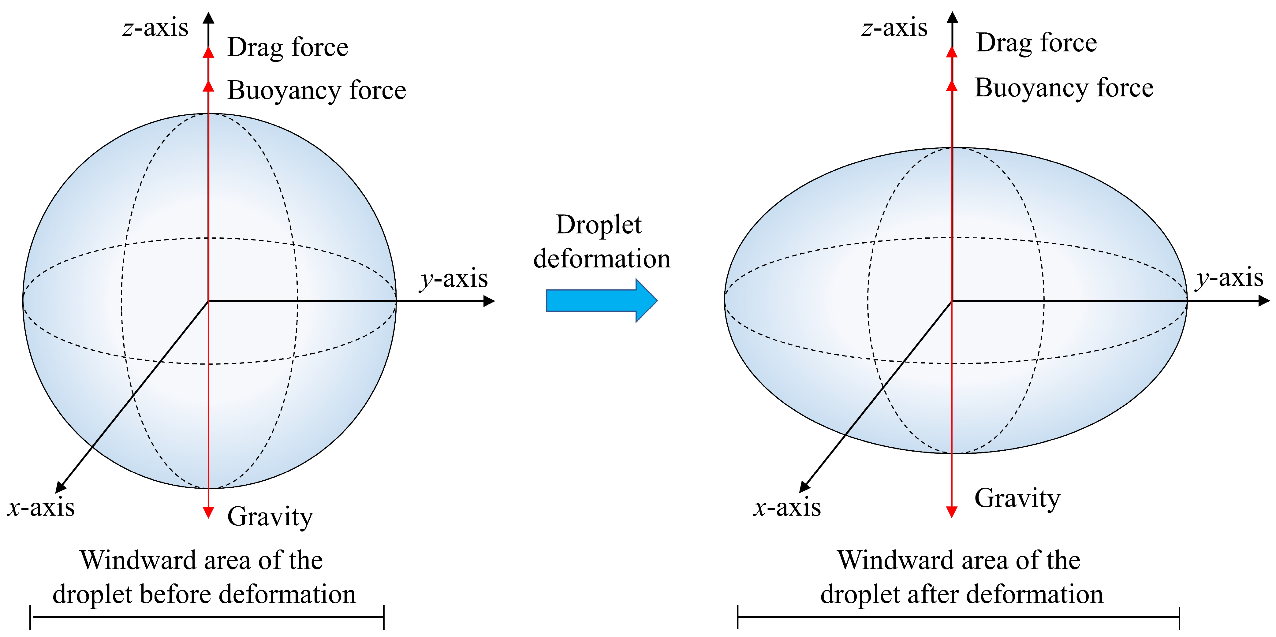
Figure 1. Schematic diagram of droplet deformation and force analysis.
Processes 14 01292 g001
Figure 2. Force analysis of a droplet in an inclined well.
Processes 14 01292 g002
Figure 3. Schematic diagram of the K-H instability effect.
Processes 14 01292 g003
Figure 4. Comparison between calculated and experimental drag coefficients for different models.
Processes 14 01292 g004
Figure 5. Effect of wellhead pressure on the critical liquid-carrying flow rate.
Processes 14 01292 g005
Figure 6. Effect of wellhead temperature on the critical liquid-carrying flow rate.
Processes 14 01292 g006
Figure 7. Effect of tubing inner diameter on the critical liquid-carrying flow rate.
Processes 14 01292 g007
Figure 8. Prediction results of the Turner model.
Processes 14 01292 g008
Figure 9. Prediction results of the Belfroid model.
Processes 14 01292 g009
Figure 10. Prediction results of the Li Min model.
Processes 14 01292 g010
Figure 11. Prediction results of the Li Li model.
Processes 14 01292 g011
Figure 12. Prediction results of the proposed model.
Processes 14 01292 g012
Table 1. Comparison of calculation models for critical liquid-carrying velocity in gas wells.
ModelDrag CoefficientComprehensive CoefficientModel Expression
Turner Model0.446.6 v = 6 . 6 ρ l ρ g σ ρ g 2 0 . 25
Belfroid Model0.446.6 v = 6 . 6 sin 1 . 7 θ 0 . 38 0 . 74 ρ l ρ g σ ρ g 2 0 . 25
Li Min Model1.02.5 v = 2 . 5 ρ l ρ g σ ρ g 2 0 . 25
Li Li ModelDependent on production dataDependent on Wec, k, and Cd v = 5 . 478 λ sin θ + cos θ 0 . 25 ρ l ρ g σ ρ g 2 0 . 25
Proposed ModelDependent on production dataDependent on Wec, k, and CdIterative coupling of the liquid-carrying model with the temperature and pressure model
Table 2. Well production parameters and liquid loading status.
NumberDepth (m)/Inclination Angle (°)Wellhead Pressure (MPa)Tubing ID
(m)
Temperature (K)Gas Production Rate (m3/d)Status
1999.133.160.18760432278,729Loaded Up
2999.132.910.187604322110,164Loaded Up
3999.133.340.18760432246,388Loaded Up
42063.503.100.05067332212,517Near Loaded Up
51951.945.000.06200132221,948Near Loaded Up
62239.0612.650.050673322245,591Unloaded
72239.0619.950.050673322110,929Unloaded
82731.9234.860.05067332295,608Unloaded
93611.8856.640.06200132298,327Loaded Up
103611.8851.060.062001322196,711Unloaded
11/7.200.06023116072Loaded Up
12/7.660.060231123,293Near Loaded Up
13/7.740.060231118,838Loaded Up
14/7.380.060231113,618Loaded Up
15/7.620.060231113,993Loaded Up
16/7.670.060231134,296Unloaded
17/7.840.0602311416Loaded Up
18/8.100.060231111,257Loaded Up
19/7.950.060231114,203Loaded Up
20/7.600.060231130,413Unloaded
21/8.070.060231118,302Loaded Up
22/7.080.06023119551Loaded Up
23/7.860.060231126,711Near Loaded Up
24/7.370.060231116,038Loaded Up
25/7.640.060231123,513Near Loaded Up
26/7.590.060231125,115Near Loaded Up
27/8.080.0602311652Loaded Up
28/7.540.06023111585Loaded Up
29/7.540.060231113,345Loaded Up
30/7.560.06023112868Loaded Up
31371.73//8800Loaded Up
32331.81//5100Loaded Up
333318.1//31,300Loaded Up
34432.59//10,300Loaded Up
35268.3//53,000Unloaded
36276.7//41,400Unloaded
373518//20,500Loaded Up
38243.1230.062/15,130Loaded Up
39302.5510.062/7330Loaded Up
40333.6720.076/28,240Loaded Up
41332.7620.076/40,130Unloaded
4288.98.020.05057/30,100Unloaded
4389.27.280.062/5700Loaded Up
Disclaimer/Publisher’s Note: The statements, opinions and data contained in all publications are solely those of the individual author(s) and contributor(s) and not of MDPI and/or the editor(s). MDPI and/or the editor(s) disclaim responsibility for any injury to people or property resulting from any ideas, methods, instructions or products referred to in the content.