Article

Numerical Simulation of Elastic Waves in VTI Media Using a 17-Point Finite Difference Scheme

1
School of Science, Xuchang University, Xuchang 461000, China
2
College of Geological Engineering & Surveying, Chang’an University, Xi’an 710054, China
*
Author to whom correspondence should be addressed.
Processes 2026, 14(8), 1283; https://doi.org/10.3390/pr14081283
Submission received: 25 February 2026 / Revised: 6 April 2026 / Accepted: 12 April 2026 / Published: 17 April 2026

Abstract

To optimize the stiffness matrix structure for frequency-domain elastic wave forward modeling in 2D VTI (transversely isotropic with a vertical symmetry axis) media—thereby reducing memory consumption and improving computational efficiency—we simplify the conventional 25-point finite-difference scheme to derive a 17-point frequency-domain finite-difference scheme. This approach reformulates the finite-difference operators for the partial derivatives and acceleration terms in the elastic wave equations, reducing the number of grid points involved in the computation by 30 % compared to the 25-point scheme. The optimized matrix construction leverages sparse matrix storage techniques, decreasing memory usage by approximately 27 % . Numerical validation, conducted using a double-layer VTI medium model and the Marmousi model with three major faults and an anticline containing limestone layers at the base of the faults, demonstrates that the 17-point finite-difference scheme maintains comparable accuracy while requiring 14 % less computation time and featuring a 25 % reduction in nonzero elements within the impedance matrix. Comparisons of wavefield snapshots and receiver components (horizontal component U and vertical component V) support this conclusion. These improvements enable the use of more efficient iterative solvers.

1. Introduction

Seismic anisotropy, characterized by directionally dependent wave propagation velocities, is ubiquitous in the Earth’s subsurface. Notable examples include the passive margin systems of offshore West Africa, the salt-dominated Gulf of Mexico Basin, and gas-hydrate-bearing sediments in the South China Sea Basin, where layered anisotropic stratigraphy is prevalent. Among the various anisotropic symmetries, transverse isotropy (TI)—which features a single symmetry axis—represents the most geologically common configuration.
Frequency-domain forward modeling was first proposed by Lysmer and Drake, who investigated wave propagation characteristics in various media using this scheme [1]. Thomsen laid the parametric foundation for all subsequent numerical simulations in VTI media [2]. Pratt extended the finite-difference forward modeling scheme to frequency-domain inversion in 1990 [3,4]. Alkhalifah and Tsvankin introduced anisotropic parameters and laid the foundation for the pseudo-acoustic approximation in VTI media, which has been widely applied to qP-wave simulation in finite-difference (FD) methods [5]. Jo et al. introduced an optimized 9-point difference operator and successfully implemented this approach in frequency-domain acoustic wave equation simulations in 1996 [6]. Building upon Jo’s work, Stekl and Pratt incorporated the optimized 9-point finite difference scheme into elastic wave equations for viscoelastic media [7]. In 1998, Shin et al. proposed a 25-point finite-difference scheme for the frequency-domain acoustic wave equation, which reduced numerical dispersion requirements but increased the bandwidth of the impedance matrix [8]. Pratt argued that seismic waveform inversion in the frequency domain does not require full-frequency computations; instead, partial frequency components suffice to invert model parameters, drastically reducing computational load [9]. Min proposed a 25-point finite difference scheme that minimized numerical dispersion through optimized coefficients while reducing spatial sampling points [10]. Sirgue and Pratt demonstrated that inversion imaging can be achieved using sparse frequency components. This technique markedly enhanced the computational efficiency of frequency-domain waveform inversion. They also emphasized that strategic frequency selection could yield results comparable to time-domain inversion [11]. Wu et al. implemented the 25-point scheme in forward modeling for both VTI and TTI media [12,13]. Operto et al. developed a 2D finite-difference, frequency-domain scheme for modeling viscoacoustic seismic waves in transversely isotropic media with a tilted symmetry axis [14]. Kostin, V. I. et al. present a finite-difference method for the numerical simulation of seismic wave propagation through multiscale media, aiming to improve computational accuracy and efficiency in complex geological structures [15]. Lisitsa et al. directly embedded Thomsen parameters into high-order staggered-grid FD stencils and established the corresponding stability criterion for VTI media [16]. Gu and colleagues developed a 21-point finite-difference scheme for numerical simulation of 2D elastic waves, demonstrating comparable accuracy to the 25-point finite-difference scheme while reducing computational memory and time by 15% [17]. Pevzner, R. et al. detailed the implementation procedures of the rotated staggered grid (RSG) in VTI media and analyzed the stability of free-surface boundary handling [18]. Benjamin et al. evaluated weighted-averaged 27-point finite-difference operators for 3D viscoelastic wave modeling in the frequency domain [19]. Fomel, S. et al. introduced a lowrank symbol approximation method to efficiently and accurately approximate seismic wave extrapolation operators, enabling fast simulation of wave propagation in heterogeneous anisotropic media [20]. Lipnikov et al. presented the first comprehensive review of the 50-year history of mimetic methodology and provided sufficient details to construct various discrete operators on unstructured polygonal and polyhedral meshes, summarizing the major convergence results for mimetic approximations [21]. Ping et al. systematically implemented the spectral element method for seismic wave forward modeling in viscoelastic VTI media, filling the gap in the application of the spectral element method to anisotropic and viscoelastic composite media [22]. Reshetova et al. demonstrated the specific parallel strategies and memory optimization techniques for VTI elastic wave modeling on graphics processing units (GPUs) Pevzner et al. proposed optimized finite-difference coefficients tailored for VTI media, reducing the dispersion error by approximately 40% under the same grid resolutionTcheverda and Kostin revealed that conventional FD schemes may generate spurious growing modes and proposed constrained modified difference coefficients to suppress this instability [23]. Boada et al. introduced 2nd- and 4th-order mimetic formulations for computing anisotropic fluxes for anisotropic elliptic equations [24]. Sethi et al. developed a 3D mimetic finite difference (MFD) algorithm based on CUDA for arbitrarily anisotropic media, employing a fully staggered-grid strategy [25]. Dong et al. leveraged the affine transformation to develop an affine 25-point finite-difference scheme that boasts higher accuracy [26]. Shin first introduced tensor-train (TT) decomposition into elastic wavefield decomposition in VTI media and established a TT decomposition-based framework for elastic wavefield separation in VTI media [27]. Many further studies have shown that finite difference forward simulation can further reduce memory consumption and computation time.
The advantages of frequency-domain forward modeling arise from discretizing the frequency-domain elastic wave equations using finite-difference operators, which circumvents the accumulation of temporal errors. By processing independent frequency components, this approach allows flexible selection of frequency bands and is inherently well-suited for parallel computing. However, its rapid advancement is hindered by two key challenges: the need to determine optimal spatial sampling parameters before simulation, and the computational burden associated with solving large sparse matrix equations during forward modeling.
This computational burden becomes particularly pronounced in geophysical inversion, where forward modeling must be performed repeatedly. Variations in memory usage and computational cost across successive simulations can significantly impact the overall inversion process. A notable issue arises with the 25-point finite-difference scheme commonly used in frequency-domain methods: the resulting sparse matrix exhibits a substantially larger bandwidth than that of the 9-point scheme, with approximately 25 nonzero entries per row, leading to reduced sparsity and increased memory demands for direct solvers. For three-dimensional problems, extending this approach to its 125-point counterpart leads to a drastic increase in matrix bandwidth. Consequently, reducing the number of grid points required in the simulation—while maintaining accuracy—has become a key research direction aimed at lowering memory requirements and improving computational efficiency.
As an improvement, we propose a 17-point finite-difference scheme for elastic wave frequency-domain forward modeling based on the conventional 25-point scheme. Numerical validation demonstrates that, compared to the 25-point scheme, the 17-point variant imposes slightly stricter grid spacing requirements while offering comparable computational accuracy, reduced computation time, and a narrower impedance matrix bandwidth.

2. A 17-Point Finite-Difference Scheme

The frequency-domain wave equations for a 2D VTI medium are as follows:
C 11 2 U x 2 + C 44 2 U z 2 + ( C 13 + C 44 ) 2 V x z = ρ ω 2 U , C 44 2 V x 2 + C 33 2 V z 2 + ( C 13 + C 44 ) 2 U x z = ρ ω 2 V .
where U represents horizontal displacement, V represents vertical displacement, C 11 = ρ v p 2 ( 1 + 2 ε ) , C 33 = ρ v p 2 , C 44 = ρ v s 2 , C 13 = ρ ( v p 2 v s 2 ) ( ( 1 + 2 δ ) v p 2 v s 2 ) ρ v s 2 , ρ ( x , z ) represents the medium density, ε and δ are the VTI medium anisotropy factors, and ω is the angular frequency.
In Equation (1), there are two acceleration terms and six partial derivative terms. Figure 1 shows the point distribution required to discretize these terms using the 17-point finite-difference scheme. The coefficients a 1 to a 12 correspond to the weighting coefficients for grid points at various distances from the central point in the finite-difference stencil.
Mathematically, the 17-point finite-difference scheme can be interpreted as retaining only the grid points along the horizontal, vertical, and 45° diagonal directions from the original 25-point scheme, while omitting the grid points along the 135° diagonal and other secondary directions. This configuration maintains comparable accuracy in wave propagation simulation while reducing the number of grid points by eight, thereby significantly reducing memory requirements and improving both computational efficiency and stability in subsequent calculations.
For the acceleration term ρ ω 2 U , the wavefield values at all grid points are weighted and averaged, with grid points at the same distance from the calculation point sharing the same weighting coefficient. The distribution of the weighting coefficients is shown in Figure 1a. The coefficients a 1 to a 5 correspond to the weighting coefficients for grid points at various distances from the central point in the finite-difference stencil. The expression is as follows:
ρ ω 2 U = ρ ω 2 a 1 U i , j + ρ ω 2 a 2 ( U i , j + 1 + U i + 1 , j + U i 1 , j + U i , j 1 ) + ρ ω 2 a 3 ( U i + 1 , j + 1 + U i + 1 , j 1 + U i 1 , j + 1 + U i 1 , j + 1 ) + ρ ω 2 a 4 ( U i , j + 2 + U i , j 2 + U i 2 , j + U i + 2 , j ) + ρ ω 2 a 5 ( U i + 2 , j + 2 + U i + 2 , j 2 + U i 2 , j + 2 + U i 2 , j + 2 ) .
For the partial derivative term 2 U x 2 , the distribution of weighting coefficients is shown in Figure 1b. Two central difference operators are constructed along the row coinciding with the x-axis in the figure, with weighting coefficients a 9 and a 10 . For the remaining rows, only one central difference operator is used per row, with a weighting coefficient of either a 9 or a 10 . These five difference operators are then combined using weighting coefficients a 6 , a 7 , and a 8 . The resulting expression is:
2 U x 2 = a 6 x 2 a 9 ( U i + 1 , j 2 U i , j + U i 1 , j ) + a 10 ( U i + 2 , j 2 U i , j + U i 2 , j ) + a 7 x 2 a 9 ( U i + 1 , j + 1 2 U i , j + 1 + U i 1 , j + 1 ) + a 9 ( U i + 1 , j 1 2 U i , j 1 + U i 1 , j 1 ) + a 8 x 2 a 10 ( U i + 2 , j + 2 2 U i , j + 2 + U i 2 , j + 2 ) + a 10 ( U i + 2 , j 2 2 U i , j 2 + U i 2 , j 2 ) .
For the partial derivative term 2 U z 2 , the distribution of weighting coefficients is shown in Figure 1c. Along the row corresponding to the z-axis in the figure, two central difference operators are constructed with weighting coefficients a 9 and a 10 . For the remaining rows, only one central difference operator is used per row, with a weighting coefficient of either a 9 or a 10 . These five difference operators are then combined via a weighted average using coefficients a 6 , a 7 , and a 8 . The resulting expression is:
2 U z 2 = a 6 z 2 a 9 ( U i , j + 1 2 U i , j + U i , j 1 ) + a 10 ( U i , j + 2 2 U i , j + U i , j 2 ) + a 7 z 2 a 9 ( U i + 1 , j + 1 2 U i + 1 , j + U i + 1 , j 1 ) + a 9 ( U i 1 , j + 1 2 U i 1 , j + U i 1 , j 1 ) + a 8 z 2 a 10 ( U i + 2 , j + 2 2 U i + 2 , j + U i + 2 , j 2 ) + a 10 ( U i 2 , j + 2 2 U i 2 , j + U i 2 , j 2 ) .
For the mixed partial derivative term 2 U x z , the distribution of weighting coefficients a 11 and a 12 is shown in Figure 1d. The resulting expression is:
2 U x z = a 11 4 x z ( U i + 1 , j + 1 U i + 1 , j 1 U i 1 , j + 1 + U i 1 , j 1 ) + a 12 16 x z ( U i + 2 , j + 2 U i + 2 , j 2 U i 2 , j + 2 + U i 2 , j 2 ) .
Similarly, difference operators for the remaining terms can be constructed. After substituting these operators into Equation (1) and performing appropriate algebraic manipulations, the discrete form is obtained as follows:
C 1 , 1 U i , j + C 1 , 2 U i , j + 1 + C 1 , 2 U i , j 1 + C 1 , 3 U i + 1 , j + C 1 , 3 U i 1 , j + C 1 , 4 U i + 1 , j + 1 + C 1 , 4 U i + 1 , j 1 + C 1 , 4 U i 1 , j + 1 + C 1 , 4 U i 1 , j 1 + C 1 , 5 U i , j + 2 + C 1 , 5 U i , j 2 + C 1 , 6 U i + 2 , j + C 1 , 6 U i 2 , j + C 1 , 7 U i + 2 , j + 2 + C 1 , 7 U i + 2 , j 2 + C 1 , 7 U i 2 , j + 2 + C 1 , 7 U i 2 , j 2 + C k , 1 ( V i + 1 , j + 1 V i + 1 , j 1 V i 1 , j + 1 + V i 1 , j 1 ) + C k , 2 ( V i + 2 , j + 2 V i + 2 , j 2 V i 2 , j + 2 + V i 2 , j 2 ) = 0 ,
C 2 , 1 V i , j + C 2 , 2 V i , j + 1 + C 2 , 2 V i , j 1 + C 2 , 3 V i + 1 , j + C 2 , 3 V i 1 , j + C 2 , 4 V i + 1 , j + 1 + C 2 , 4 V i + 1 , j 1 + C 2 , 4 V i 1 , j + 1 + C 2 , 4 V i 1 , j 1 + C 2 , 5 V i , j + 2 + C 2 , 5 V i , j 2 + C 2 , 6 V i + 2 , j + C 2 , 6 V i 2 , j + C 2 , 7 V i + 2 , j + 2 + C 2 , 7 V i + 2 , j 2 + C 2 , 7 V i 2 , j + 2 + C 2 , 7 V i 2 , j 2 + C k , 1 ( U i + 1 , j + 1 U i + 1 , j 1 U i 1 , j + 1 + U i 1 , j 1 ) + C k , 2 ( U i + 2 , j + 2 U i + 2 , j 2 U i 2 , j + 2 + U i 2 , j 2 ) = 0 .
The coefficients are represented as follows:
C 1 , 1 = ( 2 a 6 a 9 x 2 + 2 a 6 a 10 4 x 2 ) C 11 + ( 2 a 6 a 9 z 2 + 2 a 6 a 10 4 z 2 ) C 44 a 1 ω 2 , C 1 , 2 = a 6 a 9 x 2 C 11 2 a 7 a 9 z 2 C 44 + a 2 ω 2 , C 1 , 3 = a 6 a 9 x 2 C 44 2 a 7 a 9 z 2 C 11 + a 2 ω 2 , C 1 , 4 = a 6 a 9 x 2 C 11 + 2 a 7 a 9 z 2 C 44 + a 3 ω 2 , C 1 , 5 = a 6 a 10 4 x 2 C 11 2 a 8 a 10 4 z 2 C 44 + a 4 ω 2 , C 1 , 6 = a 6 a 10 4 x 2 C 44 2 a 8 a 10 4 z 2 C 11 + a 4 ω 2 , C 1 , 7 = a 8 a 10 4 x 2 C 11 + a 8 a 10 4 z 2 C 44 + a 5 ω 2 , C 2 , 1 = ( 2 a 6 a 9 x 2 + 2 a 6 a 10 4 x 2 ) C 44 + ( 2 a 6 a 9 z 2 + 2 a 6 a 10 4 z 2 ) C 33 a 1 ω 2 , C 2 , 2 = a 6 a 9 x 2 C 44 2 a 7 a 9 z 2 C 33 + a 2 ω 2 , C 2 , 3 = a 6 a 9 x 2 C 33 2 a 7 a 9 z 2 C 44 + a 2 ω 2 , C 2 , 4 = a 6 a 9 x 2 C 44 + 2 a 7 a 9 z 2 C 33 + a 3 ω 2 , C 2 , 5 = a 6 a 10 4 x 2 C 44 2 a 8 a 10 4 z 2 C 33 + a 4 ω 2 , C 2 , 6 = a 6 a 10 4 x 2 C 33 2 a 8 a 10 4 z 2 C 44 + a 4 ω 2 , C 2 , 7 = a 8 a 10 4 x 2 C 44 + a 8 a 10 4 z 2 C 33 + a 5 ω 2 , C k , 1 = a 11 ( C 13 + C 44 ) 4 x z , C k , 2 = a 12 ( C 13 + C 44 ) 16 x z .
Equation (6) represents the discrete formula at grid point ( i , j ) in the model. For each coordinate point in the model, an equation is established. These equations, combined with the seismic source term, yield the following matrix equation:
A ( v , ω ) Y ( ω ) = F ( ω ) ,
For each frequency, let the number of grid points in the computational domain be N z × N x , denoted as N = N z × N x . Then, A is a 2 N × 2 N impedance matrix, Y is the 2 N × 1 unknown wavefield vector (comprising U and V), and F is a 2 N × 1 source term vector.

3. Dispersion Analysis and Weighting Coefficients

Based on the dispersion analysis of the 25-point finite-difference scheme by Min et al. [10] and Equation (1), the dispersion relation for phase velocity of the 17-point finite-difference scheme in VTI media can be expressed as follows:
V p p h V p = 1 2 π 1 G s 1 2 A ( B + C ) , V s p h V s = 1 2 π 1 G s 1 2 A ( B C ) .
where
A = P m , B = C 11 P x x + C 44 P z z + C 44 P x x + C 33 P z z , C = B 2 4 ( ( C 11 P x x + C 44 P z z ) ( C 44 P x x + C 33 P z z ) ( C 13 + C 44 ) 2 P x z 2 ) ,
and
P m = a 1 + 2 a 2 ( cos ( k x ) + cos ( k z ) ) + 4 a 3 cos ( k x ) cos ( k z ) + 2 a 4 ( cos ( 2 k x ) + cos ( 2 k z ) ) + 4 a 5 cos ( 2 k x ) cos ( 2 k z ) , P x x = a 6 ( 4 a 9 sin 2 ( k x 2 ) + a 10 sin 2 ( k x ) ) 8 a 7 a 9 cos ( k z ) sin 2 ( k x 2 ) 2 a 8 a 10 cos ( 2 k z ) sin 2 ( k x ) , P z z = a 6 ( 4 a 9 sin 2 ( k z 2 ) + a 10 sin 2 ( k z ) ) 8 a 7 a 9 cos ( k x ) sin 2 ( k z 2 ) 2 a 8 a 10 cos ( 2 k x ) sin 2 ( k z ) , P x z = a 11 sin ( k x ) sin ( k z ) a 12 4 sin ( 2 k x ) sin ( 2 k z ) .
where V p is the compressional wave velocity, V s is the shear wave velocity, V p p h and V s p h are the phase velocities of the compressional and shear waves, respectively, G s is the number of grid points per shear wavelength, = x = z is the grid spacing, and the wavenumbers k x and k z are functions of the propagation angle θ measured from the x-axis. Additionally, a 1 through a 12 are weighting coefficients.
To calculate the weighting coefficients a 1 to a 12 , let K = 1 / G s . The objective function can be
E ( a 1 a 12 ) = 1 V p h ( K , θ , σ , a 1 a 12 ) V 2 d K d θ .
Taking into account factors such as the reciprocal of the number of grid points per shear wavelength K, the wave propagation angle θ , and Poisson’s ratio σ = λ 2 ( λ + μ ) , we obtain the weighting coefficients for the 17-point finite-difference scheme using the Nelder–Mead simplex method. The resulting coefficients are shown in Table 1.
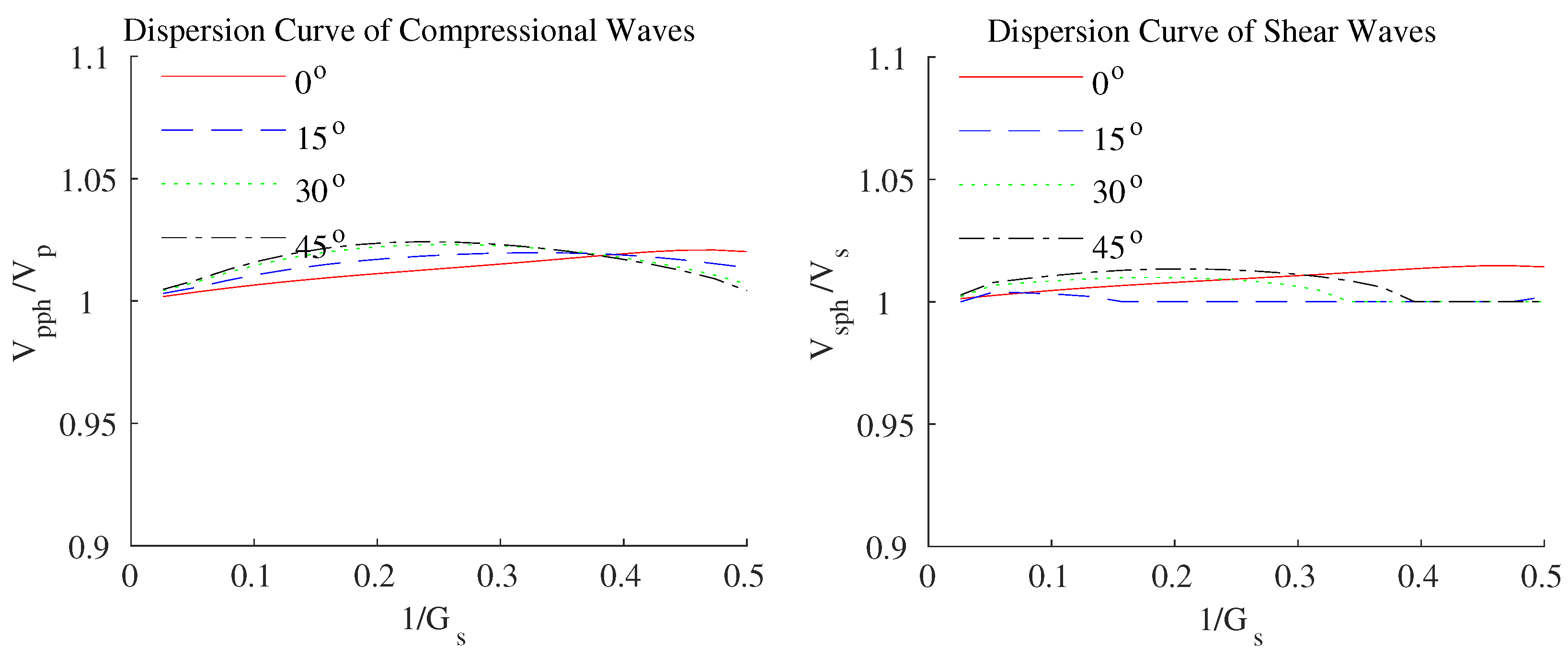
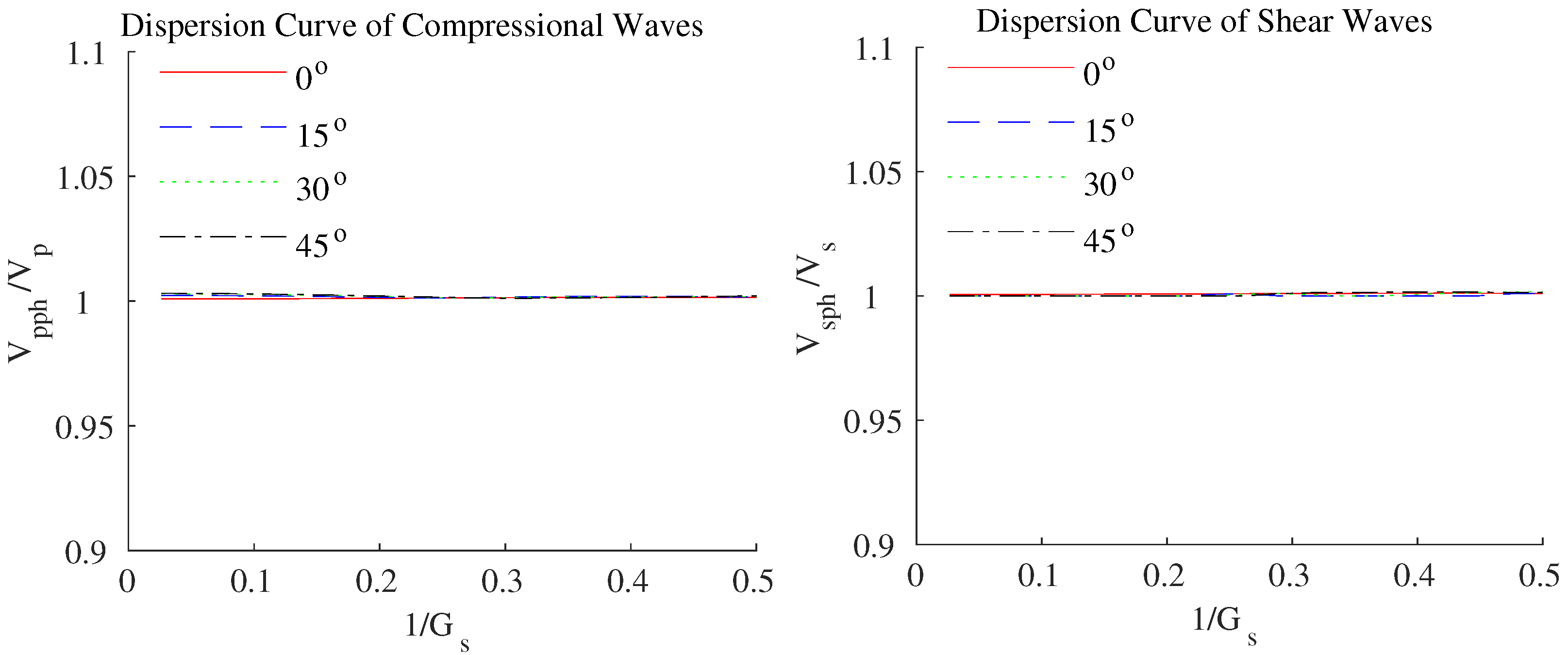
Using the coefficients in Table 1 and the phase velocity dispersion Equation (8), dispersion curves are generated for varying grid sizes, propagation angles, and Poisson’s ratios. Specifically, Figure 2 presents the results for a Poisson’s ratio of 0.25 using the 17-point finite-difference scheme, while Figure 3 shows the corresponding curves for the same Poisson’s ratio using the 25-point scheme.

Stability Condition Analysis

In frequency-domain numerical simulations, there is no time marching; therefore, the CFL condition is not involved. When applying the 17-point finite-difference scheme, the wavelength sampling criterion must be satisfied; otherwise, numerical dispersion will blow up at high wavenumbers, manifesting as numerical instability. Intuitively, the grid spacing should satisfy the following condition:
x , z λ min N .
where x and z denote the grid spacing, λ min represents the minimum wavelength, and N stands for the number of grid points per wavelength. To keep phase velocity errors within 1%, the 17-point finite-difference scheme requires at least 8.7 grid points per wavelength, whereas the 25-point scheme requires at least 3.3 grid points. Although the 17-point scheme imposes a slightly stricter requirement on grid density, the conventional grid discretization generally remains sufficient for most applications.

4. Results

4.1. Numerical Simulation of Simple VTI Medium Model

The VTI medium model parameters are as follows: P-wave velocity V p = 3000 m/s, S-wave velocity V s = 2000 m/s, density ρ = 2500 kg/m3, and anisotropy factors ε = 0.5 and δ = 0.1 . The spatial grid consists of N x = N z = 160 grid points with a uniform spacing of x = z = 5 m. A perfectly matched layer (PML) boundary condition with a thickness of 20 grid points is applied. The recording time is 0.25 s; in the frequency domain, this corresponds to 19 frequency points processed separately. The seismic source is a Ricker wavelet with a dominant frequency of 25 Hz, located at grid coordinates (80, 80), while the receiver is positioned at (100, 100). All numerical simulations were performed on a platform equipped with an Intel Core i5-10400 processor and 16 GB of dual-channel DDR4-3200 MHz memory.
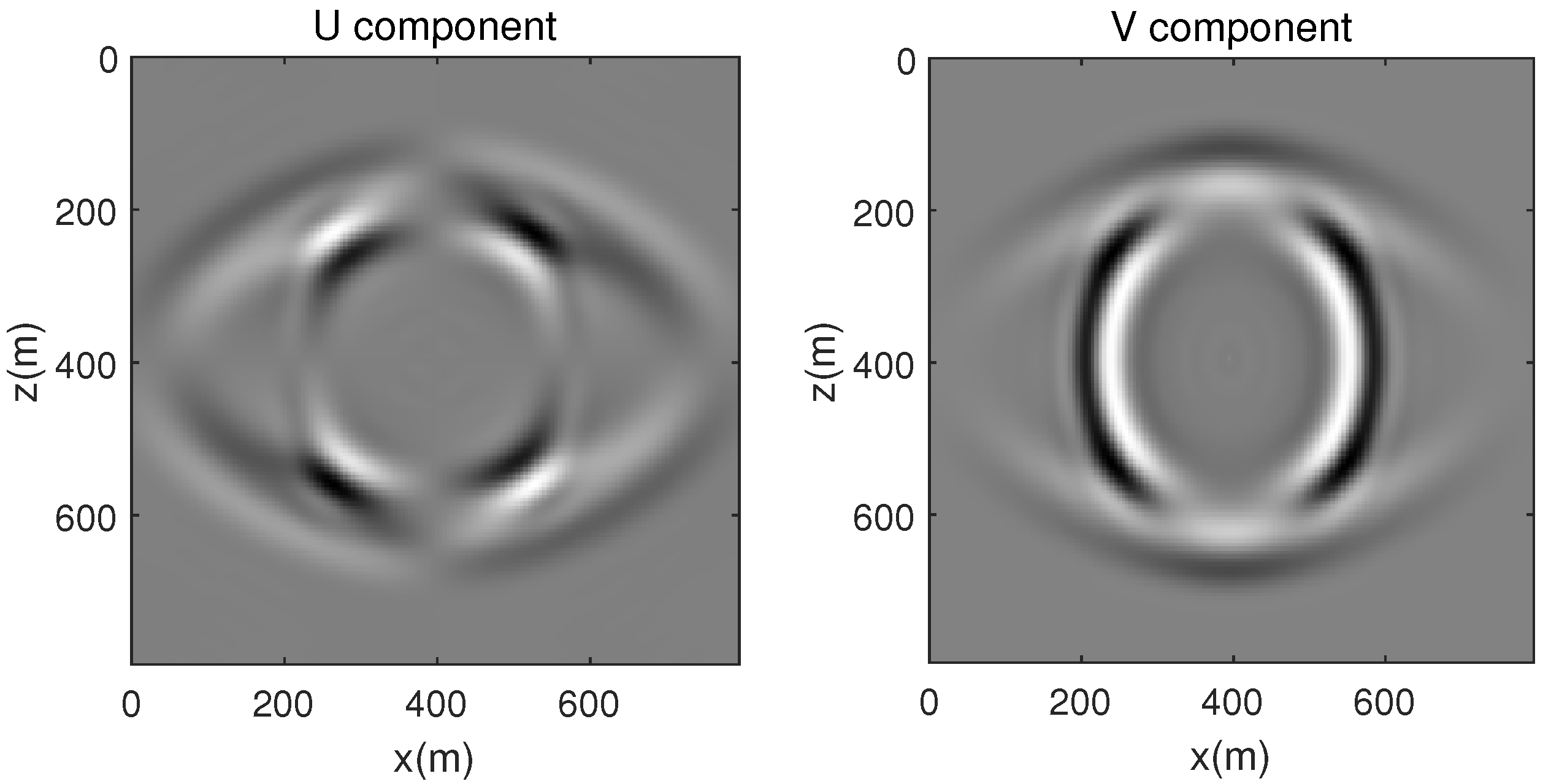
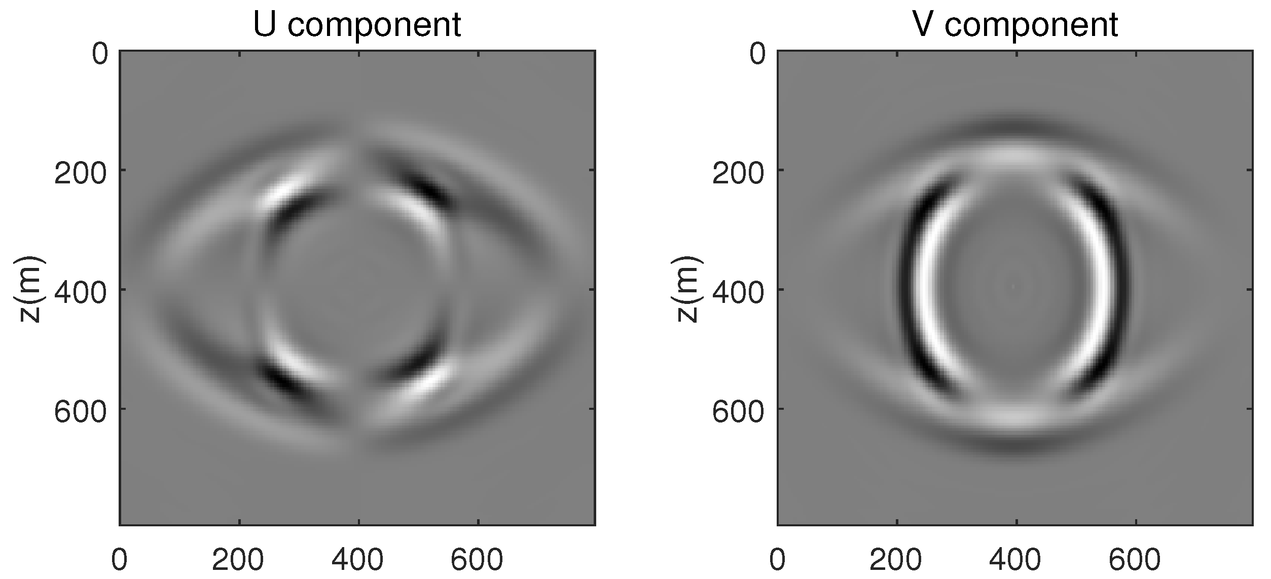
Figure 4 and Figure 5 show the wavefield snapshots of the 17-point and 25-point finite-difference schemes at 125 ms. The two snapshots are nearly identical. The wavefronts of the excited P-waves are no longer circular but instead appear elliptical or diamond-shaped, demonstrating that the propagation velocity of elastic waves in anisotropic media is direction-dependent. In such media, P-waves and S-waves are inherently coupled; consequently, even when a P-wave source is excited in a homogeneous medium, S-waves are generated. The resulting S-wave wavefronts exhibit complex geometries, including triplication caused by directional velocity variations and shear-wave splitting.
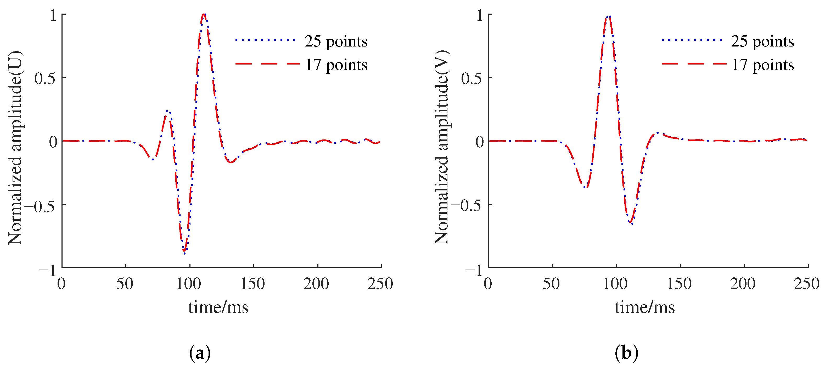
For further comparative analysis, the U and V components of the 17-point and 25-point finite-difference schemes at the receiver are plotted. Both components exhibit strong correspondence, with only minor discrepancies observed near the extremum in Figure 6.

4.2. Impedance Matrix

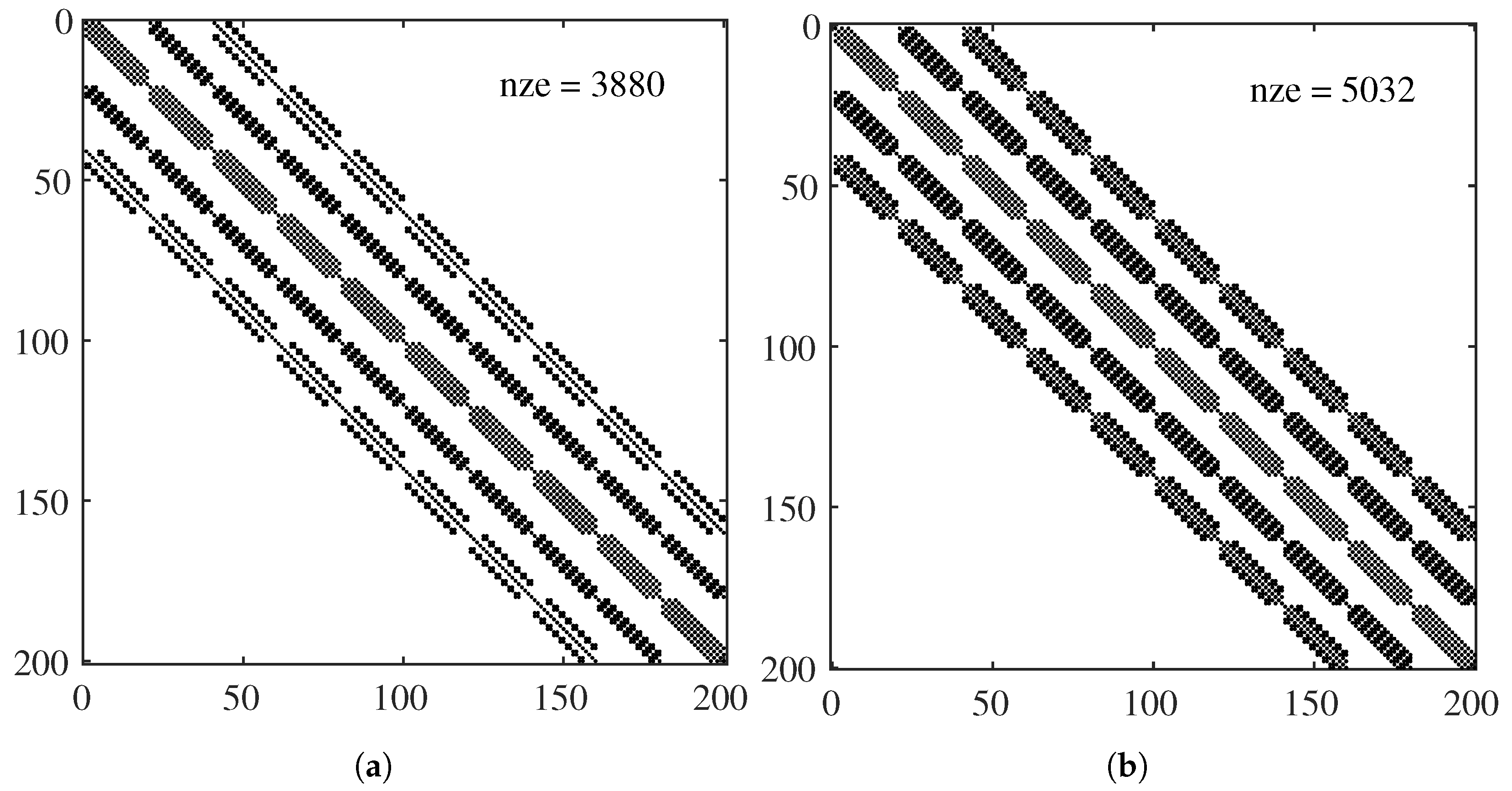
To visually compare the impedance matrices of the two finite-difference schemes, we consider a computational domain with a grid of 10 × 10 points, resulting in an impedance matrix of size 200 × 200 . Figure 7 illustrates the distribution of nonzero elements in the impedance matrices for the 17-point and 25-point finite-difference schemes. The number of nonzero elements is n z e 17 = 3880 for the 17-point scheme and n z e 25 = 5032 for the 25-point scheme.
When the computational domain has a grid of 160 × 160 points, the actual computational area expands to 200 × 200 after adding a 20-grid PML boundary on each side. The impedance matrix correspondingly increases to 80 , 000 × 80 , 000 , with n z e 17 = 1 , 976 , 080 and n z e 25 = 2 , 606 , 512 . The nonzero element ratios are 0.03 % for the 17-point scheme and 0.04 % for the 25-point scheme. Equation system (7) thus becomes a large-scale system that is difficult to store and solve using conventional methods, making sparse matrix storage and computation necessary.
After adopting sparse format storage, the impedance matrix size per frequency point is 5.57 MB for the 17-point scheme and 7.32 MB for the 25-point scheme, representing a reduction of 23.91 % . The average solution time for Equation (7) is 6.3233 s for the 17-point scheme and 7.3156 s for the 25-point scheme, representing a reduction of 14.56 % . During program execution, the memory consumption is 3447.36 MB for the 17-point scheme and 4538.83 MB for the 25-point scheme, reflecting a 24.05 % reduction attributable to the simplified finite-difference scheme. A detailed comparison is shown in Table 2.
Although the differences in time and memory consumption per individual forward simulation may appear negligible, the cumulative reductions are substantial in inversion processes that require thousands of such simulations.

4.3. Numerical Simulation of Double-Layer VTI Medium Model

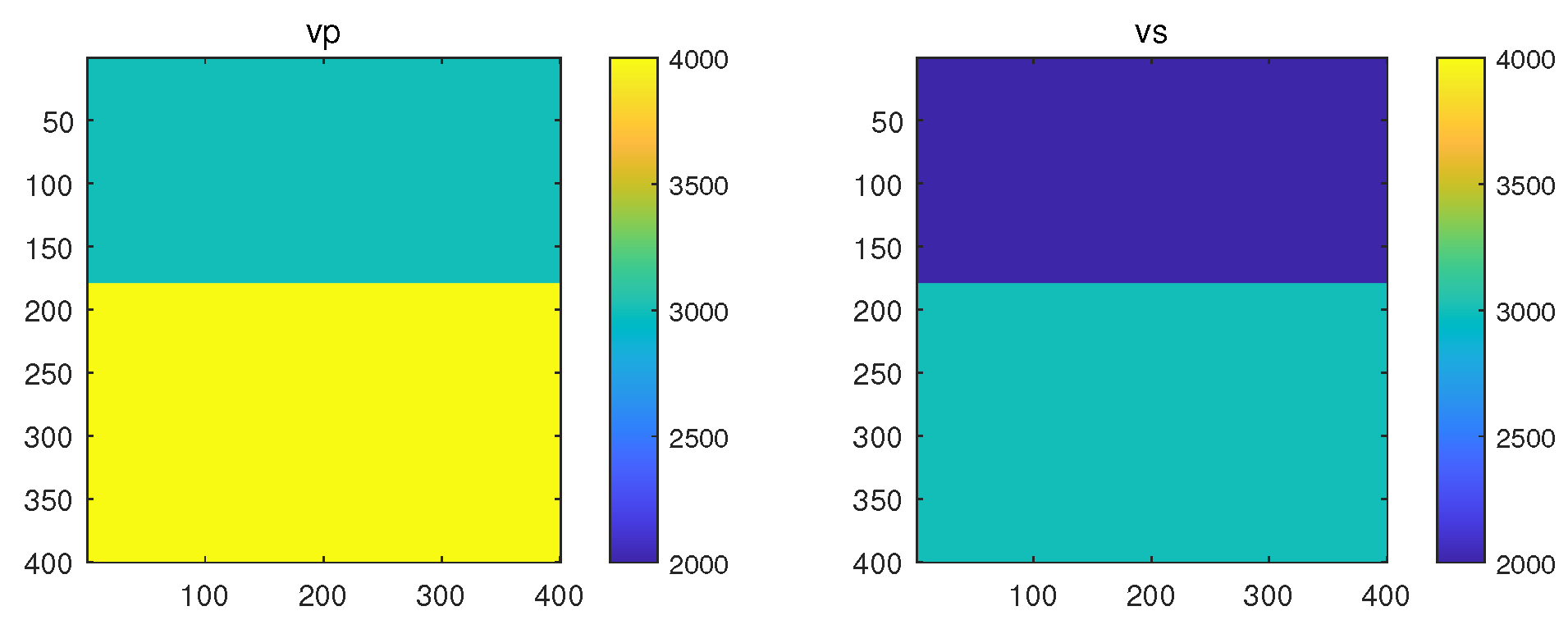
To further validate the proposed forward modeling scheme, a two-layer VTI medium model is designed, as shown in Figure 8.
The model parameters are listed in Table 3. The spatial grid consists of N x = N z = 360 grid points with a uniform spacing of x = z = 4 m, and a Ricker wavelet with a dominant frequency of 20 Hz is located at grid coordinates (120, 180). A perfectly matched layer (PML) with a thickness of 20 grid points is applied on each side, resulting in an actual computational domain size of 400 × 400 .
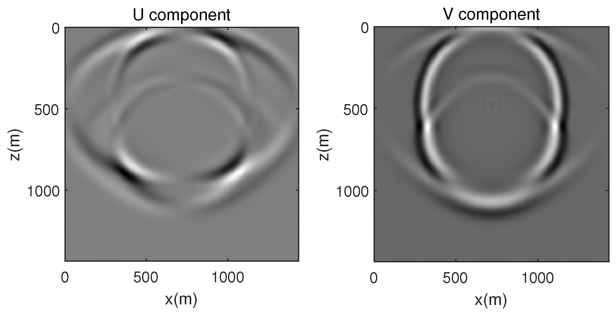
The horizontal and vertical component snapshots at 225 ms are displayed in Figure 9. The snapshots capture the characteristics of the two-layer model. The reflected and transmitted waves at the interface are distinctly visible, and the converted waves are also prominent. These modeling outcomes indicate that the 17-point finite-difference scheme is effective for numerical simulations of typical models.

4.4. Partion of Marmousi Model

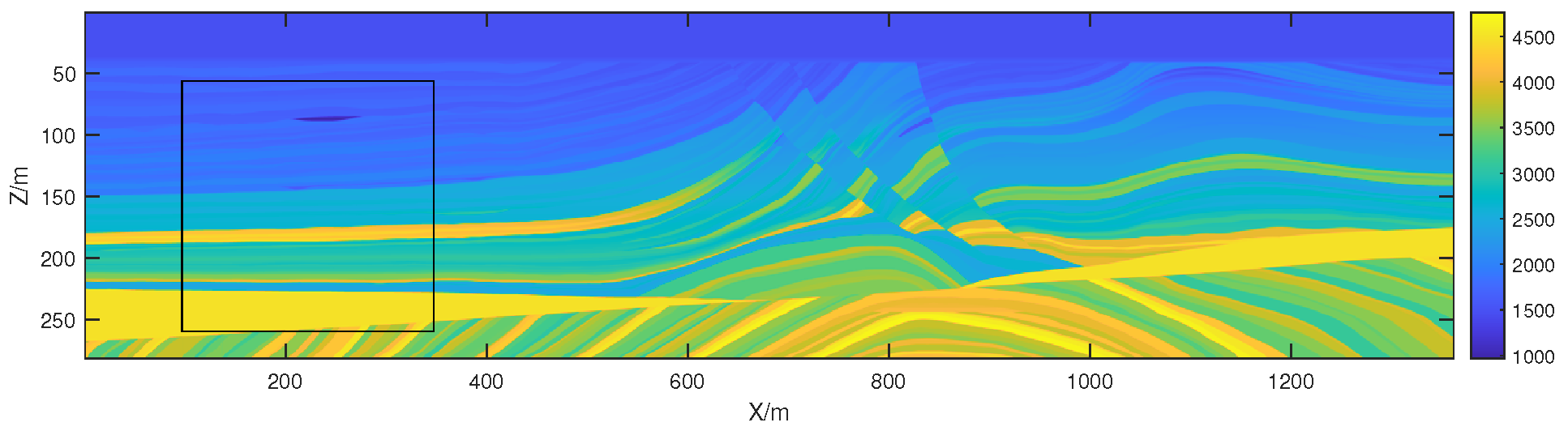
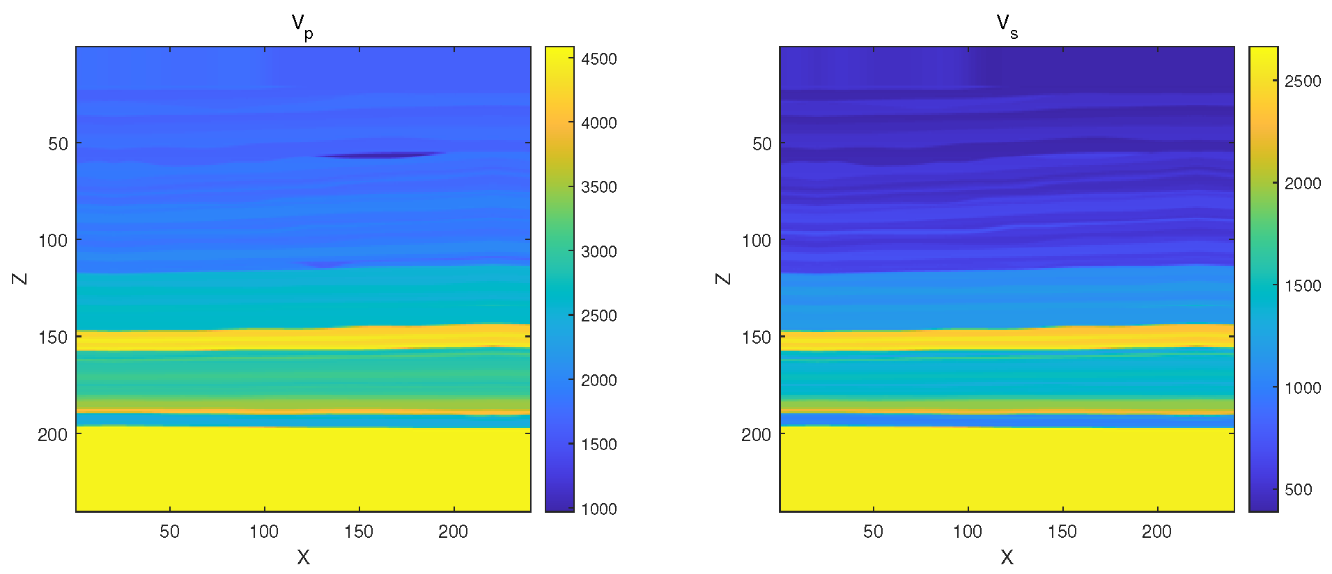
The Marmousi model was originally designed by the Institut Français du Pétrole (IFP). In 2006, Martin et al. [28] extended it to an elastic wave model. This model contains three major faults, with an anticline containing limestone layers at the base of the faults. High-velocity salt domes flank the deep layers on both sides, and the lowermost section features an anticline hosting a hydrocarbon reservoir. Owing to the large size of the original model, we compressed it and extracted a portion for numerical simulation, as shown in Figure 10 and Figure 11.
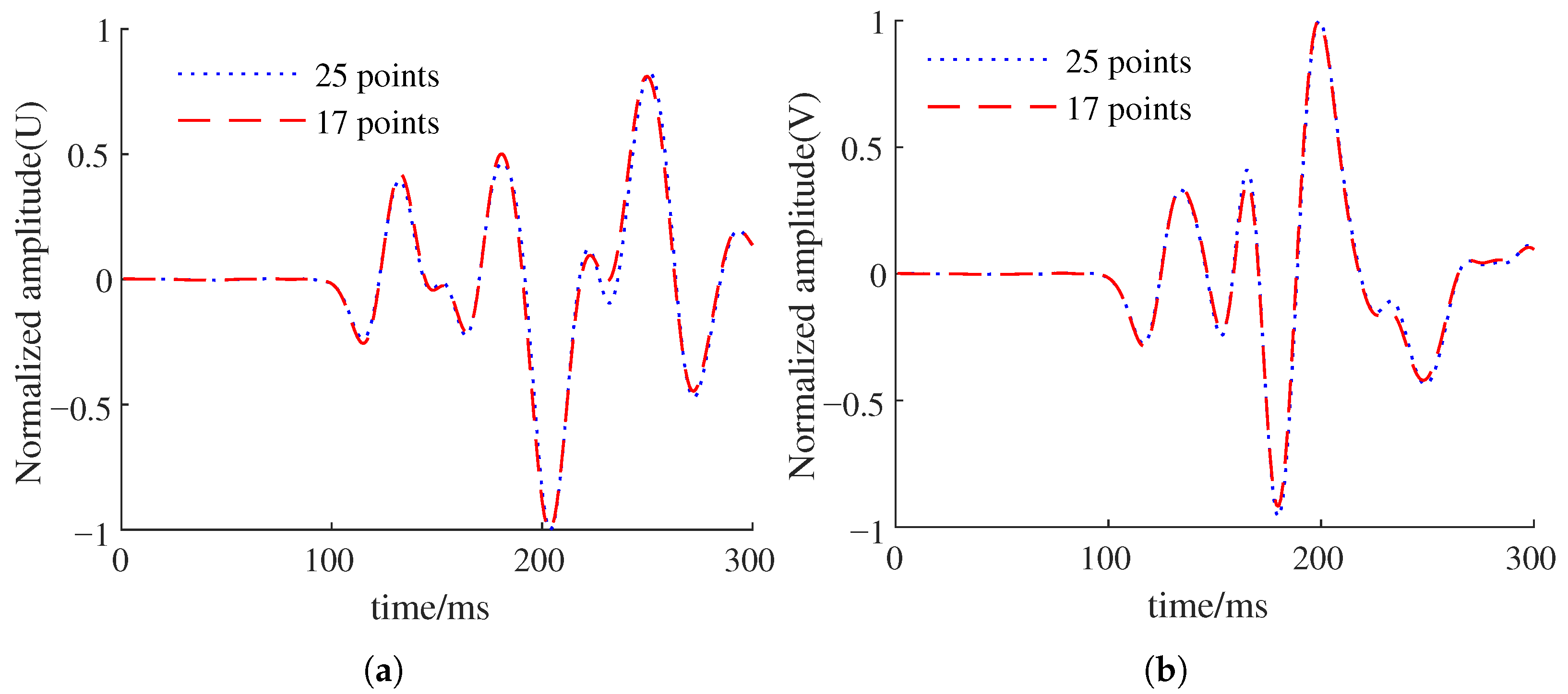
The spatial grid consists of N x = N z = 200 grid points with a uniform spacing of x = z = 3 m. The seismic source is a Ricker wavelet with a dominant frequency of 20 Hz, located at grid coordinates (100, 100), and the receiver is positioned at (120, 120). After adding a perfectly matched layer (PML) with a thickness of 20 grid points on each side, the actual computational domain size becomes 240 × 240 . The VTI medium anisotropy factors are ε = 0.5 and δ = 0.1 . The recording time is 0.3 s; in the frequency domain, this corresponds to 19 frequency points processed separately.
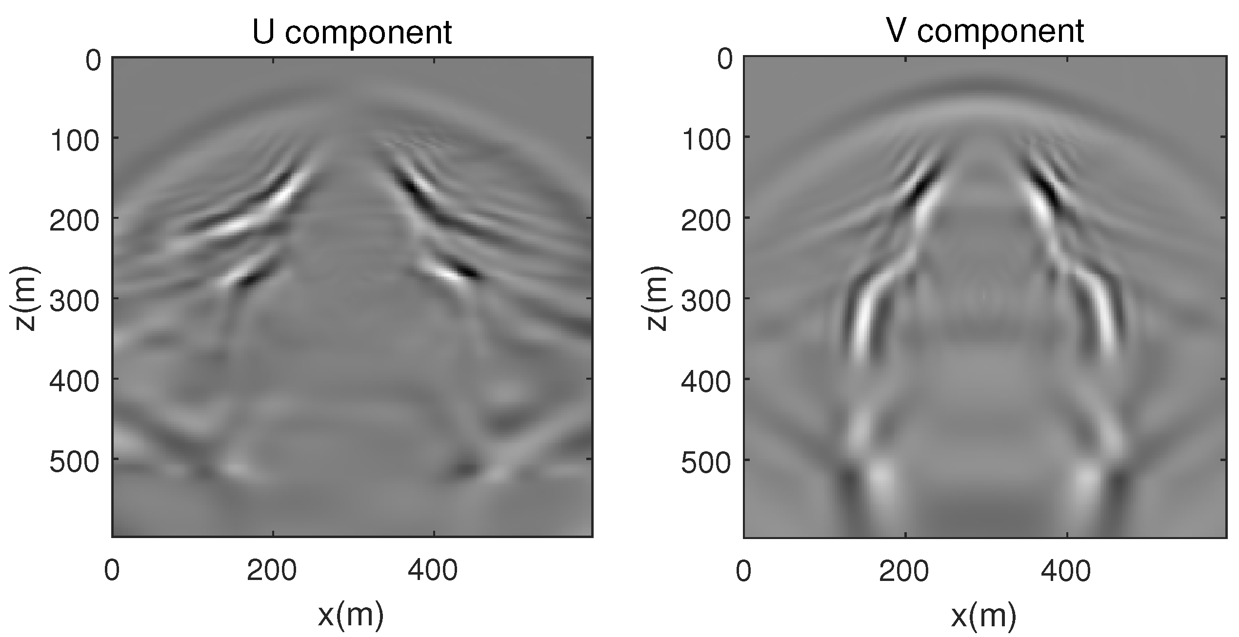
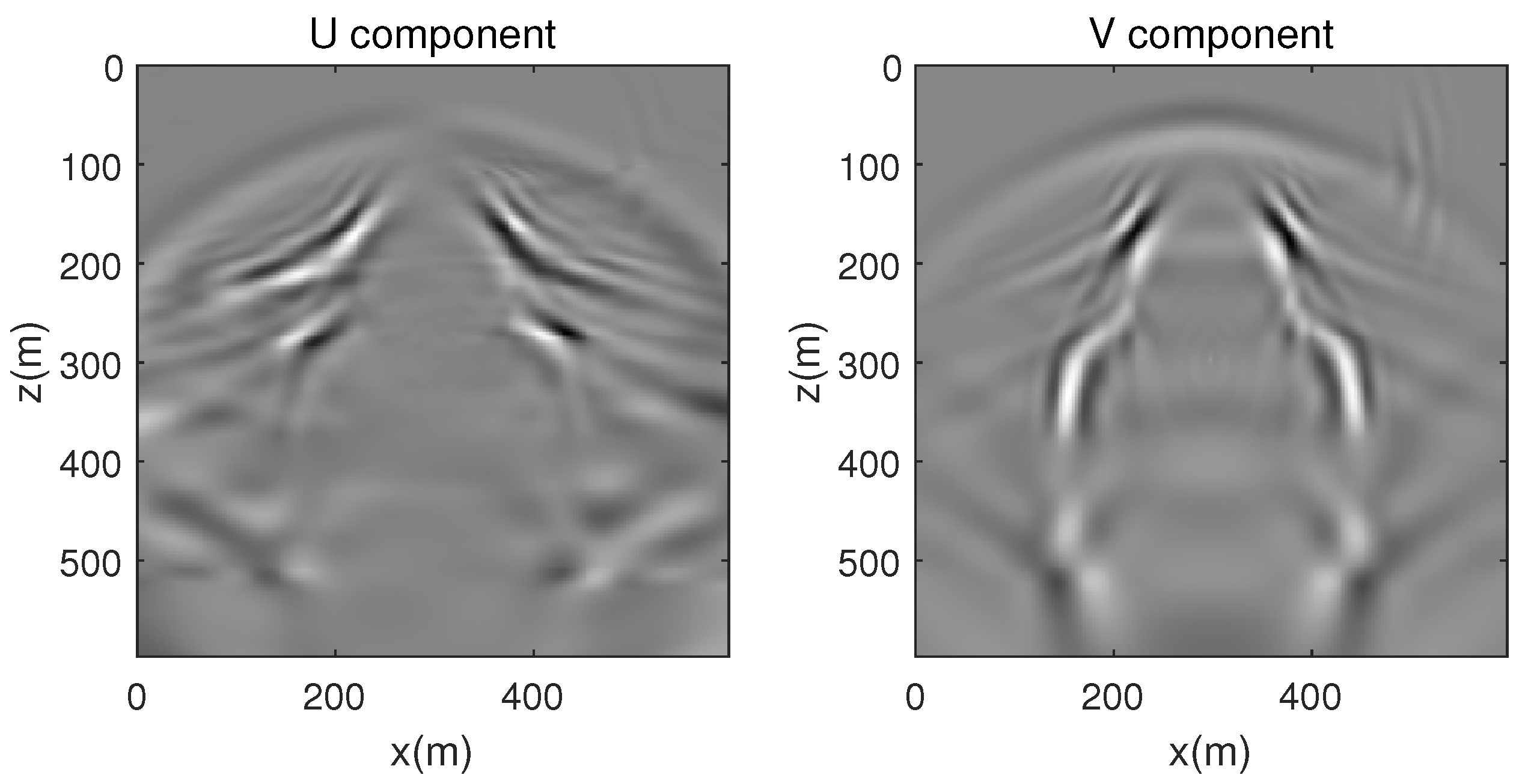
Figure 12, Figure 13 and Figure 14 present a portion of the simulation results. Figure 12 and Figure 13 show the U and V component snapshots at 175 ms. The wavefield is highly complex and exhibits distinct anisotropic characteristics. In the shallow, low-velocity layers of the model, the wavefield energy is stronger, whereas in the deeper, high-velocity layers, it appears weaker. This behavior reflects the influence of velocity variation in the VTI medium on wavefield propagation. Furthermore, the 17-point and 25-point finite-difference schemes yield consistent results in numerical simulations of complex media.
For further analysis, the U and V components at the receiver points are plotted for both the 17-point and 25-point finite-difference schemes, as illustrated in Figure 14. Except for minor discrepancies in individual peak amplitudes, the U and V components from both schemes align closely with each other in terms of travel time and first-arrival times.
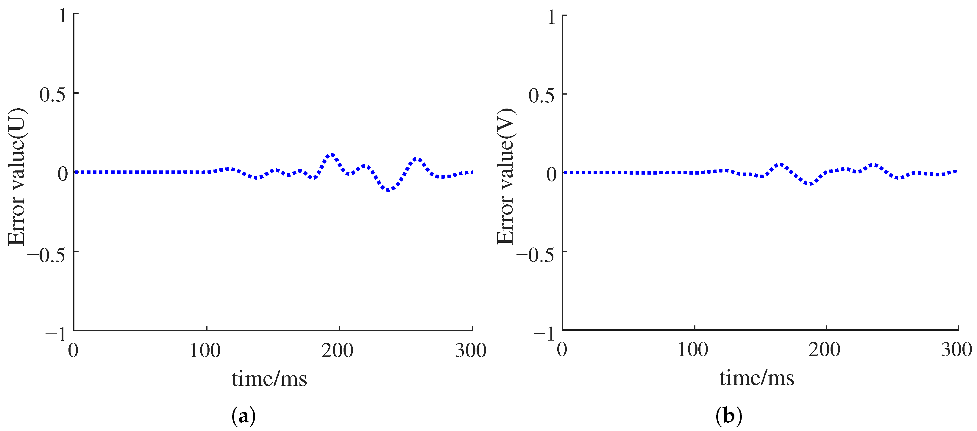
For the U component in Figure 15, the error statistics indicate a mean absolute error (MAE) of 0.0207, which is near zero, suggesting the absence of significant systematic bias and confirming the unbiased nature of the numerical solution—a positive indicator of convergence. The standard deviation (Std = 0.0356) and root mean square error (RMSE = 0.0356) are nearly identical, implying a relatively symmetric error distribution. Similar behavior is observed for the V component. The MAE is 0.0126, also near zero, reflecting negligible systematic bias and favorable convergence characteristics. The standard deviation (Std = 0.0258) and RMSE (0.0259) are nearly equal, again indicating a symmetric error distribution.
Overall, the error magnitudes remain within an acceptable range. The scheme exhibits good amplitude preservation, as evidenced by the symmetry between positive and negative peak errors, and demonstrates robust stability without anomalous divergence. The simulation accuracies of the two schemes remain comparable.

5. Discussion and Conclusions

To optimize the impedance matrix structure for frequency-domain elastic wave forward modeling in 2D VTI media—and thereby reduce memory requirements and enhance computational efficiency—we derive a simplified 17-point finite-difference scheme from the conventional 25-point scheme. This revised methodology redefines the difference operators for the partial derivative and acceleration terms in the elastic wave equations, reduces the number of grid points involved in the computation, and constructs the frequency-domain forward modeling matrix equation using sparse matrix compression techniques. Numerical simulations, validated through wavefield snapshots and comparisons of the U and V components at receiver locations, demonstrate that the 17-point scheme achieves comparable accuracy to the 25-point scheme while requiring 14 % less computation time and achieving a 25 % reduction in nonzero elements within the impedance matrix. Furthermore, computational efficiency can be further improved by adopting multi-shot sources and multi-core parallel computing based on domain decomposition strategies.

Author Contributions

Conceptualization, X.Y., C.Y. and Y.F.; methodology, X.Y., C.Y. and Y.F.; software, X.Y. with assistance from Y.F.; validation, X.Y. and C.Y.; data curation, C.Y. and X.Y.; writing—original draft preparation, X.Y.; writing—review and editing, X.Y., C.Y. and Y.F.; supervision, X.Y. and C.Y.; funding acquisition, X.Y. and Y.F. All authors have read and agreed to the published version of the manuscript.

Funding

This research is partially supported by the National Natural Science Foundation of China (No.12401551) and key scientific research projects of colleges and universities in Henan Province (No.24A170030).

Data Availability Statement

The data supporting the reported results are available on reasonable request to the first author.

Acknowledgments

All authors who contributed to this study are gratefully acknowledged.

Conflicts of Interest

The authors declare no conflicts of interest.

References

  1. Lysmer, J.; Drake, L.A. A finite element method for seismology. Methods Comput. Phys. 1972, 11, 181–216. [Google Scholar] [CrossRef]
  2. Thomsen, L. Weak elastic anisotropy. Geophysics 1986, 51, 1954–1966. [Google Scholar] [CrossRef]
  3. Pratt, R.G.; Worthington, M.H. Inverse theory applied to multi-source cross-hole tomography, part 1: Acoustic wave-equation method. Geophys. Prospect. 1990, 38, 287–310. [Google Scholar] [CrossRef]
  4. Pratt, R.G. Inverse theory applied to multi-source cross-hole tomography, part 2: Elastic wave-equation method. Geophys. Prospect. 1990, 38, 311–329. [Google Scholar] [CrossRef]
  5. Alkhalifah, T.; Tsvankin, I. Velocity analysis for transversely isotropic media. Geophysics 1995, 60, 1550–1566. [Google Scholar] [CrossRef]
  6. Charl-Hyun, J.; Shin, C.; Suh, J.H. An optimal 9-point, finite-difference, frequency-space, 2-D scalar wave extrapolator. Geophysics 1996, 61, 529–537. [Google Scholar] [CrossRef]
  7. Stekl, I.; Pratt, R.G. Accurate viscoelastic modeling by frequency-domain finite differences using rotated operators. Geophysics 1998, 63, 1779–1794. [Google Scholar] [CrossRef]
  8. Shin, C.; Sohn, H. A frequency-space 2-D scalar wave extrapolator using extended 25-point finite-difference operator. Geophysics 1998, 63, 289–296. [Google Scholar] [CrossRef]
  9. Pratt, R.G. Seismic waveform inversion in the frequency domain, part 1: Theory and verification in a physical scale model. Geophysics 1999, 64, 888–901. [Google Scholar] [CrossRef]
  10. Min, D.-J.; Shin, C.; Kwon, B.-D.; Chung, S. Improved frequency-domain elastic wave modeling using weighted-averaging difference operators. Geophysics 2000, 65, 884–895. [Google Scholar] [CrossRef]
  11. Sirgue, L.; Pratt, R.G. Efficient waveform inversion and imaging: A strategy for selecting temporal frequencies. Geophysics 2004, 69, 231–248. [Google Scholar] [CrossRef]
  12. Wu, G.C.; Liang, K. Quasi P-wave forward modeling in frequency-space domain in VTI media. Oil Geophys. Prospect. 2005, 40, 535–545. (In Chinese) [Google Scholar]
  13. Wu, G.-Z.; Luo, C.-M.; Liang, K. Frequency-space domain finite difference numerical simulation of elastic wave in TTI media. J. Jilin Univ. (Earth Sci. Ed.) 2007, 37, 1023–1033. [Google Scholar] [CrossRef]
  14. Operto, S.; Virieux, J.; Ribodetti, A.; Anderson, J.E. Finite-difference frequency-domain modeling of viscoacoustic wave propagation in 2D tilted transversely isotropic (TTI) media. Geophysics 2009, 74, T75–T95. [Google Scholar] [CrossRef]
  15. Kostin, V.I.; Tcheverda, V.A.; Reshetova, G.V.; Tcheverda, V.V. A finite-difference method for the numerical simulation of seismic wave propagation through multiscale media. Inst. Comput. Math. Math. Geophys. 2011, 230, 321–329. [Google Scholar]
  16. Rodriguez, I.V.; Bonar, D.; Sacchi, M. Microseismic data denoising using a 3C group sparsity constrained time-frequency transform. Geophysics 2012, 77, V21–V29. [Google Scholar] [CrossRef]
  17. Gu, B.; Liang, G.; Li, Z. A 21-point finite difference scheme for 2D frequency-domain elastic wave modelling. Explor. Geophys. 2013, 44, 156–166. [Google Scholar] [CrossRef]
  18. Fauchard, C.; Antoine, R.; Bretar, F.; Lacogne, J.; Fargier, Y.; Maisonnave, C.; Guilbert, V.; Marjerie, P.; Thérain, P.-F.; Dupont, J.-P.; et al. Assessment of an ancient bridge combining geophysical and advanced photogrammetric methods: Application to the Pont De Coq, France. J. Appl. Geophys. 2013, 98, 100–112. [Google Scholar] [CrossRef]
  19. Gosselin-Cliche, B.; Giroux, B. 3D frequency-domain finite-difference viscoelastic-wave modeling using weighted average 27-point operators with optimal coefficients. Geophysics 2014, 79, T169–T188. [Google Scholar] [CrossRef]
  20. Fomel, S.; Ying, L.X.; Song, X.L. Seismic wave extrapolation using low rank symbol approximation. Geophys. Prospect. 2012, 61, 526–536. [Google Scholar] [CrossRef]
  21. Lipnikov, K.; Manzini, G.; Shashkov, M. Mimetic finite difference method. J. Comput. Phys. 2014, 257, 1163–1227. [Google Scholar] [CrossRef]
  22. Ping, P.; Xu, Y.; Zhang, Y.; Yang, B. Seismic wave modeling in viscoelastic VTI media using spectral element method. Science 2014, 27, 553–565. [Google Scholar] [CrossRef]
  23. Hobiger, M.; Wegler, U.; Shiomi, K.; Nakahara, H. Coseismic and post-seismic velocity changes detected by Passive Image Interferometry: Comparison of one great and five strong earthquakes in Japan. Geophys. J. Int. 2016, 205, 1053–1057. [Google Scholar] [CrossRef]
  24. Boada, A.; Paolini, C.; Castillo, J.E. High-order mimetic finite differences for anisotropic elliptic equations. Comput. Fluids 2020, 213, 104746. [Google Scholar] [CrossRef]
  25. Sethi, H.; Hoxha, F.; Shragge, J.; Tsvankin, I. Modeling 3-D anisotropic elastodynamics using mimetic finite differences and fully staggered grids. Comput. Geosci. 2023, 27, 793–804. [Google Scholar] [CrossRef]
  26. Dong, S.; Chen, J. Affine 25-point scheme for high-accuracy numerical simulation of frequency-domain acoustic wave equation. Chin. J. Geophys. 2024, 67, 3859–3873. [Google Scholar] [CrossRef]
  27. Shin, Y. Tensor-Train-Based Elastic Wavefield Decomposition in VTI Media. Appl. Sci. 2026, 16, 569. [Google Scholar] [CrossRef]
  28. Martin, G.S.; Wiley, R.; Marfurt, K.J. Marmousi2: An elastic upgrade for Marmousi. Lead. Edge 2006, 25, 156–166. [Google Scholar] [CrossRef]
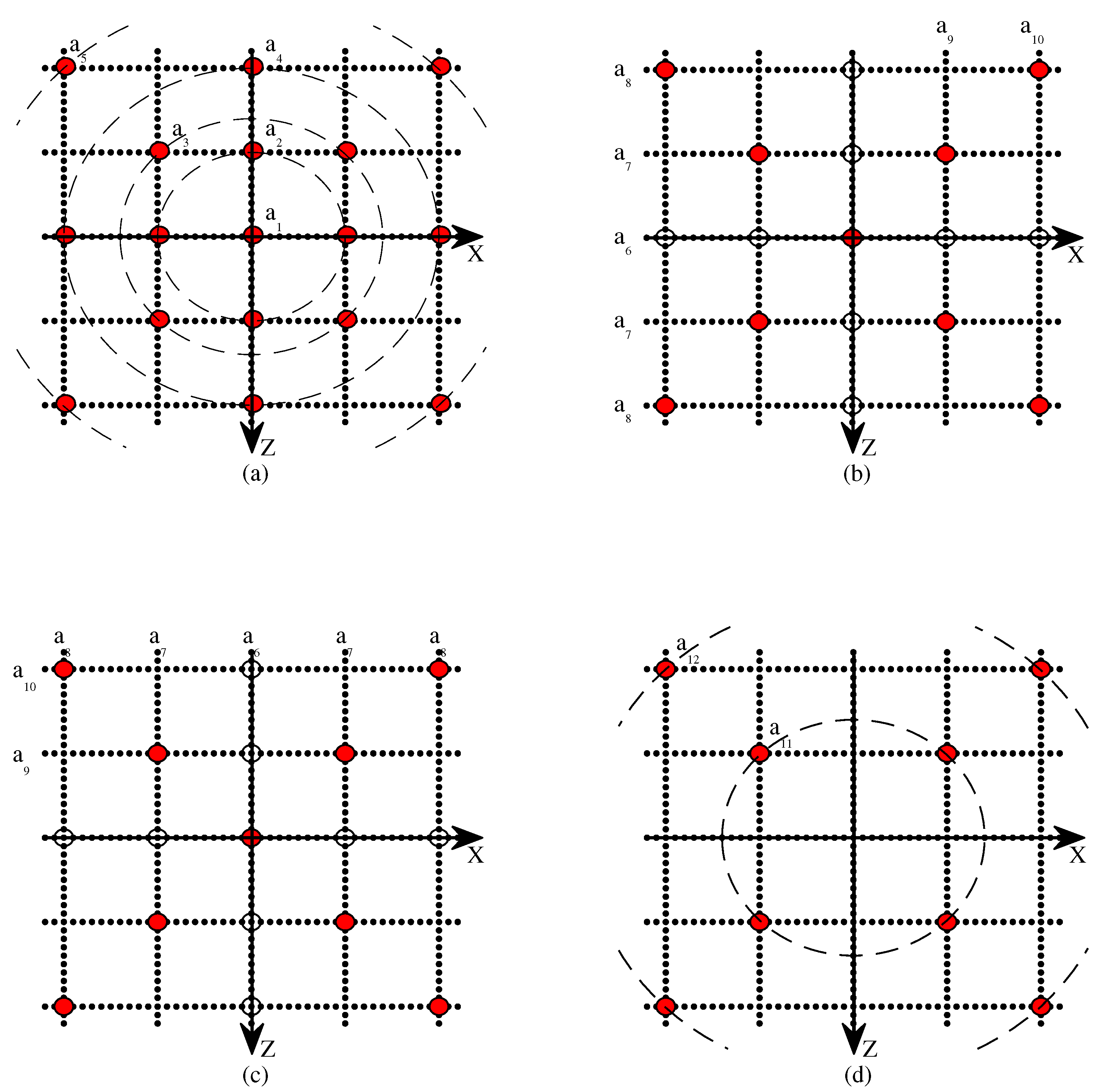
Figure 1. Seventeen-point finite-difference scheme weighted discretization diagram (a) is the coefficient distribution of acceleration term U; (bd) correspond to coefficient distributions of 2 U x 2 , 2 U z 2 , 2 U x z , respectively. The black circles and red filled circles represent the grid points required for differential calculations, while the dashed circles represent grid points that are at the same distance from the center point and use the same coefficients. The specific method of adding coefficients is shown in formulas (2)–(5).
Processes 14 01283 g001
Figure 2. Dispersion curves of 17-point finite-difference scheme (Poisson ratio = 0.25).
Processes 14 01283 g002
Figure 3. Dispersion curves of 25-point finite-difference scheme (Poisson ratio = 0.25).
Processes 14 01283 g003
Figure 4. Snapshot at 125 ms of 17-point finite-difference scheme.
Processes 14 01283 g004
Figure 5. Snapshot at 125 ms of 25 point finite-difference scheme.
Processes 14 01283 g005
Figure 6. Comparison of U , V components at the receiver (a,b) of simple VTI medium model.
Processes 14 01283 g006
Figure 7. Example of nonzero element in impedance matrices for 17-point (a) and 25-point (b) finite-difference scheme.
Processes 14 01283 g007
Figure 8. Double-layer VTI medium model.
Processes 14 01283 g008
Figure 9. Snapshot at 175 ms of 17-point scheme about two-layer VTI medium.
Processes 14 01283 g009
Figure 10. Marmousi model ( V p ).The black box in the figure indicates the area for numerical simulation.
Processes 14 01283 g010
Figure 11. Partions of Marmousi model.
Processes 14 01283 g011
Figure 12. Snapshot at 175 ms of 17-point finite-difference scheme.
Processes 14 01283 g012
Figure 13. Snapshot at 175 ms of 25 point finite-difference scheme.
Processes 14 01283 g013
Figure 14. Comparison of U , V components at the receiver (a,b).
Processes 14 01283 g014
Figure 15. Errors of U , V components at the receiver (a,b).
Processes 14 01283 g015
Table 1. Weighting coefficients.
CoefficientsValueCoefficientsValue
a 1 0.4995 a 7 0.2375
a 2 0.1154 a 8 −0.0182
a 3 0.0183 a 9 0.8430
a 4 0.1031 a 10 0.3512
a 5 0.0001 a 11 1.2984
a 6 0.7724 a 12 −0.0256
Table 2. Comparison between 17-point and 25-point finite-difference scheme (with the result of 25-point finite-difference scheme as 1).
Finite-Difference Scheme17-Point 25-Point
Value Proportion Value Proportion
Nonzero elements1,976,0800.75812,606,5121
Memory usage of impedance matrix5.57 M0.73067.32 M1
Time in solving the Equation (7)6.3233 s0.86647.3156 s1
Memory usage3447.36 M0.75954538.83 M1
Table 3. Parameters of two-layer VTI medium.
Parameters V p /(m · s−1) V s /(m · s−1) ε δ ρ /(kg · m−3)
First layer300020000.50.12000
Second layer400030000.3−0.12500
Disclaimer/Publisher’s Note: The statements, opinions and data contained in all publications are solely those of the individual author(s) and contributor(s) and not of MDPI and/or the editor(s). MDPI and/or the editor(s) disclaim responsibility for any injury to people or property resulting from any ideas, methods, instructions or products referred to in the content.