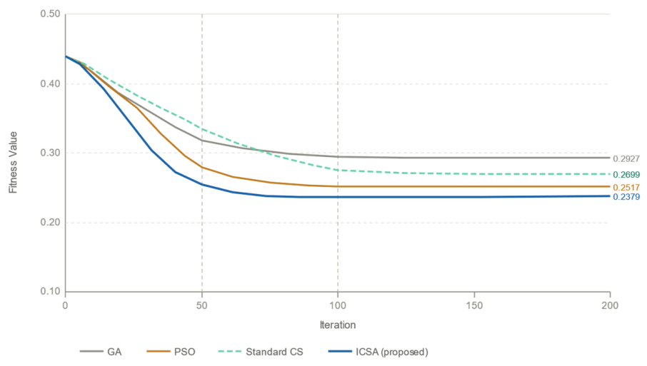
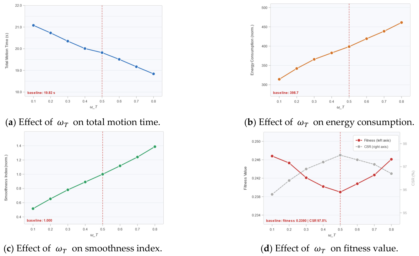
6.3.1. Effectiveness Validation of the ATBSC
To evaluate the effectiveness of the proposed ATBSC framework, this section presents three groups of comparative experiments using all 80 test scenarios, with each comparison method independently executed 20 times under each scenario to obtain statistically significant performance comparison results. A systematic evaluation is conducted from multiple dimensions.
- (1)
Comprehensive Comparison of ATBSC with Traditional Pose-Setting Methods
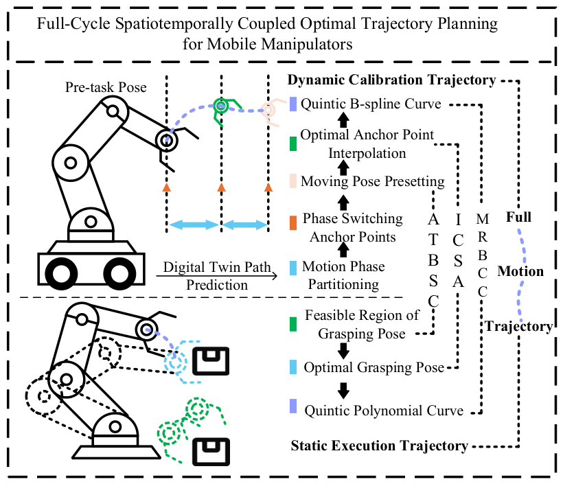
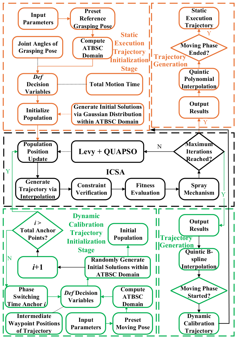
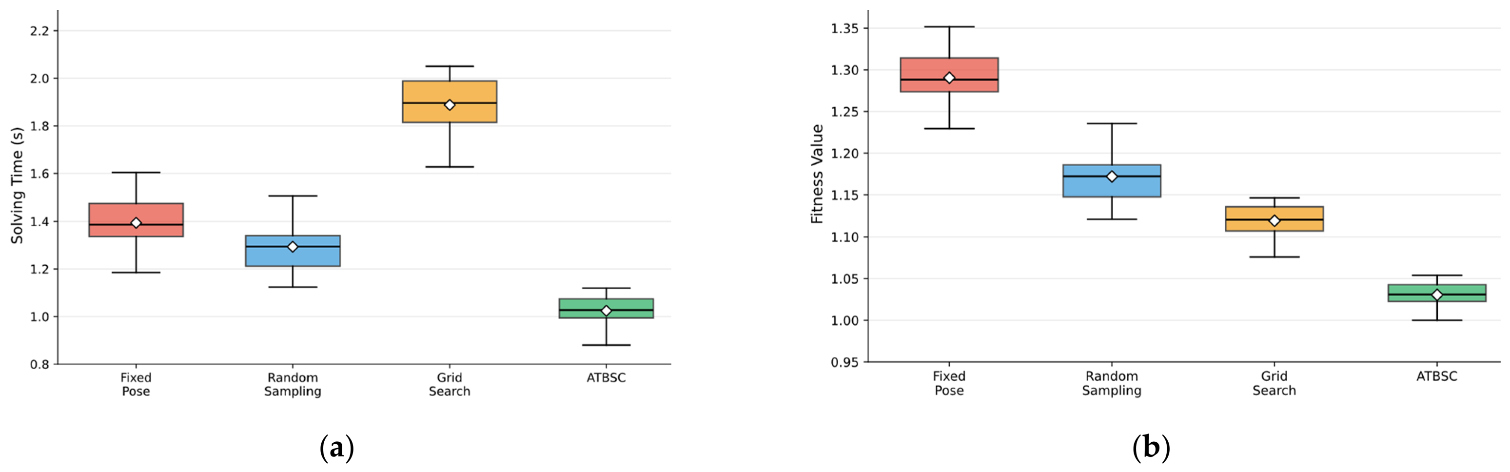
To validate the advantages of ATBSC over traditional pose-setting methods, this experiment compares four methods: (a) Fixed Pose Method—directly adopting the reference configuration solved by IK as the initial solution; (b) Random Sampling Method—randomly sampling within the kinematically admissible space to generate the initial population; (c) Grid Search Method—uniform grid partitioning and sampling within the joint space; (d) ATBSC. The solving time, fitness value, convergence iteration count, constraint satisfaction rate, and trajectory quality metrics from 20 independent repeated experiments are recorded as shown in
Table 4 and
Figure 10.
As shown in
Table 4 and
Figure 10, under the simulation conditions of this study, ATBSC consistently outperforms the three baseline methods across all evaluated metrics.
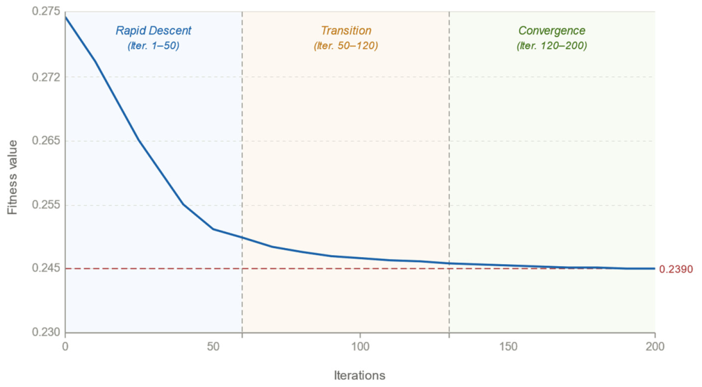
In terms of solving time, ATBSC averages 1.0255 s, a 27.5% reduction over the Fixed Pose Method (1.4145 s) and a 45.8% reduction over the Grid Search Method (1.8920 s). For fitness value, ATBSC achieves 1.0312, a 20.5% improvement over the Fixed Pose Method (1.2964). Convergence requires 91.6 iterations on average, 51.0% fewer than the baseline methods in the simulation. The constraint satisfaction rate of 97.5% is markedly higher than the 72.0% of the Fixed Pose Method under these simulation conditions. In terms of trajectory quality, ATBSC reduces the total motion time to 19.82 s (an 11.7% reduction) and total energy consumption to 398.7 (a 17.9% reduction) relative to the Fixed Pose Method in the tested scenarios.
- (2)
Search Space Constraint and Deviation Controllability Validation
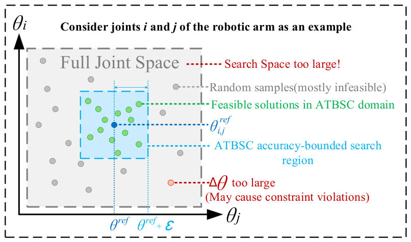
The core advantage of ATBSC lies in reducing the effective search space through geometry-inspired bounded constraints while ensuring that the deviation between the optimized solution and the reference configuration remains within a bounded range. This experiment validates the search space reduction effectiveness and deviation controllability.
As shown in
Table 5, ATBSC (
) compresses the search space to 0.12% of the original full joint space, with a valid solution density reaching 84.7%, which is 36.8 times that of the full space (2.3%), indicating that the search space is effectively focused on high-quality solution regions; ATBSC requires only an average of 1.18 samples to obtain a feasible solution, whereas the full space requires 43.5 samples, representing an efficiency improvement of 36.9 times.
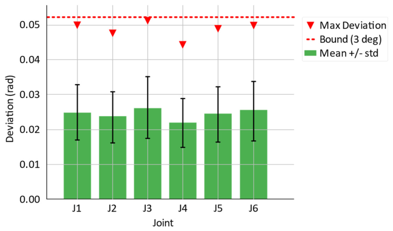
To validate the deviation controllability of ATBSC, we conducted 100 independent repeated experiments.
Figure 11 presents the statistical distribution of deviations for each joint. The results demonstrate that across all 100 runs, the deviations of all six joints never exceeded the preset accuracy boundary
rad (3°), and the mean deviation of each joint ranges between 0.0219~0.0261 rad, approximately 42~50% of the boundary value, indicating that the optimization process maintains a safety margin while fully utilizing the search space.
Table 6 compares the deviation performance of three methods: ATBSC reduces the average deviation from 0.0892 rad of the unconstrained method to 0.0243 rad, a reduction of 72.8%; the maximum deviation is reduced from 0.1847 rad to 0.0512 rad, a reduction of 72.3%. This demonstrates that ATBSC not only significantly reduces the mean deviation but more importantly substantially narrows the deviation distribution range, ensuring stable and controllable quality of optimized solutions.
- (3)
Accuracy Boundary Parameter Analysis
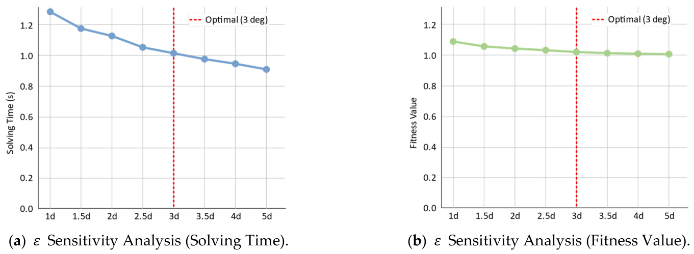
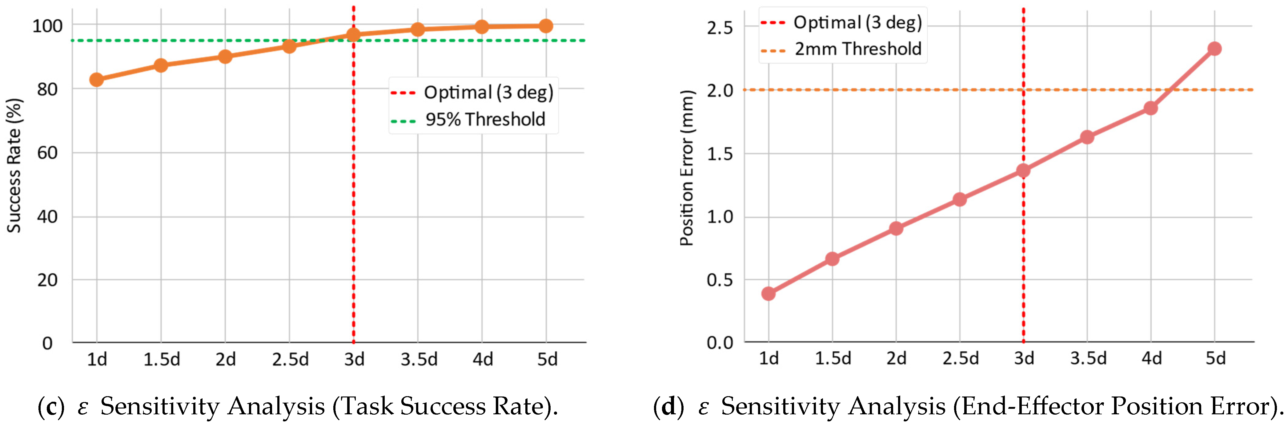
The accuracy boundary of the “Grasping Pose” determines the search range of the ATBSC accuracy-bounded search region. This experiment systematically tests the impact of values ranging from 1° to 5° on algorithm performance.
As shown in
Figure 12, as
increases, the solving time gradually decreases from 1.28 s to 0.91 s, representing an efficiency improvement of 28.9%. The fitness value decreases from 1.089 to 1.019, indicating improved solution quality. However, the end-effector position error increases from 0.42 mm to 2.31 mm. Through comprehensive analysis,
represents the optimal trade-off between efficiency and precision: at this point, the success rate reaches 97%, the position error is controlled within 1.38 mm, and the orientation error is only 0.39°, satisfying the precision requirements of most industrial applications. When
is too small (<2°), the constrained search space leads to decreased success rate; when
is too large (>4°), although computational efficiency slightly improves, the position error exceeds the 2 mm industrial precision threshold.
6.3.2. Effectiveness Validation of the MRBCC Framework
- (1)
Comparison of MRBCC with Traditional Constraint Methods
To validate the advantages of MRBCC over traditional constraint methods for the CMM, this experiment compares three methods: (a) No Inertial Constraint method (NIC)—considering only kinematic boundary constraints while ignoring inertial disturbances generated by platform motion; (b) Kinematic Constraints Only method (KCO)—adopting the kinematic constraint system from the Sequential Quadratic Programming-based method proposed by Li et al. [
8], which constrains joint velocity and acceleration boundaries but does not explicitly model or compensate for inertial disturbance torques; (c) MRBCC. The experiments are conducted over the complete mobile platform motion cycle (including acceleration, constant-speed, turning, and braking phases) across all 80 test scenarios, with each scenario independently repeated 20 times, measuring the end-effector position error, orientation error, and constraint violation rate at the platform standstill moment
.
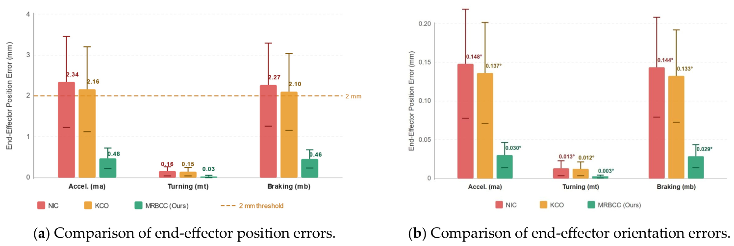
As shown in
Table 7 and
Figure 13, MRBCC outperforms the comparison methods across all motion phases. During the acceleration phase (ma), MRBCC reduces the end-effector position error from 2.34 mm of the NIC method to 0.48 mm, a reduction of 79.7%; compared to the KCO method (2.16 mm), the reduction is 78.0%. Notably, the position errors of NIC and KCO are nearly identical (2.34 mm vs. 2.16 mm, a difference of only 7.7%). This is physically expected: neither method applies inertial disturbance torque compensation, and their end-effector errors are governed by the same steady-state response
. The kinematic constraints in KCO can reduce trajectory oscillations and improve smoothness (manifested as a modest 7.7% reduction), but cannot eliminate the persistent joint deviations driven by uncompensated inertial torques. During the turning phase (mt), the mean centripetal acceleration generated by platform turning is
m/s
2, which is substantially lower than the mean linear acceleration
m/s
2 of the other phases, resulting in proportionally smaller inertial disturbances across all methods. Nevertheless, MRBCC still reduces the position error to 0.03 mm. During the braking phase (mb), MRBCC achieves a position error of 0.46 mm, representing reductions of 79.8% and 78.1% compared to the NIC and KCO methods, respectively. Regarding orientation error, the mean orientation errors of MRBCC during the acceleration, turning, and braking phases are 0.030°, 0.003°, and 0.029°, respectively, all well below the 1° industrial precision requirement. Regarding constraint violation rate, MRBCC maintains a consistent violation rate of 2.5 ± 0.6% across the three motion phases, below the 5% threshold, achieving a global constraint satisfaction rate of 97.5%. In contrast, NIC and KCO do not impose the phase-specific dynamic coupling constraints defined in Equations (15), (18) and (20), and therefore cannot provide formal guarantees of dynamic compliance.
The above results indicate that, under the simulation conditions of this study, MRBCC outperforms the comparison methods across all motion phases, indicating that the manipulator is able to reach the preset “Moving Pose” with near-zero residual velocity and acceleration at the platform standstill moment, thereby providing the deterministic initial conditions required by the full-cycle framework for the subsequent static execution trajectory. The residual errors (0.46–0.48 mm) across the three motion phases stem from first-order linearization of the coupled dynamics. These errors are strictly bounded by the ATBSC ().
- (2)
MRBCC Inertial Coupling Coefficient Robustness Analysis
The inertial coupling coefficients
are key parameters of the MRBCC framework. As shown in
Table 2, these coefficients exhibit pronounced joint specificity: in the linear acceleration direction, from
(J5, lowest sensitivity) to
(J2, highest sensitivity); in the centripetal acceleration direction, from
(J4) to
(J1). In practical applications, exact values may deviate from the analytical estimates due to payload variations, unmodeled link flexibility, and linearization approximation errors. This experiment evaluates the robustness of the MRBCC framework to such parameter uncertainties by introducing a proportional perturbation factor
uniformly applied to all joints (
), where
corresponds to the exact analytical values in
Table 2;
represents underestimation (e.g., discrepancies between no-load and loaded conditions);
represents overestimation (conservative constraint tightening). Since the disturbance mechanisms for the linear acceleration and centripetal acceleration phases differ, the two coefficient groups are analyzed separately: Experiment 1 fixes
and sweeps
to assess the robustness of the linear acceleration direction coefficients
(applicable to the acceleration and braking phases); Experiment 2 fixes
and sweeps
over the same range to assess the robustness of the centripetal acceleration direction coefficients
(turning phase). Each
level is evaluated with 20 independent repetitions across all 80 test scenarios, recording end-effector position error, constraint satisfaction rate, and composite performance index.
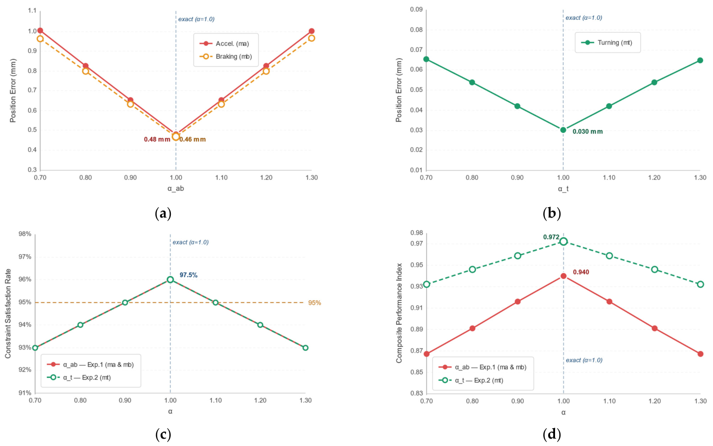
As shown in
Figure 14a, in Experiment 1, the end-effector position errors during the acceleration and braking phases exhibit a symmetric U-shaped relationship with
, reaching the minimum at
(exact analytical value): 0.48 mm (ma) and 0.46 mm (mb). As
deviates from 1.00, the errors increase symmetrically in both directions: at
(30% underestimation), errors increase to 1.00 mm (ma) and 0.96 mm (mb); at
(30% overestimation), errors similarly increase to 1.00 mm and 0.97 mm. This symmetry confirms that both underestimation and overestimation of the coupling coefficients lead to comparable performance degradation—underestimation results in insufficient disturbance compensation, while overestimation results in over-tightened constraints on the calibration trajectory, reducing its flexibility.
As shown in
Figure 14b, in Experiment 2, the turning phase error likewise exhibits a symmetric pattern centered at
(0.030 mm), increasing to 0.066 mm and 0.065 mm at
and
, respectively. The absolute error values are smaller than those in the linear acceleration phases, consistent with the lower centripetal acceleration magnitudes in
Table 1, indicating that the turning phase coefficients
have less stringent precision requirements compared to the linear acceleration phase coefficients.
As shown in
Figure 14c, the constraint satisfaction rate exhibits a symmetric inverted U-shaped relationship with
, with both experimental groups peaking at
(97.5%) and monotonically decreasing as
deviates from 1.00. For both the
and
groups, the satisfaction rate remains above 96.0% within
(exact value ± 10%); and above 94.5% within
(±20%). This demonstrates that even under moderate uncertainty in coupling coefficient estimates, the MRBCC framework maintains acceptable constraint compliance.
As shown in
Figure 14d, the composite performance index (simultaneously accounting for position error and constraint satisfaction rate) confirms that both experimental groups reach the optimum at
(0.940 for the
group; 0.972 for the
group). The
curve outperforms the
curve at all
values, reflecting the lower absolute contribution of centripetal disturbances to overall performance during platform operation. The flat optimal region near
—with the
composite index remaining above 0.91 within
—further validates the practical robustness of the analytical coefficient derivation in
Table 2: setting
within a physically reasonable range near the analytical values is sufficient to ensure effective operation of the MRBCC framework.
- (3)
Temporal Error Analysis and Ablation Experiment
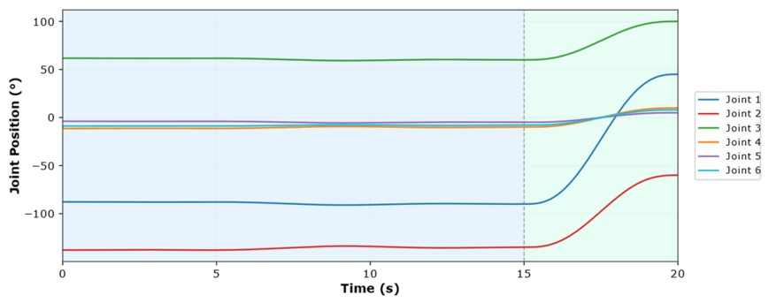
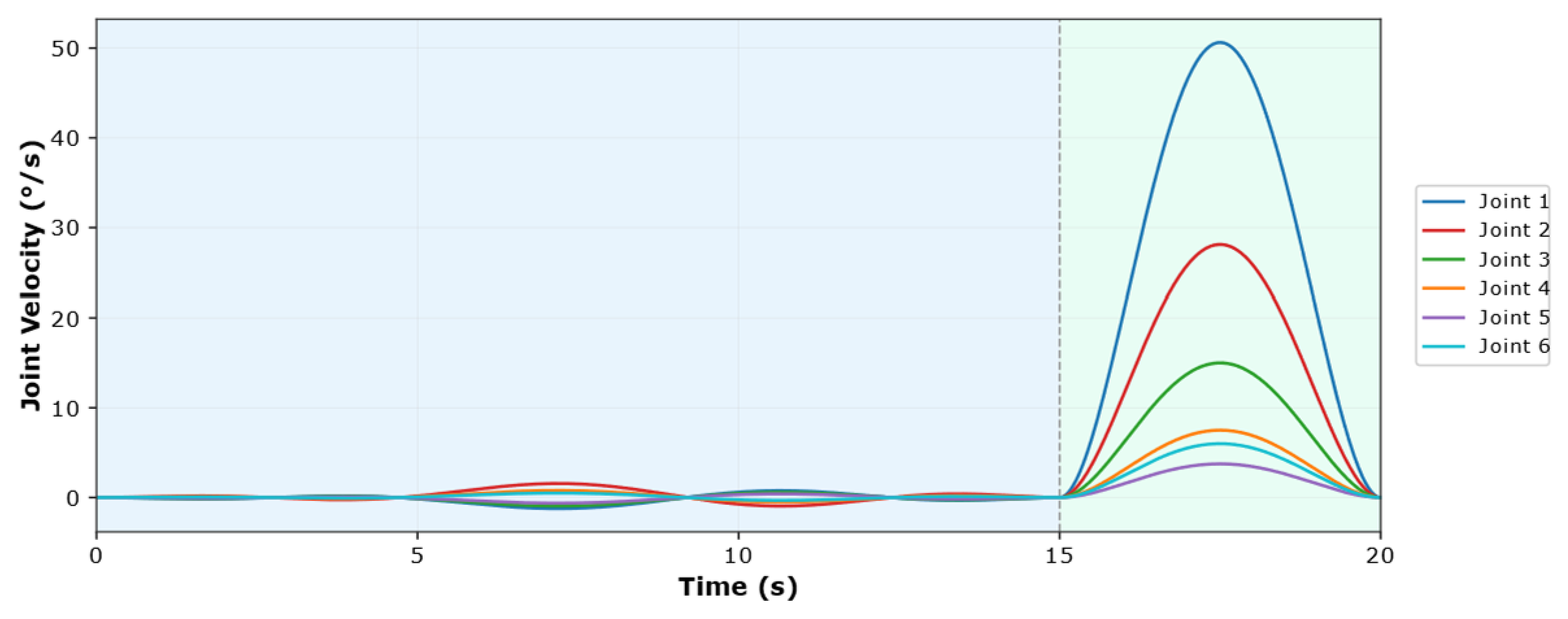
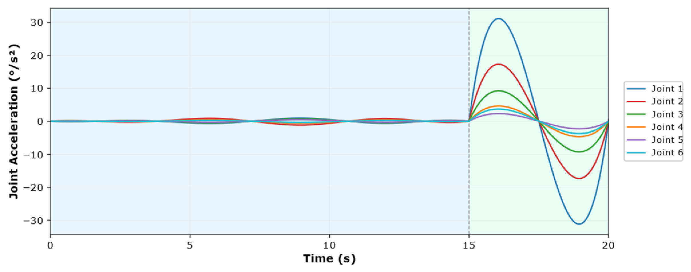
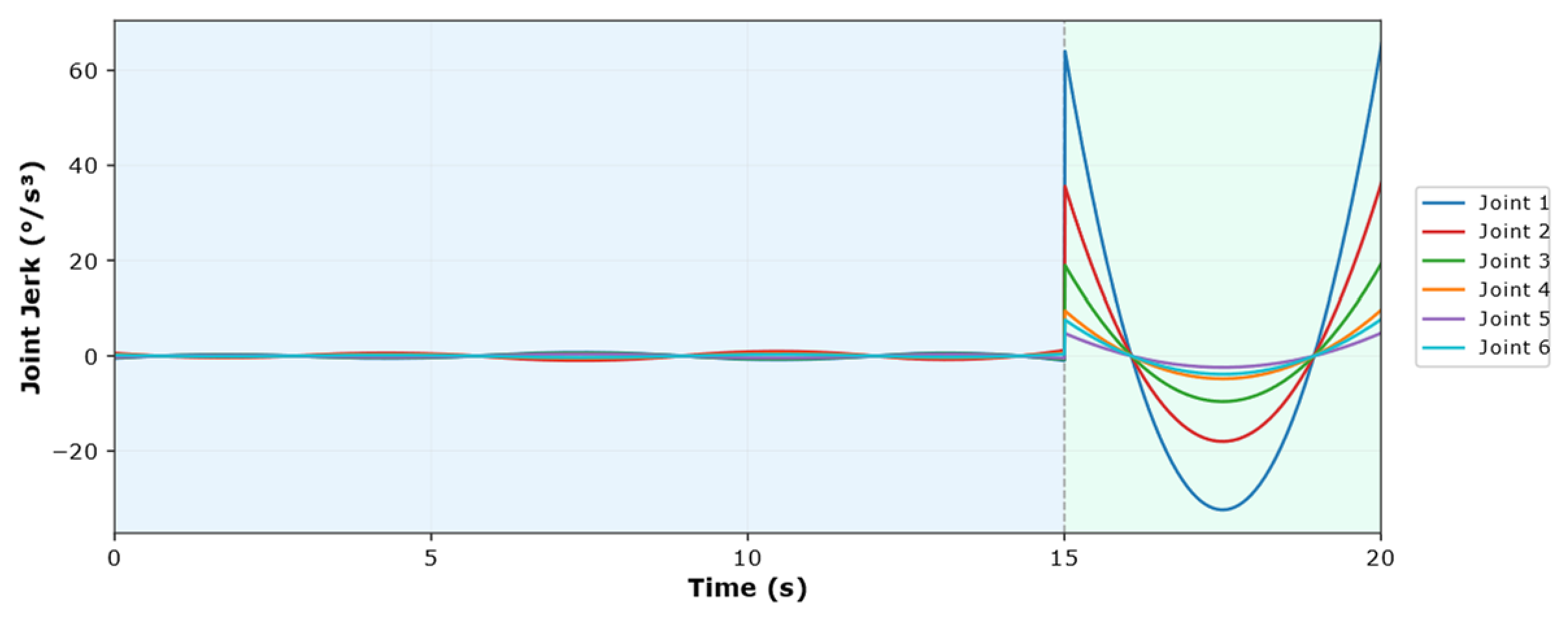
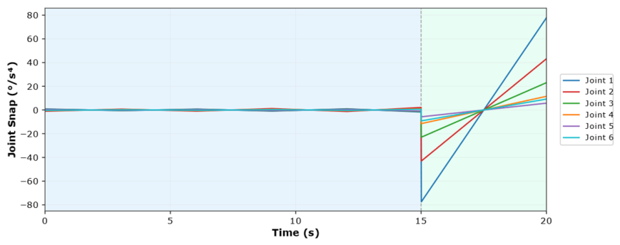
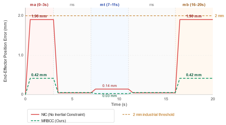
To further validate the suppression effectiveness of MRBCC on inertial disturbances throughout the complete motion cycle of the mobile platform, this experiment sets up a fixed test scenario with a total motion time of 20 s, comprising 5 sequentially executed phases: acceleration (ma, 0–3 s, m/s2), constant-speed (ms, 3–7 s), turning (mt, 7–11 s, rad/s), constant-speed (ms, 11–16 s), and braking (mb, 16–20 s, m/s2). The end-effector position error temporal curve throughout the entire Moving Phase is recorded, and the contribution of each constraint component is analyzed through ablation experiments.
As shown in
Figure 15, the NIC method produces peak position errors of 1.90 mm during the acceleration (ma) and braking (mb) phases, approaching but still within the 2 mm industrial precision threshold. The peak during the turning phase (mt) is only 0.14 mm, consistent with the lower centripetal acceleration (
m/s
2) at the operating speed of the mobile platform. In contrast, the MRBCC method keeps the end-effector error within 0.42 mm throughout the entire Moving Phase (0.42 mm during the ma and mb phases; 0.03 mm during the mt phase), providing substantially greater precision margins below the industrial threshold.
As shown in the ablation experiment results (
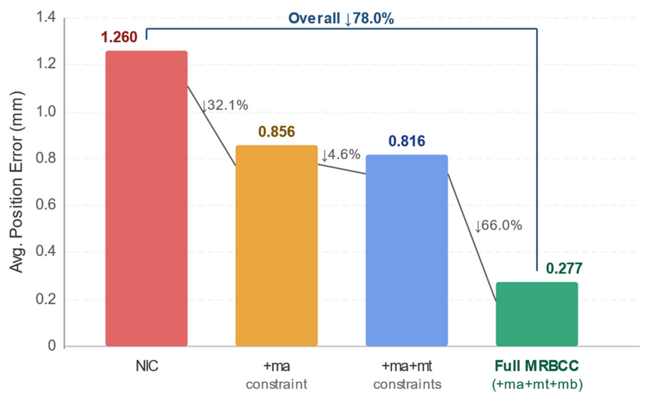
Figure 16), starting from the NIC baseline (mean error across dynamic phases: 1.26 mm), adding the acceleration phase constraint (+ma) reduces the error to 0.856 mm, a reduction of 32.1%; further adding the turning phase constraint (+ma+mt) marginally reduces the error to 0.816 mm (a further reduction of 4.6%), because the centripetal disturbance during the turning phase is relatively small at the operating speed of the mobile platform; adding the braking phase constraint to complete the full MRBCC framework yields the largest reduction, bringing the error down to 0.277 mm (a further reduction of 66.0%), because the braking phase has the longest duration (4 s) in this scenario and thus the highest cumulative disturbance contribution. The full MRBCC framework achieves an overall reduction of 78.0% relative to NIC.
The ablation results confirm that all three constraint components make positive contributions, with their relative magnitudes reflecting the disturbance intensity and phase duration of each motion phase: the braking phase constraint contributes the most due to its long duration; the acceleration phase constraint contributes significantly due to comparable linear acceleration magnitudes; and the turning phase constraint contributes the least due to the lower centripetal acceleration at the operating speed of the mobile platform. This validates the necessity of the phase-specific constraint design in the MRBCC framework.
- (4)
Comparison with Mobile Manipulator-Specific Disturbance Rejection Methods
This section compares MRBCC with two representative mobile manipulator-specific disturbance rejection control-layer baseline methods: (a) Disturbance Observer-Based Control (DOB), implemented following the coupled dynamics modeling framework of Zhou et al. [
3], in which joint-level disturbance observers estimate inertial disturbance torques via low-pass filtering (cutoff frequency 10 Hz) and apply real-time compensation; (b) Model Predictive Disturbance Compensation (MPC-PDC), implemented following the framework of Tao et al. [
22], which utilizes DT-predicted platform motion time series and solves a quadratic programming tracking problem at each 5 ms control cycle (prediction horizon: 10 steps, 6 joints). The experiments are conducted across all 80 test scenarios, with 20 independent repetitions per scenario. It should be noted that MRBCC operates at the planning layer: the analytically derived inertial coupling constraints from
Table 2 are embedded into the dynamic calibration trajectory prior to execution, causing the manipulator to converge to
at
by design, with zero online computation during execution. DOB and MPC-PDC operate at the control layer: they estimate or predict disturbance torques at each control cycle and apply compensating joint commands. These two paradigms address the same disturbance problem at different architectural layers and are complementary rather than competing; accordingly, the following comparison is organized around the dimensions where genuine differences exist.
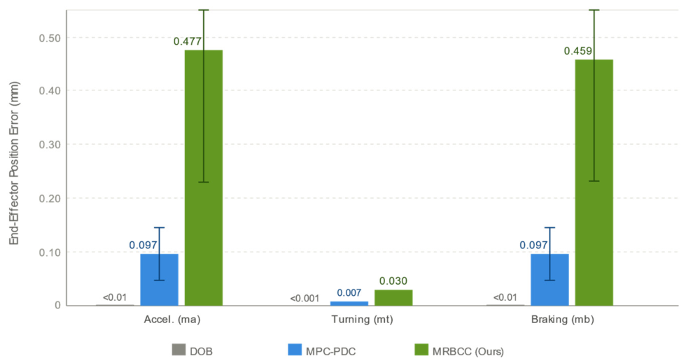
As shown in
Figure 17 and
Table 8, under planned platform disturbances, DOB achieves near-zero position errors across all three motion phases (ma: 0.002 mm; mt: <0.001 mm; mb: 0.002 mm), and MPC-PDC likewise achieves very low errors (ma/mb: 0.097 mm; mt: 0.007 mm). MRBCC retains larger residuals (ma: 0.477 mm; mb: 0.459 mm; mt: 0.030 mm); for the dominant linear acceleration phases, DOB and MPC-PDC reduce errors by 99.6% and 79.7% relative to MRBCC, respectively. This ranking is physically expected: DOB and MPC-PDC directly cancel disturbance torques at the joint layer, achieving near-perfect compensation for the predictable, low-frequency platform accelerations in
Table 1. MRBCC retains approximately 22% of the nominal disturbance response residual, bounded by the ATBSC
; this is a first-order linearization error of the coupled dynamics at
, rather than uncompensated torque. However, end-effector position error is neither the sole metric nor the most operationally meaningful metric for evaluating disturbance handling strategies within the full-cycle parallel planning framework.
Table 8 summarizes the multi-dimensional comparison. Regarding execution-time computational overhead: MRBCC incurs zero additional computation during execution; DOB requires approximately 0.8 ms per control cycle; MPC-PDC requires approximately 7.5 ms per control cycle, equivalent to 150% of the 5 ms control cycle. Regarding constraint satisfaction guarantees: MRBCC guarantees a 97.5% satisfaction rate of the MRBCC phase-specific trajectory constraints through planning-layer design; DOB and MPC-PDC, as reactive control-layer methods, do not provide formal guarantees of such constraint-level trajectory compliance. Regarding planning-layer integration: MRBCC is natively integrated with the full-cycle parallel planning architecture without requiring modifications to joint servo controllers; DOB and MPC-PDC require dedicated sensing hardware, real-time communication interfaces, and controller reconfiguration, which are orthogonal to the planning layer.
In summary, the three methods reflect different architectural trade-offs in the mobile manipulator control stack. Control-layer methods (DOB, MPC-PDC) achieve superior end-effector precision under known platform disturbances, at the cost of execution-time computational overhead and lack of planning-layer constraint guarantees. MRBCC, at the cost of larger steady-state residuals (0.46–0.48 mm for the linear acceleration-dominated phases), prioritizes zero execution-time overhead, deterministic initial conditions, and planning-layer constraint satisfaction, although these residuals remain below the 2 mm industrial precision threshold. These trade-offs are complementary; a hybrid architecture combining MRBCC’s planning-layer guarantees with a lightweight DOB (for residual correction) is a natural future extension, which we identify as a direction for further research in
Section 7.
6.3.3. Integrated Effectiveness Validation of the Full-Cycle Spatiotemporally Coupled Method
To evaluate the practical contribution of the full-cycle spatiotemporally coupled framework in eliminating decision latency and enhancing system throughput, this section compares the full-cycle operation duration of the serial and parallel paradigms based on all 80 test scenarios. The two execution paradigms are defined as follows:
- (a)
Serial Paradigm: The planning of the static execution trajectory is triggered only after the mobile platform has come to a complete standstill at , resulting in a mandatory decision latency of .
- (b)
Full-Cycle Spatiotemporally Coupled Parallel Paradigm (Proposed): The static execution trajectory is optimized concurrently during the platform movement phase. As long as is satisfied, the trajectory can be triggered immediately at the moment of platform standstill, effectively reducing to zero.
The full-cycle duration is measured from the moment the platform initiates movement until the completion of the grasping task, with results summarized in
Figure 18 and
Table 9 and
Table 10.
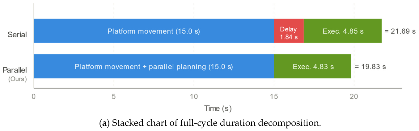
As illustrated in
Table 9 and
Figure 18a, the serial paradigm must wait for the completion of trajectory planning after braking, with a mandatory decision latency of
. In contrast, the parallel paradigm effectively eliminates this latency in all 80 tested scenarios (where
is satisfied throughout), enabling the system to trigger the pre-planned static execution trajectory with zero delay at the moment the platform stops at
s.
The proposed method reduces the mean full-cycle duration from to , achieving an overall operational efficiency improvement of 8.58%. This reduction (1.861 s) corresponds directly to the eliminated decision latency, while the duration of the static execution phase remains virtually unchanged (4.848 s vs. 4.827 s, a difference of only 0.4%). This suggests that, under the tested simulation conditions, the parallel planning mechanism does not compromise trajectory quality.
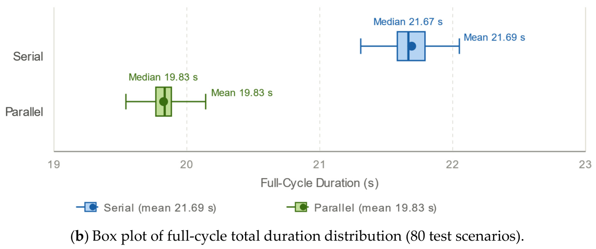
The box plot in
Figure 18b further demonstrates that the parallel paradigm exhibits significantly lower variance (standard deviation of 0.114 s vs. 0.163 s, a 30.1% reduction). This indicates more consistent task completion times across diverse operating conditions. Furthermore, the Interquartile Range (Q3−Q1) of the parallel paradigm (0.11 s) is much smaller than that of the serial paradigm (0.21 s). Within the obstacle-free simulation scope of this study, this enhanced predictability suggests potential benefits for multi-robot synchronization and coordination in flexible manufacturing environments; whether this advantage is preserved in environments with dynamic obstacles or cluttered workspaces remains a direction for future investigation.
This improvement holds particular practical significance in high-tempo flexible manufacturing scenarios involving repetitive task cycles, within the obstacle-free simulation scope of this study. As an illustrative estimate under the simulation conditions, for a production facility executing 500 grasping operations per shift in an obstacle-free environment, the proposed method would recover approximately 500 × 1.841 = 920 s of effective production time per shift compared to the serial paradigm. It should be noted that this estimate is derived from the obstacle-free simulation results and assumes ideal DT prediction conditions; actual throughput gains in real deployments—where dynamic obstacles, sensor noise, and model uncertainty are present—may differ and would require independent validation. Within the validated scope, when the optimization algorithm’s logic is complex and decision latency is non-negligible, the proposed full-cycle spatiotemporally coupled method indicates the potential to significantly suppress non-productive pauses during task execution in obstacle-free flexible manufacturing workflows.