Article

Integrating Adaptive Constraints with an Enhanced Metaheuristic for Zero-Latency Trajectory Planning in Robotic Manufacturing Processes

1
School of Economics and Management, Nanjing Tech University, Nanjing 211800, China
2
College of Management and Economics, Tianjin University, Tianjin 300072, China
3
College of Management, Tongling University, Tongling 244061, China
*
Author to whom correspondence should be addressed.
Processes 2026, 14(8), 1282; https://doi.org/10.3390/pr14081282
Submission received: 26 February 2026 / Revised: 8 April 2026 / Accepted: 14 April 2026 / Published: 17 April 2026
(This article belongs to the Section AI-Enabled Process Engineering)

Abstract

In flexible manufacturing systems, the composite mobile manipulator (CMM) is subject to nonlinear inertial disturbances arising from the dynamic coupling between the mobile platform and the robotic arm. These disturbances significantly impair positioning precision during grasping tasks. This paper addresses the dynamic decoupling of multi-body nonlinear inertial disturbances within CMM systems. Departing from the conventional “stop-then-plan” serial execution paradigm, we propose a full-cycle spatiotemporally coupled trajectory optimization method. The operation cycle is bifurcated into two synergistic stages: “dynamic calibration” and “static execution.” The dynamic calibration trajectory is pre-planned and executed synchronously during platform movement to actively compensate for inertial-induced pose deviations. Concurrently, the static execution trajectory is optimized and then triggered immediately upon platform standstill, ensuring a seamless and precise transition to the “Grasping Pose”. It is worth noting that the temporal characteristic central to this framework lies in the concurrent execution of static trajectory optimization and platform transit: by the time the platform reaches its destination, the pre-planned trajectory is already available for immediate triggering, achieving zero task-switching wait time at the planning layer. The term “zero-latency” here does not imply a fixed-cycle real-time response at the control layer, but rather the complete elimination of decision latency afforded by the parallel planning architecture. This framework eliminates computational latency, markedly enhancing operational efficiency. Key innovations include two novel constraints. First, the Adaptive Task-space Bounded Search Constraint (ATBSC) framework restricts optimization to a geometry-inspired search region, thereby enhancing search efficiency and ensuring controllable deviations. Second, the Multi-Rigid-Body Coupling Constraint (MRBCC) system explicitly models inertial transmission across motion phases to suppress pose fluctuations. The proposed framework is developed and validated within an obstacle-free workspace. In simulation-based validation on a UR10 6 degree-of-freedom manipulator model, experimental results indicate that ATBSC increases valid solution density to 84.7% and reduces average deviation by 72.8%. Furthermore, under the tested conditions, MRBCC mitigates end-effector position errors by 79.7–81.0% with a 97.5% constraint satisfaction rate. The improved Cuckoo Search algorithm (ICSA), serving as the solver component of the proposed framework, achieves an 11.9% lower fitness value and a 13.1% faster convergence rate compared to the standard Cuckoo Search algorithm in the tested scenarios, suggesting its effectiveness as a reliable solver for the constrained multi-objective trajectory optimisation problem.

1. Introduction

In flexible manufacturing systems, while traditional fixed-base industrial manipulators have been extensively studied, the composite mobile manipulator (CMM), which integrates a mobile platform with a robotic arm, has attracted increasing research attention in recent years [1]. Unlike fixed-base manipulators, CMMs experience complex dynamic interactions. The platform’s movement—including acceleration, deceleration, and turning—generates inertial forces that propagate through the kinematic chain. This process ultimately compromises end-effector positioning accuracy [2,3].
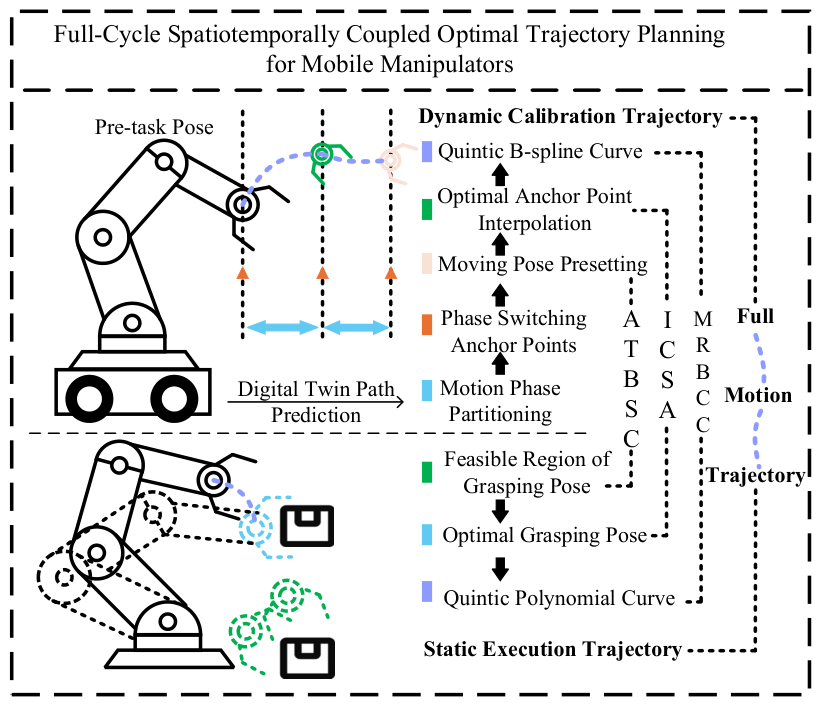
Departing from the prevailing “stop-then-plan” serial execution paradigm [4,5], this paper proposes a full-cycle spatiotemporally coupled trajectory planning method for CMMs. The operation cycle is bifurcated into two synergistic stages: “dynamic calibration” during platform transit and “static execution” during the grasping phase. The dynamic calibration trajectory is pre-computed and executed concurrently with platform movement. By leveraging Digital Twin (DT) predictions, this method proactively compensates for pose deviations induced by inertial forces during transit. The static execution trajectory is optimized during platform transit and triggered immediately upon platform standstill, eliminating post-braking trajectory planning latency. Within this methodological framework, this paper introduces two core technical innovations and adopts an improved algorithm as the trajectory solver:
First, we propose an Adaptive Task-space Bounded Search Constraint (ATBSC) method that adaptively constructs a bounded search region around a kinematically feasible reference configuration. Bounded initialization around inverse kinematics (IK) solutions is a common heuristic in motion planning. However, the novelty of ATBSC lies in its systematic integration into our spatiotemporally coupled framework. By introducing task-specific accuracy bounds for both motion phases, ATBSC simultaneously optimizes the calibration waypoints and the grasping pose search space. Simulation-based experimental results suggest that ATBSC reduces the joint space search volume to 0.12% of the original, increases valid solution density from 2.3% to 84.7%, boosts sampling efficiency by 36.9 times, and reduces average deviation by 72.8%.
Second, we propose a Multi-Rigid-Body Coupling Constraint (MRBCC) system based on temporal partition of the platform’s motion phases. By introducing phase-specific inertial coupling coefficients derived from the dynamic model, this system explicitly models the propagation of nonlinear inertial disturbances from the mobile platform to the manipulator joints. Integrated with the DT-driven pre-planning mechanism, MRBCC ensures that the manipulator converges precisely to the preset pose at the conclusion of platform transit, providing deterministic initial conditions for the static execution trajectory. Simulation-based experimental results suggest that MRBCC reduces end-effector position errors by 79.7%, 81.0%, and 79.8% during the acceleration, turning, and braking phases, respectively, with a constraint satisfaction rate of 97.5% under the tested conditions.
To meet the trajectory planning solver requirements of the proposed framework, an improved Cuckoo Search algorithm (ICSA) is introduced as the solver component. By incorporating the QUAntum Particle Swarm Optimization (QUAPSO) mechanism [6] and a Spray Mechanism, ICSA enhances the global exploration and local convergence performance of the standard Cuckoo Search (CS) algorithm. Experimental results demonstrate that, compared to the standard CS algorithm, ICSA reduces the fitness value by approximately 11.9% and increases convergence speed by 13.1%, and is capable of efficiently completing the pre-planning of the static grasping trajectory within the platform transit window.
The core conceptual framework of this study is schematically illustrated in Figure 1. The remainder of this paper is organized as follows. Section 2 reviews related work on mobile manipulator trajectory planning, manipulator disturbance compensation, and metaheuristic optimization for manipulator trajectory problems. Section 3 introduces the problem formulation for dynamic decoupling of nonlinear inertial disturbances and the full-cycle spatiotemporally coupled trajectory optimization methodology. Section 4 formulates the mathematical models, incorporating the ATBSC framework, the MRBCC system, and the multi-objective trajectory optimization model. Section 5 delineates the design principles of ICSA. Section 6 provides experimental validation and comparative analysis. Section 7 concludes the paper and discusses potential avenues for future research.

2. Related Work

This section reviews the literature most relevant to the present study along three thematic directions: mobile manipulator trajectory planning, manipulator disturbance compensation, and metaheuristic optimization for manipulator trajectory problems.

2.1. Mobile Manipulator Trajectory Planning

Mobile manipulator trajectory planning has been the subject of extensive research, with applications spanning industrial assembly, service robotics, and logistics [1]. Sandakalum and Ang [4] conducted a systematic review of motion planning methods for mobile manipulators, identifying the “stop-then-plan” serial paradigm as the dominant approach, wherein the robotic arm begins trajectory planning only after the mobile platform has reached a complete standstill. Fang et al. [7] proposed an iterative optimization framework for mobile manipulator trajectory planning in warehouse environments, employing dynamic programming and a genetic algorithm to optimize the arm trajectory and a modified A* algorithm to select the optimal stopping position, achieving significant reductions in total energy consumption under grasping accuracy constraints. However, all of the above studies operate within the “stop-then-plan” serial paradigm: they do not exploit platform transit time for concurrent trajectory computation, nor do they address the inertial coupling effects generated during platform movement.

2.2. Manipulator Disturbance Compensation

For fixed-base manipulators, disturbance rejection in trajectory planning has been addressed primarily through dynamic constraint formulation. Li et al. [8] employed Sequential Quadratic Programming to derive energy-optimal trajectories satisfying kinematic and dynamic constraints, achieving a 13.95% reduction in energy consumption compared to quintic polynomial trajectories. Xia et al. [9] proposed an enhanced velocity potential field algorithm that treats obstacle forces as dynamic disturbances within the planning framework, enabling collision-free navigation in surgical scenarios. However, these methods assume a stationary base: while dynamic constraint formulations provide a theoretical basis for handling manipulator disturbances, they tend to treat disturbances as static or slowly varying external inputs. Disturbances from the mobile platform exhibit non-smooth, time-varying, and multi-phase coupling characteristics. Existing methods lack explicit modeling of the dynamic inertial coupling generated during acceleration, turning, and braking. Consequently, they cannot proactively compensate for the shifting inertial forces inherent in CMM operation.
For mobile manipulators, compensating for platform-induced inertial disturbances has attracted increasing research attention [2,3]. Feng et al. [2] investigated the effect of chassis suspension deformation on mobile manipulator end-effector accuracy, using multi-sensor fusion to measure and compensate for pose changes during platform transit. Zhou et al. [3] explicitly encoded cross-body inertial coupling through an off-diagonal inertia matrix, establishing a coupled dynamic model for a collaborative industrial mobile manipulator with experimental validation of the platform-arm coupling dynamics, which also provides the theoretical foundation for the inertial coupling coefficient derivation in this paper.
In the domain of space robotics, base-motion-induced disturbances on the manipulator have similarly been studied. Zhang et al. [10] proposed trajectory planning to minimize base disturbance for a redundant space robot using an improved quantum particle swarm optimization algorithm, and Xiao [11] addressed non-holonomic path planning for space robots under jerk constraints. Although the coupling mechanisms of ground-based CMMs and space robots differ, both require explicit modeling of base-arm interactions in trajectory planning—a challenge that the MRBCC method proposed in this paper addresses specifically for the CMM setting.

2.3. Metaheuristic Optimization for Manipulator Trajectory Problems

Metaheuristic algorithms have become important solvers for robot trajectory planning owing to their ability to handle non-convex, multi-objective problems with non-smooth constraints.
A substantial body of work has applied metaheuristic algorithms to fixed-base manipulator trajectory planning. Chen et al. [12] demonstrated the effectiveness of quantum-behaved particle swarm optimization combined with quintic B-spline curves for time-energy-jerk optimal trajectory planning of high-speed parallel manipulators. Lopez-Franco et al. [13] proposed a general metaheuristic framework for multi-joint manipulator trajectory tracking, demonstrating its superiority over Jacobian-based methods in handling non-convex, high-dimensional search spaces. The QUAPSO algorithm of Flori et al. [6] incorporates quantum superposition principles into the particle swarm framework, exhibiting strong performance on complex multi-modal optimization problems.
Metaheuristic methods have also been applied to mobile manipulator trajectory planning. Hussein et al. [14] proposed a hybrid integral sliding mode and fuzzy logic control framework for omnidirectional mobile robots, employing a modified elephant herding optimization algorithm for trajectory tracking under dynamic disturbance conditions, validating the feasibility of metaheuristic methods for mobile robot trajectory planning.
The original CS algorithm proposed by Yang and Deb [15], combining Lévy flight for global exploration with an alien-egg replacement mechanism for local convergence, has been applied to various trajectory optimization problems. Several improvements have been proposed: Walton et al. [16] enhanced population diversity through an information exchange mechanism; Huang et al. [17] integrated differential evolution strategies to improve local search precision; Mareli and Twala [18] introduced an adaptive step-length adjustment strategy to balance exploration and exploitation. However, these improvements each focus on a single mechanism, and the alien-egg replacement process continues to rely on a simple random replacement strategy lacking directional guidance. More fundamentally, these modifications are designed for smooth, continuous constraint structures and are therefore not well suited to solving the dynamic calibration trajectory under the MRBCC framework.

3. Problem Formulation: Dynamic Decoupling of Nonlinear Inertial Disturbances

For material handling tasks within flexible workshops, the operational process of a CMM is partitioned into three core phases:
(1)
Moving Phase: The mobile platform moves to the grasping task site under an unload condition or performs transport tasks under a load condition. During this process, the robotic arm maintains a stable “Moving Pose” θ t j m to ensure safety and energy efficiency. This phase concludes when the mobile platform reaches the grasping task site and comes to a complete standstill.
(2)
Grasping Phase: Upon the platform’s arrival and standstill at the task site, the robotic arm’s end-effector must move precisely to the target coordinates of the “Grasping Pose” ( x t a r g e t g , y t a r g e t g , z t a r g e t g ) to execute material grasping, where the joint angles must satisfy accuracy constraints to achieve high-precision manipulation.
(3)
Placement Phase: After the robot reaches the designated placement site and stops, the robotic arm transitions from the “Moving Pose” to the “Placement Pose” to complete the task. This phase follows the same motion strategy as the Grasping Phase.
As the robotic arm base is mounted directly on the mobile platform, the platform’s motion state during the Moving Phase dictates the nonlinear inertial forces exerted on the robotic arm joints. We discretize the movement process of the mobile platform within the Moving Phase into the following 4 distinct phases:
(1)
Acceleration Phase (ma): Defined by time nodes { t 1 m a , t 2 m a , , t a m a } . The linear acceleration generated by the platform propagates through the base to the joints, characterized by a coupling coefficient k j m a .
(2)
Constant-Speed Phase (ms): Defined by time nodes { t 1 m s , t 2 m s , , t b m s } . In this phase, inertial disturbances exhibit a natural attenuation trend.
(3)
Turning Phase (mt): Defined by time nodes { t 1 m t , t 2 m t , , t c m t } . Centrifugal forces resulting from the platform’s turning exert lateral disturbances on the joints, characterized by a coupling coefficient k j m t .
(4)
Braking Phase (mb): Defined by time nodes { t 1 m b , t 2 m b , , t e m b } . Negative acceleration produces inertial impacts that may induce pose shifts, characterized by a coupling coefficient k j m b .
This study focuses on the trajectory optimization of the mobile manipulator from its initial position to its standstill and subsequent task execution at the grasping site (Moving Phase + Grasping Phase), with the goal of deriving the optimal motion trajectory mg. Departing from the “stop-then-plan” serial planning paradigm [4,5], we propose a full-cycle spatiotemporally coupled trajectory optimization method. The core concept involves bifurcating the trajectory into two synergistic stages: “dynamic calibration” during the Moving Phase and “static execution” during the Grasping Phase. Computational latency is eliminated through temporal parallel pre-planning, while inertial disturbances are suppressed through spatial proactive compensation.
The framework comprises two synergistic trajectory components. The dynamic calibration trajectory is planned before the initiation of the Moving Phase and executed concurrently with the platform’s transit. The target “Moving Pose” is first determined via the ATBSC framework, after which DT technology simulates the platform’s trajectory to predict inertial coupling effects across all motion phases. Intermediate interpolation points are established at phase-switching moments as time anchors, with their positions serving as decision variables for the ICSA; the trajectory is then synthesized using quintic B-spline curves [12] to satisfy the MRBCC, ensuring that the end-effector pose precisely converges to the preset “Moving Pose” at the conclusion of the Moving Phase. The static execution trajectory, in turn, is optimized during platform transit and triggered immediately upon standstill, taking the terminal pose of the dynamic calibration trajectory as its starting configuration and the ATBSC-derived “Grasping Pose” as its target. These two trajectory segments are seamlessly integrated into the full motion trajectory, with the Moving Phase conclusion serving simultaneously as the Grasping Phase initiation.
To ensure robust execution in physical deployments where inertial disturbances may deviate from DT predictions, it is recommended that pose sensors—such as an inertial measurement unit, torque sensors, or a vision system—be configured at the end-effector to provide closed-loop verification of the terminal convergence of the dynamic calibration trajectory to the preset “Moving Pose.”

4. Mathematical Modeling

4.1. Mathematical Description of the Full-Cycle Spatiotemporally Coupled Trajectory Optimization Framework

To characterize the spatiotemporal evolution of the CMM over the complete operational cycle, we define the full-cycle trajectory mg as the composite of the dynamic calibration phase and the static execution phase.

4.1.1. Full-Cycle Time Domain Partitioning

We define the initiation of the operational cycle—the moment the mobile platform begins its transit based on task requirements—as t = 0 , and the moment the platform reaches a complete standstill (the task switching point) as t s t o p . The full-cycle time domain T is bifurcated into two complementary subsets as shown in Equation (1):
T = T c a l T e x e , T c a l T e x e =  
where the dynamic calibration time domain T c a l = { t 0 t t s t o p } corresponds to the platform’s transit process, and the static execution time domain T e x e = { t t s t o p < t t e n d } corresponds to the grasping task execution after the platform has halted.

4.1.2. Temporal Coupling: Parallel Planning and Latency Elimination

Let t s o l v e denote the computational time required to solve for the static execution trajectory. The proposed parallel paradigm requires the static execution trajectory to be optimized concurrently during t [ 0 , t s t o p ] . The computational latency Δ t d e l a y is formulated in Equation (2):
Δ t d e l a y = m a x ( 0 , t s o l v e T m o v e ) ,     T m o v e = t s t o p
This formulation indicates that if the trajectory optimization concludes before the platform stops ( t s o l v e < t s t o p ), the computational latency is eliminated (reduced to 0). In this paper, ‘real-time’ specifically means that trajectory optimization occurs in parallel with platform transit. By avoiding post-standstill delays, the system responds at the moment of task transition with zero computational latency. This is distinct from fixed-cycle real-time response at the control layer. Conversely, in the conventional “stop-then-plan” serial paradigm, trajectory optimization is only triggered after t   =   t s t o p , yielding a latency of t s o l v e   >   0 .

4.2. ATBSC Framework

4.2.1. Reference Configuration and Bounded Search Region

Given a target end-effector pose T t a r g e t , a reference joint configuration θ r e f is obtained by solving the IK as in Equation (3).
θ r e f = I K ( T t a r g e t )
where θ r e f Q represents a kinematically feasible joint configuration corresponding to the target pose. This reference configuration serves as the center of the bounded search region constructed in the following definition.
Definition 1.
(Accuracy-Bounded Search Region). To construct a computationally tractable search domain around the reference configuration, we define a component-wise bounded region in joint space using an L norm. Given a reference configuration θ r e f Q and per-joint accuracy bounds ε j , the accuracy-bounded search region is defined as in Equation (4).
N ε ( θ r e f ) = { θ Q : | θ j θ j r e f | ε j ,       j = 1 , , n }
The deviation variables must satisfy ε j ε j m a x , where ε j m a x denotes the maximum permissible joint error threshold. The ATBSC framework constrains the optimization search space of the trajectory endpoint joint angles within the intersection defined in Equation (5).
S A T B S C = N ε ( θ r e f ) Q a d m i s s i b l e
where Q a d m i s s i b l e represents the kinematically admissible region satisfying all joint limit constraints.

4.2.2. ATBSC Implementation Strategy

The ATBSC method consists of two synergistic components: the “Grasping Pose Accuracy-Bounded Search Region” and the “Moving Pose Bounded Search Region”, corresponding to the end and start configurations of the static execution trajectory, respectively.
(1)
Grasping Pose Accuracy-Bounded Search Region
The “Grasping Phase” demands extremely high positioning accuracy to ensure precise manipulation. The ATBSC framework constructs an accuracy-bounded search region around a kinematically solved reference configuration. First, based on the target position ( x t a r g e t g ( t ) , y t a r g e t g ( t ) , z t a r g e t g ( t ) ) , the end-effector position P e g is determined, and a feasible “Grasping Pose” is obtained via IK as the reference configuration θ j g , r e f . Subsequently, the accuracy deviation variable ε j g for each joint is introduced to define the ATBSC optimization domain for the “Grasping Pose”. The Grasping Pose Accuracy-Bounded Search Region is defined as shown in Equation (6).
S A T B S C g = { θ : θ j g , r e f ε j g θ j θ j g , r e f + ε j g , j = 1 , , n } Q a d m i s s i b l e
where θ j g , r e f represents the reference joint angle configuration of the j -th joint obtained from IK, and ε j g denotes the maximum allowable deviation for joint j during the Grasping Phase. The bounded search space S A T B S C g significantly reduces optimization complexity while ensuring solution quality. The accuracy boundaries prevent discontinuous jumps in joint positions, thereby guaranteeing trajectory smoothness.
(2)
Moving Pose Bounded Search Region
The “Moving Pose” serves as the starting point of the static execution trajectory. When the robot is in the “Moving Phase”, the primary objective is workpiece transportation, where accuracy requirements are relatively relaxed. The configuration of the preset “Moving Pose” follows the principle of selecting any posture that ensures the mobile manipulator maintains stability without tipping over during platform movement, i.e., a stable pose configuration.
First, a preset “Moving Pose” θ j m , r e f is determined based on stability requirements and physical constraints. Subsequently, the maximum allowable deviation ε j m for each joint is introduced to define the ATBSC optimization domain for the “Moving Pose”. The Moving Pose Bounded Search Region is defined as shown in Equation (7).
S A T B S C m = { θ : θ j m , r e f ε j m θ j θ j m , r e f + ε j m , j = 1 , , n } Q a d m i s s i b l e
where θ j m , r e f represents the reference joint angle of the j -th joint in the preset “Moving Pose”, and ε j m denotes the maximum allowable deviation for joint j during the Moving Phase. Since accuracy requirements during the “Moving Phase” are relatively relaxed compared to the “Grasping Phase”, the deviation bounds ε j m are set more loosely than the grasping accuracy deviation ε j g . The joint angle values within this domain must satisfy transportation task requirements while complying with physical constraint limits.
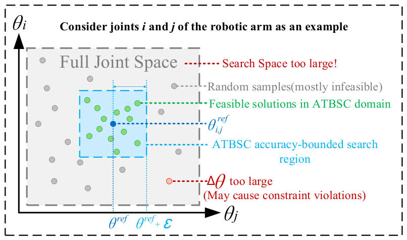
The geometric intuition of ATBSC is illustrated in Figure 2.
Note that this paper focuses on trajectory optimization in obstacle-free environments to isolate the individual effects of the ATBSC and MRBCC methods. By constructing a geometry-inspired bounded search space, the ATBSC framework transforms the conventional pose-setting problem into a structured and controllable optimization problem. Specifically, it determines the optimal interpolation positions for intermediate waypoints in the dynamic calibration trajectory and constructs the feasible search space for the optimal “Grasping Pose” in the static execution trajectory, providing geometrically constrained configurations for subsequent trajectory generation.
In practical deployment, the accuracy bounds ε j require task-specific calibration. The representative pose set should cover the spatial diversity of the deployment workspace: in practice, we recommend sampling target grasping positions that span the reachable workspace at a minimum of 5–10 uniformly distributed locations, including poses near the workspace boundary where joint configurations are more varied, and at least one pose near each of the primary task locations anticipated in the deployment. For each sampled target, the reference configuration is obtained by executing IK; if multiple IK solutions exist, the one closest to the nominal “Moving Pose” θ m , ref in joint space should be selected to maintain consistency with the ATBSC bounded search region. The maximum joint deviation observed across all sampled reference configurations defines the lower bound for ε j : the final ε j is set to this maximum deviation plus a small safety margin (e.g., 0.5° to 1°) to accommodate unseen poses within the deployment workspace. As ε j increases, the search space expands and feasibility improves, but end-effector positioning error also increases—the ε -sensitivity analysis in Section 6.3.1 (3) shows that ε =   3 ° represents the optimal trade-off for the UR10 configuration studied, and can serve as a practical starting point for similar industrial manipulators. The bound for the Moving Phase is typically set more loosely than that for the Grasping Phase, as the precision requirements during platform transit are less stringent than those for the grasping operation itself. Both bounds must satisfy the physical joint constraints to ensure that the bounded search region remains within the kinematically admissible space Q a d m i s s i b l e .
However, ATBSC alone cannot fully resolve the dynamic inertial disturbance problem arising from platform movement. Therefore, the MRBCC framework is introduced in the following section to complement this limitation.

4.3. MRBCC Framework for Inertial Disturbance Mitigation

4.3.1. DT-Driven Dynamic Pose Calibration Strategy

To address the nonlinear inertial disturbance problem arising from the mobile platform’s movement during the operation of the CMM, this paper proposes a DT-driven dynamic calibration trajectory pre-planning mechanism:
Prior to the initiation of the Moving Phase, the DT simulates and predicts the future motion phases of the mobile platform based on the input global path planning scheme, determining when the platform will be in which motion phase. Based on the predicted motion phases and their switching moments (time anchors), a dynamic calibration trajectory is pre-planned for the manipulator. When the platform undergoes dynamic processes such as acceleration, constant-speed cruising, turning, and braking, the robotic arm does not remain absolutely stationary but instead executes the pre-planned dynamic calibration trajectory to counteract pose uncertainty induced by inertial force transmission.
This DT-driven strategy provides two complementary guarantees for the full-cycle framework. During the Moving Phase, the manipulator autonomously executes the pre-planned dynamic calibration trajectory concurrently with platform transit (in the planning-layer parallel sense defined in Section 4.1.2) to remain in the vicinity of the preset “Moving Pose”, preventing severe pose deviation caused by excessive coupling effects that could otherwise lead to joint torque saturation or manipulator instability. At the conclusion of the Moving Phase, the manipulator pose is precisely locked at the preset “Moving Pose”, thereby providing the deterministic initial condition that enables the static execution trajectory to be optimized and triggered without delay.
The DT employed in this framework is grounded in the coupled rigid-body dynamics of the CMM system, governed by the standard equation of motion as shown in Equation (8) [3].
M ( q ) q ¨ + C ( q , q ˙ ) q ˙ + G ( q ) = τ + τ ext
where the off-diagonal inertia matrix M ( q ) encodes the dynamic coupling between the mobile platform and the robotic arm [3]. The DT constructs a virtual replica of the mobile platform and models its motion as a rigid-body state transition sequence spanning four motion phases (acceleration, constant-speed, turning, and braking). The DT has the following explicit input-output structure:
Input: The global path planning scheme specifying the mobile platform’s trajectory from its initial position to the grasping site. In the simulation-based validation presented in this paper, this path is generated in an obstacle-free environment according to the randomization principles described in Table 1.
Output: The motion phase sequence and phase-switching moments (time anchors) of the platform motion cycle, together with the characteristic accelerations of each phase—specifically, the linear accelerations of the acceleration and braking phases ( a p m a and a p m b ) and the centripetal acceleration of the turning phase ( a c m t ). These outputs serve two coupled functions within the framework. First, they define the time anchors used to establish the intermediate interpolation points of the dynamic calibration trajectory. Second, and more critically, they supply the platform acceleration input a p for the derivation of the inertial coupling coefficients k j ( ) in Section 4.3.2, thereby establishing a direct chain: the DT predicts the characteristic accelerations of each phase, and the coupled dynamic equations map these accelerations to the joint-level constraint bounds within the MRBCC system.
In the simulation-based validation presented below, the platform path is assumed to be known a priori before trajectory optimization begins, which is equivalent to a DT output with zero prediction error under known-path conditions. This renders the computational overhead of DT prediction negligible: the phase-switching moments and characteristic accelerations are analytically determined from the path planning scheme before platform initiation, requiring no iterative computation and introducing no additional latency into the full-cycle framework.
In physical deployment, the DT requires an accurate rigid-body kinematic model of the CMM system as its underlying simulation engine, including the Denavit–Hartenberg (DH) parameters and link inertial properties (mass and inertia tensors) of the robotic arm, which are typically available from the manufacturer’s datasheet. The motion path data of the mobile platform is generally obtained from the path planning solution generated by the system based on its material handling task requirements, thereby providing sufficiently accurate real-time estimates of the phase-switching moments and characteristic accelerations ( a p m a , a p m b , a c m t ) for the MRBCC system. It should be noted that this paper assumes zero discrepancy between DT predictions and actual motion data; accordingly, the propagation of DT prediction errors to trajectory quality is left as a direction for future work, as discussed in Section 7.

4.3.2. Moving Phase Decomposition and Coupling Modeling

Based on the predictions from the DT system, the motion cycle of the mobile platform (Moving Phase) is discretized according to the four phases mentioned previously.
To quantify the disturbance intensity exerted by the platform’s motion states on each joint of the manipulator, we introduce the inertial coupling coefficient k j ( ) , where the superscript ( ) { m a , m t , m b } corresponds to the three motion phases with significant inertial disturbances: acceleration, turning, and braking, respectively. The physical interpretation of k j ( ) is the equivalent angular acceleration constraint boundary induced at the j -th joint per unit characteristic acceleration (linear acceleration or centripetal acceleration) of the mobile platform. Its numerical value is determined by the geometric structure of the manipulator at the reference configuration and the link mass distribution. A larger k j ( ) indicates higher sensitivity of the joint to platform movement.
The coefficients k j ( ) are derived directly from the coupled equation of motion established in Section 4.3.1. When the mobile platform undergoes a linear acceleration a p (predicted by the DT) in the world frame, the manipulator base is subjected to an equivalent pseudo-force. The term τ e x t d ( a p , q ) in the equation of motion represents the generalized inertial disturbance torque induced by the platform acceleration (as distinct from external contact forces) [3]. Here, q R n denotes the joint configuration vector and n is the total number of joints. Isolating the disturbance term from the equation of motion, the generalized inertial disturbance torque at joint j can be expressed through the manipulator’s positional Jacobian matrix and link masses as shown in Equation (9).
d j ( a p , q ) = i = j n m i J p , i T ( q ) a p
where d j is the disturbance torque at joint j ; m i is the mass of the i -th link; J p , i ( q ) R 3 × n is the positional Jacobian matrix that maps joint velocities to the linear velocity of the center of mass of the i -th link; and a p R 3 is the platform acceleration vector predicted by the DT (defined in Section 4.3.1). The equivalent angular acceleration disturbance at joint j is given by Equation (10).
Δ θ j ¨ = M j 1 ( q ) d j ( a p , q )
where Δ θ j ¨ denotes the equivalent angular acceleration disturbance at joint j , and M j 1 ( q ) is the j -th row of the inverse joint inertia matrix M 1 ( q ) . Within the neighborhood of the reference configuration θ m , ref , M ( q ) can be approximated as the constant M ( θ m , ref ) , with an approximation error of order O ( ε j m ) . Since ATBSC guarantees that ε j m is a controllably small quantity (Section 4.2), this linearization is self-consistently justified. Consequently, the above relation simplifies to Δ θ j ¨ k j ( ) a p , where k j ( ) is computed as shown in Equation (11).
k j ( ) = M j 1 ( θ m , ref ) i = j n m i J p , i T ( θ m , ref )
This expression indicates that k j ( ) can be analytically estimated from the known DH parameters of the manipulator, the link inertial properties { m i , I i } , and the reference configuration θ m , r e f , without requiring physical experiments. This expression clarifies the dependencies of k j ( ) . It depends on the payload (via link mass m i ) and the reference configuration θ m , r e f , but remains independent of platform velocity. Instead, velocity influences MRBCCs through the DT-predicted characteristic accelerations, a p m a and a c m t . Although k j ( ) formally depends on q through M j 1 and J p , i T , within the MRBCC framework it is evaluated at the fixed reference configuration θ m , r e f . This is self-consistently justified because ATBSC (Section 4.2) constrains the dynamic calibration trajectory to satisfy | θ j θ j m , r e f | ε j m throughout the entire Moving Phase, thereby keeping the linearization error of the first-order Taylor expansion M ( q ) M ( θ m , r e f ) + O ( ε j m ) bounded and controllable. When the manipulator operates under no-load conditions, k j ( ) is computed using the unloaded link mass values. For loaded operations, k j ( ) needs only to be recomputed with the updated link inertial parameters prior to trajectory planning—a straightforward application of the same analytical procedure that requires no additional identification experiments.
The active calibration constraints and dynamic transmission models for each phase are formulated as follows:
(1)
Acceleration Phase (ma): During this phase, the platform’s linear acceleration propagates through the base to the joints, generating inertial force disturbances. The combined acceleration of the manipulator should be the sum of the inertial disturbance acceleration and its own active acceleration. The calibration trajectory must satisfy the following constraints:
θ j m a ( t a m a ) θ j m , r e f ε j m
θ ˙ j m a ( t a m a ) = 0
θ ¨ j m a ( t a m a ) = 0
| k j m a · a p m a + θ ¨ j m a ( t ) | θ ¨ j , m a x
where a p m a denotes the platform’s linear acceleration, and θ ¨ j , m a x presents the joint-specific maximum angular acceleration of joint j .
(2)
Constant-Speed Phase (ms): During the constant-speed phase, the platform acceleration is 0, and inertial disturbances exhibit a natural attenuation trend as shown in Equations (16) and (17). Beyond basic kinematic and dynamic constraints, the calibration trajectory in this phase only needs to satisfy the ε j m deviation constraint as specified in Equation (16).
θ j m s ( t b m s ) θ j m , r e f ε j m
0 θ ¨ j m s ( t b m s ) θ ¨ j m s ( t 1 m s )
(3)
Turning Phase (mt): Centrifugal forces generated by platform turning constitute another factor inducing end-effector instability. Based on the centripetal acceleration a c m t predicted by the DT, we explicitly model the lateral disturbance transmission process through the coupling coefficient k j m t . The purpose of the calibration trajectory in this phase is to compensate for pose drift caused by centrifugal forces. Beyond basic kinematic and dynamic constraints, the calibration trajectory should satisfy the constraints specified in Equations (18) and (19).
| k j m t · a c m t + θ ¨ j m t ( t ) | θ ¨ j , m a x
θ j m t ( t c m t ) θ j m , r e f ε j m
(4)
Braking Phase (mb): As the terminal segment of the Moving Phase, calibration during braking is critically important. The terminal conditions determine the initial quality of the subsequent “Grasping Phase” (as shown in Equations (20) and (21)). The braking coupling coefficient k j m b quantifies the disturbance induced by deceleration. Additionally, the calibration trajectory in this phase must satisfy the terminal zeroing constraints for velocity and acceleration as specified in Equations (22) and (23), which minimizes trajectory-switching-induced oscillations when the mobile platform comes to a halt and triggers the static execution trajectory, thereby enhancing the stability of the initial position for the “Grasping Phase”.
| k j m b a p m b + θ ¨ j m b ( t ) | θ ¨ j , m a x
θ j m b ( t e m b ) = θ j m , r e f
θ ˙ j m b ( t e m b ) = 0
θ ¨ j m b ( t e m b ) = 0
Based on the constraints for each motion phase, the manipulator calibrates the “Moving Pose” to within the ε j m deviation constraint range at the conclusion of each phase during platform movement, following the pre-planned trajectory. Among these, θ j m a ( t a m a ) , θ j m s ( t b m s ) , and θ j m t ( t c m t ) each represent a set of intermediate interpolation points for the dynamic calibration trajectory, all of which must lie within the ATBSC domain of θ j m , r e f ; while θ j m b ( t e m b ) represents the trajectory endpoint, i.e., the preset “Moving Pose” θ j m , r e f . The MRBCC framework establishes an explicit mapping relationship between the mobile platform’s motion states and the manipulator joint responses through motion phase partitioning and inertial coupling coefficient modeling, thereby addressing the problem of “how to maintain end-effector stability during platform movement”. Together, ATBSC and MRBCC constitute the constraint system of the full-cycle spatiotemporally coupled framework: the former constrains the geometric feasibility of trajectory endpoints, while the latter constrains the dynamic stability throughout the entire trajectory. The two are coupled through the junction point between the dynamic calibration trajectory and the static execution trajectory (i.e., the preset “Moving Pose” θ j m , r e f ).
In practical deployment, the inertial coupling coefficients k j ( ) can be analytically computed via Equation (11), evaluated at the reference configuration θ m , ref under the current payload conditions. For deployment scenarios involving different manipulators, different payloads, or different reference configurations, the coefficients should be recomputed using the corresponding DH parameters and link inertial properties from the manufacturer’s specifications. Note that k j ( ) is payload-dependent: for operations involving known payloads, the equivalent end-link mass should be updated accordingly before recomputing the coefficients.

4.4. Multi-Objective Optimization Model

The dynamic calibration trajectory and static execution trajectory of the CMM adopt a unified multi-objective optimization model. The optimization objectives integrate three performance metrics: time efficiency F m g T , energy consumption F m g E , and trajectory smoothness F m g S . Here, Q j i m g ( t ) denotes the joint angle of the j -th joint on the i -th sub-trajectory segment at time t , while Q ˙ j i m g ( t ) , Q ¨ j i m g ( t ) , and Q j i m g ( t ) represent the corresponding angular velocity, angular acceleration, and angular jerk, respectively. h i m g = t i + 1 m g t i m g denotes the time interval of the i -th sub-trajectory segment.
m i n F m g = ω m g 1 F m g T + ω m g 2 F m g E + ω m g 3 F m g S
ω m g 1 + ω m g 2 + ω m g 3 = 1
F m g T = i = 1 m 1 h i m g
F m g E = j = 1 n i = 1 m 1 [ t i m g t i + 1 m g ( α m g ( Q ˙ j i m g ( t ) ) 2 + β m g ( Q ¨ j i m g ( t ) ) 2 ) d t ]
F m g S = j = 1 n i = 1 m 1 [ t i m g t i + 1 m g ( Q j i m g ( t ) ) 2 d t ]
s . t .                   Q m i n m g Q j i m g ( t ) Q m a x m g
| Q ˙ j i m g ( t ) | V m a x m g
| Q ¨ j i m g ( t ) | A m a x m g
| Q j i m g ( t ) | J m a x m g
| τ j ( t ) | τ j , m a x
where the energy consumption objective F m g E is the squared integral of angular velocity and angular acceleration, with α m g and β m g being the energy consumption weighting coefficients for the angular velocity term and angular acceleration term, respectively; the smoothness objective F m g S is the squared integral of angular jerk. In addition to the multiple constraints presented previously, Equations (29)–(32) represent the angular position, angular velocity, angular acceleration, and angular jerk constraints that the manipulator motion trajectory based on quintic polynomial curves must satisfy. The output torque of joint motors is limited by physical hardware; exceeding the rated torque will cause motor overload or even damage. Therefore, we also introduce the maximum joint torque constraint for the j -th joint of the manipulator as shown in Equation (33), where τ j ( t ) denotes the driving torque of the j -th joint at time t , and τ j , m a x is the maximum allowable torque for that joint.

5. Optimal Trajectory Optimization Algorithm

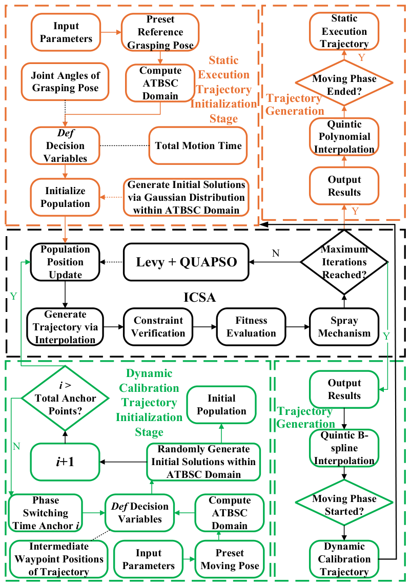
The flowchart of the trajectory optimization algorithm for mobile manipulators based on the full-cycle spatiotemporally coupled framework is illustrated in Figure 3. The process can be broadly divided into three stages: the initialization stage for dynamic calibration trajectory optimization and static execution trajectory optimization, the ICSA optimal solution stage, and the trajectory parameterization stage.

5.1. Fundamental Principles of the Algorithm

The CS algorithm is a metaheuristic optimization technique inspired by the brood parasitism behavior of cuckoos [15]. The algorithm primarily employs two mechanisms: Lévy flight for global exploration and alien egg replacement for local convergence of solutions. During the search process, candidate solutions are treated as “eggs”. The algorithm iteratively searches for the global optimum by simulating two behaviors: cuckoos laying eggs in host nests, and host birds identifying and discarding alien eggs.
The selection of a population-based metaheuristic algorithm as the solver for this framework is driven by two structural characteristics of the problem. First, the MRBCC phase-switching constraints are non-smooth and non-convex. As the platform transitions between motion phases, the constraints change discontinuously. This renders gradient-based solvers, such as Sequential Quadratic Programming, inapplicable without complex reformulation or relaxation. Second, the full-cycle parallel planning paradigm imposes a strict bounded-time requirement: the static grasping trajectory must be fully optimized within the platform transit window T move (see Section 6.3.3). Population-based metaheuristic algorithms always terminate within a fixed number of iterations and always return the best feasible solution found, providing fully predictable and bounded computation time. Exact solvers cannot provide such guarantees on non-convex problems; occasional failure to converge within T move would invalidate the entire parallel planning framework. These two properties jointly make population-based metaheuristic algorithms a suitable solver class for this problem.
This bounded-time reliability directly underpins the planning-layer “zero-latency” property of the proposed framework (in the sense defined in Section 4.1.2—the completion of trajectory optimization within the platform transit window, not a fixed-cycle control-layer real-time response): since ICSA always completes within a fixed number of iterations, the trajectory solving time tsolve is guaranteed to be bounded, enabling the parallel planning paradigm to achieve zero decision latency by design.
Within this framework, a key practical constraint faced by ICSA is that “the static execution trajectory must be fully solved before the mobile platform completes its transit”, i.e., t solve T move . For scenarios with shorter transit times, the solver budget needs to be re-evaluated. Feasible approaches include, but are not limited to, reducing the population size N while accepting a slight degradation in solution quality. The bounded initialization provided by ATBSC is particularly beneficial in this context, as it compresses the effective search space, directly reducing the computational overhead per iteration of ICSA.

5.2. Integration of the QUAPSO Mechanism

The population position update in the standard CS algorithm relies solely on the random step length of Lévy flight, where particles move from their current positions along a single random direction. This approach neither effectively utilizes the historical best information of the population nor achieves a dynamic balance between global exploration and local exploitation. The Quantum Superposition Principle offers a novel perspective to address this limitation: in quantum mechanics, a particle can simultaneously exist in a superposition of multiple possible states before being observed [6]. Introducing this concept into optimization algorithms means that candidate solutions are no longer confined to deterministic single-point updates but exist as probability distributions across multiple potential positions, collapsing to specific positions through “observation” operations (i.e., sampling). This mechanism endows the algorithm with two key capabilities: (1) particles can escape local optima traps with a certain probability through the quantum tunneling effect; and (2) by integrating the mean best position information of the population, it provides directional guidance for the search process toward globally optimal regions.
To address the insufficient local convergence capability and susceptibility to premature convergence of the standard CS algorithm, we introduce the QUAPSO algorithm mechanism [6] based on quantum superposition principles. By combining the characteristics of quantum wave functions with the random step length of Lévy flight, the updated particle position formula is given in Equation (34):
x i d , ( t + 1 ) = P i d , ( t + 1 ) ± β ( m B e s t i d X i d , t ± α · L e v y ( λ ) ) l n ( 1 u γ )
where x i d , ( t + 1 ) denotes the updated position of the i -th particle in the d -th dimension; P i d , ( t + 1 ) represents the individual historical best position of that particle; α is the Lévy flight step length scaling factor; L e v y ( λ ) is the random step length following a Lévy distribution with λ being the distribution index; u γ ( 0,1 ) is a uniformly distributed random number; and β is the contraction-expansion coefficient.
The physical significance of the key terms warrants explicit discussion. The term ln ( 1 u γ ) originates from the probability density function of a particle in a quantum potential well model [6,19]. Its physical significance lies in the following: when u γ approaches 0, this term tends toward infinity, enabling particles to achieve long-distance jumps with small probability (quantum tunneling effect), thereby effectively escaping local optima; when u γ approaches 1, this term tends toward 0, and particles conduct fine-grained search within the current optimal region. The term m B e s t i d , as the mean of all particles’ historical best positions, represents the collective search experience of the population. The difference ( m B e s t i d X i d , t ) between this mean best position and the current position X i d , t defines a search direction pointing toward high-quality solution regions, guiding particles to converge toward globally optimal areas. This hybrid update strategy, combining quantum probabilistic sampling with Lévy flight, balances global exploration capability and local convergence precision within a single update rule. The adaptive parameter γ is defined as shown in Equation (35):
  γ ( i t e r a t i o n ) = γ i n i t i a l · e k · i t e r a t i o n M
where γ i n i t i a l is the initial value of γ , k is the decay rate constant, M is the maximum number of iterations, and i t e r a t i o n is the current iteration count. In the early stages of the search, a larger γ value enhances global exploration capability; in the later stages, a smaller γ value helps improve local search precision. This mechanism effectively balances the algorithm’s global exploration and local convergence performance.

5.3. Integration of the Spray Mechanism

The alien egg replacement mechanism in the standard CS algorithm adopts a simple random replacement strategy: when the host bird discovers an alien egg with probability P a , the solution is replaced by a completely random new solution. This mechanism suffers from two critical deficiencies: (1) the newly generated solutions are entirely unrelated to the population’s historical best information and global best information, resulting in a lack of directional guidance for the search; (2) in the later stages of iteration, the algorithm still performs large-scale random jumps within the entire solution space, failing to effectively focus on high-quality solution regions, which severely impacts convergence efficiency. To address these issues, we draw inspiration from fluid mechanics and propose a directional replacement mechanism named Spray Mechanism based on spray droplet dynamics. This mechanism assumes that the initial population’s positions and velocities follow Gaussian distributions [20], as shown in Equation (36).
{ x i ~ N ( μ x , σ x 2 ) y i ~ N ( μ y , σ y 2 ) x i = min ( max ( x i , x 1 ) , x 2 ) y i = min ( max ( y i , y 1 ) , y 2 )
where ( x i , y i ) denotes the initial position of the i -th droplet, ( μ x , μ y ) and ( σ x 2 , σ y 2 ) represent the mean and variance of the position distribution, respectively, and ( x i , x 1 ) and ( y i , y 1 ) define the boundary ranges of the search space.
Under aerodynamic drag, the position of the i -th droplet evolves as shown in Equation (37).
{ x x i ( t ) = v x i ( t ) d t = v x i e k 1 m t d t = v x i m k 1 ( 1 e k 1 m t ) + x i x y i ( t ) = v y i ( t ) d t = v y i e k 2 m t d t = v y i m k 2 ( 1 e k 2 m t ) + y i
where x x i ( t ) and x y i ( t ) are the position components of the i -th droplet; v x i and v y i are the initial velocities; m is the droplet mass; and k 1 and k 2 are the drag coefficients in the x and y directions, respectively.
As t , each droplet’s displacement approaches the finite bound v x i m k 1 (or v y i m k 2 ), naturally constraining its search range around the initial position. This self-bounding property implements the desired “broad exploration early, refined convergence late” behavior: larger initial velocities yield wider early-stage search, while exponential decay contracts the range as iterations progress.
Furthermore, this mechanism introduces a collision mechanism to achieve information sharing and directional guidance. In the physical spray process, droplet collisions lead to changes in motion direction; we abstract this phenomenon as an information exchange mechanism in the optimization algorithm. Specifically, when two droplets (candidate solutions) undergo a “collision” (i.e., their Euclidean distance is less than a preset threshold), their velocity vectors are modified according to Equation (38).
v i n e w = ω 1 g b e s t x i g b e s t x i + ω 2 p b e s t , i x i p b e s t , i x i + ω 3 v i o l d
where g b e s t is the global best position, p b e s t , i is the historical best position of the i -th particle, and ω 1 , ω 2 , ω 3 are the global guidance weight, historical guidance weight, and inertia retention weight, respectively. This post-collision velocity modification mechanism endows the replaced solutions with explicit search directions, enabling them to move directionally toward high-quality solution regions rather than wandering blindly in the solution space. This physics-inspired directional search capability significantly enhances the algorithm’s convergence efficiency in the later stages of iteration.

6. Experimental Validation and Analysis

6.1. Experimental Configuration

This study is implemented in Python (v3.10; Python Software Foundation, Wilmington, DE, USA), utilizing the relevant data of a 6 degree-of-freedom UR10 manipulator (Universal Robots, Odense, Denmark) as the input parameters for the manipulator component of the CMM. The manipulator features a revolute joint configuration, with the six joints from base to end-effector being: shoulder rotation (J1), shoulder pitch (J2), elbow (J3), wrist 1 (J4), wrist 2 (J5), and wrist 3 (J6). The mobile platform component is modeled after the MiR 200 AMR (Mobile Industrial Robots, Odense, Denmark), with a minimum turning radius of r   =   0.52   m and a maximum forward speed of 1.1 m/s. The reference “Moving Pose” is set as θ m , ref = [ 0 ° , 90 ° , 90 ° , 0 ° , 90 ° , 0 ° ] T , under which the end-effector is located at [ 0.665 , 0.164 , 0.624 ] m, with the manipulator retracted directly above the platform, minimizing the center-of-gravity offset and satisfying the stability requirements defined in Section 4.2.2. All experimental results reported in this section are obtained under two assumptions that bound the scope of the current validation. First, in the simulation environment, the global path planning scheme of the mobile platform—including the motion phase sequence, phase durations, and characteristic accelerations—is assumed to be known a priori before trajectory optimization begins, which is equivalent to a DT output with zero prediction error under known-path conditions (see Section 4.3.1). Second, this paper assumes zero discrepancy between DT predictions and actual platform motion data. Under these two assumptions, the MRBCC system receives exact phase-switching moments and characteristic accelerations as inputs, and the reported position error reductions reflect the upper-bound performance achievable by the MRBCC framework under ideal DT prediction conditions. The propagation of path uncertainty and DT prediction errors to trajectory quality is identified as a limitation of the current validation and is discussed further in Section 7. The experimental settings specify a cuckoo population size of 100 and a maximum iteration count of 200. The weight parameter allocation for each optimization objective is as follows: time weight ω T = 0.5 , energy consumption weight ω E = 0.3 , and smoothness weight ω S = 0.2 . These values were determined through a structured expert scoring procedure involving 10 domain experts from robotics engineering and industrial automation, who independently scored the relative importance of each objective on a 10-point scale in the context of flexible manufacturing grasping tasks; the resulting average scores (time: 5.0, energy: 3.2, smoothness: 1.8) were normalised to yield the adopted weight ratio of 5:3:2. A sensitivity analysis of the algorithm performance with respect to these weights is presented in Section 6.3.6. To comprehensively evaluate the performance of the proposed method under various operating conditions, we constructed a standardized test set comprising 80 test scenarios. The construction of the test set follows these principles:
(1)
Mobile Platform Motion Parameter Settings
The total motion duration of the mobile platform for each test scenario is uniformly set to 15 s. Within this time window, a randomization strategy is employed to generate motion phase sequences and the duration of each phase. Specifically, the motion phase sequences are randomly combined from { m a , m s , m t , m b } following physical plausibility principles, and the duration of each phase t phase is randomly allocated under the constraint that t phase 15 s. Table 1 presents the statistical distribution characteristics of the motion phase parameters in the test set.
The platform linear acceleration range and turning angular velocity range in Table 1 are derived from the MiR 200 AMR technical specifications. The upper and lower limits of the linear acceleration (0.05–0.40 m/s2) are consistent with the MiR 250 certified laden acceleration limit (0.3 m/s2) and the ISO 3691-4 [21] collaborative AMR safety requirements. The centripetal acceleration during the turning phase is computed as a c m t = ω m t 2 r , corresponding to 0.005–0.130 m/s2 within the specified angular velocity range.
(2)
Inertial Coupling Coefficient Configuration
The joint-specific inertial coupling coefficients k j ( ) required by the MRBCC framework are computed from the complete dynamic analytical expression of the UR10 evaluated at the reference configuration θ m , ref , as presented in Table 2.
As shown in Table 2, the coupling coefficients exhibit pronounced joint specificity, reflecting the geometric relationship between each joint’s rotation axis and the platform acceleration direction at the reference configuration θ m , ref . Three observations warrant attention. First, J6 has zero coupling coefficients in both directions, because at the reference configuration, the rotation axis of wrist 3 is geometrically aligned such that it produces no torque component with either the linear acceleration or the centripetal acceleration. Second, the coefficients span nearly two orders of magnitude: from | k 5 ( a b ) | = 0.118 (J5, linear acceleration direction) to | k 2 ( a b ) | = 1.839 (J2, linear acceleration direction), and from | k 4 ( t ) | = 0.032 (J4, turning direction) to | k 1 ( t ) | = 1.581 (J1, turning direction). This heterogeneity directly justifies the advantage of the joint-specific upper bounds θ j , m a x ¨ in Equations (15), (18) and (20) over a uniform upper bound θ m a x ¨ : a uniform bound would either over-constrain low-sensitivity joints or under-constrain high-sensitivity joints. Third, at the mean platform linear acceleration a p ¯ = 0.20 m/s2, the maximum disturbance occurs at J2 (0.368 rad/s2, occupying 8.8% of the J2 upper bound), leaving a 91.2% margin for the MRBCC active compensation trajectory. Even at the maximum acceleration of 0.40 m/s2, the J2 disturbance amounts to only 0.736 rad/s2 (17.6%). These margins demonstrate that the platform acceleration range specified in Table 1 is compatible with the MRBCC structure defined in Section 4.3.2.
(3)
Manipulator Pose Parameter Settings
The initial end-effector position of the manipulator at t   =   0 and the target position for the grasping task are both randomly generated within the reachable workspace of the UR10. The sampling range for the initial position is x [ 0.3 , 0.8 ] m, y [ 0.5 , 0.5 ] m, z [ 0.2 , 0.6 ] m; the sampling range for the target grasping position is x [ 0.4 , 0.9 ] m, y [ 0.4 , 0.4 ] m, z [ 0.1 , 0.5 ] m. All sampled positions undergo kinematic reachability verification to ensure the existence of IK solutions.

6.2. Results Analysis

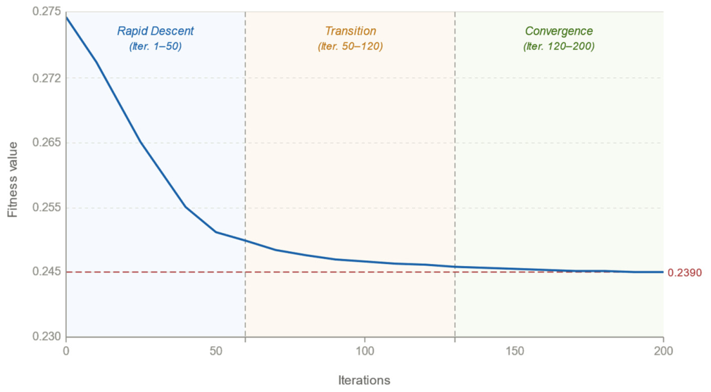
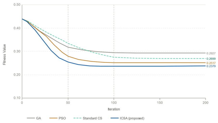
One representative scenario is randomly selected from the test set for complete iterative process visualization analysis, demonstrating the convergence characteristics of ICSA. To verify that the observed convergence behaviour is representative of the full test set rather than specific to this single scenario, Table 3 and Appendix A provide convergence statistics across all 80 test scenarios. Figure 4 presents the fitness variation curve of ICSA over 200 iterations when solving for the optimal “Grasping Pose” and optimal total motion time. As shown in the figure, the fitness variation in ICSA exhibits typical three-stage convergence characteristics. In the Rapid Descent Stage (Iterations 1–50), the fitness value rapidly decreases from 0.2742, indicating that the QUAPSO-enhanced Lévy flight update strategy preserves strong global exploration performance and enables rapid localization to high-quality solution regions. In the Transition Stage (Iterations 50–120), the fitness value continues to decrease slowly with minor fluctuations, demonstrating that the Spray Mechanism effectively prevents premature convergence by providing directional search capability during alien egg replacement. In the Convergence Stage (Iterations 120–200), the fitness value stably converges to approximately 0.2390, showcasing the robust local search capability conferred by the combined QUAPSO and Spray Mechanisms.
As shown in Table 3 and Appendix A, the three-stage convergence pattern is consistent across all 80 test scenarios. The mean final fitness value across all 80 scenarios is 0.2390 ± 0.0154, and the mean convergence iteration (defined as the number of iterations required to reach 105% of the final fitness value) is 91.6 ± 3.1 . The inter-scenario coefficient of variation in the final fitness is 6.4%, indicating well-controlled run-to-run variation. All 80 scenarios achieve final fitness values within the range [0.2106, 0.2742], and convergence iterations within [86.2, 97.1], confirming that the three-stage convergence behaviour illustrated in Figure 4 is not an artefact of scenario selection but a stable property of ICSA across diverse task configurations.
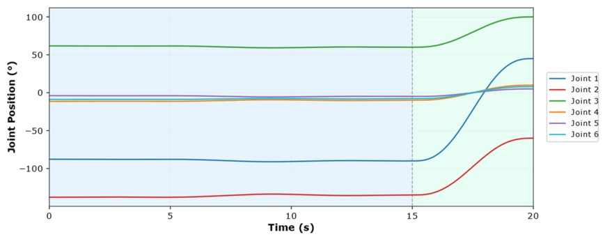
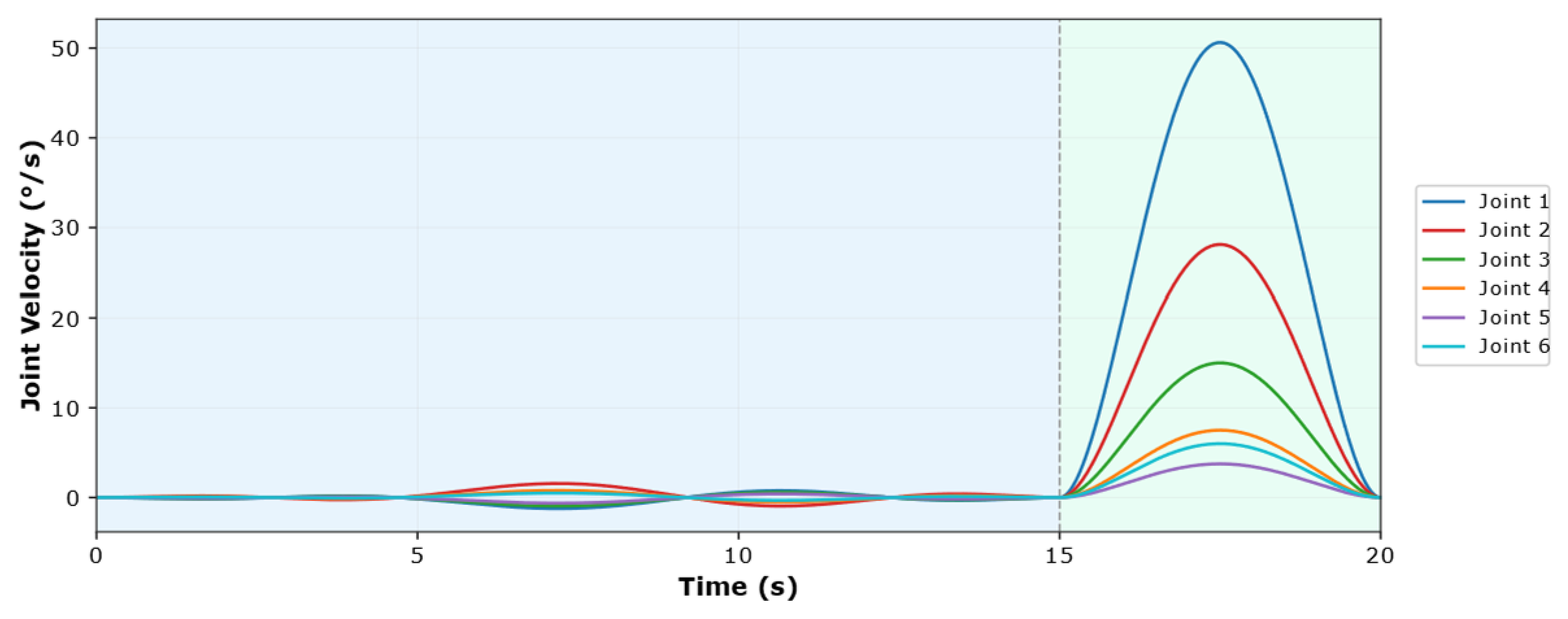
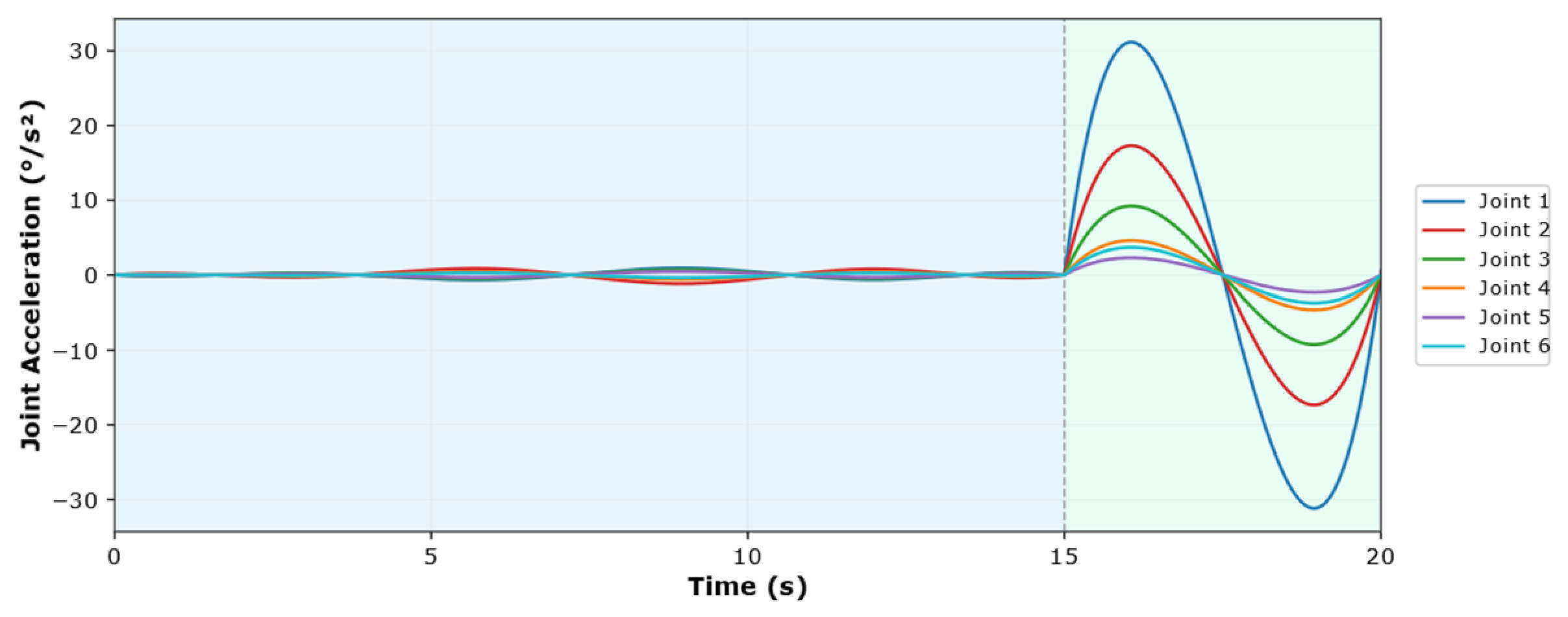
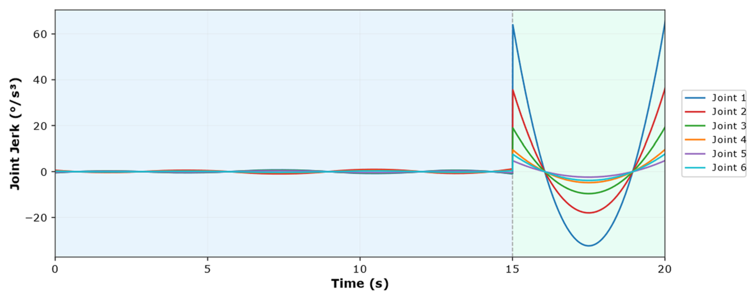
Figure 5, Figure 6, Figure 7, Figure 8 and Figure 9 respectively present the position, velocity, acceleration, jerk, and snap variation curves of the six joints throughout the complete motion trajectory. The light blue background represents the dynamic calibration trajectory phase, while the light green background represents the static execution trajectory phase. As shown in the figures, the solved optimal trajectory exhibits excellent kinematic characteristics. Figure 5 shows that all joint position curves are smooth and continuous, with no abrupt changes or step phenomena. The wrist joints (J4, J5, J6) exhibit notably smaller position variation amplitudes—within [−10°, 10°], [−5°, 5°], and [−8°, 8°] respectively—compared to the shoulder and elbow joints, effectively reducing end-effector pose fluctuations. Figure 6 shows that angular velocities of all joints converge precisely to zero at both trajectory endpoints, satisfying static-start and static-stop boundary conditions, with peak velocities strictly within V m a x m g = 180°/s. Figure 7 shows that acceleration curves likewise transition smoothly to zero at both endpoints, avoiding impact loads during start and stop. Figure 8 shows that jerk curves are continuous and bounded throughout, suppressing mechanical vibrations and joint impacts. Figure 9 shows that snap (fourth-order derivative) values remain bounded and stable, further ensuring servo drive system stability. Additionally, at the switching moment between the dynamic calibration trajectory and the static execution trajectory, both velocity and acceleration satisfy the state zeroing constraints.

6.3. Method Comparison

6.3.1. Effectiveness Validation of the ATBSC

To evaluate the effectiveness of the proposed ATBSC framework, this section presents three groups of comparative experiments using all 80 test scenarios, with each comparison method independently executed 20 times under each scenario to obtain statistically significant performance comparison results. A systematic evaluation is conducted from multiple dimensions.
(1)
Comprehensive Comparison of ATBSC with Traditional Pose-Setting Methods
To validate the advantages of ATBSC over traditional pose-setting methods, this experiment compares four methods: (a) Fixed Pose Method—directly adopting the reference configuration solved by IK as the initial solution; (b) Random Sampling Method—randomly sampling within the kinematically admissible space to generate the initial population; (c) Grid Search Method—uniform grid partitioning and sampling within the joint space; (d) ATBSC. The solving time, fitness value, convergence iteration count, constraint satisfaction rate, and trajectory quality metrics from 20 independent repeated experiments are recorded as shown in Table 4 and Figure 10.
As shown in Table 4 and Figure 10, under the simulation conditions of this study, ATBSC consistently outperforms the three baseline methods across all evaluated metrics.
In terms of solving time, ATBSC averages 1.0255 s, a 27.5% reduction over the Fixed Pose Method (1.4145 s) and a 45.8% reduction over the Grid Search Method (1.8920 s). For fitness value, ATBSC achieves 1.0312, a 20.5% improvement over the Fixed Pose Method (1.2964). Convergence requires 91.6 iterations on average, 51.0% fewer than the baseline methods in the simulation. The constraint satisfaction rate of 97.5% is markedly higher than the 72.0% of the Fixed Pose Method under these simulation conditions. In terms of trajectory quality, ATBSC reduces the total motion time to 19.82 s (an 11.7% reduction) and total energy consumption to 398.7 (a 17.9% reduction) relative to the Fixed Pose Method in the tested scenarios.
(2)
Search Space Constraint and Deviation Controllability Validation
The core advantage of ATBSC lies in reducing the effective search space through geometry-inspired bounded constraints while ensuring that the deviation between the optimized solution and the reference configuration remains within a bounded range. This experiment validates the search space reduction effectiveness and deviation controllability.
As shown in Table 5, ATBSC ( ε = 3 ° ) compresses the search space to 0.12% of the original full joint space, with a valid solution density reaching 84.7%, which is 36.8 times that of the full space (2.3%), indicating that the search space is effectively focused on high-quality solution regions; ATBSC requires only an average of 1.18 samples to obtain a feasible solution, whereas the full space requires 43.5 samples, representing an efficiency improvement of 36.9 times.
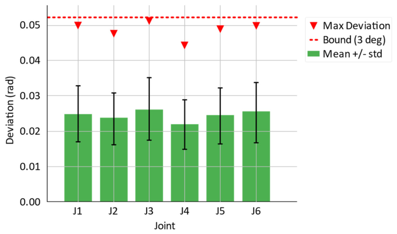
To validate the deviation controllability of ATBSC, we conducted 100 independent repeated experiments. Figure 11 presents the statistical distribution of deviations for each joint. The results demonstrate that across all 100 runs, the deviations of all six joints never exceeded the preset accuracy boundary ε m a x = 0.05236 rad (3°), and the mean deviation of each joint ranges between 0.0219~0.0261 rad, approximately 42~50% of the boundary value, indicating that the optimization process maintains a safety margin while fully utilizing the search space.
Table 6 compares the deviation performance of three methods: ATBSC reduces the average deviation from 0.0892 rad of the unconstrained method to 0.0243 rad, a reduction of 72.8%; the maximum deviation is reduced from 0.1847 rad to 0.0512 rad, a reduction of 72.3%. This demonstrates that ATBSC not only significantly reduces the mean deviation but more importantly substantially narrows the deviation distribution range, ensuring stable and controllable quality of optimized solutions.
(3)
Accuracy Boundary Parameter Analysis
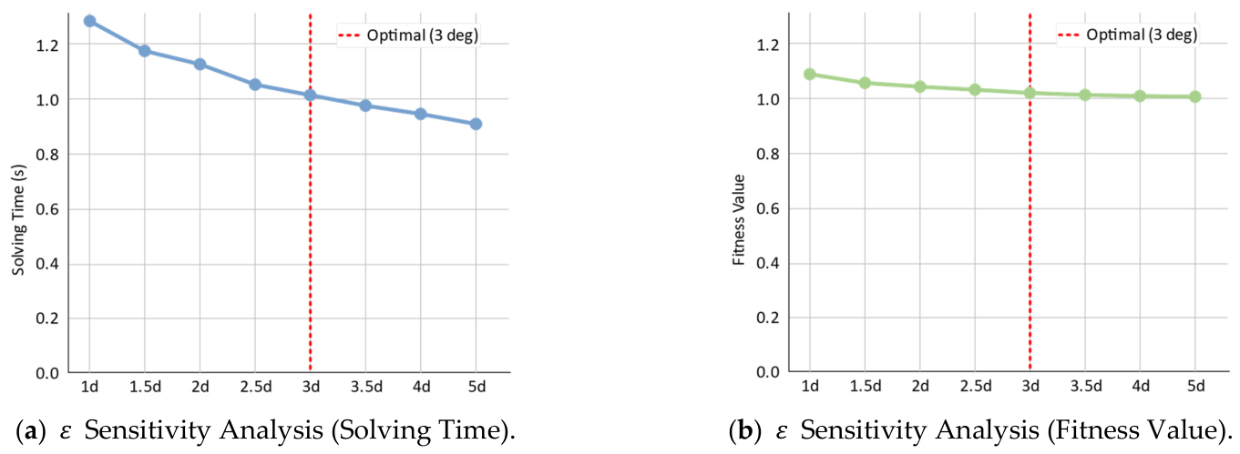
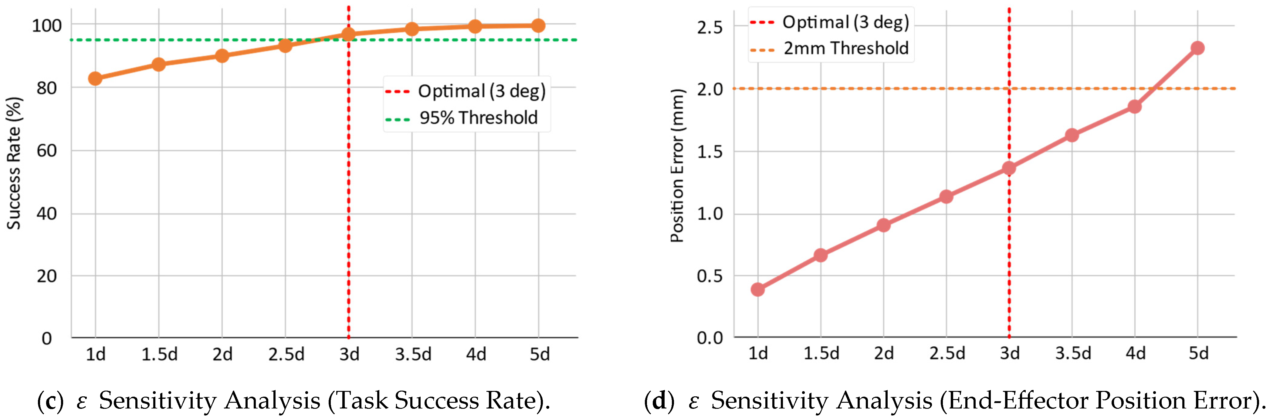
The accuracy boundary ε of the “Grasping Pose” determines the search range of the ATBSC accuracy-bounded search region. This experiment systematically tests the impact of ε values ranging from 1° to 5° on algorithm performance.
As shown in Figure 12, as ε increases, the solving time gradually decreases from 1.28 s to 0.91 s, representing an efficiency improvement of 28.9%. The fitness value decreases from 1.089 to 1.019, indicating improved solution quality. However, the end-effector position error increases from 0.42 mm to 2.31 mm. Through comprehensive analysis, ε = 3 ° represents the optimal trade-off between efficiency and precision: at this point, the success rate reaches 97%, the position error is controlled within 1.38 mm, and the orientation error is only 0.39°, satisfying the precision requirements of most industrial applications. When ε is too small (<2°), the constrained search space leads to decreased success rate; when ε is too large (>4°), although computational efficiency slightly improves, the position error exceeds the 2 mm industrial precision threshold.

6.3.2. Effectiveness Validation of the MRBCC Framework

(1)
Comparison of MRBCC with Traditional Constraint Methods
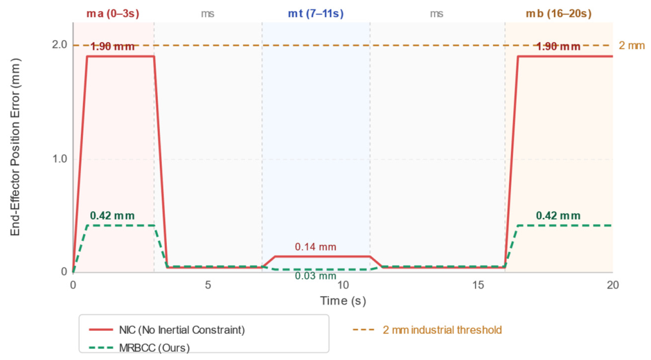
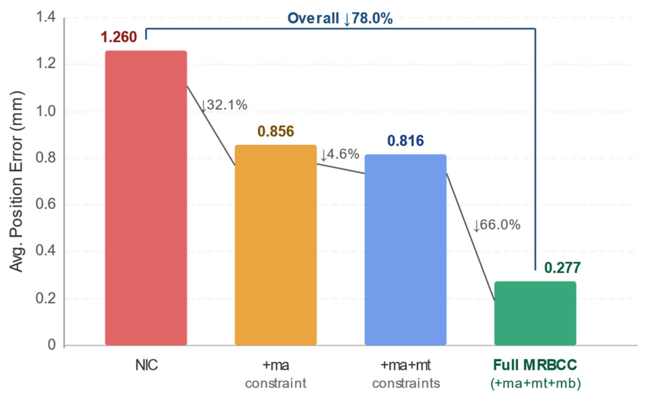
To validate the advantages of MRBCC over traditional constraint methods for the CMM, this experiment compares three methods: (a) No Inertial Constraint method (NIC)—considering only kinematic boundary constraints while ignoring inertial disturbances generated by platform motion; (b) Kinematic Constraints Only method (KCO)—adopting the kinematic constraint system from the Sequential Quadratic Programming-based method proposed by Li et al. [8], which constrains joint velocity and acceleration boundaries but does not explicitly model or compensate for inertial disturbance torques; (c) MRBCC. The experiments are conducted over the complete mobile platform motion cycle (including acceleration, constant-speed, turning, and braking phases) across all 80 test scenarios, with each scenario independently repeated 20 times, measuring the end-effector position error, orientation error, and constraint violation rate at the platform standstill moment t = T stop .
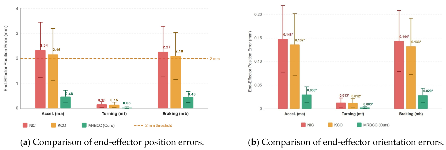
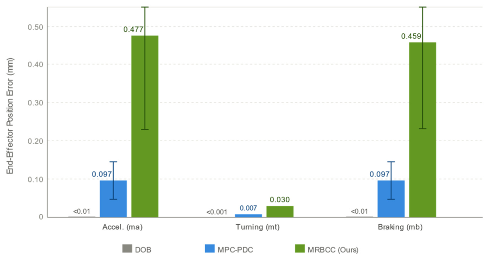
As shown in Table 7 and Figure 13, MRBCC outperforms the comparison methods across all motion phases. During the acceleration phase (ma), MRBCC reduces the end-effector position error from 2.34 mm of the NIC method to 0.48 mm, a reduction of 79.7%; compared to the KCO method (2.16 mm), the reduction is 78.0%. Notably, the position errors of NIC and KCO are nearly identical (2.34 mm vs. 2.16 mm, a difference of only 7.7%). This is physically expected: neither method applies inertial disturbance torque compensation, and their end-effector errors are governed by the same steady-state response e ss = K P 1 τ dist ( θ m , ref , a p ) . The kinematic constraints in KCO can reduce trajectory oscillations and improve smoothness (manifested as a modest 7.7% reduction), but cannot eliminate the persistent joint deviations driven by uncompensated inertial torques. During the turning phase (mt), the mean centripetal acceleration generated by platform turning is a c m t ¯ = ω m t 2 ¯ r = 0.30 2 × 0.52 = 0.047 m/s2, which is substantially lower than the mean linear acceleration a p ¯ = 0.20 m/s2 of the other phases, resulting in proportionally smaller inertial disturbances across all methods. Nevertheless, MRBCC still reduces the position error to 0.03 mm. During the braking phase (mb), MRBCC achieves a position error of 0.46 mm, representing reductions of 79.8% and 78.1% compared to the NIC and KCO methods, respectively. Regarding orientation error, the mean orientation errors of MRBCC during the acceleration, turning, and braking phases are 0.030°, 0.003°, and 0.029°, respectively, all well below the 1° industrial precision requirement. Regarding constraint violation rate, MRBCC maintains a consistent violation rate of 2.5 ± 0.6% across the three motion phases, below the 5% threshold, achieving a global constraint satisfaction rate of 97.5%. In contrast, NIC and KCO do not impose the phase-specific dynamic coupling constraints defined in Equations (15), (18) and (20), and therefore cannot provide formal guarantees of dynamic compliance.
The above results indicate that, under the simulation conditions of this study, MRBCC outperforms the comparison methods across all motion phases, indicating that the manipulator is able to reach the preset “Moving Pose” with near-zero residual velocity and acceleration at the platform standstill moment, thereby providing the deterministic initial conditions required by the full-cycle framework for the subsequent static execution trajectory. The residual errors (0.46–0.48 mm) across the three motion phases stem from first-order linearization of the coupled dynamics. These errors are strictly bounded by the ATBSC ( | θ j θ j m , r e f | ϵ j m ).
(2)
MRBCC Inertial Coupling Coefficient Robustness Analysis
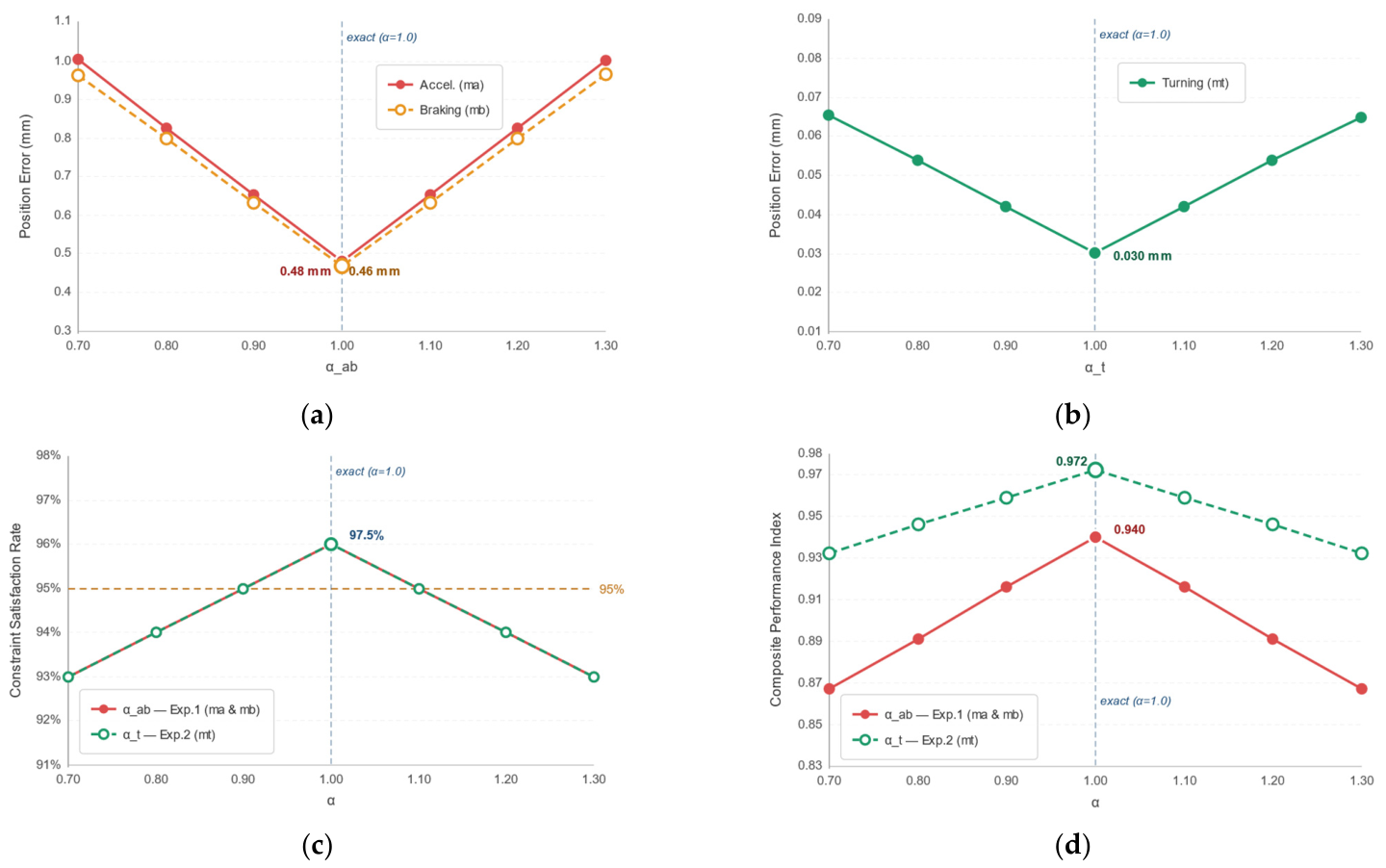
The inertial coupling coefficients k j ( ) are key parameters of the MRBCC framework. As shown in Table 2, these coefficients exhibit pronounced joint specificity: in the linear acceleration direction, from | k 5 ( a b ) | = 0.118 (J5, lowest sensitivity) to | k 2 ( a b ) | = 1.839 (J2, highest sensitivity); in the centripetal acceleration direction, from | k 4 ( t ) | = 0.032 (J4) to | k 1 ( t ) | = 1.581 (J1). In practical applications, exact values may deviate from the analytical estimates due to payload variations, unmodeled link flexibility, and linearization approximation errors. This experiment evaluates the robustness of the MRBCC framework to such parameter uncertainties by introducing a proportional perturbation factor α uniformly applied to all joints ( k j ( ) ~ = α k j ( ) , exact ), where α =   1.0 corresponds to the exact analytical values in Table 2; α <   1 represents underestimation (e.g., discrepancies between no-load and loaded conditions); α >   1 represents overestimation (conservative constraint tightening). Since the disturbance mechanisms for the linear acceleration and centripetal acceleration phases differ, the two coefficient groups are analyzed separately: Experiment 1 fixes α t = 1.0 and sweeps α a b { 0.70 , 0.80 , 0.90 , 1.00 , 1.10 , 1.20 , 1.30 } to assess the robustness of the linear acceleration direction coefficients k j ( a b ) (applicable to the acceleration and braking phases); Experiment 2 fixes α a b = 1.0 and sweeps α t over the same range to assess the robustness of the centripetal acceleration direction coefficients k j ( t ) (turning phase). Each α level is evaluated with 20 independent repetitions across all 80 test scenarios, recording end-effector position error, constraint satisfaction rate, and composite performance index.
As shown in Figure 14a, in Experiment 1, the end-effector position errors during the acceleration and braking phases exhibit a symmetric U-shaped relationship with α a b , reaching the minimum at α a b = 1.00 (exact analytical value): 0.48 mm (ma) and 0.46 mm (mb). As α a b deviates from 1.00, the errors increase symmetrically in both directions: at α a b = 0.70 (30% underestimation), errors increase to 1.00 mm (ma) and 0.96 mm (mb); at α a b = 1.30 (30% overestimation), errors similarly increase to 1.00 mm and 0.97 mm. This symmetry confirms that both underestimation and overestimation of the coupling coefficients lead to comparable performance degradation—underestimation results in insufficient disturbance compensation, while overestimation results in over-tightened constraints on the calibration trajectory, reducing its flexibility.
As shown in Figure 14b, in Experiment 2, the turning phase error likewise exhibits a symmetric pattern centered at α t = 1.00 (0.030 mm), increasing to 0.066 mm and 0.065 mm at α t = 0.70 and α t = 1.30 , respectively. The absolute error values are smaller than those in the linear acceleration phases, consistent with the lower centripetal acceleration magnitudes in Table 1, indicating that the turning phase coefficients k j ( t ) have less stringent precision requirements compared to the linear acceleration phase coefficients.
As shown in Figure 14c, the constraint satisfaction rate exhibits a symmetric inverted U-shaped relationship with α , with both experimental groups peaking at α =   1.00 (97.5%) and monotonically decreasing as α deviates from 1.00. For both the α a b and α t groups, the satisfaction rate remains above 96.0% within α [ 0.90 , 1.10 ] (exact value ± 10%); and above 94.5% within α [ 0.80 , 1.20 ] (±20%). This demonstrates that even under moderate uncertainty in coupling coefficient estimates, the MRBCC framework maintains acceptable constraint compliance.
As shown in Figure 14d, the composite performance index (simultaneously accounting for position error and constraint satisfaction rate) confirms that both experimental groups reach the optimum at α =   1.00 (0.940 for the α a b group; 0.972 for the α t group). The α t curve outperforms the α a b curve at all α values, reflecting the lower absolute contribution of centripetal disturbances to overall performance during platform operation. The flat optimal region near α =   1.00 —with the α a b composite index remaining above 0.91 within α [ 0.90 , 1.10 ] —further validates the practical robustness of the analytical coefficient derivation in Table 2: setting α within a physically reasonable range near the analytical values is sufficient to ensure effective operation of the MRBCC framework.
(3)
Temporal Error Analysis and Ablation Experiment
To further validate the suppression effectiveness of MRBCC on inertial disturbances throughout the complete motion cycle of the mobile platform, this experiment sets up a fixed test scenario with a total motion time of 20 s, comprising 5 sequentially executed phases: acceleration (ma, 0–3 s, a p = 0.20 m/s2), constant-speed (ms, 3–7 s), turning (mt, 7–11 s, ω m t = 0.30 rad/s), constant-speed (ms, 11–16 s), and braking (mb, 16–20 s, a p = 0.20 m/s2). The end-effector position error temporal curve throughout the entire Moving Phase is recorded, and the contribution of each constraint component is analyzed through ablation experiments.
As shown in Figure 15, the NIC method produces peak position errors of 1.90 mm during the acceleration (ma) and braking (mb) phases, approaching but still within the 2 mm industrial precision threshold. The peak during the turning phase (mt) is only 0.14 mm, consistent with the lower centripetal acceleration ( a c m t ¯ = 0.047 m/s2) at the operating speed of the mobile platform. In contrast, the MRBCC method keeps the end-effector error within 0.42 mm throughout the entire Moving Phase (0.42 mm during the ma and mb phases; 0.03 mm during the mt phase), providing substantially greater precision margins below the industrial threshold.
As shown in the ablation experiment results (Figure 16), starting from the NIC baseline (mean error across dynamic phases: 1.26 mm), adding the acceleration phase constraint (+ma) reduces the error to 0.856 mm, a reduction of 32.1%; further adding the turning phase constraint (+ma+mt) marginally reduces the error to 0.816 mm (a further reduction of 4.6%), because the centripetal disturbance during the turning phase is relatively small at the operating speed of the mobile platform; adding the braking phase constraint to complete the full MRBCC framework yields the largest reduction, bringing the error down to 0.277 mm (a further reduction of 66.0%), because the braking phase has the longest duration (4 s) in this scenario and thus the highest cumulative disturbance contribution. The full MRBCC framework achieves an overall reduction of 78.0% relative to NIC.
The ablation results confirm that all three constraint components make positive contributions, with their relative magnitudes reflecting the disturbance intensity and phase duration of each motion phase: the braking phase constraint contributes the most due to its long duration; the acceleration phase constraint contributes significantly due to comparable linear acceleration magnitudes; and the turning phase constraint contributes the least due to the lower centripetal acceleration at the operating speed of the mobile platform. This validates the necessity of the phase-specific constraint design in the MRBCC framework.
(4)
Comparison with Mobile Manipulator-Specific Disturbance Rejection Methods
This section compares MRBCC with two representative mobile manipulator-specific disturbance rejection control-layer baseline methods: (a) Disturbance Observer-Based Control (DOB), implemented following the coupled dynamics modeling framework of Zhou et al. [3], in which joint-level disturbance observers estimate inertial disturbance torques via low-pass filtering (cutoff frequency 10 Hz) and apply real-time compensation; (b) Model Predictive Disturbance Compensation (MPC-PDC), implemented following the framework of Tao et al. [22], which utilizes DT-predicted platform motion time series and solves a quadratic programming tracking problem at each 5 ms control cycle (prediction horizon: 10 steps, 6 joints). The experiments are conducted across all 80 test scenarios, with 20 independent repetitions per scenario. It should be noted that MRBCC operates at the planning layer: the analytically derived inertial coupling constraints from Table 2 are embedded into the dynamic calibration trajectory prior to execution, causing the manipulator to converge to θ m , ref at t = T stop by design, with zero online computation during execution. DOB and MPC-PDC operate at the control layer: they estimate or predict disturbance torques at each control cycle and apply compensating joint commands. These two paradigms address the same disturbance problem at different architectural layers and are complementary rather than competing; accordingly, the following comparison is organized around the dimensions where genuine differences exist.
As shown in Figure 17 and Table 8, under planned platform disturbances, DOB achieves near-zero position errors across all three motion phases (ma: 0.002 mm; mt: <0.001 mm; mb: 0.002 mm), and MPC-PDC likewise achieves very low errors (ma/mb: 0.097 mm; mt: 0.007 mm). MRBCC retains larger residuals (ma: 0.477 mm; mb: 0.459 mm; mt: 0.030 mm); for the dominant linear acceleration phases, DOB and MPC-PDC reduce errors by 99.6% and 79.7% relative to MRBCC, respectively. This ranking is physically expected: DOB and MPC-PDC directly cancel disturbance torques at the joint layer, achieving near-perfect compensation for the predictable, low-frequency platform accelerations in Table 1. MRBCC retains approximately 22% of the nominal disturbance response residual, bounded by the ATBSC ε j m ; this is a first-order linearization error of the coupled dynamics at θ m , ref , rather than uncompensated torque. However, end-effector position error is neither the sole metric nor the most operationally meaningful metric for evaluating disturbance handling strategies within the full-cycle parallel planning framework.
Table 8 summarizes the multi-dimensional comparison. Regarding execution-time computational overhead: MRBCC incurs zero additional computation during execution; DOB requires approximately 0.8 ms per control cycle; MPC-PDC requires approximately 7.5 ms per control cycle, equivalent to 150% of the 5 ms control cycle. Regarding constraint satisfaction guarantees: MRBCC guarantees a 97.5% satisfaction rate of the MRBCC phase-specific trajectory constraints through planning-layer design; DOB and MPC-PDC, as reactive control-layer methods, do not provide formal guarantees of such constraint-level trajectory compliance. Regarding planning-layer integration: MRBCC is natively integrated with the full-cycle parallel planning architecture without requiring modifications to joint servo controllers; DOB and MPC-PDC require dedicated sensing hardware, real-time communication interfaces, and controller reconfiguration, which are orthogonal to the planning layer.
In summary, the three methods reflect different architectural trade-offs in the mobile manipulator control stack. Control-layer methods (DOB, MPC-PDC) achieve superior end-effector precision under known platform disturbances, at the cost of execution-time computational overhead and lack of planning-layer constraint guarantees. MRBCC, at the cost of larger steady-state residuals (0.46–0.48 mm for the linear acceleration-dominated phases), prioritizes zero execution-time overhead, deterministic initial conditions, and planning-layer constraint satisfaction, although these residuals remain below the 2 mm industrial precision threshold. These trade-offs are complementary; a hybrid architecture combining MRBCC’s planning-layer guarantees with a lightweight DOB (for residual correction) is a natural future extension, which we identify as a direction for further research in Section 7.

6.3.3. Integrated Effectiveness Validation of the Full-Cycle Spatiotemporally Coupled Method

To evaluate the practical contribution of the full-cycle spatiotemporally coupled framework in eliminating decision latency and enhancing system throughput, this section compares the full-cycle operation duration of the serial and parallel paradigms based on all 80 test scenarios. The two execution paradigms are defined as follows:
(a)
Serial Paradigm: The planning of the static execution trajectory is triggered only after the mobile platform has come to a complete standstill at t = 15   s , resulting in a mandatory decision latency of Δ t d e l a y = t s o l v e .
(b)
Full-Cycle Spatiotemporally Coupled Parallel Paradigm (Proposed): The static execution trajectory is optimized concurrently during the platform movement phase. As long as t s o l v e T m o v e is satisfied, the trajectory can be triggered immediately at the moment of platform standstill, effectively reducing Δ t d e l a y to zero.
The full-cycle duration is measured from the moment the platform initiates movement until the completion of the grasping task, with results summarized in Figure 18 and Table 9 and Table 10.
As illustrated in Table 9 and Figure 18a, the serial paradigm must wait for the completion of trajectory planning after braking, with a mandatory decision latency of 1.841   ± 0.136   s . In contrast, the parallel paradigm effectively eliminates this latency in all 80 tested scenarios (where t s o l v e T m o v e is satisfied throughout), enabling the system to trigger the pre-planned static execution trajectory with zero delay at the moment the platform stops at t = 15 s.
The proposed method reduces the mean full-cycle duration from 21.688   ± 0.163   s to 19.827   ± 0.114   s , achieving an overall operational efficiency improvement of 8.58%. This reduction (1.861 s) corresponds directly to the eliminated decision latency, while the duration of the static execution phase remains virtually unchanged (4.848 s vs. 4.827 s, a difference of only 0.4%). This suggests that, under the tested simulation conditions, the parallel planning mechanism does not compromise trajectory quality.
The box plot in Figure 18b further demonstrates that the parallel paradigm exhibits significantly lower variance (standard deviation of 0.114 s vs. 0.163 s, a 30.1% reduction). This indicates more consistent task completion times across diverse operating conditions. Furthermore, the Interquartile Range (Q3−Q1) of the parallel paradigm (0.11 s) is much smaller than that of the serial paradigm (0.21 s). Within the obstacle-free simulation scope of this study, this enhanced predictability suggests potential benefits for multi-robot synchronization and coordination in flexible manufacturing environments; whether this advantage is preserved in environments with dynamic obstacles or cluttered workspaces remains a direction for future investigation.
This improvement holds particular practical significance in high-tempo flexible manufacturing scenarios involving repetitive task cycles, within the obstacle-free simulation scope of this study. As an illustrative estimate under the simulation conditions, for a production facility executing 500 grasping operations per shift in an obstacle-free environment, the proposed method would recover approximately 500 × 1.841 = 920 s of effective production time per shift compared to the serial paradigm. It should be noted that this estimate is derived from the obstacle-free simulation results and assumes ideal DT prediction conditions; actual throughput gains in real deployments—where dynamic obstacles, sensor noise, and model uncertainty are present—may differ and would require independent validation. Within the validated scope, when the optimization algorithm’s logic is complex and decision latency is non-negligible, the proposed full-cycle spatiotemporally coupled method indicates the potential to significantly suppress non-productive pauses during task execution in obstacle-free flexible manufacturing workflows.


6.3.4. Parameter Transfer Validation: Sensitivity to Platform Dynamic Parameters

This section investigates the sensitivity of the MRBCC framework to platform dynamic parameter variation by transferring the experimentally validated physical parameters of Zhou et al. [3]—including mobile platform mass/moments of inertia and robotic arm link masses/inertia tensors—into the simulation environment of this study. It should be noted that since task-level parameters (initial and target end-effector positions, motion phase durations) were not reported in [3], they continue to be generated via the randomisation procedure described in Section 6.1. Accordingly, this section does not constitute a cross-study benchmark in the strict sense; rather, it evaluates whether the relative performance advantage of MRBCC is maintained when the platform dynamic parameters are replaced with those of an independently validated physical system operating at a higher characteristic acceleration ( a p = 0.35 m/s2, approximately 1.75 times the mean value used in the main test set). The characteristic linear acceleration ( a p = 0.35 m/s2) and turning angular velocity ( ω m t = 0.25 rad/s), which corresponds to a centripetal acceleration of a c = 0.033 m/s2, are drawn from the experimental motion data recorded in [3], reflecting the typical operational range of industrial AGV platforms.
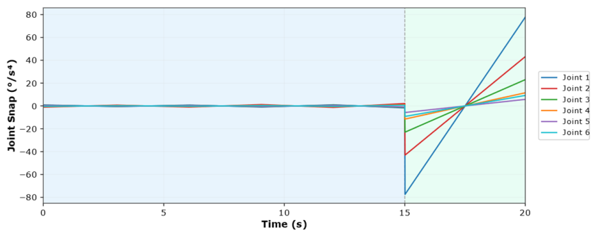
As shown in Table 11, when the platform dynamic parameters are replaced with those from [3], the error reduction of MRBCC relative to NIC remains at 78.0%, identical to that observed in the original MiR 200 test scenarios. This consistency demonstrates that the relative performance advantage of MRBCC over inertia-agnostic baselines is robust to substantial variation in platform dynamic parameters—specifically, to an increase of approximately 1.75× in characteristic linear acceleration. The constraint satisfaction rate under [3] parameters is 96.8%, slightly lower than the 97.5% in the main test set; this aligns with the physical expectation that higher platform acceleration leads to tighter inertial coupling constraints. Notably, the absolute position error of MRBCC (0.732 mm) remains well below the 2 mm industrial precision threshold even under the stronger disturbances produced by the [3] parameters, confirming that the MRBCC framework maintains its practical engineering utility across the range of platform dynamic configurations tested.
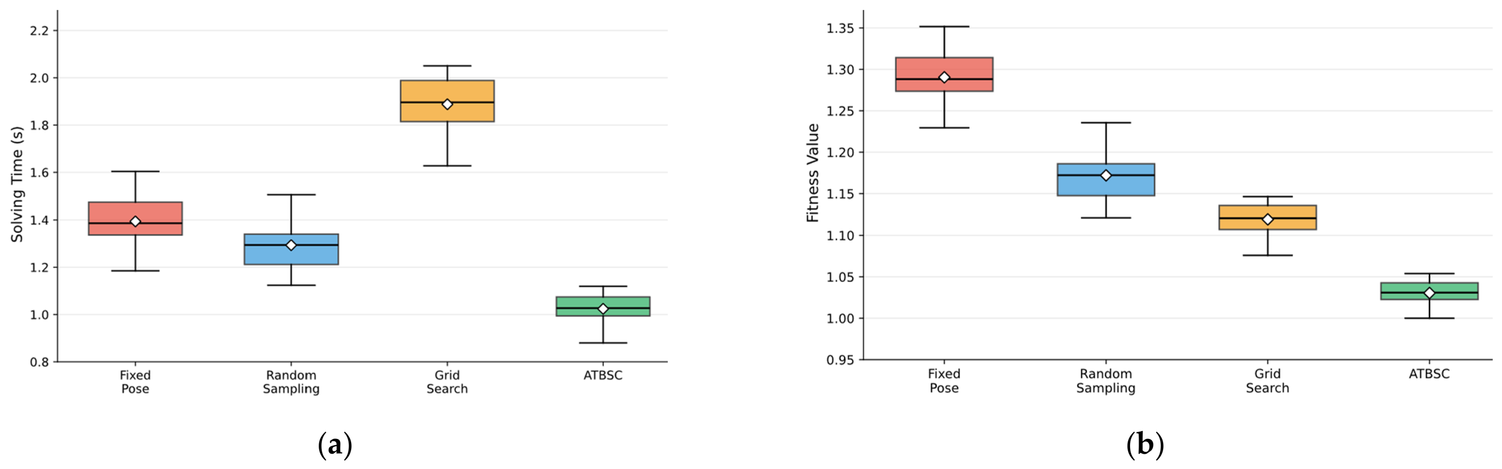
6.3.5. Algorithm Performance Comparison

To validate the performance advantages of ICSA, this section compares it with the standard Genetic Algorithm (GA), standard Particle Swarm Optimization (PSO), and standard CS algorithm through comparative experiments. Twenty representative scenarios are randomly selected from the test set, and all algorithms adopt identical population sizes (N = 100) and maximum iteration counts (M = 200) as specified in Table 12. It should be noted that ICSA is proposed as a population-based metaheuristic and is evaluated against algorithms of the same class that share the same problem representation and constraint interface (direct penalty-function encoding of MRBCC phase-switching constraints). Comparison against gradient-based specialised planners (e.g., TrajOpt, STOMP, CHOMP) is beyond the scope of this evaluation, as those methods require fundamentally different problem formulations that cannot directly accommodate the non-smooth phase-switching constraints introduced by MRBCC without substantial algorithmic reformulation.
As shown in Figure 19, the four algorithms exhibit distinct convergence behaviors. In the early stage (iterations 1–50), ICSA achieves the fastest descent rate among the CS-family algorithms, with the fitness value decreasing rapidly from its initial value, driven by the QUAPSO mechanism’s enhanced global exploration capability. Standard CS decreases more slowly over the same interval. In the mid-stage (iterations 50–120), the descent rates of GA and standard CS noticeably slow down, whereas ICSA maintains a stable convergence trend attributable to the Spray Mechanism’s directional alien egg replacement strategy. In the final convergence stage (iterations 120–200), ICSA stably converges to a mean fitness value of 0.2379, outperforming standard CS (0.2699), GA (0.2927), and PSO (0.2517). The detailed statistical results are presented in Table 13. Compared to the standard CS algorithm, ICSA achieves a fitness improvement of 11.9% and a convergence speed improvement of 13.1%, where convergence speed is defined as the reduction in iterations required to reach 105% of the final fitness value (CS: 107 iterations; ICSA: 93 iterations). Importantly, ICSA achieves the lowest standard deviation (0.0258) among all four algorithms, indicating superior solution stability and robustness across diverse scenarios—a property of particular importance for industrial applications where consistent performance is required across varying task configurations. These results validate that the integration of the QUAPSO mechanism and Spray Mechanism effectively enhances both convergence efficiency and solution consistency of the standard CS baseline.

6.3.6. Weight Sensitivity Analysis

To evaluate the robustness of the adopted objective weight allocation ( ω T = 0.5 , ω E = 0.3 , ω S = 0.2 ), this section presents a systematic sensitivity experiment. ω T is varied across eight levels from 0.1 to 0.8; the remaining weight budget is allocated to ω E and ω S in a fixed 3:2 ratio consistent with their baseline proportions. All 80 test scenarios are evaluated with 20 independent runs per scenario. Four metrics are recorded: total motion time, energy consumption, normalised smoothness index (1.0 = baseline), and overall fitness value (jointly with constraint satisfaction rate CSR). The results are summarised in Table 14 and Figure 20.
As shown in Figure 20a, total motion time decreases monotonically from 21.08 s ( ω T   =   0.1 ) to 18.84 s ( ω T = 0.8 ) as time is increasingly prioritised. Figure 20b shows that energy consumption increases correspondingly from 314.2 to 461.2 as ω E decreases, reflecting the expected time-energy trade-off. Figure 20c demonstrates that trajectory smoothness degrades (normalised index increases from 0.517 to 1.387) as ω S decreases. Figure 20d shows that the fitness value achieves its minimum of 0.2390 at the baseline ( ω T = 0.5 ), increasing by at most 0.0078 across the full weight range tested—a variation of only 3.3% relative to the baseline. The CSR remains consistently above 95.8% for all tested configurations, confirming that the MRBCC structure is insensitive to objective weight variation. These results confirm that the framework performance is robust to moderate weight perturbations.

7. Discussion

This paper addresses the dynamic decoupling problem of multi-rigid-body nonlinear inertial disturbances in the CMM within flexible manufacturing systems, proposing a full-cycle spatiotemporally coupled optimal trajectory planning method. This method bifurcates the manipulator motion trajectory into two stages: “dynamic calibration” and “static execution”, eliminating decision latency through temporal parallel pre-planning and suppressing inertial disturbances through spatial proactive compensation. Within this framework, this paper further proposes two key technologies: (1) the ATBSC framework, which, in the simulation-based evaluation, compresses the search space to 0.12% of the original full joint space, increases the valid solution density from 2.3% to 84.7%, and reduces the average deviation by 72.8%; (2) the MRBCC system, which explicitly models the inertial disturbance transmission process during each motion phase and, under the tested simulation conditions, reduces end-effector position errors by 79.7%, 81.0%, and 79.8% during the acceleration, turning, and braking phases, respectively, with a constraint satisfaction rate of 97.5%. Meanwhile, the ICSA integrating the QUAPSO mechanism and Spray Mechanism reduces the fitness value by approximately 11.9% compared to the standard CS algorithm and improves the convergence speed by approximately 13.1% in the tested scenarios.
This study also has several limitations. First, the validation results are obtained under two idealising assumptions. (a) The global path planning scheme of the CMM platform—including motion phase durations and characteristic accelerations—is assumed to be known a priori before platform initiation, which is equivalent to a DT output with zero prediction error under known-path conditions. In practical deployment, path deviations caused by localisation uncertainty, dynamic obstacles, or AMR control jitter would introduce discrepancies between the planned and executed motion phases. (b) The paper assumes zero discrepancy between DT predictions and actual platform motion data. Under this assumption, the MRBCC constraint system receives exact characteristic accelerations as inputs, and the reported position error reductions represent the performance achievable under ideal DT conditions. In physical deployment, DT prediction errors—arising from model uncertainty, sensor noise, and unmodeled platform dynamics—would propagate into the MRBCC constraint bounds and may degrade trajectory quality relative to the simulation-based results. Quantifying the sensitivity of the MRBCC framework to DT prediction error, and designing robust trajectory planning strategies that remain effective under bounded path uncertainty, are identified as important directions for future work. Second, the restriction to an obstacle-free environment is a key limitation. In the future, we plan to extend the MRBCC framework to dynamic obstacle environments and to investigate the collaborative optimization mechanism between inertial disturbance compensation and obstacle avoidance. Third, due to the difficulty in obtaining a physical CMM platform during the study, the experimental validation is based entirely on simulation. It is important to note that the parameter transfer validation presented in Section 6.3.4, while it introduces the experimentally validated platform dynamic parameters of Zhou et al. [3] into the simulation environment, remains a simulation-based sensitivity analysis: it evaluates the robustness of the relative performance advantage of MRBCC to variation in platform dynamic parameters, but does not constitute—nor is it intended to replace—physical hardware validation. The gap between a simulation test conducted with physically validated parameters and an experiment executed on a real CMM platform remains substantial, as the latter involves sensor noise, actuator nonlinearities, model uncertainty, unmodeled structural flexibility, and real-time communication constraints that cannot be fully captured in simulation. Deploying the proposed full-cycle spatiotemporally coupled framework on a real CMM platform to verify its engineering practicality under real conditions—including sensor noise, model uncertainty, actuator saturation, and unmodeled external disturbances—is therefore identified as the primary near-term priority for future experimental work. We also plan to extend our research in the following directions. First, investigating whether reinforcement learning-based policies can be trained to satisfy the phase-specific inertial coupling constraints of the MRBCC system—while providing formal constraint satisfaction guarantees comparable to those of the planning-layer approach—represents a promising avenue for future work. Second, the proposed framework is scalable regarding the number of degrees of freedom of the manipulator, and extending it to multi-robot collaborative systems in a shared workspace is a promising but significantly more complex direction for our future research. Third, Section 6.3.4 of the present manuscript evaluates the sensitivity of MRBCC to platform dynamic parameter variation within the simulation environment by substituting the experimentally validated parameters of Zhou et al. [3]; a genuine cross-study validation using the actual task-level parameters from [3] on the same physical platform is identified as a near-term priority for future experimental work, and represents a distinct and higher level of external validation than the parameter transfer analysis already completed. Fourth, and most critically, the entire experimental validation of this study—including both the main 80-scenario test set and the parameter transfer validation in Section 6.3.4—is conducted in simulation. Real hardware validation on a physical CMM platform, which would expose the framework to sensor noise, actuator nonlinearities, model uncertainty, unmodeled structural flexibility, and real-time communication constraints absent from the simulation, is the primary hardware validation goal for our future work and will be pursued as a matter of priority.

Author Contributions

Conceptualization, writing—review and editing, H.X., Z.S. and H.T.; Methodology, data curation, Z.S. and L.W.; Funding acquisition, H.X.; Supervision, H.T. and L.W. All authors have read and agreed to the published version of the manuscript.

Funding

The work was supported by Basic Science (Natural Science) Research Project of Higher Education Institutions of Jiangsu Province (23KJB62006), the Humanities and Social Sciences Program of the Ministry of Education (23YJCZH201), Jiangsu Social Science Foundation (23GLLC015), National Natural Science Foundation of China (72401128), Natural Science Foundation of Jiangsu Province (BK20240537), National Social Science Fund of China (21CJY055) and the Qing Lan Project of Jiangsu Provincial Higher Education Institutions (54905013).

Data Availability Statement

Data will be made available on request.

Conflicts of Interest

The authors declare no conflicts of interest.

Appendix A

Table A1 reports the ICSA convergence statistics for all 80 test scenarios in the complete test set (Section 6.1), constructed following the randomisation procedure described therein. Each scenario is independently repeated 20 times with identical ICSA parameter settings (Table 12). Final fitness: mean and standard deviation of the best fitness value at iteration 200 across 20 runs. Conv. Iter.: mean and standard deviation of the number of iterations required to reach 105% of the final fitness value across 20 runs.
Table A1. ICSA Convergence Statistics for All 80 Test Scenarios (20 independent runs each).
ScenarioFinal Fitness (Mean ± Std)Conv. Iter. (Mean ± Std)
S010.2422 ± 0.015992.0 ± 2.7
S020.2462 ± 0.020197.1 ± 2.5
S030.2439 ± 0.021391.7 ± 2.9
S040.2430 ± 0.011889.7 ± 2.6
S050.2387 ± 0.020289.3 ± 2.2
S060.2742 ± 0.017892.5 ± 2.6
S070.2395 ± 0.016295.1 ± 4.0
S080.2333 ± 0.016993.8 ± 2.2
S090.2216 ± 0.018386.2 ± 2.5
S100.2106 ± 0.019892.5 ± 3.2
S110.2388 ± 0.017588.3 ± 2.6
S120.2307 ± 0.019792.2 ± 3.4
S130.2497 ± 0.015095.0 ± 3.9
S140.2315 ± 0.018989.0 ± 2.3
S150.2614 ± 0.023990.7 ± 1.7
S160.2741 ± 0.016492.3 ± 2.8
S170.2382 ± 0.017486.7 ± 2.5
S180.2212 ± 0.016592.8 ± 2.0
S190.2569 ± 0.016891.5 ± 2.8
S200.2435 ± 0.021793.7 ± 2.8
S210.2419 ± 0.019490.1 ± 2.9
S220.2429 ± 0.020795.0 ± 2.2
S230.2107 ± 0.017891.3 ± 3.4
S240.2444 ± 0.014990.7 ± 2.9
S250.2411 ± 0.028492.0 ± 2.9
S260.2474 ± 0.019391.7 ± 2.5
S270.2208 ± 0.022290.0 ± 3.4
S280.2513 ± 0.021591.2 ± 3.4
S290.2519 ± 0.016292.8 ± 2.8
S300.2450 ± 0.019992.0 ± 3.4
S310.2266 ± 0.015295.6 ± 3.3
S320.2537 ± 0.018393.0 ± 2.8
S330.2402 ± 0.014695.9 ± 2.6
S340.2280 ± 0.020091.1 ± 2.3
S350.2530 ± 0.018292.2 ± 3.4
S360.2717 ± 0.013895.9 ± 2.6
S370.2230 ± 0.013492.2 ± 2.4
S380.2350 ± 0.018689.5 ± 3.1
S390.2293 ± 0.020592.2 ± 3.3
S400.2295 ± 0.018292.6 ± 2.4
S410.2112 ± 0.012297.9 ± 2.5
S420.2455 ± 0.019190.0 ± 2.4
S430.2475 ± 0.013892.0 ± 2.3
S440.2106 ± 0.017890.3 ± 2.8
S450.2212 ± 0.018994.2 ± 2.6
S460.2187 ± 0.018687.3 ± 2.7
S470.2459 ± 0.017786.6 ± 2.7
S480.2350 ± 0.019890.5 ± 2.7
S490.2372 ± 0.022488.9 ± 3.2
S500.2250 ± 0.018892.5 ± 3.4
S510.2408 ± 0.017186.3 ± 3.1
S520.2250 ± 0.013294.2 ± 2.8
S530.2650 ± 0.017288.0 ± 2.5
S540.2353 ± 0.018891.8 ± 3.0
S550.2270 ± 0.017591.9 ± 2.0
S560.2535 ± 0.024590.7 ± 3.8
S570.2387 ± 0.019385.2 ± 1.9
S580.2164 ± 0.019890.3 ± 2.4
S590.2154 ± 0.019387.0 ± 2.4
S600.2842 ± 0.013790.7 ± 2.9
S610.2381 ± 0.018792.0 ± 2.4
S620.2137 ± 0.021397.8 ± 3.2
S630.2400 ± 0.020689.8 ± 2.3
S640.2600 ± 0.018895.0 ± 2.9
S650.2328 ± 0.016499.8 ± 1.9
S660.2338 ± 0.023389.9 ± 2.9
S670.2483 ± 0.018697.0 ± 2.9
S680.2539 ± 0.019687.4 ± 2.4
S690.2442 ± 0.015994.2 ± 3.2
S700.2592 ± 0.019789.6 ± 2.4
S710.2411 ± 0.021897.2 ± 2.4
S720.2409 ± 0.018587.0 ± 3.5
S730.2328 ± 0.013892.0 ± 2.3
S740.2226 ± 0.017595.5 ± 2.3
S750.2542 ± 0.015586.7 ± 2.5
S760.2364 ± 0.016089.9 ± 2.7
S770.2263 ± 0.019288.8 ± 2.8
S780.2548 ± 0.016491.0 ± 2.3
S790.2282 ± 0.018496.6 ± 2.8
S800.2331 ± 0.020188.8 ± 2.4
Overall Mean ± Std0.2390 ± 0.015491.6 ± 3.1

References

  1. Ghodsian, N.; Benfriha, K.; Olabi, A.; Gopinath, V.; Arnou, A. Mobile manipulators in industry 4.0: A review of developments for industrial applications. Sensors 2023, 23, 8026. [Google Scholar] [CrossRef] [PubMed]
  2. Feng, Y.; Tian, X.; Li, T.; Jiang, Y. Measurement of mobile manipulator chassis pose change caused by suspension deformation and end-effector accuracy improvement based on multi-sensor fusion. Robot. Auton. Syst. 2023, 170, 104553. [Google Scholar] [CrossRef]
  3. Zhou, Z.; Yang, X.; Wang, H.; Zhang, X. Coupled dynamic modeling and experimental validation of a collaborative industrial mobile manipulator with human-robot interaction. Mech. Mach. Theory 2022, 176, 105025. [Google Scholar] [CrossRef]
  4. Sandakalum, T.; Ang, M.H., Jr. Motion planning for mobile manipulators—A systematic review. Machines 2022, 10, 97. [Google Scholar] [CrossRef]
  5. Xie, D.J.; Zeng, L.D.; Xu, Z.; Guo, S.; Cui, G.H.; Song, T. Base position planning of mobile manipulators for assembly tasks in construction environments. Adv. Manuf. 2023, 11, 93–110. [Google Scholar] [CrossRef]
  6. Flori, A.; Oulhadj, H.; Siarry, P. QUAntum Particle Swarm Optimization: An auto-adaptive PSO for local and global optimization. Comput. Optim. Appl. 2022, 82, 525–559. [Google Scholar] [CrossRef]
  7. Fang, M.; Xu, Z.; Gai, Y.; Ye, D.; Liu, T.; Tan, P.; Tan, K. Path planning for mobile manipulator based on energy consumption and grasping accuracy constraints. AIP Adv. 2025, 15, 125335. [Google Scholar] [CrossRef]
  8. Li, Y.; Wang, Z.; Yang, H.; Zhang, H.; Wei, Y. Energy-Optimal Planning of Robot Trajectory Based on Dynamics. Arab. J. Sci. Eng. 2023, 48, 3523–3536. [Google Scholar] [CrossRef]
  9. Xia, X.; Li, T.; Sang, S.; Cheng, Y.; Ma, H.; Zhang, Q.; Yang, K. Path planning for obstacle avoidance of robot arm based on improved potential field method. Sensors 2023, 23, 3754. [Google Scholar] [CrossRef] [PubMed]
  10. Zhang, J.; Yang, F.; Nie, G.; Zhang, J. Optimal Trajectory Planning for Minimizing Base Disturbance of a Redundant Space Robot with IQPSO. J. Electr. Comput. Eng. 2022, 2022, 3398810. [Google Scholar] [CrossRef]
  11. Xiao, P.; Zhou, J.; Zhou, C.; Si, Y.; Zhou, D. Non-Holonomic Path Planning for Space Robots Based on Jerk Constraints. Int. J. Astronaut. Aeronaut. Eng. 2023, 8, 65. [Google Scholar]
  12. Chen, W.; Wang, H.; Liu, Z.; Jiang, K. Time-energy-jerk optimal trajectory planning for high-speed parallel manipulator based on quantum-behaved particle swarm optimization algorithm and quintic B-spline. Eng. Appl. Artif. Intell. 2023, 126, 107223. [Google Scholar] [CrossRef]
  13. Lopez-Franco, C.; Diaz, D.; Hernandez-Barragan, J.; Arana-Daniel, N.; Lopez-Franco, M. A metaheuristic optimization approach for trajectory tracking of robot manipulators. Mathematics 2022, 10, 1051. [Google Scholar] [CrossRef]
  14. Hussein, R.M.; Hadi, A.S.; Hasan, S.F.; Al-Haddad, L.A.; Harrabi, R.; Flah, A.; Sahib, I.A.A. Hybrid integral sliding mode and fuzzy logic control for omnidirectional robots: Modified elephant herding optimization for trajectory tracking. Sci. Rep. 2025, 15, 35666. [Google Scholar] [CrossRef] [PubMed]
  15. Yang, X.-S.; Deb, S. Cuckoo search via Lévy flights. In Proceedings of the 2009 World Congress on Nature & Biologically Inspired Computing (NaBIC), Coimbatore, India, 9–11 December 2009; pp. 210–214. [Google Scholar]
  16. Walton, S.; Hassan, O.; Morgan, K.; Brown, M.R. Modified cuckoo search: A new gradient free optimisation algorithm. Chaos Solitons Fractals 2011, 44, 710–718. [Google Scholar] [CrossRef]
  17. Huang, L.; Ding, S.; Yu, S.; Wang, J.; Lu, K. Chaos-enhanced Cuckoo search optimization algorithms for global optimization. Appl. Math. Model. 2016, 40, 3860–3875. [Google Scholar] [CrossRef]
  18. Mareli, M.; Twala, B. An adaptive Cuckoo search algorithm for optimisation. Appl. Comput. Inform. 2018, 14, 107–115. [Google Scholar] [CrossRef]
  19. Fallahi, S.; Taghadosi, M. Quantum-behaved particle swarm optimization based on solitons. Sci. Rep. 2022, 12, 13977. [Google Scholar] [CrossRef] [PubMed]
  20. Majhool, A.A.; Hamza, N.H.; Jasim, N.M. Spray Interface Drag Modeling Based on the Power-Law Droplet Velocity Using the Moment Theory. J. Appl. Mech. Tech. Phys. 2020, 61, 61–69. [Google Scholar] [CrossRef]
  21. ISO 3691-4:2023; Industrial Trucks—Safety Requirements and Verification—Part 4: Driverless Industrial Trucks and Their Systems. International Organization for Standardization (ISO): Geneva, Switzerland, 2023.
  22. Tao, Y.; Wan, J.; Song, Y.; Li, X.; Wang, B.; Wang, T.; Wang, Y. A safety posture field framework for mobile manipulators based on human–robot interaction trend and platform-arm coupling motion. Robot. Comput.-Integr. Manuf. 2025, 93, 102903. [Google Scholar] [CrossRef]
Figure 1. Schematic Diagram of Research Content. (ATBSC: Adaptive Task-space Bounded Search Constraint; MRBCC: Multi-Rigid-Body Coupling Constraint; ICSA: improved Cuckoo Search algorithm. The black dashed lines linking ATBSC, ICSA, and MRBCC indicate the shared technical elements connecting the components at both ends; the purple wavy dashed lines provide a visual representation of the robotic arm’s motion trajectory.)
Processes 14 01282 g001
Figure 2. Illustration of the ATBSC geometric intuition.
Processes 14 01282 g002
Figure 3. Flowchart of the ICSA for trajectory optimization. (The black dashed lines denote a specific mapping or categorical relationship, for instance, indicating that ‘Total Motion Time’ falls under ‘Decision Variables’. The green, orange, and black color schemes are applied to clearly differentiate various functional modules.)
Processes 14 01282 g003
Figure 4. ICSA Fitness Value Variation Curve.
Processes 14 01282 g004
Figure 5. Joint Position Variation Curves.
Processes 14 01282 g005
Figure 6. Joint Angular Velocity Variation Curves.
Processes 14 01282 g006
Figure 7. Joint Angular Acceleration Variation Curves.
Processes 14 01282 g007
Figure 8. Joint Angular Jerk Variation Curves.
Processes 14 01282 g008
Figure 9. Joint Angular Snap Variation Curves.
Processes 14 01282 g009
Figure 10. Comparison of Four Pose-Setting Methods. (a) Solving Time Comparison of Four Pose-Setting Methods. (b) Fitness Value Comparison of Four Pose-Setting Methods.
Processes 14 01282 g010
Figure 11. Joint Angle Deviation Distribution (100 Independent Runs).
Processes 14 01282 g011
Figure 12. ε Sensitivity Analysis.
Processes 14 01282 g012aProcesses 14 01282 g012b
Figure 13. Comparison of MRBCC with Traditional Constraint Methods.
Processes 14 01282 g013
Figure 14. Robustness of MRBCC to Proportional Perturbation of Inertial Coupling Coefficients. (a) Effect of α a b on position error during acceleration (ma) and braking (mb) phases (Exp. 1, α t = 1.0 fixed). (b) Effect of α t on position error during turning phase (mt) (Exp. 2, α a b = 1.0 fixed). (c) Constraint satisfaction rate vs. α for both experiments (Dashed horizontal line: 95% threshold). (d) Composite performance index vs. α .
Processes 14 01282 g014
Figure 15. End-Effector Position Error Temporal Curve Throughout the Moving phase.
Processes 14 01282 g015
Figure 16. Ablation Experiment: Contribution Analysis of Each Constraint Component.(The downward arrow ‘↓’ denotes the magnitude of performance improvement achieved by the MRBCC method relative to the NIC method).
Processes 14 01282 g016
Figure 17. End-Effector Position Error Comparison.
Processes 14 01282 g017
Figure 18. Full-Cycle Efficiency Comparison.
Processes 14 01282 g018aProcesses 14 01282 g018b
Figure 19. Algorithm Fitness Value Comparison Curve.
Processes 14 01282 g019
Figure 20. Weight Sensitivity Analysis of Multi-Objective Trajectory Optimization. (In the figure, the solid blue line represents the variation curve of the Total Motion Time; the orange line denotes the Energy Consumption; the green line illustrates the Smoothness Index; the red line indicates the Fitness Value; and the grey line represents the Constraint Satisfaction Rate (CSR), and each dot represents a specific data point aligned with its corresponding coordinate on the x-axis.).
Processes 14 01282 g020
Table 1. Statistical Summary of Motion Phase Parameters in the Test Set.
ParameterMinimumMaximumMeanStandard Deviation
Acceleration phase duration (s)1.54.02.680.72
Constant-speed phase duration (s)2.06.03.851.14
Turning phase duration (s)1.03.52.210.68
Braking phase duration (s)1.54.02.540.69
Platform linear acceleration (m/s2)0.050.40.200.10
Turning angular velocity (rad/s)0.100.500.300.12
Table 2. Joint-Specific Inertial Coupling Coefficients of the UR10 at the Reference Configuration θ m , ref .
Joint k j ( a b ) k j ( t ) Disturbance   at   a p m a ¯ = 0.20 m/s2Margin * Disturbance   at   a c m t ¯ = 0.047 m/s2Margin *
J1 (shoulder rotation)−0.364+1.5810.07398.3%0.07498.2%
J2 (shoulder pitch)+1.839+0.4180.36891.2%0.02099.5%
J3 (elbow)−1.708−0.3900.34294.6%0.01899.7%
J4 (wrist 1)+0.686−0.0320.13797.8%0.002100.0%
J5 (wrist 2)−0.118+0.0130.02499.6%0.001100.0%
J6 (wrist 3)0.0000.0000.000100.0%0.000100.0%
* Note: Margin is computed as ( θ j , m a x ¨ | k j ( ) | a ¯ ) / θ j , m a x ¨ × 100 % , where θ j , m a x ¨ : 4.188 rad/s2 for J1/J2, 6.283 rad/s2 for J3–J6 (UR10 technical specifications). The sign of k j ( ) indicates the direction of the equivalent disturbance angular acceleration relative to the positive joint direction: negative values (J1, J3, J5 in the linear acceleration direction) indicate that the platform linear acceleration produces a restorative disturbance on the joint at the reference configuration, while positive values indicate a drifting disturbance.
Table 3. ICSA Convergence Statistics: 20 Representative Test Scenarios (20 independent runs each).
ScenarioFinal Fitness (Mean ± Std *)Conv. Iter. * (Mean ± Std)
S010.2422 ± 0.015992.0 ± 2.7
S020.2462 ± 0.020197.1 ± 2.5
S030.2439 ± 0.021391.7 ± 2.9
S040.2430 ± 0.011889.7 ± 2.6
S050.2387 ± 0.020289.3 ± 2.2
S060.2742 ± 0.017892.5 ± 2.6
S070.2395 ± 0.016295.1 ± 4.0
S080.2333 ± 0.016993.8 ± 2.2
S090.2216 ± 0.018386.2 ± 2.5
S100.2106 ± 0.019892.5 ± 3.2
S110.2388 ± 0.017588.3 ± 2.6
S120.2307 ± 0.019792.2 ± 3.4
S130.2497 ± 0.015095.0 ± 3.9
S140.2315 ± 0.018989.0 ± 2.3
S150.2614 ± 0.023990.7 ± 1.7
S160.2741 ± 0.016492.3 ± 2.8
S170.2382 ± 0.017486.7 ± 2.5
S180.2212 ± 0.016592.8 ± 2.0
S190.2569 ± 0.016891.5 ± 2.8
S200.2435 ± 0.021793.7 ± 2.8
Overall (80 scenarios)0.2390 ± 0.015491.6 ± 3.1
* Std: Standard Deviation. Conv. Iter.: Convergence iteration, number of iterations required to reach 105% of the final fitness value.
Table 4. Performance Comparison Statistics of Four Pose-Setting Methods.
Performance MetricFixed Pose MethodRandom Sampling MethodGrid Search MethodATBSC
Convergence iteration count187.0 ± 5.7170.2 ± 6.2143.4 ± 6.191.6 ± 3.1
Constraint Satisfaction Rate72.0%81.0%89.0%97.5%
Total motion time (s)22.45 ± 1.8621.82 ± 1.5820.56 ± 1.2419.82 ± 0.95
Total energy consumption485.6 ± 42.8458.2 ± 38.4428.5 ± 32.6398.7 ± 28.4
Table 5. Search Space Reduction Effectiveness Comparison.
Evaluation MetricFull Joint SpaceKinematically Admissible SpaceATBSC (ε = 3°)
Search space volume ratio1.00000.68000.0012
Valid solution density2.3%8.9%84.7%
Average sampling efficiency
(samples/feasible solution)
43.511.21.18
Table 6. Deviation Comparison of Three Methods.
Deviation Metric (Rad)Unconstrained Random InitializationKinematic Constraints OnlyATBSC
Average deviation0.08920.05340.0243
Maximum deviation0.18470.09870.0512
Deviation standard deviation0.03120.01780.0079
Relative reductionBaseline40.1%72.8%
Table 7. Performance Comparison of Three Constraint Methods across Motion Phases.
MethodMotion PhasePosition Error (mm, Mean ± Std)Orientation Error (°, Mean ± Std)Constraint Viol. Rate *vs. NICvs. KCO
NICma2.343 ± 1.1150.148 ± 0.070
KCO ma2.163 ± 1.0330.137 ± 0.065
MRBCCma0.477 ± 0.2470.030 ± 0.0162.5 ± 0.6%↓ 79.7% *↓ 78.0%
NICmt0.159 ± 0.1120.013 ± 0.009
KCOmt0.147 ± 0.1040.012 ± 0.009
MRBCCmt0.030 ± 0.0220.003 ± 0.0022.5 ± 0.6%↓ 81.0%↓ 79.5%
NICmb2.274 ± 1.0200.144 ± 0.064
KCOmb2.099 ± 0.9440.133 ± 0.060
MRBCCmb0.459 ± 0.2250.029 ± 0.0152.5 ± 0.6%↓ 79.8%↓ 78.1%
* Constraint Viol. Rate: Constraint Violation Rate. The downward arrow ‘↓’ denotes the magnitude of performance improvement—specifically the reduction in error—achieved by the MRBCC method relative to the NIC and KCO methods.
Table 8. Multi-Dimensional Paradigm Comparison under Planned Platform Disturbances.
DimensionDOBMPC-PDCMRBCC (Ours)
ma position error (mm)0.002 ± 0.0010.097 ± 0.0490.477 ± 0.247
mt position error (mm)<0.0010.007 ± 0.0050.030 ± 0.022
mb position error (mm)0.002 ± 0.0010.097 ± 0.0490.459 ± 0.225
Execution-time overhead~0.8 ms/cycle~7.5 ms/cycle0
Constraint satisfaction --97.5%
Planning-layer integrationHighHighNative
Sensing requirementForce/torquePlatform forecastDT (offline)
Table 9. Full-Cycle Efficiency Comparison Statistics.
MetricSerialParallel (Ours)Improvement
Decision latency (s)1.841 ± 0.1360100%
Static exec. duration (s)4.848 ± 0.1164.827 ± 0.114≈0.4%
Full-cycle duration (s)21.688 ± 0.16319.827 ± 0.1148.58%
Table 10. Distribution Statistics (Full-Cycle Duration, 80 Scenarios).
StatisticSerialParallel
Min(s)21.3119.54
Q1 (s)21.5819.77
Median(s)21.6719.83
Q3 (s)21.7919.88
Max(s)22.0520.14
Std(s)0.1630.114
Table 11. Validation Results: Zhou et al. [3] Parameters vs. Original MiR 200 Scenarios (20 trials).
MetricOriginal MiR 200Zhou et al. [3] ParamsConsistency
Platform linear accel. a p (m/s2)0.20 (mean)0.35
Centripetal accel. a c (m/s2)0.047 (mean)0.033
MRBCC error reduction vs. NIC (Ablation Experiment)≈78.0%≈78.0%Y
MRBCC constraint satisfaction rate97.5%96.8%Y
MRBCC error below 2 mm thresholdYY (0.732 mm)Y
Full-cycle duration (s)19.827 ± 0.114≈19.83Y
Table 12. Parameter Settings of Comparison Algorithms.
AlgorithmParameter NameParameter SymbolParameter Value
GAPopulation size N 100
Maximum iterations M 200
Crossover probability P c 0.8
Mutation probability P m 0.1
Selection method-Roulette wheel selection
PSOPopulation size N 100
Maximum iterations M 200
Inertia weight ω 0.9 → 0.4 (Linear decreasing) *
Cognitive coefficient c 1 2.0
Social coefficient c 2 2.0
CSPopulation size N 100
Maximum iterations M 200
Discovery probability P a 0.25
Lévy distribution index λ 1.5
ICSAPopulation size N 100
Maximum iterations M 200
Discovery probability P a 0.25
Lévy distribution index λ 1.5
QUAPSO contraction coefficient β 0.5
Initial γ value γ i n i t i a l 1.0
Decay rate k 2.0
Spray drag coefficients k 1 , k 2 0.1, 0.15
* →: Denotes the dynamic range of the inertia weight ω , which transitions linearly from an initial value of 0.9 to a terminal value of 0.4 as the number of iterations increases.
Table 13. Performance Comparison Statistics of Four Optimization Algorithms in 20 representative scenarios.
AlgorithmMean FitnessStd. DeviationBest FitnessConv. Iter. *
GA0.29270.04110.1529
PSO0.25170.03090.1327
Standard CS0.26990.04680.1913107
ICSA (proposed)0.23790.02580.176193
* Conv. Iter.: number of iterations required to reach 105% of the final fitness value. —: convergence iteration not defined for non-CS-family algorithms.
Table 14. Weight Sensitivity Analysis: Effect of ω T Variation on Trajectory Optimization Performance (80 scenarios, 20 runs each).
ω T ω E ω S Total Motion Time (s)Energy ConsumptionSmoothness Index * (Norm.)Fitness ValueCSR (%)
0.10.5400.36021.08 ± 1.18314.2 ± 38.10.5170.246895.8
0.20.4800.32020.73 ± 1.12342.1 ± 35.40.6540.245396.4
0.30.4200.28020.35 ± 1.05365.8 ± 32.60.7810.242196.9
0.40.3600.24020.01 ± 1.00382.4 ± 30.10.8910.240297.2
0.50.3000.20019.82 ± 0.95398.7 ± 28.41.0000.239097.5
0.60.2400.16019.51 ± 1.01419.3 ± 31.21.1180.240897.3
0.70.1800.12019.17 ± 1.08438.6 ± 34.51.2410.242797.1
0.80.1200.08018.84 ± 1.15461.2 ± 38.01.3870.246196.7
* Smoothness Index: Normalised relative to the baseline ( ω T = 0.5 ); values > 1 indicate degraded smoothness.
Disclaimer/Publisher’s Note: The statements, opinions and data contained in all publications are solely those of the individual author(s) and contributor(s) and not of MDPI and/or the editor(s). MDPI and/or the editor(s) disclaim responsibility for any injury to people or property resulting from any ideas, methods, instructions or products referred to in the content.