Knowledge-Guided Interpretable Machine Learning Framework for Ladle Furnace Desulphurisation Control

Abstract

A hybrid modelling framework is proposed to predict endpoint sulphur content in the ladle furnace (LF) refining process by embedding metallurgical expert knowledge into interpretable machine learning (ML). Industrial process data were extracted from the Level-2 (L2) system of a steel plant, and a desulphurisation dataset comprising 5169 heats with 29 process variables was constructed using a knowledge-guided time window from the joint satisfaction of refining conditions to the final argon-blowing stage. After data cleaning, normalisation and correlation-based feature selection, four algorithms—Random Forest (RF), Extreme Gradient Boosting (XGBoost), Support Vector Machine (SVM) and Artificial Neural Network (ANN)—were trained and compared on a representative cluster of steel grades identified by K-means. The ANN model achieved a coefficient of determination (R²) of 0.7752, a root mean square error (RMSE) of 0.0027 wt%, a mean absolute error (MAE) of 0.0017 wt% and a hit rate (HR, ±0.0025 wt% for S) of 76.40% on the test set. SHapley Additive exPlanations (SHAP) indicate that limestone addition, slag basicity, argon flow rate, refining time and initial sulphur content dominantly govern sulphur removal. The expert-knowledge-guided, interpretable framework provides quantitative support for specification-conforming endpoint sulphur control while mitigating over-desulphurisation and reagent consumption.

1. Introduction

Sulfur is among the most deleterious impurities in steel due to its strong tendency to segregate during solidification and solid-state transformations, which significantly deteriorates mechanical properties [1]. Its adverse influence extends throughout subsequent processing stages, making complete elimination difficult. Hence, efficient desulfurization of hot metal is a prerequisite for producing high-quality steels. In large-scale industrial practice, preliminary desulfurization is commonly conducted using the Kambara Reactor (KR) process, in which lime-based desulfurizers are injected into the molten iron and mechanically agitated by a cross-shaped impeller to ensure sufficient reaction [2]. This process generally reduces the sulfur concentration to below 15 ppm. After KR treatment, sulfur remains relatively stable during the converter stage and is further reduced primarily during the LF refining stage.

The LF process, which follows decarburization and dephosphorization in the converter, provides favorable thermodynamic and kinetic conditions—namely, high temperature, appropriate slag basicity, and sufficient argon stirring—for precise sulfur removal [3]. During LF refining, molten steel is reheated by graphite electrodes, aluminum-based deoxidizers are added to remove dissolved oxygen, and slag-forming agents are introduced to facilitate desulfurization reactions. From a modeling perspective, the LF process is a multi-factor, high-dimensional, and nonlinear system, in which traditional thermodynamic and kinetic theories alone cannot fully describe the complex coupling between process parameters and desulfurization efficiency [4]. Industrial practice thus often relies on empirical knowledge and iterative adjustments based on real-time data, while the simultaneous control of alloying elements (e.g., aluminum) further complicates the optimization of final sulfur content.

In most steel plants, process optimization still depends on local databases and conventional regression analysis combined with limited-scale production trials [5]. However, this traditional approach faces three major issues: (a) the nonlinear and interdependent characteristics of process variables often violate the assumptions of classical statistical models; (b) incomplete and inconsistent data recording leads to missing values that reduce model accuracy; and (c) the high dimensionality of variables hinders precise fitting of input–output relationships. In recent years, ML has emerged as a powerful alternative for modeling metallurgical processes, offering new means to capture nonlinear interactions and extract hidden patterns from complex production data [6]. According to reviews by Zhang et al. (2023) [7] and Ghalati et al. (2023) [8], the three most commonly applied algorithms in steelmaking process modeling are ANN (56%), SVM (14%), and Case-Based Reasoning (CBR, 10%). However, most reported studies focus on Electric Arc Furnace [9,10,11,12,13], Basic Oxygen Furnace (BOF) [14,15,16,17,18], or Argon Oxygen Decarburization processes [19,20], while ML-based modeling for LF refining remains comparatively limited.

He et al. (2012) [21] applied the CBR method to predict the endpoint temperature of molten steel during the LF refining process, achieving an accuracy of 76.38% within an error range of ±5 °C, which demonstrated strong industrial applicability. Subsequently, Tian et al. (2017) [22] developed an AdaBoost-based ensemble learning model that effectively improved robustness and predictive stability under noisy process conditions. Yang et al. (2019) [23] proposed a feature-weighted feedforward NN optimized by a mutual learning cuckoo search algorithm, showing enhanced nonlinear fitting capability and prediction accuracy. Building on these advances, Xin et al. (2022) [24] constructed a deep NN model for LF endpoint temperature prediction, obtaining a determination coefficient of R² = 0.897 and a 99.4% hit ratio within ±5 °C, confirming its high accuracy and generalization ability. Nevertheless, the vast majority of reported LF studies concentrate on endpoint temperature prediction for stainless and alloy steels, whereas systematic data-driven modelling of sulphur behaviour in LF refining has received far less attention.

Beyond temperature prediction, a limited number of studies have addressed sulphur control in secondary refining. In particular, Lv et al. (2014) [4] proposed a hybrid mechanistic-data-driven model for real-time prediction of sulphur content in LF refining by embedding prior metallurgical knowledge into a neural network framework. This work demonstrated the potential of combining process knowledge with data-driven models for desulphurisation control. However, the existing LF sulphur models are typically developed for relatively narrow operating windows and specific steel grades, and they do not systematically exploit large-scale multi-grade industrial datasets or provide a comprehensive interpretable analysis of how process variables influence endpoint sulphur. Furthermore, prior studies rarely incorporate explicit clustering of steel grades, thermodynamic and transport descriptors, and SHAP to link model predictions with underlying metallurgical mechanisms.

To address these gaps, this study develops a knowledge-guided, interpretable machine learning framework for LF desulphurisation using a comprehensive industrial L2 dataset covering carbon steels, pipeline steels and high-purity iron. A physically meaningful desulphurisation time window is defined from the joint satisfaction of refining conditions to the final argon-blowing stage, and multi-grade heats are grouped by K-means clustering to obtain representative operating modes. Within the selected cluster, four representative algorithms—RF, XGBoost, SVM and ANN—are trained and evaluated using harmonised metrics, including the R², RMSE, MAE and an industrially relevant HR within ±0.0025 wt% for sulphur. SHAP is then employed, together with thermodynamic and transport considerations, to elucidate the roles of slag basicity, limestone addition, argon stirring, initial sulphur content and related process variables in controlling endpoint sulphur. The overall workflow of the proposed framework, including data preprocessing, feature filtering, model development, performance evaluation, and SHAP-based interpretation, is shown in Figure 1.

2. Research Methods

2.1. LF Desulfurization Process

The LF ladle refining furnace has a complex, high-dimensional, multi-scale coupled system, where the primary desulfurization reaction can be briefly expressed in Equation (1):

$$CaO+\left[S\right]\leftrightharpoons CaS+\left[O\right]$$

(1)

The equilibrium constant of this reaction is defined by Equation (2):

$$K={\displaystyle \frac{\omega \left(CaS\right)·\omega \left(\left[O\right]\right)}{\omega \left(CaO\right)·\omega \left(\left[S\right]\right)}}$$

(2)

where $\omega$ denotes the mass fraction of the corresponding component and the symbols in brackets indicate dissolved elements in molten steel.

Therefore, removing dissolved oxygen [O] from the reaction system is beneficial for the formation of CaS, thereby promoting the desulfurization process. Currently, deoxidizers such as aluminum wire, aluminum pellets, and aluminum granules are added in the entire process, and the reaction is represented as given in Equation (3):

$$2\left[Al\right]+3\left[O\right]\leftrightharpoons {Al}_2{O}_3$$

(3)

The overall reaction is summarized in Equation (4):

$$3\left[CaO\right]+2\left[Al\right]+3\left[S\right]\leftrightharpoons 3\left(CaS\right)+\left({Al}_2{O}_3\right)$$

(4)

The Gibbs free energy of the overall reaction can be calculated according to Equation (5):

$$\Delta G^{\Phi }=-RT\ln {\displaystyle \frac{a_{CaS}^3{a}_{{Al}_2{O}_3}}{a_{CaO}^3}}{\displaystyle \frac{1}{a_{Al}^2{a}_S^2}}$$

(5)

where $a$ represents the activity of the relevant component and $\Delta G^{\Phi }$ denotes the Gibbs free energy change of the reaction.

Although variables such as activity are introduced in the thermodynamic formulation, they are not directly included as input features due to the difficulty of real-time measurement in industrial environments. Instead, their effects are implicitly captured through measurable process variables such as temperature, slag basicity, chemical composition, and stirring conditions, which collectively reflect the underlying thermodynamic and kinetic behaviour.

The basicity of steel slag is defined as the ratio of basic oxides to acidic oxides in the system. The basicity reference formula commonly used in the L2 process control system calculations is shown in

Table 1. Basicity Formula Used in the L2 process control system.

Basicity Index	Formula
1	$B={\displaystyle \frac{CaO}{Si{O}_2+{Al}_2{O}_3}}$
2	$B={\displaystyle \frac{CaO}{Si{O}_2}}$
3	$B={\displaystyle \frac{CaO+MgO}{Si{O}_2+{Al}_2{O}_3}}$
4	$B={\displaystyle \frac{CaO}{{Al}_2{O}_3}}$
5	$B={\displaystyle \frac{CaO+MgO}{Si{O}_2}}$
6	$B={\displaystyle \frac{CaO+MgO}{Si{O}_2+{Al}_2{O}_3+Ca{F}_2}}$

. Basicity Index 3 was used in this study because it provides a practical representation of slag composition relevant to LF desulphurisation and is consistent with the variables routinely available in the industrial dataset.

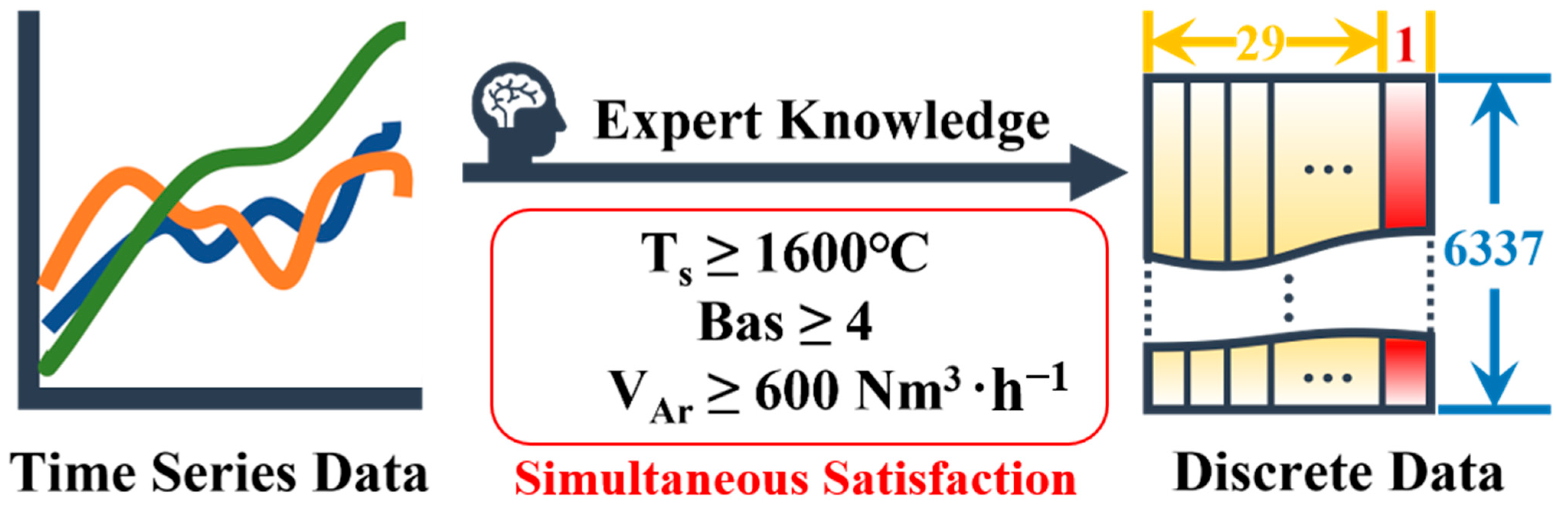
Based on the reaction $\Delta G^{\Phi }$, it is known that the desulfurization reaction proceeds normally under conditions where the slag basicity is high, the temperature is high, the aluminum content in the steel is high, and the dissolved oxygen content is below a certain threshold. According to the expert knowledge provided by metallurgical process engineers, the following conditions are considered necessary for the desulfurization reaction in actual production: the steel temperature should not be lower than 1600 °C, the basicity should not be lower than 4, and the argon blowing flow rate should not be lower than 600 Nm³·h⁻¹.

In addition to thermodynamic equilibrium, the desulphurisation process in the LF is strongly governed by kinetic factors. The overall reaction rate is typically controlled by a combination of mass transfer in the molten steel and slag phases, as well as the interfacial chemical reaction between slag and metal. Argon stirring plays a crucial role in enhancing mixing and increasing the effective slag–metal contact area, thereby accelerating sulphur removal.

The efficiency of desulphurisation is therefore influenced not only by equilibrium conditions such as temperature and slag basicity but also by dynamic process variables including stirring intensity, refining time, and slag fluidity. These coupled thermodynamic–kinetic effects have been widely discussed in previous studies on LF refining. For example, Kargul and Falkus (2010) [25] proposed a hybrid model that integrates thermodynamic equilibrium with kinetic transport phenomena, highlighting the importance of process conditions in determining sulphur removal efficiency.

In this study, although an explicit kinetic model is not implemented, the key process variables that reflect both thermodynamic and kinetic effects are incorporated into the machine learning framework, enabling a data-driven representation of the underlying metallurgical mechanisms.

2.2. Overall Modelling Workflow

The overall workflow of the proposed hybrid modelling framework is summarised as follows. First, industrial process data corresponding to high-purity iron and non-alloy steel heats since August 2022 are extracted from the L2 process control system of a steel plant. The time window is defined as the period during which the refining conditions (e.g., temperature, basicity, and argon flow rate) are simultaneously satisfied. For each heat, the representative values of the process variables are obtained by averaging the data within the selected time window. Second, missing values, outliers and unit inconsistencies are treated using a combination of deletion, statistical imputation and unit conversion, after which 5169 heats with 29 independent variables and one dependent variable (endpoint sulphur content) remain. Third, all features are scaled to the interval (0, 1) using Min–Max normalisation, and highly collinear variables are removed based on a Pearson correlation heatmap, resulting in a reduced feature set that retains the most informative process descriptors. Fourth, K-means clustering is applied in the original feature space to group the multi-grade heats into representative operating modes, while principal component analysis (PCA) is used only to visualise the clustering results in a three-dimensional space; for subsequent modelling, the cluster corresponding to low-sulphur, high-purity grades is selected as the primary dataset. Finally, four ML models—RF, XGBoost, SVM and ANN—are trained and evaluated on this cluster using a uniform train–test split and cross-validation scheme. The best-performing model is further tuned and interpreted using SHAP to elucidate the roles of key process variables in controlling endpoint sulphur. The detailed steps of data preprocessing, clustering, feature engineering and model construction are described in Section 2.3 and Section 3.

All computations in this study were carried out using Python 3.10 on a workstation equipped with an Intel Xeon W-2245 CPU (3.90 GHz) and 64 GB of RAM. Data handling and visualisation were performed with NumPy (version 1.24), pandas (version 2.0) and Matplotlib (version 3.7). The machine learning models were implemented using scikit-learn (version 1.3) for RF, SVM and K-means clustering; XGBoost (version 1.7) for the gradient-boosting model; and TensorFlow (version 2.12) for the ANN. SHAP was computed using the SHAP library (version 0.43).

To ensure reproducibility and a fair comparison of the candidate models, a fixed random seed was used throughout the workflow. The train–test split, K-means initialisation, cross-validation shuffling and random components of the RF, XGBoost, SVM and ANN models were all controlled by setting random_state = 42 in the corresponding functions. The same data partitioning and cross-validation folds were applied to all four models, so that the performance differences reported in Section 3.2 arise solely from the model structures and hyperparameters rather than from differences in data sampling or random initialisation. Further details of the preprocessing and modelling scripts are provided in the accompanying GitHub (commit ID: 2a4096a) repository described in the Code Availability section.

2.3. Data Collection and Preprocessing

In this study, all data were obtained from the L2 process control system of a large steel plant. The L2 system continuously records time series information on molten steel composition, slag additions, alloy additions, electrical energy input and argon stirring throughout LF refining [26]. For the purpose of modelling LF desulphurisation, heats corresponding to high-purity iron and non-alloy steels produced since August 2022 were selected, and the relevant L2 records were exported for further processing. Because the L2 data are inherently time series and cannot be used directly in standard machine learning algorithms [27], they must be discretised into representative samples that capture the key conditions of the desulphurisation stage. This single-sample representation inevitably removes the detailed early–middle–late evolution within the desulphurisation window; however, it provides a robust and consistent set of features for an initial comparison of alternative machine learning models on heterogeneous industrial data with irregular sampling intervals and occasional gaps in the L2 records. Consequently, sequence-based models such as LSTM or ARIMA were not considered in the present study, but remain a worthwhile direction for future work.

Guided by metallurgical expert knowledge, a heat was regarded as valid for desulphurisation modelling if, during its LF refining stage, there existed at least one period in which the following three refining conditions were simultaneously satisfied: steel temperature ≥1600 °C, slag basicity ≥4 and argon-blowing rate ≥600 Nm³·h⁻¹. Heats that never met this combination of conditions were excluded from the dataset. For each retained heat, the LF refining record as a whole was treated as one machine learning sample, that is, the presence of a desulphurisation stage in the LF process rendered the corresponding heat a valid sample. In this way, each heat contributes exactly one sample, and an initial dataset comprising 6337 records with 29 quantitative independent variables and one dependent variable (endpoint sulphur content) was established, as illustrated schematically in Figure 2.

It is widely acknowledged that data quality fundamentally constrains the predictive performance of ML models. Industrial datasets often contain various forms of noise—including missing values, outliers, inconsistent measurement units, and irrelevant information—that can distort model learning and reduce accuracy. Proper data cleaning and denoising procedures are therefore indispensable to enhance the overall signal-to-noise ratio and ensure the reliability of the resulting model.

2.3.1. Handling Missing Values

In practical industrial datasets, the presence of missing values is inevitable. These omissions may originate from multiple sources, including manual recording errors during data acquisition, temporary sensor malfunctions, or time delays inherent to real-time process control in L2 steelmaking systems. Furthermore, some null entries arise naturally due to the absence of specific process operations, for example, when a particular additive is not introduced during a given LF cycle, resulting in a structurally missing variable.

Given the heterogeneous nature of missing data in industrial process records, missing values were handled according to their underlying causes rather than by using a uniform strategy. When missingness directly affected the target variable, i.e., the LF endpoint sulphur content, the corresponding samples were removed, since their inclusion would compromise model training and prediction accuracy.

For missing values in input features that were not directly related to the prediction target, mean imputation was adopted to preserve data integrity and maximise sample utilisation while maintaining overall distributional consistency. In addition, for process-specific variables such as material additions, zero values were retained when they represented actual operating conditions rather than missing records.

2.3.2. Handling Outliers

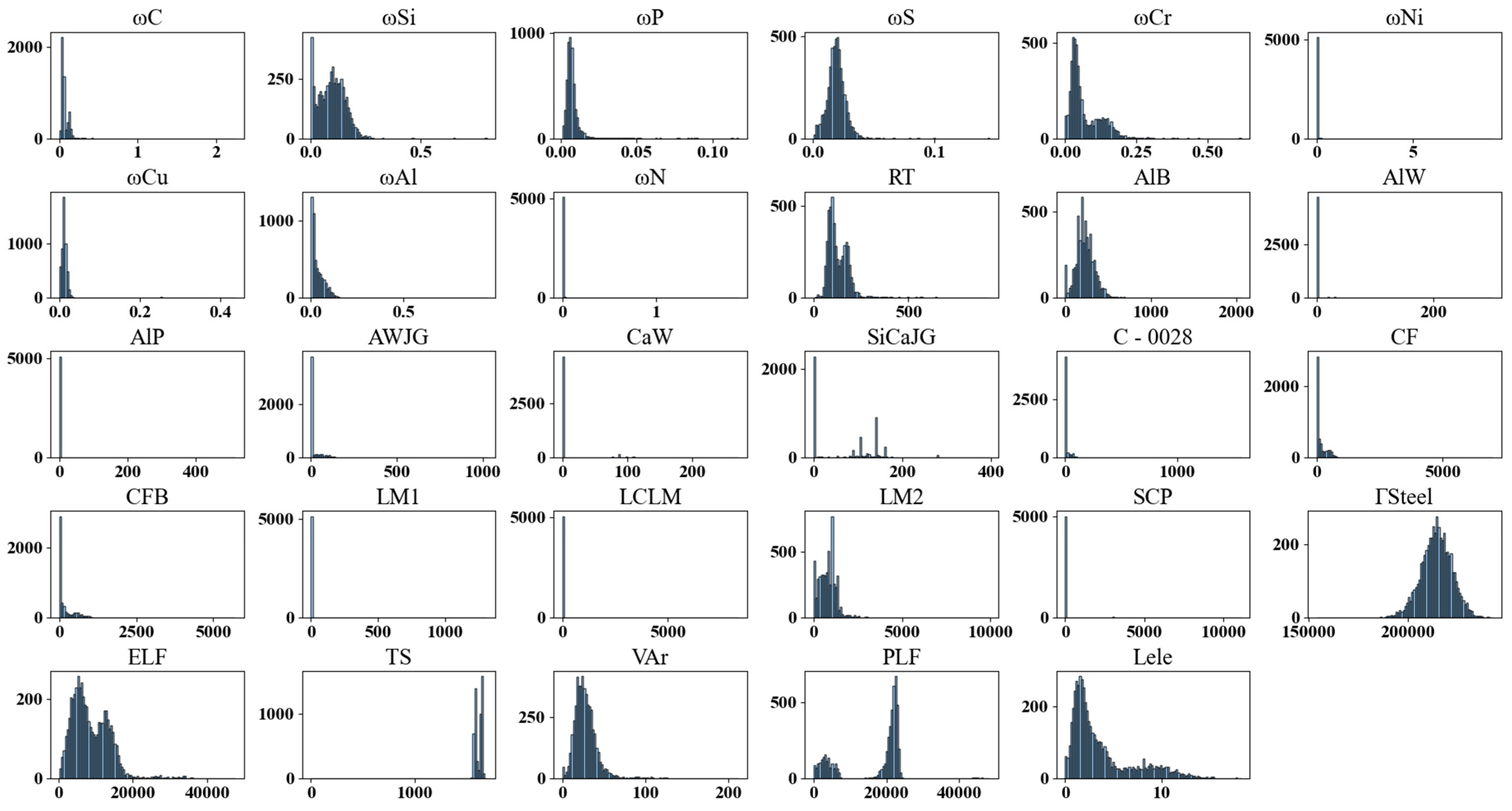
In general, performing a distribution analysis on the data can effectively identify outliers. First, a histogram of the data distribution is plotted, as shown in Figure 3. The Pauta criterion (3σ) is then used to remove outliers that deviate significantly from the mean. The principle behind this method assumes that the errors in the data samples are purely random errors. It involves calculating the arithmetic mean $\mu$ of all samples $x_1$, $x_2$, …, $x_n$; the residual error ${\upsilon }_i$; and the standard deviation $\sigma$. The residual error is then compared to 3σ using the following Equation (6) to determine whether the sample should be deleted:

$$\left|{\upsilon }_i\right|=\left|x_i-\mu \right|>3\sigma$$

(6)

In this study, the 3σ criterion was adopted as an empirical approach for preliminary outlier screening in industrial process data, rather than being under the strict assumption of normality. Although some variables deviate from Gaussian distributions, this method remains effective for identifying extreme abnormal values. Data points beyond ±3σ were therefore flagged and further examined within each steel grade or cluster. Only those associated with clear measurement errors or inconsistent process records were removed, while metallurgically reasonable extreme values were retained.

It is important to note that some outliers are caused by changes in the unit standards of the L2 process control system during the production cycle, such as the change in the unit of V_Ar from NL to Nm³. These can be resolved by converting the units accordingly. In addition, several variables exhibit skewed distributions. No further transformation (e.g., log or Box–Cox) was applied, as the selected models are relatively robust to such distributional characteristics and retaining the original variable scale facilitates metallurgical interpretation. After handling the missing values and outliers, the total sample size in the dataset decreased from 6337 to 5169, with the number of features remaining unchanged at 29 independent variables and 1 dependent variable.

2.3.3. Data Standardization

Even after the removal of outliers, inconsistencies in measurement units and feature scales persist within the dataset. For certain algorithms—such as SVM and ANN—the comparability of feature magnitudes is a prerequisite for effective learning. In these models, distance- or gradient-based optimisation depends on the relative numerical scale of input features. However, the variables within metallurgical datasets often differ substantially in both units and ranges. For instance, in the LF refining dataset constructed in this study, elemental concentrations typically vary between 0 and 1 wt%, whereas the molten steel mass can exceed 200,000 kg. Without scaling, features with larger numerical magnitudes dominate the optimisation process, resulting in biased model fitting and an inaccurate assessment of feature importance.

To eliminate such scale disparities and ensure that all features contribute comparably to model training, Min–Max normalisation was applied. Specifically, the MinMaxScaler function from sklearn.preprocessing (feature_range = (0, 1)) was used to linearly transform each feature into the interval (0, 1) according to Equation (7):

$$x^{\prime }={\displaystyle \frac{x-x_{min}}{x_{max}-x_{min}}}$$

(7)

where $x$ is the original feature value; $x_{min}$ and $x_{max}$ denote the minimum and maximum values of the feature, respectively; and $x^{\prime }$ represents the normalized value. Through this transformation, all variables are brought onto a uniform scale, ensuring that large-magnitude features do not overshadow those with smaller numerical ranges and allowing the learning algorithm to capture the true physical relationships among process variables.

2.3.4. K-Means Algorithm for Sample Classification with Metallurgical Expert Knowledge

The samples in the dataset come from the smelting results of different steel grades. Among the 5169 samples, there are 126 distinct steel grades. These grades have different requirements for impurity element control. Some require low carbon, low sulfur, and low phosphorus, such as the raw material pure iron FS3-8; others require high carbon and low aluminum and titanium, such as pipeline steel X42-2; while some, like carbon steel Q355B-AY, have less stringent impurity content requirements. The desulfurization processes for different steel grades are also varied. If these are mixed together for model training, the data will interfere with each other, reducing the overall accuracy and interpretability of the model.

This study primarily uses K-Means clustering analysis based on centroid calculations, an exploratory data analysis method. Unlike discriminant analysis, clustering analysis does not require prior knowledge of category standards or the number of categories before classification. It automatically classifies sample data based on feature characteristics, thereby revealing the underlying structure in the data. The data is projected onto a three-principal component vector space using PCA, where n_components = 3 is chosen for easy and intuitive visualization of the relationships between data samples. The kmeans.fit() function is then applied to divide the data samples into multiple clusters, with data points in each cluster being highly similar and treated as the same category for model training.

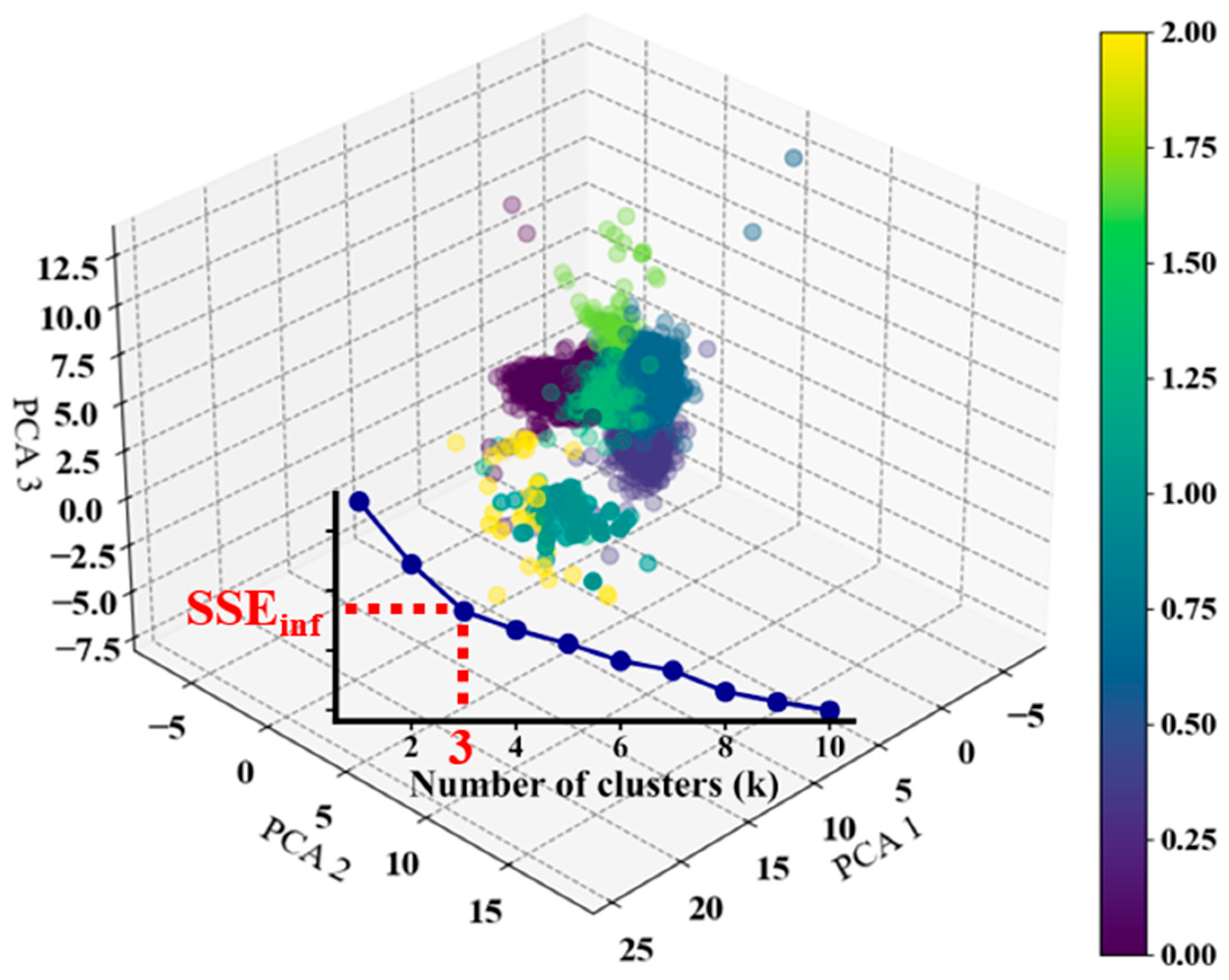
The Elbow Method is a heuristic approach used to select the optimal number of clusters $k$ in K-Means clustering. Its principle is based on the Sum of Squared Errors (SSE), also known as the within-cluster sum of squares or inertia, which measures the Euclidean distance from data points to their respective cluster centroids. In other words, it calculates the sum of squared distances from data points to the centroid of their assigned cluster. The formula is presented in Equation (8):

$$SSE=\sum _{i=1}^n\sum _{x\in C_i}{‖x-{\mu }_i‖}^2$$

(8)

where: $C_i$ is the $i$-th cluster, ${\mu }_i$ is the centroid of $C_i$, and $x$ is a data point.

As the number of clusters $n$ increases, the SSE typically decreases because with more clusters, each cluster contains fewer data points, and the distance between the centroid and the data points becomes smaller. When the number of clusters is very small (e.g., $n=1$), all data points are assigned to a single cluster, resulting in a very high SSE. As $n$ increases, the data points are better partitioned into their respective clusters, and the distance between centroids and data points decreases, causing the SSE to drop rapidly. However, once $n$ reaches a certain point, the data points within each cluster become sparse, and the rate of decrease in SSE slows down. This situation is reflected by an inflection point in the curve at [$k$, ${SSE}_{inf}$], as shown in Figure 4. At this point, increasing the number of clusters further no longer significantly improves the clustering result. The elbow method suggests that $n=k$ is a reasonable choice.

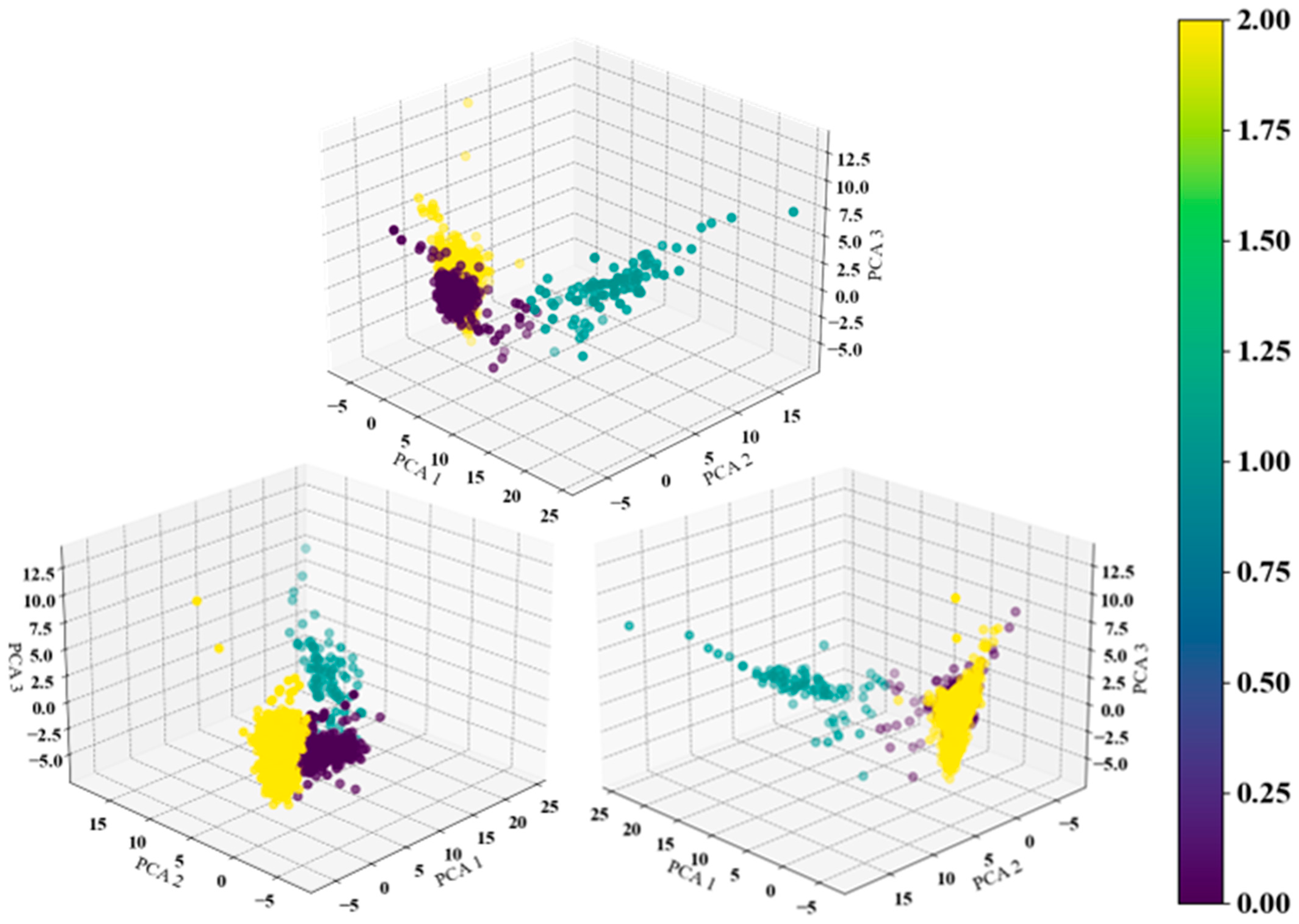
Through iterative computation and evaluation, the optimal clustering performance was obtained when the number of clusters k = 3. The clustering visualization corresponding to $n=3$ is presented in Figure 5. According to metallurgical domain knowledge, after excluding steel grades that do not undergo the desulfurization process, the remaining grades can be logically categorized into three distinct groups. The K-means clustering results exhibit a high degree of consistency with this expert-driven classification, confirming the rationality of the algorithmic partition. The corresponding classification outcomes are summarized in

Table 2. Steel grade classification results.

Classification	Quantity	Type of Steel
1st class	7	FS3-1, FS3-10, FS3-11, FS3-16, FS3-5, FS3-7A, FS3-8
2nd class	30	L245, LX52-1, T700, T700L, T700L-1, T700L-2, T700QZ, T750L, X42, X42-1, X42-2, X42-3, X46-1, X52-1, X52-2, X52-5, X52MS-1, X52MS-5, X60-2, X60-3, X60-6, X60-7, X60-9, X65-5, X65-6, X65-8, X70-2, X70-5, X70-6, X70-8
3rd class	67	15CrMoR, 16MnDR, 252086, 253223, 261252, 262209, 30CrMnSiA, 30MnB5, 35Si2MnCrMoV, 73Ni8, 750TM175, ASME SA-765 Gr4, C22.8L, C45, C60, DL510, FAS500L-Z, FAS355L-Z, FAS500L-Z, HP295, HP325, L907A-1, L907A-2, LQ235-1, LQ355-1, LQ460-1, Q345B, Q345NQR2, Q345q-1, Q345q-2, Q345qD, Q345qD(roll), Q345RT-1, Q345RT-2, Q345RT-3, Q355-3, Q355-4, Q355-6, Q355C(Si + P), Q355B-AY, Q355T-1, Q420M, Q450NQR1, Q450NQR1-2, QStE420TM, S355J0-2, S355JR-1, S355MC-3, S700MC-M, T330CL, T400CL, T510L, T520JJ, T610L, TATM700, TQ340-1, TQ345, TQ420-4, TQ460MC-1, TQ460MC-2, TQ550MC-3, TQ600MCC, TQ600MCC/TQ600MCD, TQ600MCC-1, TQ700MC-1, TQ700MC-2, (null)
Unclassified steel grades	22	10, 20, MR T2.5, MR T3, Q195, Q195L, Q195-W, Q195-Delong, Q235-1, Q235-2, Q235B-YT, Q235B-Zhong, Q235-DL, Q245RT, S235JRG2, S235JRG2-2, S275JR-1, SA414-G, SN400B-2, SS400, SS400-1, SS400FL

. After clustering, cluster 1, which mainly contains high-purity iron and low-alloy steel heats under relatively stable operating conditions, was selected as the representative dataset for subsequent modelling. Unless otherwise stated, all model training and performance metrics reported in Section 3 refer to this cluster.

The investigated dataset covers a range of steel categories commonly produced in industrial practice, including carbon steels, pipeline steels, and high-purity iron grades. Carbon steels are primarily characterised by their carbon content and are widely used in structural applications, while pipeline steels (e.g., X65, X70, X80) are designed with controlled compositions to achieve high strength and toughness for oil and gas transportation. High-purity iron grades are typically produced under stringent refining conditions with very low impurity levels.

In general, the chemical composition of these steels involves varying levels of elements such as C, Si, Mn, P, S, and trace alloying elements (e.g., Ni, Cr, Mo), which influence both thermodynamic equilibrium and kinetic behaviour during the desulphurisation process. The inclusion of multiple steel types in this study enhances the robustness and generalisability of the proposed machine learning model. The classification of steel grades follows commonly accepted industrial standards.

3. Results and Discussion

3.1. Feature Engineering

Once the dataset is established, the raw data must be refined to align with the research objectives through a process commonly referred to as feature engineering. The essence of feature engineering lies in identifying and transforming variables to retain features that meaningfully contribute to the predictive target while removing redundant or irrelevant attributes. By constructing an optimal subset of informative features, the model can better capture the intrinsic structure of the data and improve its generalization capability. This step is pivotal in determining the upper limit of model performance, as improper feature selection often constrains both the interpretability and predictive accuracy of the algorithm.

Accordingly, the design and selection of feature groups in the LF refining process were guided by metallurgical principles to ensure that each feature reflects the physical and chemical mechanisms governing desulfurization. This knowledge-driven approach enhances both the interpretability and predictive precision of the ML model. The complete list of features employed as independent variables in this study is summarized in

Table 3. Summary of Independent Variables Features.

Features	Description	Unit	Range	Mean
ωC	Carbon content after the converter	wt%	0.0036~2.24	0.0677
ωSi	Silicon content after the converter	wt%	0.0007~0.7923	0.0951
ωP	P content after the converter	wt%	0.001~0.117	0.0076
ωS	S content after the converter	wt%	0.000818~0.1456	0.0192
ωCr	Cr content after the converter	wt%	0.00001~0.6121	0.0672
ωNi	Ni content after the converter	wt%	0.000167~9.1058	0.0209
ωCu	Cu content after the converter	wt%	0.000083~0.4325	0.0159
ωAl	Al content after the converter	wt%	0.000001~0.9479	0.0378
ωN	N content after the converter	wt%	0.000084~1.8534	0.0043
RT	Refining time of LF process	min	12.6~927.9	135.15
AlB	The amount of aluminum pellet	kg	0~2056	232.86
AlW	aluminum wire	kg	0~300	3.4433
AlP	aluminum particles	kg	0~510	3.5190
AWJG	aluminum wire JG	kg	0~1021	28.283
CaW	Calcium wire	kg	0~270.82	8.3688
SiCaJG	Calcium Silicon wire	kg	0~396	70.255
C-0028	Coal-based carburizer	kg	0~1571	13.670
CF	Fluorite	kg	0~6983	201.33
CFB	Fluorite Ball	kg	0~5717	197.38
LM1	Limestone 1#	kg	0~1294	2.7955
LCLM	Externally purchased limestone	kg	0~8332	97.486
LM2	Limestone 2#	kg	0~9956	794.86
SCP	Recycled scrap	kg	0~11,091	58.467
ΓSteel	Weight of molten steel in ladle refining	kg	154,165~242,121	214,016
ELF	Total power transmission of LF process	kW·h	294~47,605	8747.5
TS	Tapping temperature at the end of LF process	°C	1311~1689	1609.7
VAr	LF furnace bottom blowing argon flow rate	Nm3·h−1	0~12,720	1711.74
PLF	LF furnace power supply	kW	0~48,328	16,517
Lele	Consumption of Graphite electrode	kg	0~18.263	3.7249

.

When two or more features in the dataset exhibit a high degree of correlation, it becomes difficult for the model to determine the independent contribution of each feature to the target variable. These features provide redundant information, which leads to instability in the model’s coefficients (weights). This situation can cause significant fluctuations or even cancellation effects between the features, and minor noise or changes in the data can lead to large changes in the model parameters. This phenomenon is known as multicollinearity. Multicollinearity makes it difficult for the model to accurately interpret the independent impact of each feature on the target variable. For example, in a regression model, if two features are highly correlated, the model cannot distinguish their individual contributions, which compromises the interpretability of the analysis. It also increases the standard errors of parameter estimates in the regression model, making statistical significance tests (e.g., $p$-values) unreliable. As a result, even if some features are indeed related to the target variable, the model may incorrectly deem their effects insignificant. This situation can lead to model overfitting and adversely impact the model’s generalization ability.

The Pearson correlation coefficient (denoted as $r$) is a statistical measure used to assess the linear relationship between two variables. Its value ranges from −1 to 1, indicating the strength and direction of the linear relationship between the variables. For two variables X and Y, the formula for the Pearson correlation coefficient is defined by Equation (9):

$$r={\displaystyle \frac{Cov\left(X,Y\right)}{{\sigma }_X{\sigma }_Y}}$$

(9)

where $Cov(X,Y)$ is the covariance between variables $X$ and $Y$, representing the direction and degree of their linear relationship; ${\sigma }_X$ and ${\sigma }_Y$ are the standard deviations of $X$ and $Y$, respectively, used to measure the dispersion of the data.

The formula can be expanded as shown in Equation (10):

$$r={\displaystyle \frac{{\sum }_{i=1}^n{(X}_i-\overline{X}){(Y}_i-\overline{Y})}{\sqrt{{\sum }_{i=1}^n{{(X}_i-\overline{X})}^2}\sqrt{{\sum }_{i=1}^n{{(Y}_i-\overline{Y})}^2}}}$$

(10)

where $X_i$ and $Y_i$ are the $i$-th sample value of variables $X$ and $Y$; $\overline{X}$ and $\overline{Y}$ are the mean values of variables $X$ and $Y.$

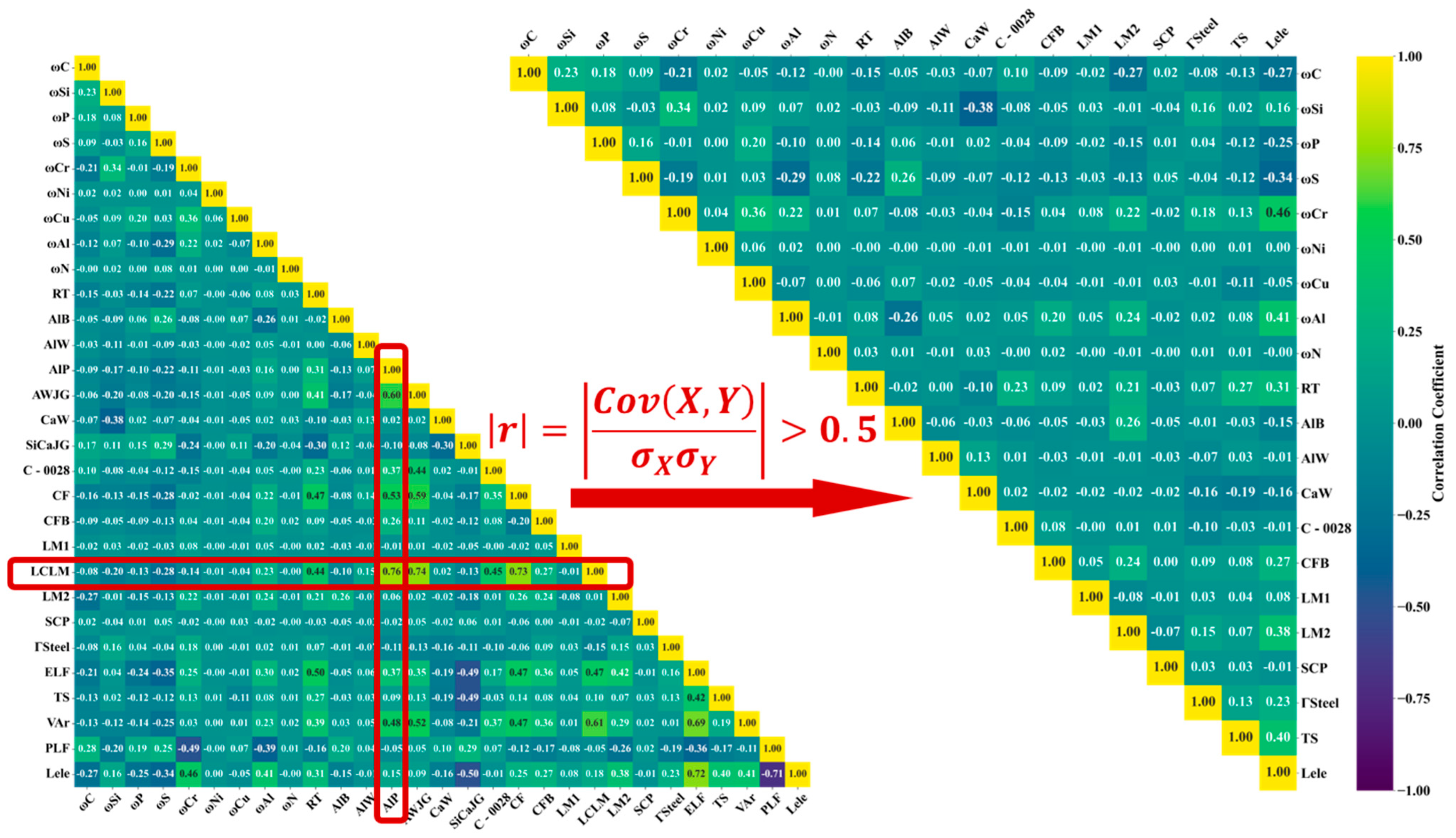
When the correlation coefficient $r=1$, this indicates that $X$ and $Y$ are perfectly positively linearly correlated. When $r=-1$, this indicates that $X$ and $Y$ are perfectly negatively linearly correlated. When $r=0$, this indicates that there is no linear correlation between $X$ and $Y$. Based on this criterion, the correlation matrix is calculated using the np.corrcoef() method. Additionally, a heatmap of the Pearson correlation coefficients between the features is plotted using sns.heatmap(), with an appropriate threshold set. In this study, a correlation threshold of $\mid r\mid >0.5$ was adopted as a practical criterion to reduce redundancy among highly correlated variables while retaining sufficient process information. This threshold provides a balance between feature simplification and information preservation, which is beneficial for both model performance and interpretability. Features with a correlation exceeding this threshold are removed. After performing dimensionality reduction through correlation analysis, the dataset’s dimensions are reduced from 29 to 21, as shown in Figure 6.

From the perspective of metallurgical expert knowledge, the reasons for the strong correlation between these features are as follows: Aluminum pellets AlP serve as deoxidizers, and their function highly overlaps with that of aluminum wire AWJG, resulting in a high correlation coefficient. The addition of aluminum as a deoxidizer creates the necessary reducing conditions for desulfurization, while the subsequent addition of externally purchased limestone LCLM serves the purpose of desulfurization, making the objectives of these two processes consistent. As a result, their correlation coefficient is high in the data. Similarly, fluorspar CF is used to lower the steel slag melting point, improve slag fluidity, and promote the exchange of materials between steel slag and molten steel, thereby enhancing the desulfurization effect. The amount of CF added is determined by the slag quantity, which is influenced by the addition of slag-forming agents like limestone. Therefore, the correlation coefficient between CF and LCLM is high. The total electrical power input ELF, argon blowing amount VAr, and LF power input PLF are all necessary conditions for the desulfurization reaction, with similar functions, leading to a high correlation coefficient as well.

3.2. Model Selection and Construction

Four representative machine learning models—RF, XGBoost, SVM and ANN—were employed to model the preprocessed desulphurisation dataset. After data cleaning, normalisation and clustering, the selected cluster was randomly partitioned into a training set (90% of the heats) and a test set (10% of the heats). The dataset was randomly divided into training and test sets at a ratio of 9:1. Given the relatively large sample size, this setting provides enough data for model training while maintaining a representative test set for evaluation.

Each model was first fitted and tuned on the training set using 10-fold cross-validation and then retrained with the optimal hyperparameters on the full training set. The held-out test set was finally used to compare the generalisation performance of the four models in terms of the R², RMSE and MAE for endpoint sulphur content. Based on these metrics, the most suitable model for the desulphurisation system was identified and subsequently used for in-depth optimisation and interpretability analysis.

In practical LF production, model performance is often assessed using the hit rate (HR) within a specified error tolerance, since this metric is directly related to whether the predicted endpoint sulphur content satisfies process control requirements. In this study, a relatively strict tolerance range of ±0.0025 wt% was adopted for HR evaluation [4]. In addition, scatter plots of measured versus predicted sulphur content for both the training and test sets were constructed to visualise the correspondence between predictions and observations and reveal any systematic bias or heteroscedasticity. Through this combination of quantitative error metrics, tolerance-based accuracy and graphical analysis, the overall predictive capability and stability of the four models were systematically compared.

3.2.1. Random Forest (RF)

RF is an ensemble learning algorithm based on decision tree models, widely used in regression and classification tasks. In materials science, it is commonly applied in tasks such as assisting in the design of alloy compositions, which are difficult to accomplish manually. Compared to a single decision tree model, RF combines multiple simple estimators, making it more robust and resistant to interference.

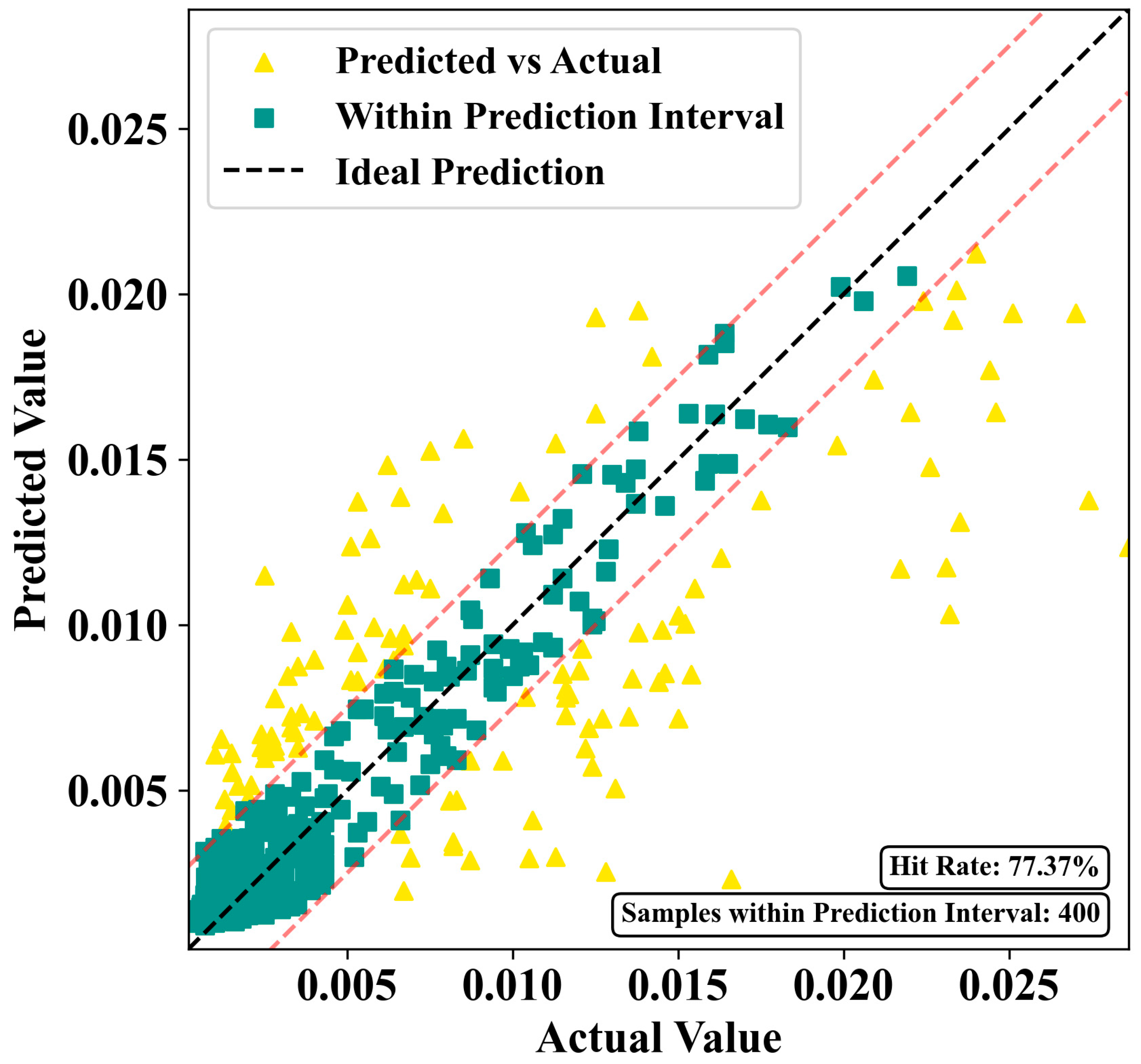
In this study, the RF model parameters are set as: n_estimators = 500, max_depth = 20, min_samples_split = 10, min_samples_leaf = 5, max_features = 0.1, with a cross-validation fold (cv) of 10. On the test set, 77.37% of heats have an absolute prediction error within ±0.0025 wt% for sulphur, which is used as the HR indicator for this study. The results are shown in Figure 7.

3.2.2. Extreme Gradient Boosting (XGBoost)

XGBoost is an efficient ML algorithm based on the gradient boosting method. It is widely applied to various supervised learning tasks, such as classification and regression. The core idea is to build multiple weak learners (typically decision trees) and chain them together, with each round of the model learning the residuals (i.e., the errors between predicted and true values) based on the results of the previous round. By gradually reducing the residuals, XGBoost improves overall prediction accuracy. This algorithm has performed excellently in numerous ML competitions and is widely recognized for its computational efficiency and flexibility. It is also robust to data distribution and particularly suitable for handling imbalanced or discrete datasets.

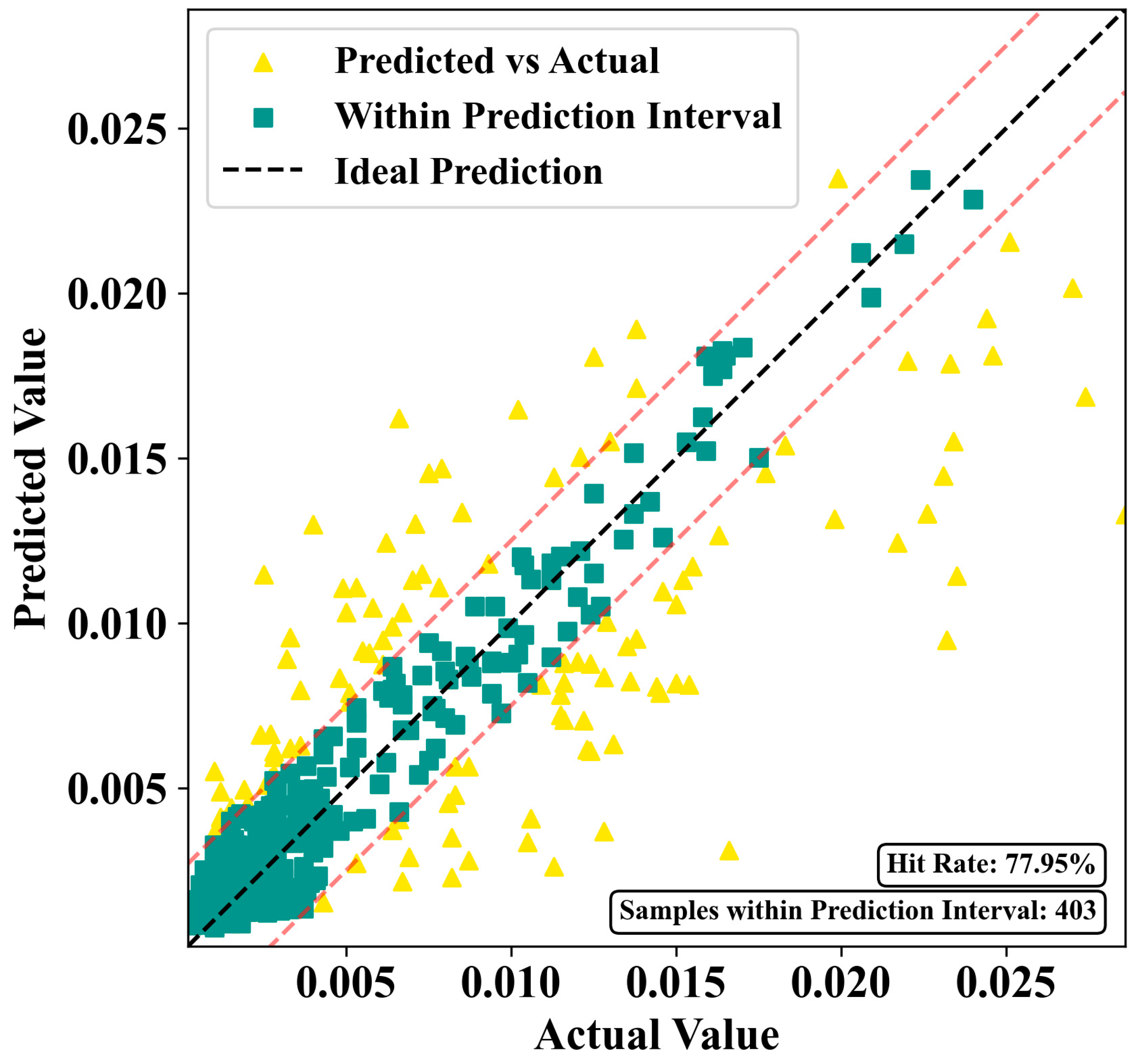
In this study, the XGBoost model parameters are set as follows: max_depth = 10, eta = 0.05, objective = ‘reg:squarederror’, eval_metric = ‘rmse’, subsample = 0.8, colsample_bytree = 0.8, alpha = 0.1, lambda = 1, with 10-fold cross-validation (cv = 10). On the test set, 77.95% of heats fall within ±0.0025 wt% absolute error in sulphur prediction, corresponding to the HR metric for this model. The results are shown in Figure 8.

3.2.3. Support Vector Machine (SVM)

In this work, support vector regression (SVR) is adopted rather than the original binary classification formulation of an SVM. SVR seeks a regression function that minimises a regularised ε-insensitive loss, which allows it to control both the flatness of the function and the magnitude of prediction errors. By introducing a kernel function, the input variables are implicitly mapped into a higher-dimensional feature space, so that a linear relationship in the feature space corresponds to a nonlinear relationship between the process variables and endpoint sulphur content.

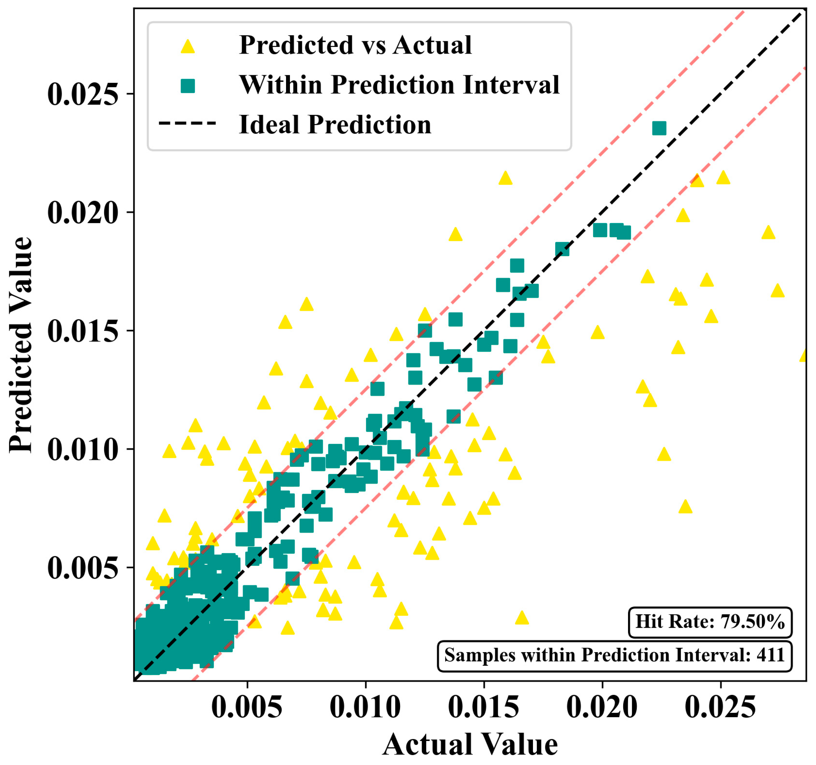
In this study, the SVM model parameters are set as follows: C = 1, epsilon = 0.2, gamma = ‘scale’, kernel = ‘rbf’, tol = 1 × 10⁻⁴, with 10-fold cross-validation (cv = 10). For the SVM model, 77.95% of heats exhibit an absolute prediction error within ±0.0025 wt% for sulphur on the test set, yielding an HR comparable to that of the tree-based models. The results are shown in Figure 9.

3.2.4. Artificial Neural Network (ANN)

ANN is a computational model that simulates the biological neural system, primarily used for solving pattern recognition, regression, classification, and other problems. ANN processes information through a hierarchical structure of neurons, with each neuron simulating the function of a biological neuron. Neurons can be activated by activation functions and transmit information through connection weights.

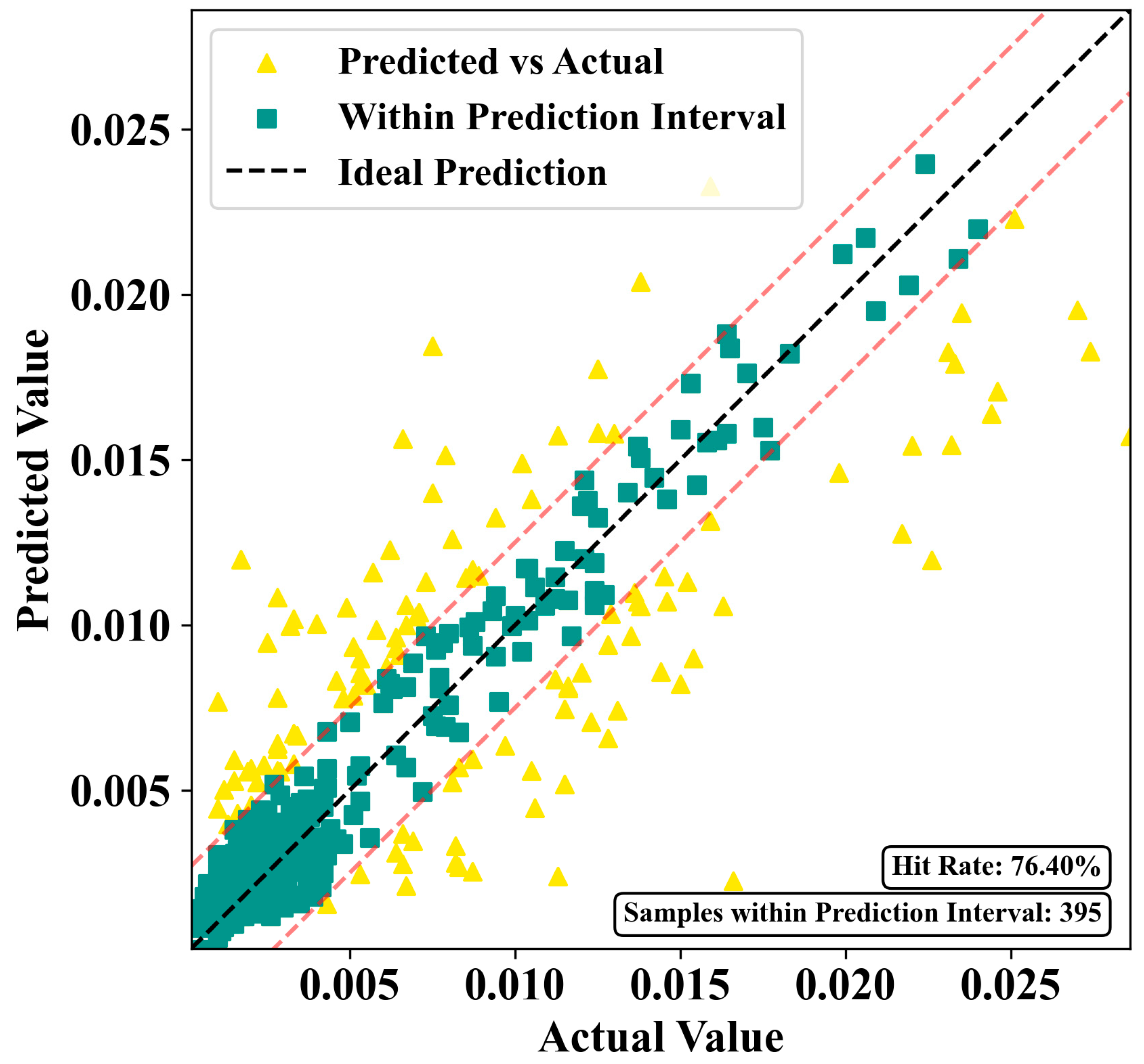
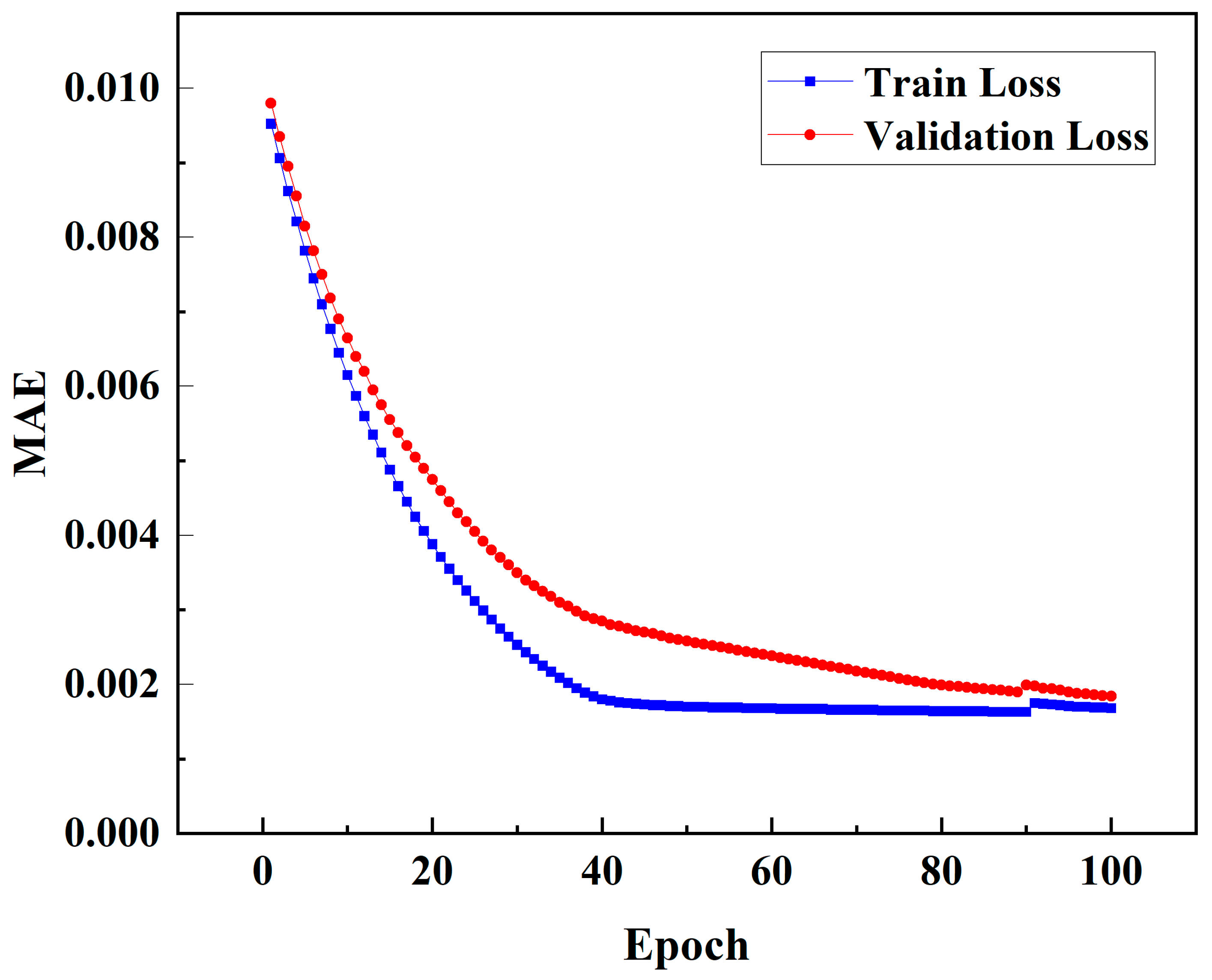
The NN model in this study is constructed with one fully connected layer as the input layer, two hidden layers with 128 and 64 neurons respectively, and two Dropout() layers for regularization. The model used the ReLU activation function and was trained using the Adam optimizer with a learning rate of 0.001. The MAE was adopted as the loss function. The training process was conducted for 100 epochs with a batch size of 128 and a validation split of 0.1. For the ANN model, 76.40% of heats in the test set have an absolute prediction error within ±0.0025 wt% for sulphur, indicating a comparable HR with slightly better error metrics than the other models. The results are shown in Figure 10.

The corresponding training and validation loss curves are presented in Figure 11 to illustrate the convergence behaviour of the model during training.

3.2.5. Selection of the Optimal Model

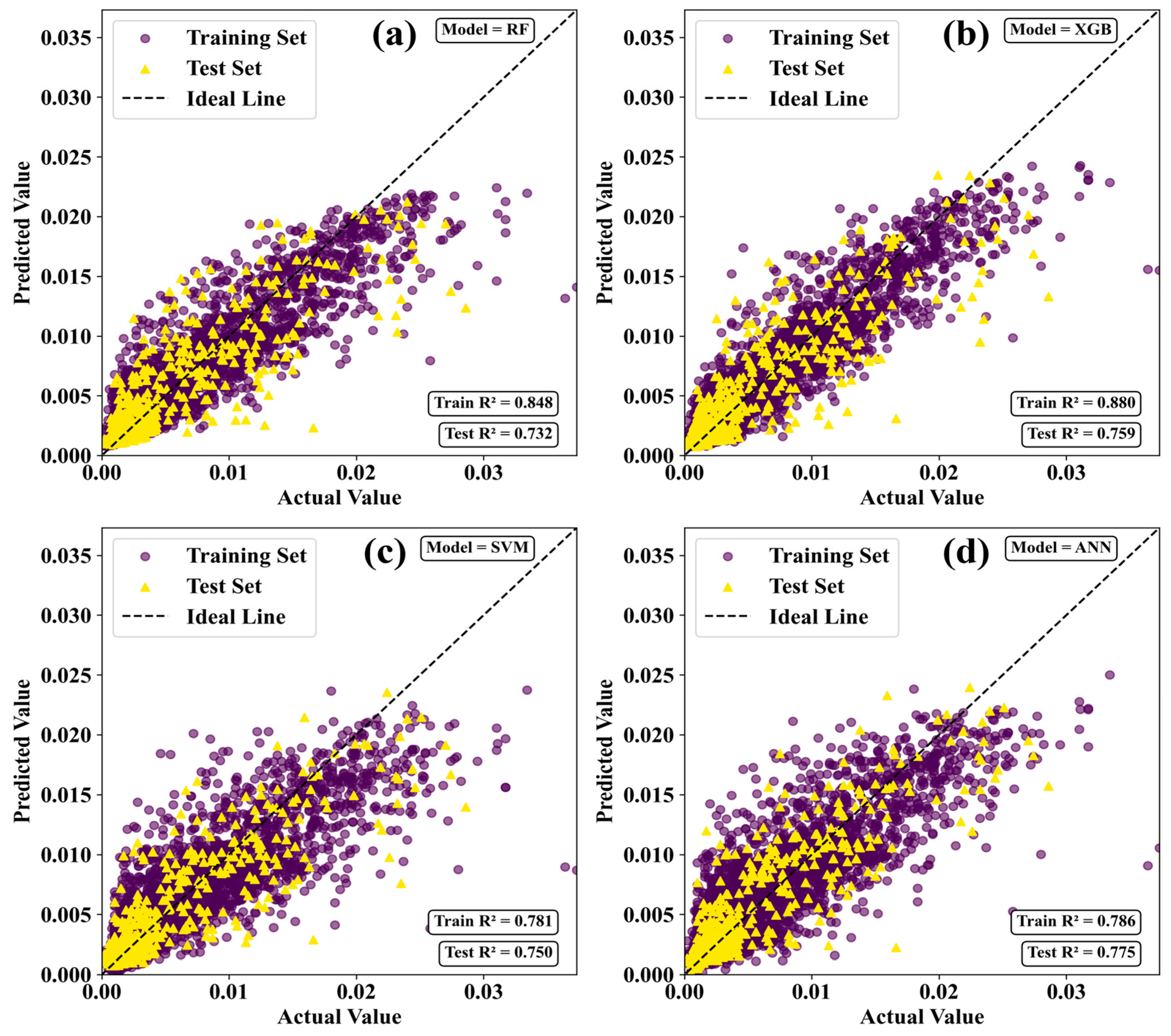
Four models are used to predict the desulfurization data, and the data distribution scatter plot is generated. As shown in Figure 12, in this application scenario, the RF model and XGBoost model show some tendency to overfit (with a significantly higher R² for the training set compared to the test set). It is analyzed that these two models, based on tree structures, are more suitable for classification tasks and tend to overfit when applied to regression problems due to the influence of data partitioning. In contrast, the SVM model and ANN model show R² values that are closer between the training set and test set, and no overfitting is observed.

Table 4. Comparison of Performance Metrics for Four Models.

Model	Evaluation Indexes
	R2	RMSE	MAE	HR	Runtime
RF	0.7321	0.0029	0.0018	77.37%	1.7 s
XGBoost	0.7589	0.0028	0.0017	77.95%	2.1 s
SVM	0.7498	0.0028	0.0017	79.50%	0.8 s
ANN	0.7752	0.0027	0.0017	76.40%	0.4 s

presents the detailed performance metrics of the four models on the test dataset, including the R², RMSE, MAE, HR and runtime. Here, HR denotes the percentage of heats in the test set whose absolute prediction error for endpoint sulphur lies within ±0.0025 wt% S, which corresponds to the sulphur specification tolerance (approximately 25 ppm) used in the studied plant. Comparative analysis reveals that the ANN model achieved the highest predictive accuracy, with an R² value of 0.7752. Although this value may appear moderate, it is considered acceptable for industrial LF processes, where endpoint sulphur prediction is influenced by complex thermodynamic–kinetic interactions, operational variability, and measurement uncertainty. Simultaneously, the ANN model exhibited the lowest RMSE (0.0027) and MAE (0.0017), reflecting superior precision and minimal prediction deviation.

In practical applications, model performance is commonly evaluated using the HR within a specified error tolerance, rather than relying solely on R². In this study, a relatively strict tolerance range was adopted, and the model achieved a high hit rate under this criterion, demonstrating its effectiveness in meeting industrial requirements. In addition, the model is trained on a large and heterogeneous dataset covering multiple steel grades and refining conditions, which further increases the prediction difficulty. Therefore, the obtained performance is considered reasonable and practically applicable.

Furthermore, compared with previous studies on similar metallurgical prediction problems, the performance of the proposed model is within a comparable range [24,28]. Since the endpoint sulphur prediction problem involves strongly nonlinear interactions among process variables, the present study focused on representative nonlinear models. Nevertheless, the inclusion of simpler baseline models such as linear regression could provide additional reference and will be considered in future work.

3.3. Model Tuning and Interpretation

The process of validating and optimizing the ANN model primarily involves assessing model performance, diagnosing potential overfitting or underfitting issues, and selecting appropriate hyperparameters. This process can be summarized into two main tasks: first, optimizing data partitioning to ensure model fit, and second, optimizing the hyperparameters of the model itself.

3.3.1. Identifying Optimal Parameters

The validation and optimisation of the ANN model focus on assessing its performance, diagnosing potential overfitting or underfitting, and selecting appropriate hyperparameters. As described in Section 3.2, the dataset for cluster 1 was first split into a training set (90% of the heats) and a test set (10% of the heats), and 10-fold cross-validation within the training set was used for hyperparameter tuning.

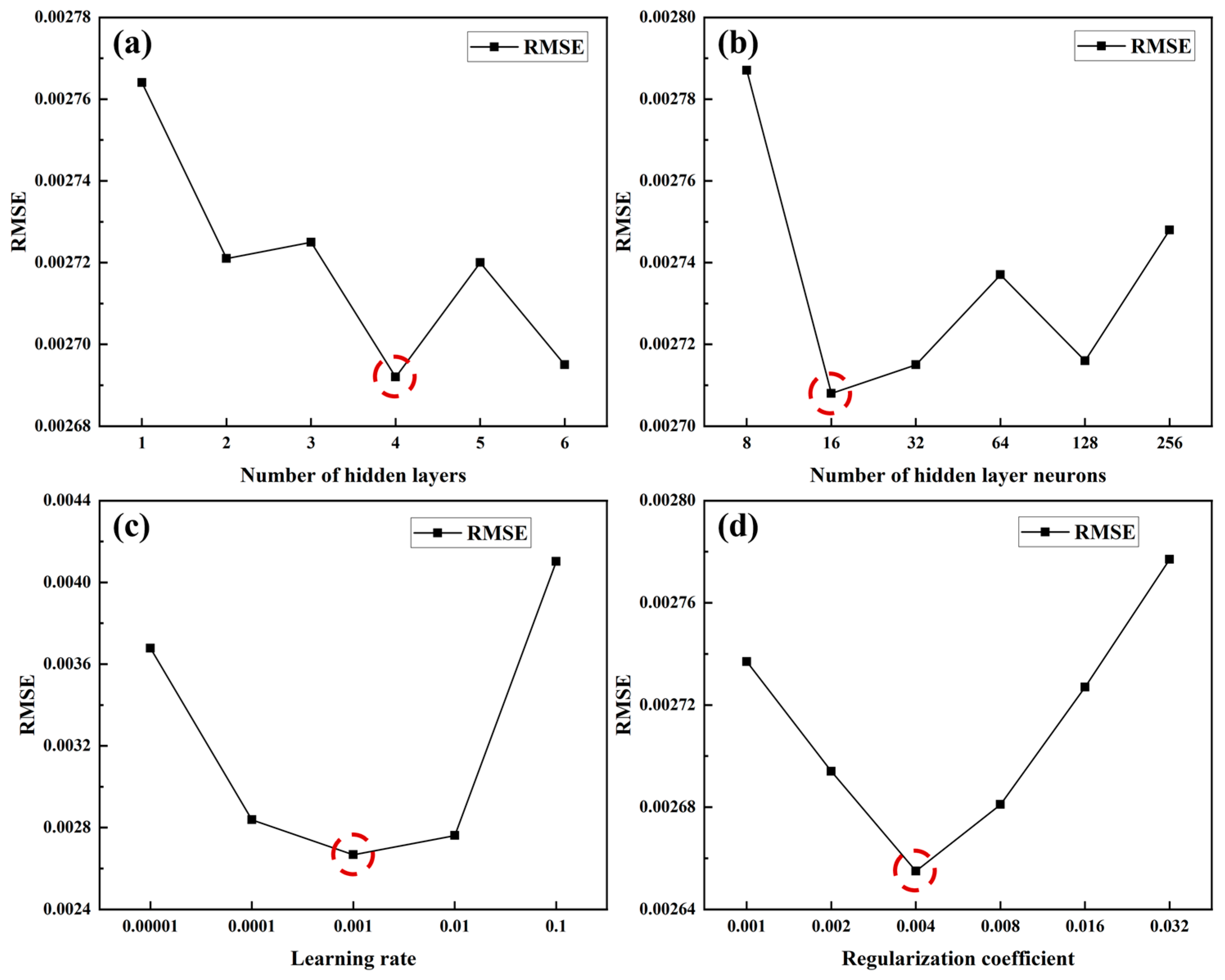
In this study, a grid-search procedure was adopted to determine the optimal ANN architecture and regularisation settings. The candidate hyperparameters included the number of hidden layers, the number of neurons in each hidden layer, the learning rate and the L² regularisation coefficient. For each combination in the predefined grid, the ANN was trained on the training folds and evaluated on the corresponding validation folds, and the average validation performance (in terms of R² and RMSE for endpoint sulphur) was used as the selection criterion. The influence of the main hyperparameters on model performance is summarised in Figure 13. Based on this analysis, the final ANN configuration was chosen as four hidden layers with 16 neurons in each layer, a learning rate of 0.001 and a regularisation coefficient of 0.004.

3.3.2. Optimal Model Interpretability Analysis

As is well known, NN models are composed of multiple layers, with each layer processing inputs through nonlinear activation functions. This hierarchical structure results in numerous complex transformations as data passes through the network. The output of each layer depends not only on the weights and biases of the previous layer but also on the nonlinear activation function applied, making NN “black-box” models. There is no clear, top-down relationship between the input and output, which necessitates the use of an interpretability tool such as SHAP value to visualize and analyze the model’s input-output relationships.

SHAP is a model interpretation method based on game theory [29]. SHAP quantifies the contribution of each feature to a model’s prediction. For complex models such as NN, SHAP provides both global and local explanations, helping us understand how features influence the prediction results. The core of SHAP is based on the Shapley value, a fair distribution method used in game theory to allocate cooperative gains. In the context of model interpretation, the model’s prediction can be viewed as the “reward,” and the features as the “players.” SHAP measures the contribution of each feature to the final prediction outcome.

For a given input sample $x$, the model’s prediction $f\left(x\right)$ can be expressed as the sum of individual feature contributions, as formulated in Equation (11):

$$f\left(x\right)={\mathrm{\varnothing }}_0+\sum _{i=1}^M{\mathrm{\varnothing }}_i$$

(11)

Here, ${\mathrm{\varnothing }}_0$ is the baseline value (typically the average predicted value in the training set) and ${\mathrm{\varnothing }}_i$ is the SHAP value for feature $i$ for this sample, which represents the contribution of that feature to the model’s prediction relative to the baseline.

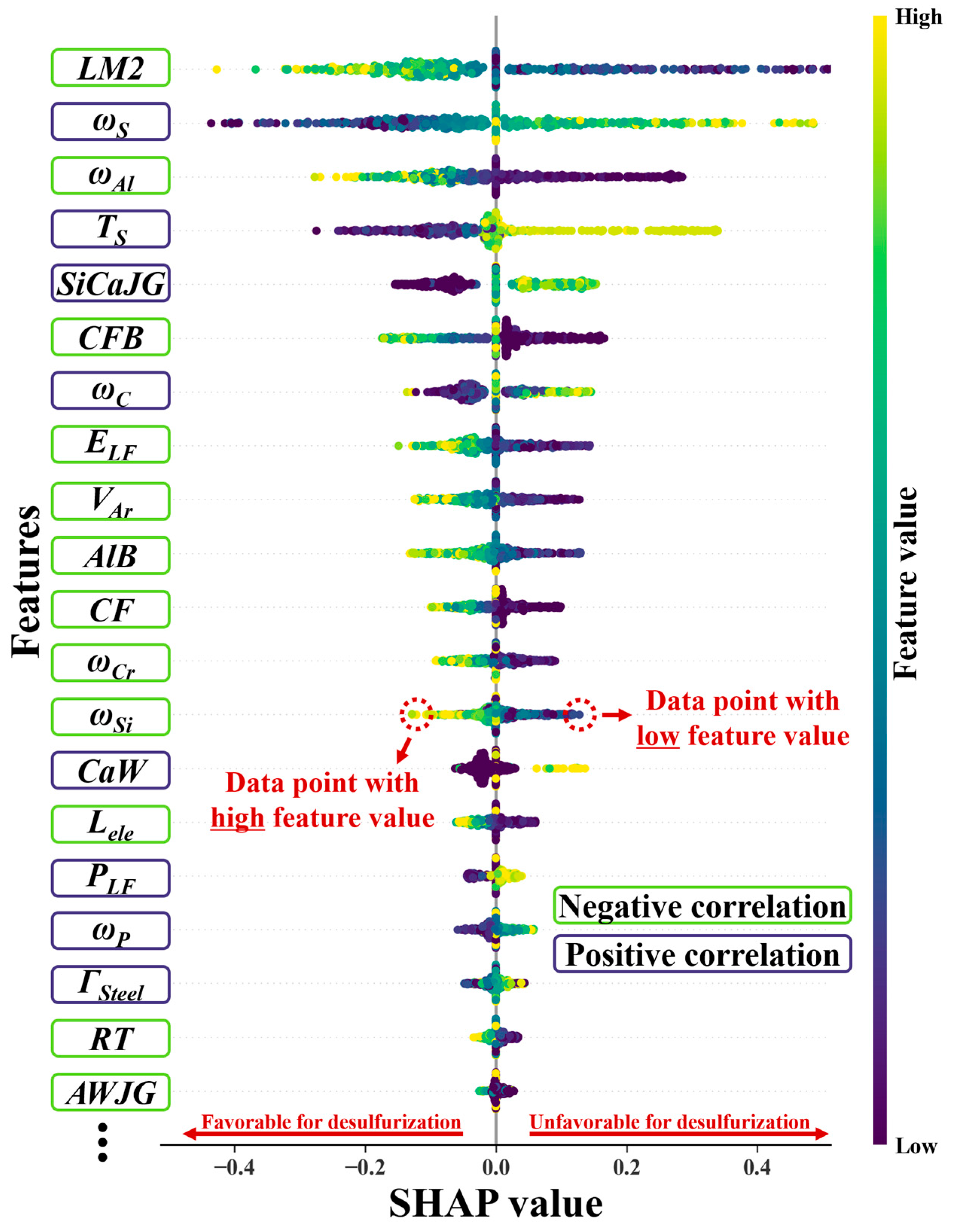
The interpretability analysis of the optimal model, the ANN, was conducted using the SHAP framework. SHAP values quantify the marginal contribution of each feature to the model output, thereby providing an interpretable link between the input variables and the predicted sulfur content. The resulting SHAP value distribution for the ANN model is illustrated in Figure 14, which visualizes the relative importance and influence direction of each feature on the desulfurization prediction results.

The plot for each feature is composed of scatter points derived from the SHAP values of all sample data. The scatter points on the left side of the vertical axis have a reducing effect on the dependent variable, while those on the right side increase the dependent variable. The color of the scatter points represents their values in the dataset, with points close to the purple color at the bottom of the color bar indicating smaller values and those close to yellow at the top indicating larger values. The features are ranked from top to bottom based on their impact on the LF end-point sulfur content. From the SHAP plot, it can be observed that higher values of LM2, ${\omega }_{\mathrm{A}\mathrm{l}}$, Lele, ELF, etc., are beneficial for desulfurization, showing a negative correlation with the LF end-point sulfur content. Higher values of ${\omega }_{\mathrm{C}}$, ${\omega }_{\mathrm{S}}$, SiCaJG, TS, etc., are unfavorable for desulfurization, showing a positive correlation with the LF end-point sulfur content. The remaining features have a smaller impact according to their SHAP values, which are not analyzed here.

Subsequently, this study validates the conclusions derived from the SHAP plot through metallurgical expert knowledge analysis:

Feeding Data Impact Analysis: Lime is used to combine with sulfur in the steel to form calcium sulfide, which is then removed through slagging in the LF reaction system. Therefore, high values of secondary lime LM2 are beneficial for desulfurization, with the data points located on the left side of the vertical axis. LM1, the primary lime, does not appear in the SHAP plot because it is a temporary substitute for LM2, used only when LM2 is not added. This condition is reflected in the dataset, where only 14 out of 5169 furnaces used LM1, making its data weight small and having almost no impact on the final sulfur content prediction. Sintered fluorspar CFB is used in the LF process as a slagging agent to lower the steel slag’s melting point, enhance slag fluidity, and facilitate the exchange of components between steel slag and molten steel, promoting sulfur removal. Therefore, high values of CFB are beneficial for desulfurization and are located on the left side of the vertical axis. The addition of SiCaJG is intended to remove aluminum oxides produced during the deoxidation process. Steel grades with higher initial sulfur content ${\omega }_{\mathrm{S}}$ produce more aluminum oxide during deoxidation, thus requiring more SiCaJG to remove these oxides. This condition is reflected in the SHAP plot, where SiCaJG shows a positive correlation with the LF end-point sulfur content.

Steel Element Impact Analysis: The initial sulfur content ${\omega }_{\mathrm{S}}$ directly influences the LF process’s end-point sulfur content, which is evident. Therefore, data points with high values of ${\omega }_{\mathrm{S}}$ are located on the right side of the vertical axis. The aluminum content ${\omega }_{\mathrm{A}\mathrm{l}}$ in the steel after the converter also affects the oxygen content in the steel due to the aluminum-oxygen balance. As ${\omega }_{\mathrm{A}\mathrm{l}}$ increases, the residual oxygen content in the steel decreases, which is a necessary condition for desulfurization. Therefore, data points with higher ${\omega }_{\mathrm{A}\mathrm{l}}$ values are located on the left side of the vertical axis. The positive correlation between the initial carbon content ${\omega }_{\mathrm{C}}$ and the LF end-point sulfur content occurs because steel grades with lower requirements for end-point sulfur also have lower carbon content, resulting in less removal of both elements.

Process Data Impact Analysis: The total electrical power input ELF in the LF process represents the total electrical power input, which is the driving force for the desulfurization reaction. Therefore, larger values of ELF improve the desulfurization effect, showing a negative correlation with the end-point sulfur content. Generally, higher temperatures during the LF phase lead to higher desulfurization efficiency; LF steel tapping temperature TS should be negatively correlated with the final sulfur content. However, steel grades with high sulfur content at the end of the converter process often also have high oxygen content. After deoxidation with aluminum wire in the LF process, the oxygen content still does not meet the standard and requires RH vacuum degassing treatment after the LF process. This requires a heating operation before LF tapping to prevent the molten steel temperature from being too low when entering the RH, which is reflected in the SHAP plot as a positive correlation between TS and the end-point sulfur content. Such misjudgment often occurs in data analysis work, highlighting the importance of integrating metallurgical expert knowledge into ML analysis. Expert knowledge serves as a bridge between real-world knowledge and data, establishing an efficient model with common-sense judgment ability.

4. Conclusions

This study developed a knowledge-guided, interpretable, machine learning framework for predicting endpoint sulphur content in LF refining based on industrial L2 data from high-purity iron and non-alloy steel production. A physically meaningful desulphurisation time window was defined from the simultaneous fulfilment of key refining conditions to the final argon-blowing stage, and multi-grade heats were grouped by K-means clustering to obtain representative operating modes. Within the selected cluster, four representative models—RF, XGBoost, SVM and ANN—were trained and evaluated using consistent train–test splitting and cross-validation schemes.

Among the candidate models, the ANN exhibited the best overall predictive performance for endpoint sulphur, achieving an R² of 0.7752, an RMSE of 0.0027 wt% and a MAE of 0.0017 wt% on the held-out industrial test set. Approximately 76.40% of heats showed an absolute prediction error within ±0.0025 wt% for sulphur, a tolerance band that is compatible with the sulphur specification used in the studied plant. These results indicate that the proposed framework can provide sufficiently accurate and robust predictions to serve as a practical decision-support tool for endpoint sulphur control in industrial LF operations.

Beyond prediction accuracy, SHAP combined with thermodynamic and transport considerations revealed that limestone addition, slag basicity, argon stirring conditions, refining time and initial sulphur content are the dominant variables governing sulphur removal. The observed SHAP trends are consistent with the expected influences of sulphide capacity, oxygen potential and steel–slag mass transfer, thereby enhancing the physical credibility of the model. The framework therefore not only delivers quantitative predictions but also offers metallurgically interpretable insight into how operating parameters should be adjusted to achieve specification-conforming sulphur levels while mitigating over-desulphurisation and reagent consumption.

It should be noted that the present validation is based on offline historical industrial data from a single plant and primarily focuses on one representative cluster of steel grades. Future work will extend the framework to additional clusters and steel grades, incorporate a more explicit representation of the temporal evolution of the desulphurisation process and conduct prospective online trials to quantify the impact of the model on process stability, reblow frequency and overall cost performance. Despite these limitations, the proposed knowledge-guided and interpretable modelling approach provides a promising foundation for intelligent endpoint sulphur control and can be generalised to related secondary refining operations.

References

1. Holappa, L.E.K.; Helle, A.S. Inclusion Control in High-Performance Steels. J. Mater. Process. Technol. 1995, 53, 177–186. [Google Scholar] [CrossRef]
2. Huang, D.; Huang, F. Coupled thermo-fluid stress analysis of Kambara Reactor with various anchors in the stirring of molten iron at extremely high temperatures. Appl. Therm. Eng. 2014, 73, 222–228. [Google Scholar] [CrossRef]
3. Schrama, F.N.H.; Beunder, E.M.; Van den Berg, B.; Yang, Y.; Boom, R. Sulphur removal in ironmaking and oxygen steelmaking. Ironmak. Steelmak. 2017, 44, 333–343. [Google Scholar] [CrossRef]
4. Lv, W.; Xie, Z.; Mao, Z.; Yuan, P.; Jia, M. Hybrid modelling for real-time prediction of the sulphur content during ladle furnace steel refining with embedding prior knowledge. Neural Comput. Appl. 2014, 25, 1125–1136. [Google Scholar] [CrossRef]
5. Xu, D.; Zhang, Q.; Huo, X.; Wang, Y.; Yang, M. Advances in data-assisted high-throughput computations for material design. Mater. Genome Eng. Adv. 2023, 1, e11. [Google Scholar] [CrossRef]
6. Pan, G.; Wang, F.; Shuang, C.; Wu, H.; Wu, G.; Gao, J.; Wang, S.; Gao, Z.; Zhou, X.; Mao, X. Advances in machine learning- and artificial intelligence-assisted material design of steels. Int. J. Miner. Metall. Mater. 2023, 30, 1003–1024. [Google Scholar] [CrossRef]
7. Zhang, R.; Yang, J. State of the art in applications of machine learning in steelmaking process modeling. Int. J. Miner. Metall. Mater. 2023, 11, 2055–2075. [Google Scholar] [CrossRef]
8. Ghalati, M.K.; Zhang, J.; El Fallah, G.M.A.M.; Nenchev, B.; Dong, H. Toward learning steelmaking—A review on machine learning for basic oxygen furnace process. Mater. Genome Eng. Adv. 2023, 1, e6. [Google Scholar] [CrossRef]
9. Tomažič, S.; Andonovski, G.; Škrjanc, I.; Logar, V. Data-Driven Modelling and Optimization of Energy Consumption in EAF. Metals 2022, 12, 816. [Google Scholar] [CrossRef]
10. Carlsson, L.S.; Samuelsson, P.B.; Jönsson, P.G. Interpretable Machine Learning-Tools to Interpret the Predictions of a Machine Learning Model Predicting the Electrical Energy Consumption of an Electric Arc Furnace. Steel Res. Int. 2020, 91, 2000053. [Google Scholar] [CrossRef]
11. Reimann, A.; Hay, T.; Echterhof, T.; Kirschen, M.; Pfeifer, H. Application and Evaluation of Mathematical Models for Prediction of the Electric Energy Demand Using Plant Data of Five Industrial-Size EAFs. Metals 2021, 11, 1348. [Google Scholar] [CrossRef]
12. Manojlović, V.; Kamberović, Ž.; Korać, M.; Dotlić, M. Machine learning analysis of electric arc furnace process for the evaluation of energy efficiency parameters. Appl. Energy 2022, 307, 118209. [Google Scholar] [CrossRef]
13. Sismanis, P. Prediction of Productivity and Energy Consumption in a Consteel Furnace Using Data-Science Models. Bus. Inf. Syst. 2019, 353, 85–99. [Google Scholar] [CrossRef]
14. Han, M.; Cao, Z. An improved case-based reasoning method and its application in endpoint prediction of basic oxygen furnace. Neurocomputing 2015, 149, 1245–1252. [Google Scholar] [CrossRef]
15. Zhou, M.; Zhao, Q.; Chen, Y. Endpoint prediction of BOF by flame spectrum and furnace mouth image based on fuzzy support vector machine. Optik 2019, 178, 575–581. [Google Scholar] [CrossRef]
16. Jo, H.; Hwang, H.J.; Phan, D.; Lee, Y.; Jang, H. Endpoint Temperature Prediction model for LD Converters Using Machine-Learning Techniques. In 2019 IEEE 6th International Conference on Industrial Engineering and Applications (ICIEA); IEEE: Piscataway, NJ, USA, 2019; pp. 22–26. [Google Scholar] [CrossRef]
17. Wang, X.; Han, M.; Wang, J. Applying input variables selection technique on input weighted support vector machine modeling for BOF endpoint prediction. Eng. Appl. Artif. Intell. 2010, 23, 1012–1018. [Google Scholar] [CrossRef]
18. Zhang, R.; Yang, J.; Wu, S.; Sun, H.; Yang, W. Comparison of the Prediction of BOF End-Point Phosphorus Content Among Machine Learning Models and Metallurgical Mechanism Model. Steel Res. Int. 2023, 94, 2200682. [Google Scholar] [CrossRef]
19. Wang, H.; Xu, A.; Ai, L.; Tian, N.; Du, X. An Integrated CBR Model for Predicting Endpoint Temperature of Molten Steel in AOD. ISIJ Int. 2012, 52, 80–86. [Google Scholar] [CrossRef]
20. Guan, C.; You, W.; Lin, X. Prediction Model ofEnd-point for AOD Furnace Based on Neural Network. In 2009 IEEE International Conference On Mechatronics and Automation; IEEE: Piscataway, NJ, USA, 2009; pp. 2426–2430. [Google Scholar] [CrossRef]
21. He, F.; Xu, A.; Wang, H.; He, D.; Tian, N. End Temperature Prediction of Molten Steel in LF Based on CBR. Steel Res. Int. 2012, 83, 1079–1086. [Google Scholar] [CrossRef]
22. Tian, H.; Liu, Y.; Li, K.; Yang, R.; Meng, B. A New AdaBoost.IR Soft Sensor Method for Robust Operation Optimization of Ladle Furnace Refining. ISIJ Int. 2017, 57, 841–850. [Google Scholar] [CrossRef]
23. Yang, Q.; Zhang, J.; Yi, Z. Predicting molten steel endpoint temperature using a feature-weighted model optimized by mutual learning cuckoo search. Appl. Soft Comput. 2019, 83, 105675. [Google Scholar] [CrossRef]
24. Xin, Z.; Zhang, J.; Zheng, J.; Jin, Y.; Liu, Q. A Hybrid Modeling Method Based on Expert Control and Deep Neural Network for Temperature Prediction of Molten Steel in LF. ISIJ Int. 2022, 62, 2021–2251. [Google Scholar] [CrossRef]
25. Kargul, T.; Falkus, J. A Hybrid Model of Steel Refining in The Ladle Furnace. Steel Res. Int. 2010, 81, 953–958. [Google Scholar] [CrossRef]
26. Xin, Z.; Zhang, J.; Jin, Y.; Zheng, J.; Liu, Q. Predicting the alloying element yield in a ladle furnace using principal component analysis and deep neural network. Int. J. Miner. Metall. Mater. 2023, 30, 335–344. [Google Scholar] [CrossRef]
27. Laha, D.; Ren, Y.; Suganthan, P.N. Modeling of steelmaking process with effective machine learning techniques. Expert Syst. Appl. 2015, 42, 4687–4696. [Google Scholar] [CrossRef]
28. Yang, J.; Zhang, J.; Guo, W.; Gao, S.; Liu, Q. End-point Temperature Preset of Molten Steel in the Final Refining Unit Based on an Integration of Deep Neural Network and Multi-process Operation Simulation. ISIJ Int. 2021, 61, 2020–2540. [Google Scholar] [CrossRef]
29. Lundberg, S.M.; Lee, S. A Unified Approach to Interpreting Model Predictions. In 31St Conference On Neural Information Processing Systems; Curran Associates Inc.: Red Hook, NY, USA, 2017; pp. 4768–4777. [Google Scholar] [CrossRef]
Figure 1. ML application process in production.
Processes 14 01118 g001
Figure 2. Time series data sampling process based on expert knowledge.
Processes 14 01118 g002
Figure 3. Distribution histograms of LF element contents, feedings, and process data.
Processes 14 01118 g003
Figure 4. Schematic diagram of K-Means clustering algorithm, using the elbow method to determine the number of clusters. The colors on the colorbar represent the Euclidean distance of the points from the cluster centers.
Processes 14 01118 g004
Figure 5. Optimized clustering result for k = 3.
Processes 14 01118 g005
Figure 6. Dimensionality reduction method based on feature correlation heatmap using Pearson correlation coefficient.
Processes 14 01118 g006
Figure 7. The prediction results of the test set of the RF model.
Processes 14 01118 g007
Figure 8. The prediction results of the test set of the XGBoost model.
Processes 14 01118 g008
Figure 9. The prediction results of the test set of the SVM model.
Processes 14 01118 g009
Figure 10. The prediction results of the test set of the ANN model.
Processes 14 01118 g010
Figure 11. Training and validation loss curves of the ANN model as a function of epoch.
Processes 14 01118 g011
Figure 12. (a) RF training performance; (b) XGBoost training performance; (c) SVM training performance; (d) ANN training performance.
Processes 14 01118 g012
Figure 13. Influence of key ANN hyperparameters on model performance (RMSE): (a) number of hidden layers; (b) number of neurons per hidden layer; (c) learning rate; (d) regularization coefficient.
Processes 14 01118 g013
Figure 14. Summary plot of SHAP values based on the tuned ANN model.
Processes 14 01118 g014