Generalized Vision-Based Coordinate Extraction Framework for EDA Layout Reports and PCB Optical Positioning

Abstract

Automated optical inspection (AOI) technologies are widely used in PCB and semiconductor manufacturing to improve accuracy and reduce human error during quality inspection. While existing AOI systems can perform defect detection, they often rely on pre-defined camera positions and lack flexibility for interactive inspection, especially when the operator needs to visually verify solder pad conditions or examine specific layout regions. This study focuses on the front-end optical positioning and inspection stage of the AOI workflow, providing an automated mechanism to link digitally generated layout reports from EDA layout tools with real PCB inspection tasks. The proposed system operates on component-placement reports exported by EDA layout environments and uses them to automatically guide the camera to the corresponding PCB coordinates. Since PCB design reports may vary in format and structure across EDA tools, this study proposes a vision-based extraction approach that employs Hough transform-based region detection and a CNN-based digit recognizer to recover component coordinates from visually rendered design data. A dual-axis sliding platform is driven through a hierarchical control architecture, where coarse positioning is performed via TB6600 stepper control and Bluetooth-based communication, while fine alignment is achieved through a non-contact, gesture-based interface designed for clean-room operation. A high-resolution autofocus camera subsequently displays the magnified solder pads on a large screen for operator verification. Experimental results show that the proposed platform provides accurate, repeatable, and intuitive optical positioning, improving inspection efficiency while maintaining operator ergonomics and system modularity. Rather than replacing defect-classification AOI systems, this work complements them by serving as a positioning-assisted inspection module for interactive and semi-automated PCB quality evaluation.

1. Introduction

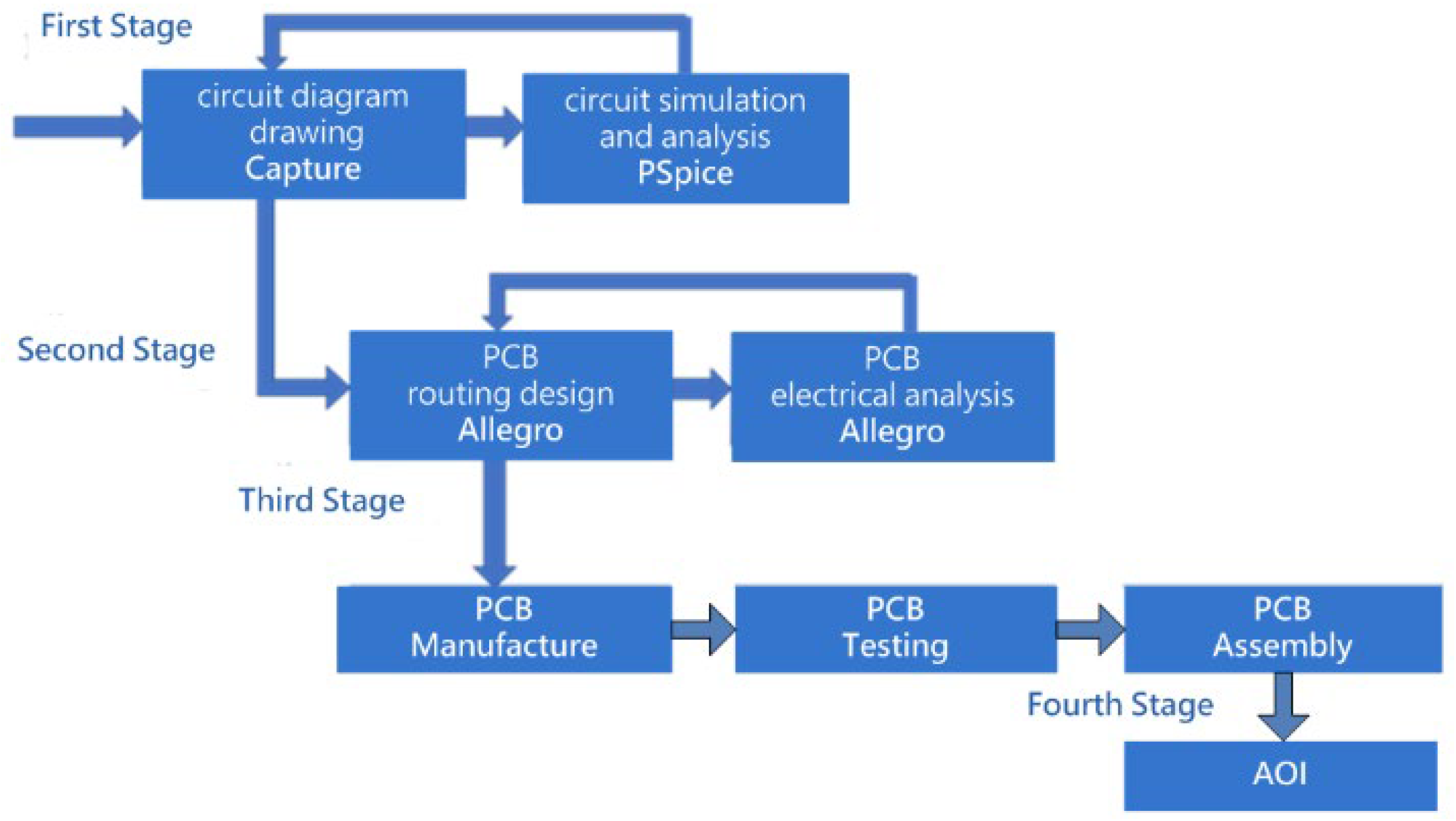
Modern PCB design environments typically allow engineers to export a placed component report (PCR), a type of layout report that records the coordinate positions of each device on the board. Depending on the EDA tool and version, these reports may be provided in HTML, CSV, or rasterized table formats, and their structural consistency can vary considerably. Such variability makes it difficult to reliably retrieve coordinate data through direct text parsing or conventional web-scraping techniques, motivating the need for a vision-based and format-independent extraction approach. In this study, a vision-based text extraction approach is adopted to overcome this limitation, enabling automatic retrieval of component coordinates for subsequent optical positioning and inspection. This study extends the PCB inspection workflow by integrating an optical positioning and inspection platform capable of automatically interpreting PCR data exported from PCB layout tools and guiding the camera to the corresponding physical PCB location for visual inspection. The traditional PCB manufacturing workflow typically concludes once layout, fabrication, and assembly are completed, shown in Figure 1. However, in practical production environments, localized visual inspection of solder joints remains necessary to ensure quality. As PCBs continue to evolve toward higher density and miniaturized components, accurate optical positioning becomes more critical, particularly when engineers must verify solder coverage or component alignment at specific board regions. Conventional AOI systems primarily focus on automated defect detection and often lack flexible mechanisms for operator-guided verification or interactive inspection. Therefore, a positioning-assisted inspection mechanism is still required in many production scenarios to support human-in-the-loop visual confirmation.

The proposed system automatically extracts component coordinates from PCR layout reports exported by PCB design tools and maps them to a two-stage movement platform consisting of coarse positioning and gesture-assisted fine alignment. A high-resolution camera then displays the magnified solder region on a monitor, enabling operators to verify solder quality or placement accuracy without physically manipulating the device. While tools such as Allegro may offer HTML-based reports that allow partial direct parsing, structural inconsistency across different PCB layout tools and file versions prevents reliable extraction. Therefore, the proposed CNN-assisted visual parsing pipeline is designed to remain compatible with non-semantic or image-based outputs, including rasterized tables, screenshots, and PDF exports. To recover coordinate values from layout reports exported by PCB design tools, a Hough Transform-based segmentation method is employed to reconstruct the grid structure of the PCR table, after which digit isolation and recognition are performed. This process enables precise translation from digitally reported layout data to their corresponding physical positions on the PCB.

Additionally, a non-contact gesture interface is adopted to support fine alignment, which is particularly suitable for clean-room or sensitive manufacturing environments where physical joysticks are less desirable. Accordingly, the proposed platform does not replace full AOI systems but instead complements them as a front-end optical positioning module that bridges digitally extracted placement data with interactive human verification on the physical PCB.

2. Related Work

2.1. Coordinate Extraction from Rasterized PCRs

Industrial EDA tools generally export design reports in either semantic (text-based) or image-based formats. Text-based outputs can be directly parsed through scripting or HTML/CSV-based processors, whereas image-based reports visually embed tabular content without structural metadata, making conventional parsers ineffective for extracting numerical values. Although a Placed Component Report (PCR) can be exported as a semantic HTML table in certain PCB layout tools (e.g., Allegro), its structure may vary depending on software version and configuration. To ensure robust and consistent data retrieval across different report types, this study adopts a vision-based approach to extract component coordinates.

Prior studies on image-based table reconstruction have shown that when tabular layout is rasterized rather than semantically encoded, coordinate values cannot be retrieved through HTML parsing and must instead be reconstructed through vision-based processing [1,2,3,4]. These studies indicate that segmentation and digit recognition are required once the tabular layout is visually encoded. Following this approach, the present work treats PCR layout reports as rasterized engineering tables and reconstructs its coordinate fields through visual layout detection and digit extraction to enable automated positioning on the physical PCB.

2.2. Raster Table Reconstruction Using Hough Transform

Raster-form engineering documents often lose explicit row and column boundaries due to aliasing or canvas-based rendering. In such cases, table structures cannot be reliably recovered using conventional histogram projection. The Hough Transform, originally proposed for line detection [5] and later extended for improved robustness by Duda and Hart [6], is better suited for reconstructing structural grid lines in degraded or non-semantic tabular data. Variants such as the Randomized and Gradient Hough Transform [7,8] further enhance detection stability in low-contrast industrial imagery, which aligns with the characteristics of rasterized and weakly structured placement reports commonly generated by PCB layout tools. Prior works have also demonstrated its effectiveness in extracting structural geometry from partially discontinuous edges in engineering documents [9,10].

However, when multiple digits are densely packed within a single grid cell, histogram-based segmentation becomes unreliable because vertical or horizontal projections produce overlapping peaks and valleys. To address this, the proposed method first employs Hough Transform-based grid reconstruction to determine the bounding regions of each cell, followed by a pixel-scanning approach that sequentially isolates individual digits for recognition. This two-stage process effectively overcomes the limitations of projection methods in dense numeric layouts and enables precise coordinate extraction from rasterized PCRs.

2.3. Digit Segmentation Methods

Digit segmentation is a fundamental step in extracting structured numerical information from images and has been widely adopted in applications such as license plate recognition, invoice analysis, and industrial document parsing. Early projection-based segmentation methods separated adjacent digits by detecting valleys in horizontal or vertical histograms, offering computational simplicity but struggling when characters were closely spaced or connected. Akhtar et al. [11] adopted this approach in their license plate recognition framework, achieving 90.9% accuracy through a four-stage process consisting of preprocessing, plate localization, digit segmentation, and recognition using a random forest classifier. To overcome the over-segmentation problem caused by irregular spacing or connected handwritten characters, Rajput et al. [12] proposed an adaptive vertical pixel-counting algorithm that dynamically adjusted segmentation thresholds according to local pixel density. Building upon these efforts, Zin et al. [13] combined labeling and projection techniques to enhance segmentation robustness for printed documents, while Ren et al. [14] incorporated width–spacing ratio features to suppress noise and border interference in license plate characters. These studies demonstrate that projection-based segmentation remains efficient for well-spaced digits but becomes less effective for densely packed or irregularly aligned numeric data.

Since PCR layout reports render coordinate fields as rasterized images without explicit cell boundaries, traditional projection-based methods are insufficient for reliable digit isolation. Therefore, this study employs a pixel-scanning approach after Hough Transform-based grid reconstruction to sequentially extract individual digits within each identified cell, enabling accurate coordinate reconstruction for downstream CNN-based recognition.

2.4. CNN-Based Neural Networks

Early neural network research identified the limitations of single-layer perceptrons in handling nonlinear classification tasks [15], which led to the development of multilayer perceptrons (MLPs) and the backpropagation algorithm [16,17]. These advances laid the foundation for modern deep learning architectures. Subsequent work by LeCun demonstrated the effectiveness of convolutional neural networks (CNNs) for handwritten digit recognition [18], culminating in the LeNet-5 framework [19], which has been widely adopted in practical document understanding tasks [20]. Additionally, with NVIDIA’s introduction of the Compute Unified Device Architecture (CUDA), general-purpose computing on Graphics Processing Units (GPUs) became feasible, allowing neural networks to perform large-scale parallel computations. The CUDA significantly accelerated the training of deep learning models, fostering the rapid advancement of CNN-based neural networks, including LeNet [21], AlexNet [22], VGGNet [23], and ResNet [24].

With the rise of deep learning, CNN-based models have become the mainstream approach for digit recognition across numerous applications, including postal code reading, bank check processing, and industrial document parsing [25,26,27,28,29,30], illustrating their robustness in extracting structured numeric information from images. To facilitate large-scale benchmarking and accelerate research in real-time recognition, LeCun and collaborators released the MNIST dataset [31], consisting of 60,000 training and 10,000 testing samples of 28 × 28 grayscale digit images with corresponding labels. In this study, a lightweight CNN is similarly employed to recognize segmented coordinate digits extracted from rasterized PCRs, enabling reliable numeric reconstruction for downstream positioning.

2.5. Gesture Recognition for Non-Contact Control

Gesture-based interaction has been widely adopted in recent years for hands-free control in industrial and assistive applications, providing an effective alternative to conventional physical interfaces. MediaPipe (version 0.10.x, Google LLC, Mountain View, CA, USA), a lightweight cross-platform framework, enables real-time hand landmark detection and has been extensively applied in various recognition systems. For instance, Medina et al. [32] integrated the MediaPipe Holistic detection model with Long Short-Term Memory (LSTM) and Multilayer Perceptron (MLP) architectures to achieve real-time gesture recognition. In Caporusso et al. [33], an automatic face mask detection method was implemented using the MediaPipe framework, while Bao et al. [34] employed MediaPipe-based hand tracking combined with an LSTM classifier to recognize nine distinct gestures. Hsieh et al. [35] proposed an air-writing recognition method based on deep CNNs, which captures handwriting trajectories without virtual delimiters to enhance usability, whereas Alam et al. [36] developed a 3D trajectory-based air-writing system using a depth camera and trajectory normalization. In this study, a hand detection algorithm was employed to extract 21 hand landmark coordinates using the MediaPipe framework for gesture recognition. These coordinates were then mapped to control commands for the fine positioning stage of the inspection platform. In the context of PCB inspection, non-contact control is particularly advantageous because physical joysticks or buttons are less suitable in clean-room or high-precision assembly environments. Accordingly, the proposed gesture-based mechanism complements the coarse movement of the XY platform, allowing operators to intuitively adjust the camera position without direct hardware contact.

3. Hardware Architecture

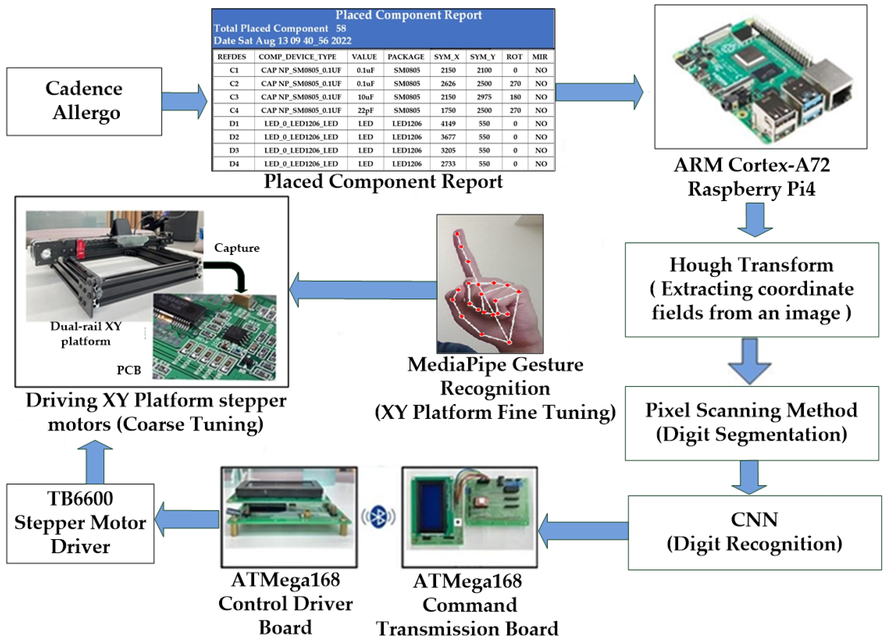
This research develops an optical inspection system based on an XY platform, capable of automatically interpreting the component placement reports generated by the PCB layout software (OrCAD PCB Editor, version 17.2, Cadence Design Systems, San Jose, CA, USA), and serving as a positioning-assisted inspection module for human-in-the-loop visual verification for solder joint inspection. Through a two-stage adjustment process comprising coarse and fine tuning, the XY platform moves the camera to the designated component coordinates on the PCB, enabling operators to visually inspect the solder paste quality of SMD solder joints on a large screen. In this dual-stage positioning mechanism, coarse positioning drives the camera toward the approximate component location, while gesture-based fine alignment provides precise incremental adjustment for accurate visual verification. The overall system architecture is illustrated in Figure 2.

First, the ARM Cortex-A72-based Raspberry Pi 4 microprocessor (Raspberry Pi Foundation, Cambridge, UK) reads the Placed Component Report (PCR) exported from the PCB layout tool. After the coordinate table regions are extracted using the Hough transform, digit segmentation is performed using a pixel scanning method, and the segmented digits are subsequently recognized by a CNN to identify the coordinate positions of PCB components. The extracted data are then transmitted wirelessly via Bluetooth to the ATmega168-based driver control board (Microchip Technology Inc., Chandler, AZ, USA). Using a TB6600 stepper motor driver (Toshiba Corporation, Tokyo, Japan), the dual-axis sliding rail XY platform moves to the designated area, completing the coarse positioning stage. The camera subsequently captures the PCB region and project it onto the large display of the AOI interface. Finally, MediaPipe is employed to extract 21 hand landmark coordinates and analyze gesture trajectories, which are then converted into fine adjustment commands for the stepper motors, thereby achieving precise and contact-free optical inspection.

3.1. Embedded Microprocessor

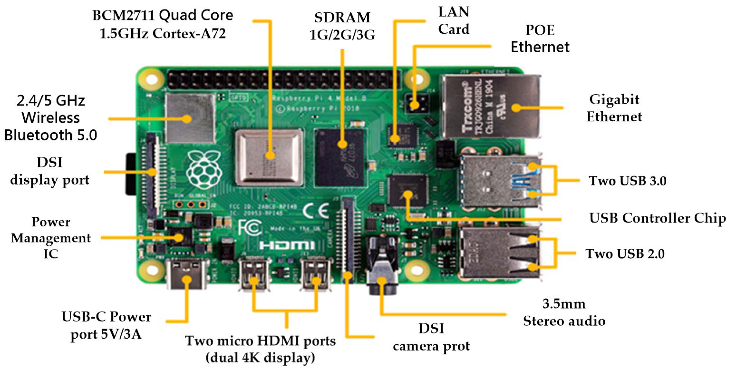
The system is implemented on a Raspberry Pi 4, which serves as the main embedded controller responsible for parsing the Placed Component Report (PCR), reconstructing the rasterized table structure, and performing CNN-based digit recognition. The Raspberry Pi was selected due to its integrated Linux environment, built-in wireless connectivity, and sufficient computational capability to handle both image-based coordinate extraction and gesture-based fine positioning. Once the component coordinates are decoded, they are transmitted wirelessly to the motion control module to drive the XY platform. The hardware configuration of the embedded controller is shown in Figure 3.

It should be clarified that the CNN used for digit recognition is trained offline on a workstation, and only the final inference model is deployed on the Raspberry Pi. This significantly reduces computational requirements during the coarse positioning stage. During fine adjustment, MediaPipe performs real-time hand landmark extraction and therefore imposes a higher processing load. In this work, a Raspberry Pi 4 provides acceptable performance after pipeline optimization, as the computationally intensive CNN training is performed offline and only lightweight inference is executed during runtime. However, for lower latency and smoother gesture responsiveness, a Raspberry Pi 5 or equivalent ARM-based embedded platform is recommended.

3.2. Embedded Microcontroller

Two ATmega168 microcontrollers (Toshiba Corporation, Tokyo, Japan) are employed in the proposed system to implement a modular and hierarchical control architecture, as illustrated in Figure 2. The first unit functions as the command-transmission controller, receiving decoded coordinates from the host platform via UART and relaying them wirelessly over Bluetooth, while the second unit executes timing-critical stepper motor control for XY motion. This separation allows the motion-control module to operate independently of the host hardware, enabling the system to remain compatible not only with Raspberry Pi but also with PCs or other embedded platforms that may not include native Bluetooth support. In this way, the dual-microcontroller design preserves cross-platform portability and ensures that the motion layer remains interchangeable even if the upstream computing environment is replaced.

3.3. Stepper Motor Driver Module

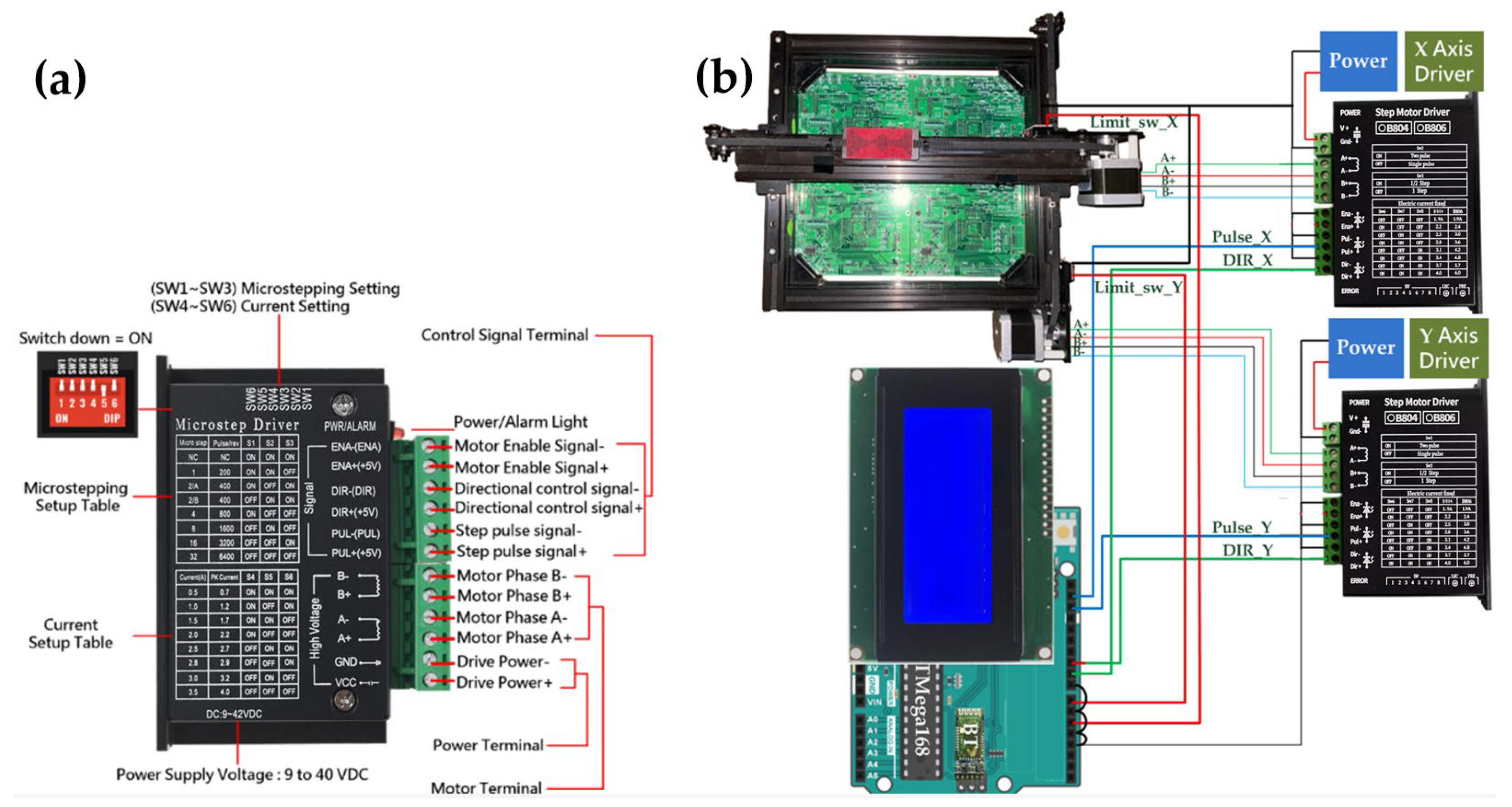
The stepper motor driver module used in this system is the TB6600 (Figure 4), which provides the required current amplification and microstepping control for stable XY motion. The driver receives pulse and direction signals from the ATmega168 motion-control board and converts them into precise mechanical displacement along the X and Y axes. Microstepping enhances positioning smoothness and minimizes vibration during coarse alignment. The wiring configuration adopts a standard pulse/dir interface, allowing the motion driver to remain interchangeable regardless of the upstream controller. Figure 4a is retained to illustrate the control-signal interface layout rather than electrical specifications, as these terminals define how the microcontroller interfaces with the motion layer in the proposed architecture. The wiring connections among the TB6600 driver module, the dual-axis XY platform, and the ATmega168 motion-control board are illustrated in Figure 4b.

3.4. XY Platform with Mounted Camera

The XY positioning platform is constructed using orthogonally arranged linear guide rails to provide stable and repeatable motion along both axes, as shown in Figure 5a. The camera module is mounted directly on the X-axis sliding carriage (Figure 5b), enabling the optical assembly to move synchronously with the platform during coarse positioning. A linear-rail structure is adopted to minimize vibration and mechanical backlash, which is essential for maintaining image sharpness during solder-joint inspection. Motion commands generated by the GUI are transmitted via a Bluetooth communication interface to the XY platform control board, which interprets the commands independently of the underlying mechanical structure. Because the motion-control interface is implemented at the command level and decoupled from the mechanical configuration, the mechanical platform can be scaled or replaced without requiring modifications to the control architecture.

A sliding block is installed on the X-axis linear guide rail, allowing it to move reciprocally along the track. The sliding block is equipped with a camera module for image acquisition. The linear guide rail provides a total stroke range of 200 mm. To enhance mechanical rigidity, the rail is integrated with an aluminum extrusion frame, ensuring structural stability during motion. NEMA 17 stepper motors (generic industrial standard) are employed on both the X- and Y-axis guide rails. Each motor drives a GT2 timing belt through a synchronous pulley, converting rotational motion into linear translation of the sliding block. In the timing belt mechanism, one full revolution of the motor corresponds to 20 pulley teeth. Given the GT2 belt pitch of 2 mm per tooth, one motor revolution results in a 40 mm linear displacement of the belt, enabling the sliding block to travel 40 mm per revolution. The linear displacement per micro-step of the sliding block along the guide rail is given by

$$d_N={\displaystyle \frac{40 \mathrm{m}\mathrm{m}}{(2\times n\times Z_r)\times N}}$$

(1)

where $n$ represents the number of motor phases, $Z_r$ denotes the number of rotor teeth, and $N$ is the microstepping division ratio of the stepper motor. In this system, the NEMA 17 stepper motor is a two-phase ($n=2$), four-pole device with 50 rotor teeth ($Z_r=50$). The stepper motor driver module is configured to operate in a 1/4 microstepping mode ($N=4$) via the DIP switch settings. Substituting these parameters into Equation (1), the resulting linear displacement per micro-step is calculated to be 0.05 mm. It should be noted that the derived displacement of 0.05 mm per step represents a theoretical resolution based on the microstepping configuration. In practical operation, the effective positioning resolution may be affected by mechanical factors such as backlash, belt elasticity, and acceleration dynamics.

The STEP input of the TB6600 stepper motor driver is supplied by the ATmega168 microcontroller, which generates a 1 kHz square-wave pulse train with a 50% duty cycle. Since the driver counts a step on each rising edge of the STEP signal, the effective step rate is equal to the pulse frequency $f$. Combining this pulse rate with the micro-step displacement $d_N$ obtained from Equation (1), the translational speed of the XY stage can be expressed as

$$v_N=d_N\times f\times 0.1\left({\displaystyle \frac{\mathrm{c}\mathrm{m}}{\mathrm{s}}}\right)$$

(2)

where the factor 0.1 converts the displacement unit from millimeters to centimeters. With $d_N=0.05 \mathrm{m}\mathrm{m}/\mathrm{s}\mathrm{t}\mathrm{e}\mathrm{p}$ and $f=1000 \mathrm{s}\mathrm{t}\mathrm{e}\mathrm{p}\mathrm{s}/\mathrm{s}$, the nominal stage velocity is $v_N=5 \mathrm{c}\mathrm{m}/\mathrm{s}$, which ensures a sufficiently fast coarse positioning of the sliding block toward the target component location.

A limit switch is installed at the endpoint of each guide rail to define the maximum travel range. When the sliding block reaches the endpoint and triggers the limit switch, the system immediately commands the stepper motor to stop, preventing mechanical collision or damage. The limit switch also serves as a homing reference for the platform, ensuring that each motion cycle begins from a consistent reference position.

4. Digital Recognition Algorithm

4.1. Hough Transform

To successfully extract image segments of component placements from the PCR layout report, this study employs the Hough Transform to detect horizontal, vertical, and border lines in the image. By calculating the distance between adjacent horizontal lines and between adjacent vertical lines, the coordinates filed of each component can be control isolated. In practical applications, a Cartesian coordinate system is not suitable for representing image space. This is because certain special vertical lines in image space, such as $x=c$, have an infinite slope, making them impossible to represent in the parameter space. 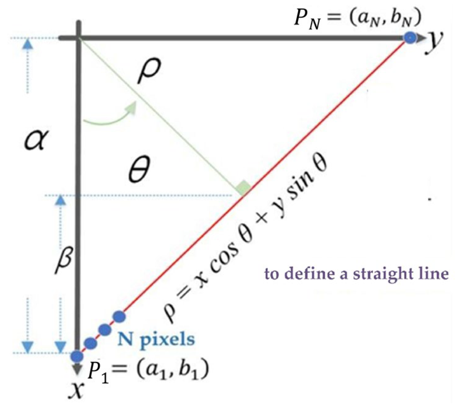Therefore, using polar coordinates $(\rho ,\theta )$ to formulate the Hough Transform problem is more appropriate, as it avoids the issue of infinite slope. In this study, the Hesse normal form is adopted to express the polar coordinate equation of a straight line, where $\rho$ represents the perpendicular distance from the origin O to the line, and $\theta$ denotes the angle between the x-axis and the perpendicular to the line (Figure 6). From the figure, the following relationship can be derived.

$$\rho =\alpha \mathrm{c}\mathrm{o}\mathrm{s}\theta =\left(x+\beta \right) \mathrm{c}\mathrm{o}\mathrm{s}\theta =\left(x+y \mathrm{t}\mathrm{a}\mathrm{n}\theta \right)\mathrm{c}\mathrm{o}\mathrm{s}\theta =x \mathrm{c}\mathrm{o}\mathrm{s}\theta +y \mathrm{s}\mathrm{i}\mathrm{n}\theta .$$

(3)

The traditional Hough Transform converts the image space into a parameter space and employs a voting algorithm to identify local maxima, thereby determining the perpendicular distance from each line in the image to the origin, as well as the angle it forms with the X-axis. The underlying principles of this transformation are detailed in [37].

Assuming there is a straight line in the image composed of $N$ pixel points, including two endpoints with pixel coordinates $P_1=(a_1,b_1)$, $P_N=(a_N,b_N)$, as illustrated in Figure 6, each of the $N$ pixel points from the image space can be substituted into (3) to obtain $N$ curve equations in the parameter space, as represented by (4).

$$L_n: \rho =a_n\mathrm{c}\mathrm{o}\mathrm{s}\theta +b_n\mathrm{s}\mathrm{i}\mathrm{n}\theta , n=1\dots N.$$

(4)

In the Hough Transform, the parameter space is defined by the polar coordinates ($\rho$, $\theta$), where $\theta$ denotes the angle of the line normal and ρ represents the perpendicular distance from the origin to the line. To construct the voting accumulator, the parameter space is discretized into a finite set of bins. In this work, the polar angle $\theta$ is discretized over the range [0°, 180°] with a resolution of 1°, resulting in $s$ = 180 discrete angular bins. For the radial parameter $\rho$, pixel-level precision is adopted. The range of $\rho$ is determined by the diagonal length of the image, and the number of radial bins $r$ is accordingly set to cover all possible perpendicular distances from the origin to a line in the image. Based on these discretization settings, a two-dimensional accumulator array $M\in R^{r\times s}$ is constructed and initialized with all elements set to zero. For each pixel point ($a_n$, $b_n$) belonging to an edge or line candidate in the image, the corresponding curve in the parameter space is computed using (4). Each discretized ($\rho$, $\theta$) pair lying on this curve increments the corresponding accumulator cell $M\left[\rho \left]\right[\theta \right]$ by one vote. After all $N$ pixel points have contributed their votes, accumulator cells that receive votes from a larger number of curves indicate stronger evidence of a line. The cell ($\rho$*, $\theta$*) with the maximum accumulated votes therefore corresponds to the most likely line parameters in the image.

For each pixel point $P_n=\left(a_n,b_n\right)$ in the image space, where $n=1\dots N$, substituting $\left(a_n,b_n\right)$ into (4) yields a sinusoidal curve $L_n$ in the parameter space. Given that $\theta$ is discretized into $s$ = 180 angular bins over $\theta \in [0°,179°]$, each curve contributes one vote to the accumulator for every discrete $\theta$ value. Let ${\theta }_m (m=0,\dots ,s-1)$ denote the m-th discretized angular bin of θ. Specifically, for a fixed pixel point $P_n$, $\theta$ is swept over all discrete bins ${\theta }_m$, and the corresponding $\rho$ values are computed as ${\rho }_m=a_{n}cos{\theta }_m+b_{n}sin{\theta }_m$. Each computed pair (${\rho }_m$, ${\theta }_m$) is mapped to the corresponding discretized accumulator index, and the voting array is updated by $M\left[{\rho }_m\left]\right[{\theta }_m\right]$ ← $M\left[{\rho }_m\left]\right[{\theta }_m\right]+1$. Therefore, each pixel point contributes $s$ votes in total, and processing $N$ pixel points results in $N\times s$ accumulator updates. After all votes are accumulated, peaks in $M$ indicate parameter pairs ($\rho$, $\theta$) that are consistent with many pixel points, i.e., a likely straight line in the image. In summary, the accumulator has a size of $r\times s$, and the voting procedure performs $N\times s$ updates in total. The most probable line parameters are obtained by locating the maximum value in the accumulator:

$$\left({\rho }^{*},{\theta }^{*}\right)=\arg \mathrm{m}\mathrm{a}\mathrm{x}\_\{\mathsf{\rho },\mathsf{\theta }\}\mathrm{M}(\mathsf{\rho },\mathsf{\theta }),\mathrm{w}\mathrm{h}\mathrm{e}\mathrm{r}\mathrm{e} \mathsf{\rho }\in [0,r-1],\mathsf{\theta }\in [0,s-1].$$

(5)

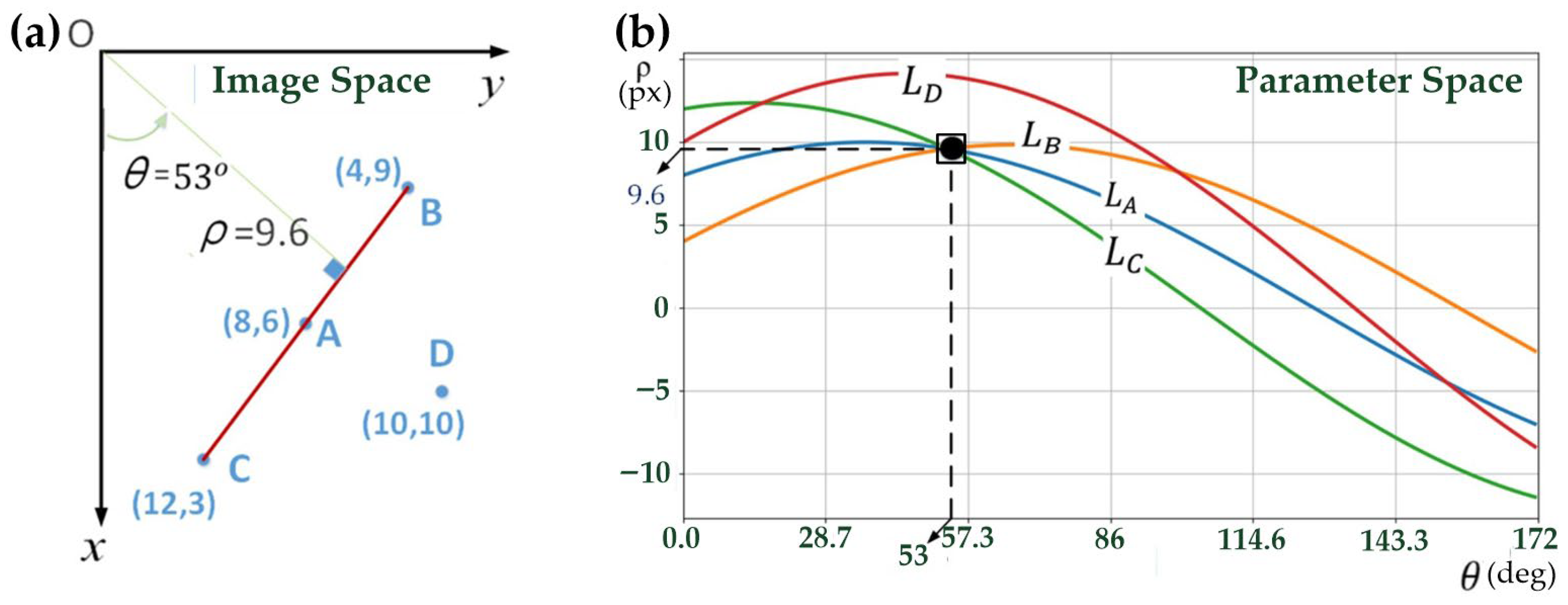
To illustrate how different entries in the accumulator array receive different numbers of votes, Figure 7 provides an intuitive example in both the image space and the parameter space. In the image space, four pixel points A, B, C, and D are considered, where points A, B, and C lie on the same straight line, while point D does not. When these points are transformed into the parameter space using the Hough Transform, each pixel point generates a corresponding sinusoidal curve (denoted as $L_A,L_B,L_C,$ and $L_D$). Because points A, B, and C are collinear, their corresponding curves intersect at a common point $\left({\rho }^{*},{\theta }^{*}\right)=(9.6,{53}^{°})$, which represents the parameters of the underlying straight line. In contrast, the curve generated by point D does not pass through this intersection. As a result, the accumulator cell corresponding to $\left({\rho }^{*},{\theta }^{*}\right)=(9.6,{53}^{°})$ receives multiple votes (one from each collinear pixel), whereas other cells receive fewer votes. This voting mechanism naturally leads to different occurrence counts in the accumulator array, and the cell with the maximum vote count indicates the most probable line in the image. Note that although $\rho$ may take negative values in the continuous parameter space for illustrative purposes, in practical implementation the accumulator is constructed using non-negative $\rho$ values, with the maximum range determined by the image diagonal length.

Unlike conventional engineering tables, the PCR layout reports often adopts a highly compact raster layout, where minimal row height and column width cause histogram-based peak detection to become ambiguous. In addition, raster aliasing causes partial line breaks, further reducing projection reliability. For this reason, Hough-based detection is adopted, as it remains stable even when the geometric structure is visually degraded or discontinuous.

4.2. Image Acquisition

This research aims to enable a neural network to recognize component coordinates in PCR layout reports. By using the Hough Transform to calculate the column width and row height between the fields of the PCR table, the goal is to extract images of each component coordinates from the PCR table for easier subsequent digit segmentation processing. For the output format of the PCR, several challenges are encountered: (1) The PCR file format is exported in HTML format, which prevents direct parsing by the program. (2) The table borders consist of closely spaced double solid lines. (3) Calculation of row height (h1, h2). (4) Calculation of column width (w1, w2, w3). (5) Filtering and calculating the valid column width and height values.

The solutions to these problems are outlined below:

(1)

In the Python (version 3.12, Python Software Foundation, Wilmington, DE, USA) environment, the Selenium (version 4.x, SeleniumHQ, San Francisco, CA, USA) library is utilized to convert the HTML format PCR file into a JPG image file for subsequent processing.

(2)

The Hough Transform is employed to detect straight lines in the image and to remove double solid lines from the table, thereby improving the accuracy of digit segmentation. If the absolute value of the slope of a line segment is less than 0.1, the segment is classified as horizontal; if the slope undefined or exceeds 100 in absolute value, it is considered vertical. To avoid detecting adjacent lines as duplicates, neighboring line segments closer than 5 px are merged. For example, for horizontal lines, if the difference between their y-coordinates is less than or equal to 5 pixels, they are combined into a single line.

(3)

The distance between two adjacent horizontal lines represents the row height, defined as row height $= \mid y_{bot}-y_{top}\mid$, where $y_{top}$ and $y_{bot}$ are the y-coordinates of the top and bottom horizontal lines, respectively.

(4)

Vertical lines represent the column separators in the table. Therefore, the distance between two adjacent vertical lines corresponds to the column width, defined as column width $= \mid x_{right}-x_{left}\mid$, where $x_{left}$ and $x_{right}$ are the x-coordinates of the left and right vertical lines, respectively.

(5)

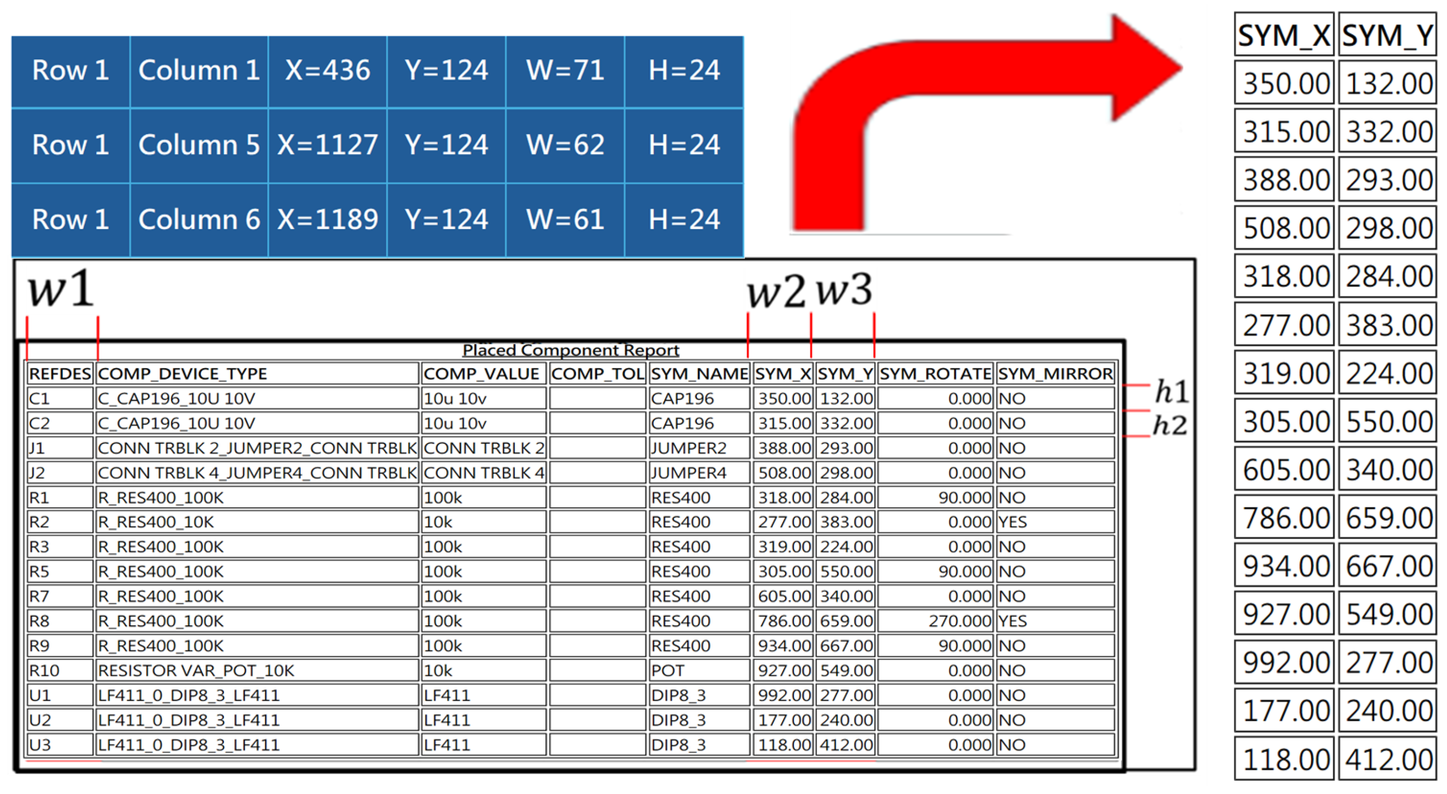
The merged horizontal lines are sorted from top to bottom according to their y-coordinates, while vertical lines are sorted from left to right according to their x-coordinates. The first row, which contains non-relevant information, is skipped. This study focuses on columns 1, 6, and 7, so only these columns are processed. The widths (w1, w2, w3) and heights (h1, h2, h15) of each rectangular cell, along with their coordinates (see Figure 8), are calculated. Based on this information, the images of the component coordinates are extracted and saved as JPG files.

4.3. Digit Segmentation

The digit segmentation method proposed in this study employs a pixel-scanning approach, in which the image is sequentially scanned from left to right and from top to bottom to isolate individual digits. In addition to segmenting, the spatial coordinates of each digit must be recorded to facilitate subsequent processing. This serves two primary purposes: (1) the x-coordinate of each digit is used to determine whether two digits are adjacent and should be merged into a single coordinate value; (2) the y-coordinate of each digit is used to identify the component to which the coordinate belongs. The top-left $(x_1,y_1)$ and bottom-right $(x_2,y_2)$ corners of each digit are stored in a three-dimensional array $pnt\left[k\right]\left[2\right]\left[2\right]$, where the $k$-th element represents the coordinate positions of a specific component, as expressed below:

$$\begin{gathered} pnt\left[k\right]\left[0\right]\left[0\right]=x_1;pnt\left[k\right]\left[0\right]\left[1\right]=y_1 \\ pnt\left[k\right]\left[1\right]\left[0\right]=x_2;pnt\left[k\right]\left[1\right]\left[1\right]=y_2 \end{gathered}$$

(6)

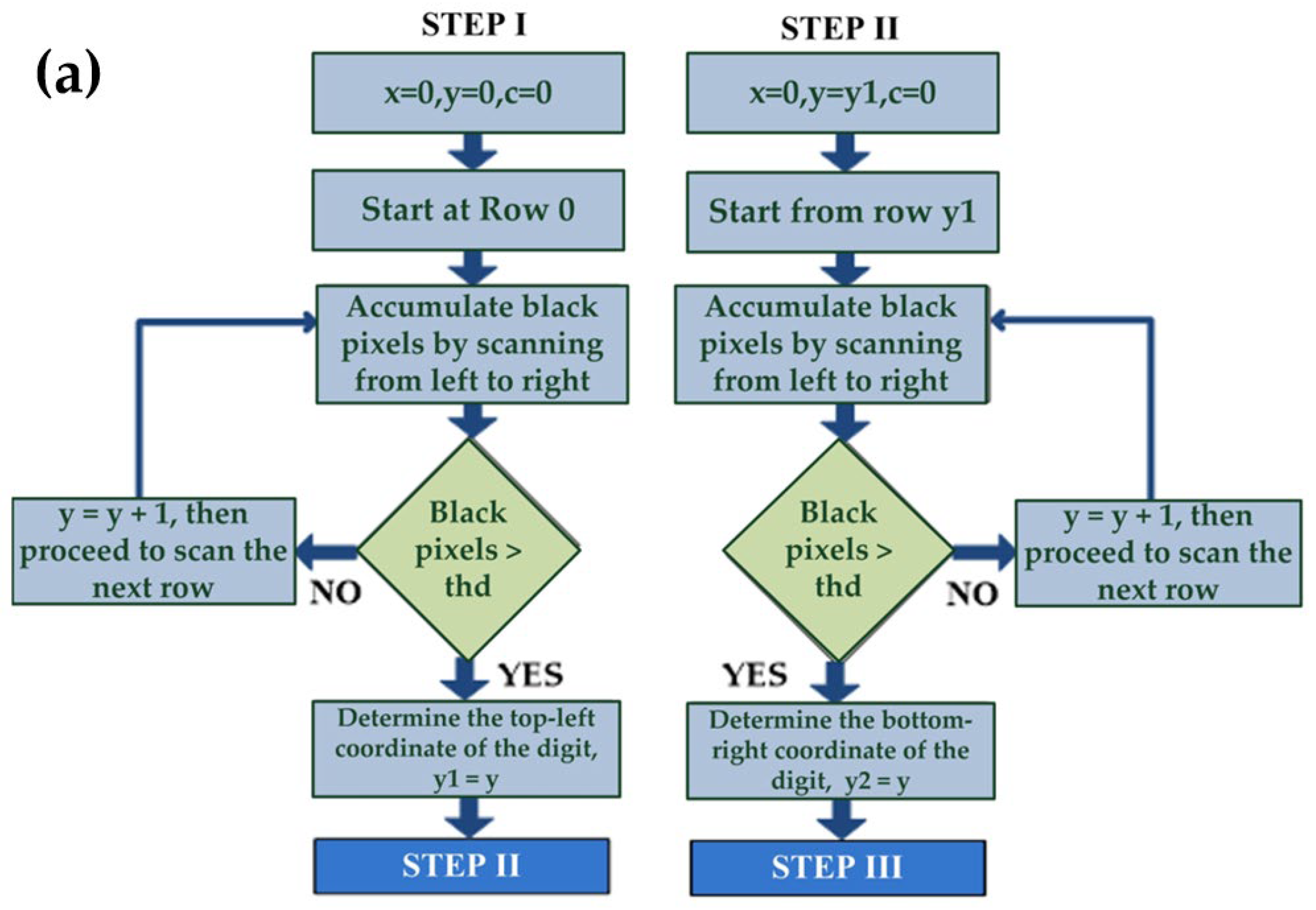
The flowchart of the pixel-scanning digit segmentation algorithm is illustrated in Figure 9.

[Step I] Three variables are initialized as follows: $x\left(col\right)=0, y\left(row\right)=0,c\left(pixel\right)=0$. Scanning begins from the top of the image $(y=0)$ and proceeds from left to right $(i=0,1,2,\dots ,col-1)$, covering a total of col pixels per row. If an entire horizontal line contains only white pixels or the number of black pixels is less than a predefined threshold $(c<thd)$, it is assumed that no digits are present in that row, and y is incremented to scan the next row. This left-to-right scanning continues until a row contains more black pixels than the threshold $(c\ge thd)$ is found, indicating the presence of digits. At this point, the current $y$ value is recorded as the upper vertical coordinate of the digit block, denoted as $y_1$, and scanning is temporarily halted.

[Step II] The three variables are reinitialized as follows: $x\left(col\right)=0,y\left(row\right)=y_1,c\left(pixel\right)=0$. Scanning resumes from the top of the digit block $(y=y_1)$, again proceeding from left to right ($i=0,1,2,\dots ,col-1)$, covering a total of col pixels per row. If the number of black pixels in a row is greater than or equal to the predefined threshold $(c\ge thd)$, the scanning process remains within the digit region, and y is incremented to continue scanning subsequent rows. This process repeats until a row is found where the number of black pixels falls below the threshold $(c\ge thd)$, indicating that the scan has entered a blank region with no digits. 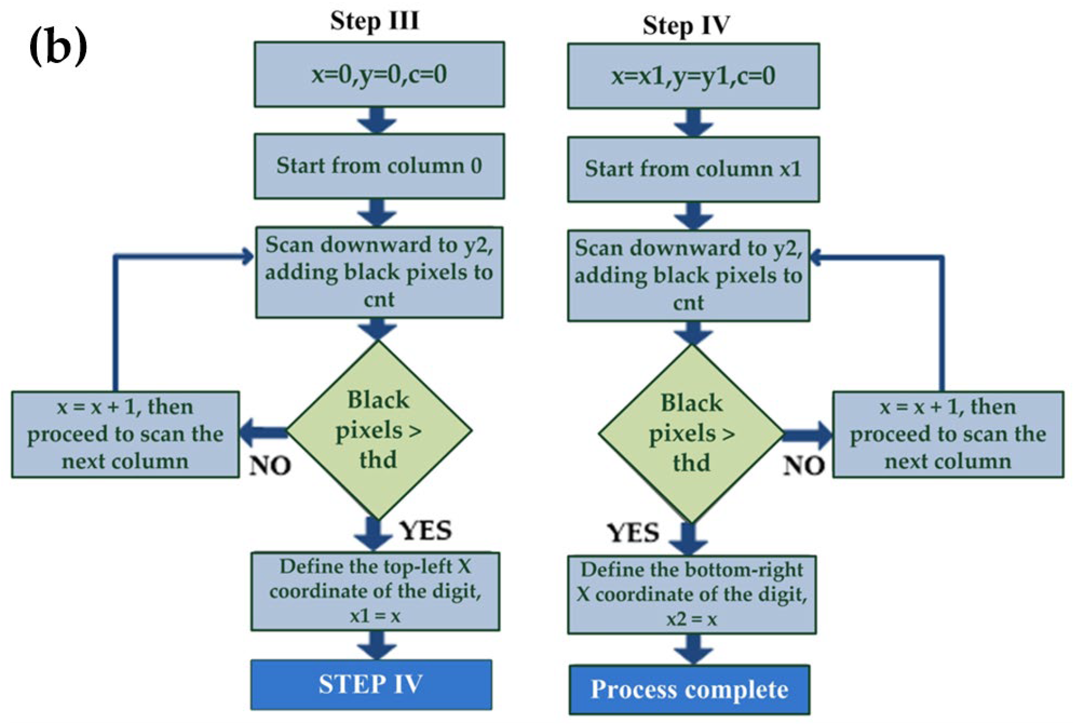The current $y$ value is then recorded as the lower vertical coordinate of the digit block, denoted as $(y=y_2)$, and the scanning process is terminated. The program flowcharts corresponding to Step I and Step II are shown in Figure 10a.

[Step III] Three variables are initialized as follows: $x\left(col\right)=0,y\left(row\right)=0 \mathrm{a}\mathrm{n}\mathrm{d} c\left(pixel\right)=0$. Scanning begins from the left side of the image $(x=0)$ and proceeds downward to the coordinate y₂ ($j=0,1,2,\dots ,y_2-1)$, scanning a total of $y_2$ pixels. If an entire vertical line contains only white pixels or the number of black pixels is less than a predefined threshold $(c<thd)$, it is assumed that no digits are present in that column, and $x$ is incremented to scan the next column. This top-to-bottom scanning process continues until a vertical line is found where the number of black pixels exceeds the threshold $(c\ge thd)$, indicating the presence of digits in that region. The current $x$ value is then recorded as the left horizontal coordinate of the digit block, denoted as $x_1$, and the scanning is temporarily halted.

[Step IV] The three variables are initialized as follows: $x\left(col\right)=x_1,y\left(row\right)=0 \mathrm{a}\mathrm{n}\mathrm{d} c\left(pixel\right)=0$. Scanning starts from the left side of the digit block $(x=x_1)$ and again proceeds downward to the $y_2$ $(j=0,1,2,\dots ,y_2-1)$, covering a total of $y_2$ pixels. If the number of black pixels in a vertical line exceeds the predefined threshold $(c\ge thd)$, it is assumed that the scanning line intersects with the digits, and $x$ is incremented to continue scanning the next column. This top-to-bottom process is repeated until a vertical line is found where the number of black pixels falls below the threshold $(c<thd)$, indicating that the vertical line has moved into a blank area with no digits. The current x value is recorded as the right horizontal coordinate of the digit block, denoted as $x_2$, and the scanning process is terminated. The program flowcharts corresponding to Step III and Step IV are shown in Figure 10b.

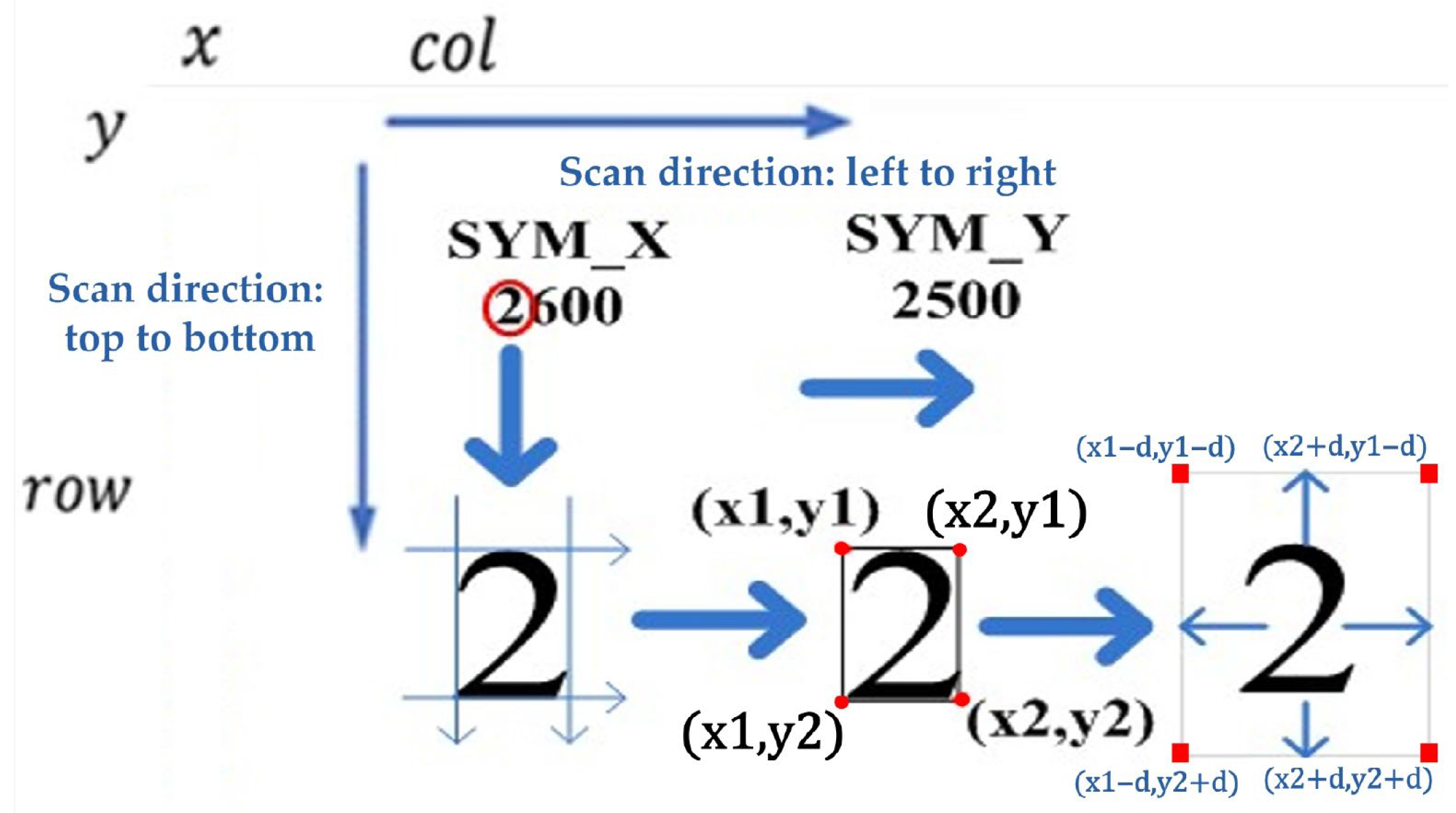
[Step V] From Steps I–IV, the digit “2” located at the top-left corner of the image in Figure 11 can be extracted. The coordinates of the top-left corner (x₁,y₁) and bottom-right corner (x₂,y₂) of the digit are stored in a three-dimensional array pnt[k][2][2], where k denotes the index of the extracted digit. At this stage, the algorithm segments the digit strictly according to its four corner points, resulting in the digit occupying the entire bounding region, which may degrade the performance of subsequent neural-network recognition. To enhance image quality, the segmentation boundaries are expanded by a distance d in all four directions-top, bottom, left, and right-before cropping the digit region.

[Step VI] After extracting the digit located at the top-left corner of the image, the segmented digit is saved as an individual image file. Using the top-left (x₁,y₁) and bottom-right (x₂,y₂) coordinates, a white block of the same size is created to overwrite the extracted region in the original image. By repeating Steps I–IV, the algorithm sequentially extracts the remaining digits one by one until all have been processed.

4.4. Digit Recognition

4.4.1. Training Dataset

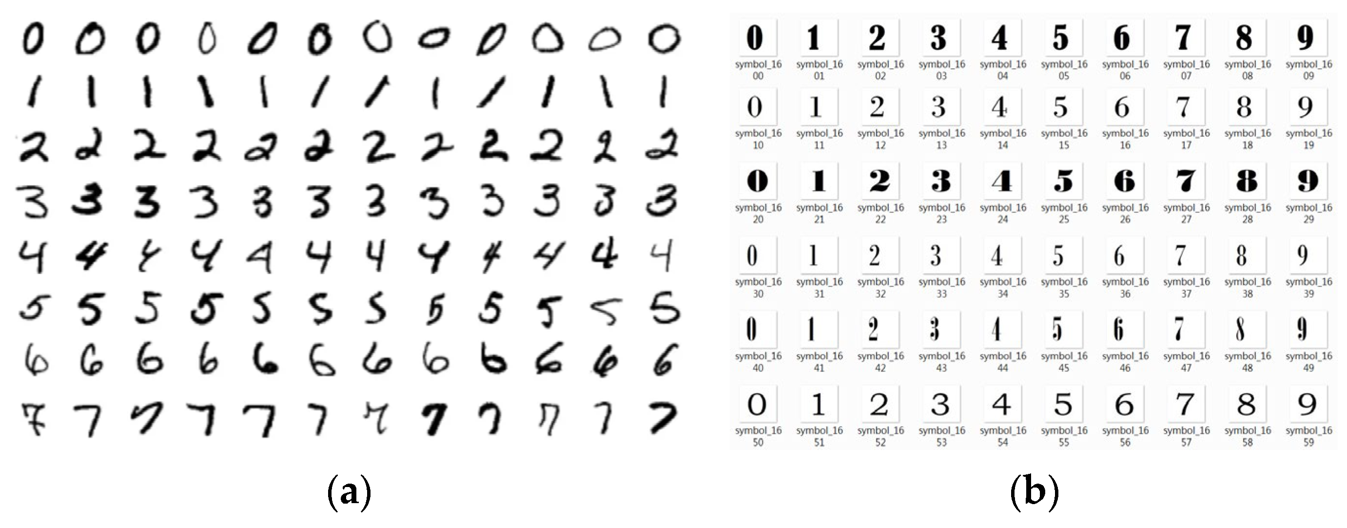
The MNIST handwritten digit dataset [31], collected by LeCun and colleagues, comprises 60,000 training samples and 10,000 testing samples. Each sample includes an image of a handwritten digit and its corresponding label. The images are 28 × 28 pixels in size (784 pixels in total) and are binary black-and-white, making this dataset well suited for model training and performance evaluation, as illustrated in Figure 12a. In this study, the 60,000 MNIST training samples were divided into 80% (48,000 samples) for training and 20% (12,000 samples) for validation. Considering the substantial differences between handwritten digits and computer-generated fonts extracted from PCRs, an additional dataset of Arabic numeral images (0–9), referred to as the CFONT dataset, was established, as shown in Figure 12b. The CFONT dataset consists of 4580 images generated by rendering digits 0–9 using 458 distinct TrueType/OpenType font files. For each font, one image is generated for each digit from 0 to 9, resulting in a total of 458 × 10 = 4580 images. This construction ensures systematic coverage of font-style variations while maintaining a fixed one-to-one correspondence between each font and the ten numeral classes. In this work, the digit dataset was self-constructed rather than taken from public repositories. A Python-based generator was used to render the digits, followed by alignment correction and normalization to 28 × 28 px to prepare the inputs for CNN inference. These images were then combined with the MNIST handwritten dataset to train the neural network and to evaluate its recognition accuracy under different architectural configurations.

4.4.2. Multilayer Perceptron (MLP)

MLP is a feedforward artificial neural network composed of multiple layers of fully connected neurons. It is widely used for classification and regression tasks and serves as one of the fundamental models in deep learning. In this study, an MLP model is employed for digit recognition. The input layer consists of 784 neurons, corresponding to a 28 × 28 grayscale image that is flattened into a one-dimensional array. The hidden layer contains 256 neurons, each computes a weighted sum of the previous layer’s outputs followed by an activation function. The output layer comprises ten neurons, representing the predicted digits from 0 to 9. The total number of trainable parameters in the MLP architecture is calculated as follows:

$$256\times 784+256+256\times 10+10=200960+2570=203530$$

(7)

4.4.3. Convolutional Neural Network (CNN)

CNNs are characterized by the use of convolutional and pooling layers. The convolutional layer applies convolutional kernels (or filters) to the input data to extract discriminative features such as edges, textures, and shapes. This structure enables the network to automatically learn hierarchical representations of image features at multiple levels. The pooling layer, which typically follows each convolutional layer, reduces the spatial dimensions of the feature maps, thereby decreasing computational complexity and mitigating overfitting.

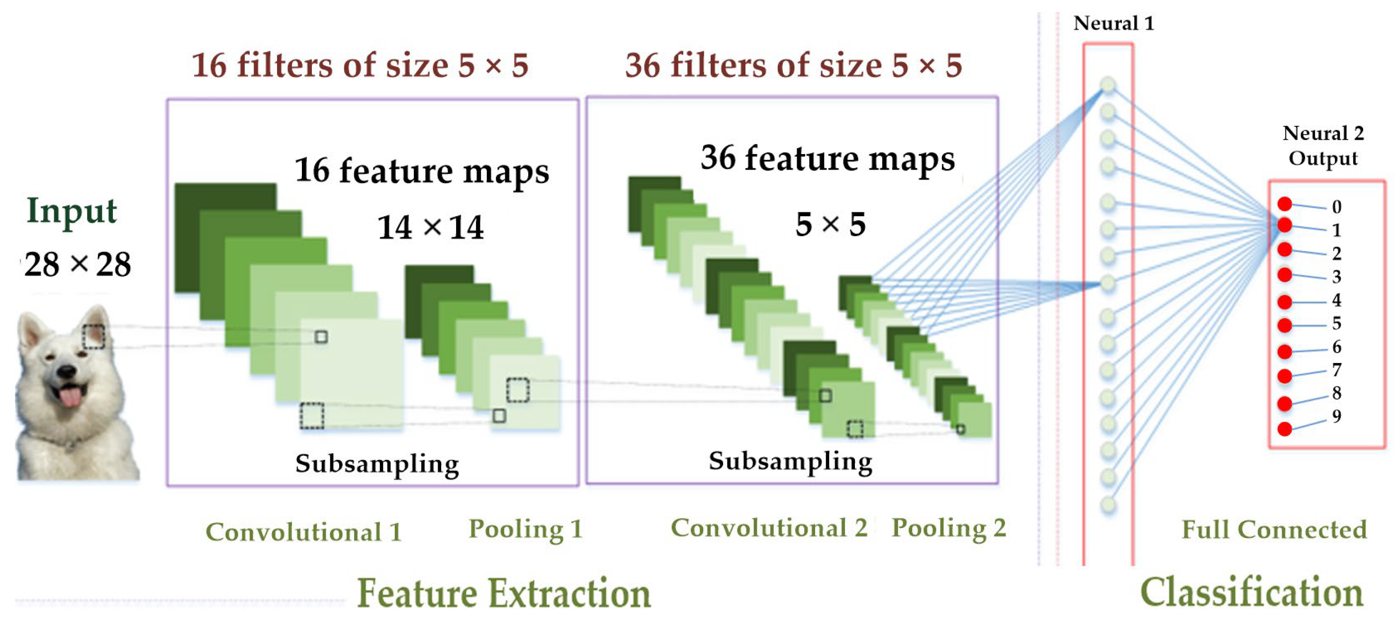
The CNN architecture used in this study is illustrated in Figure 13. It consists of two convolutional–pooling stages followed by fully connected layers. The first convolutional layer takes an input image of 28 × 28 pixels and applies 16 filters of size 5 × 5. In total, 416 weights are updated simultaneously, calculated as 25 × 16 + 16. These filters produce 16 feature maps of the same size (28 × 28). Pooling Layer 1 performs the first downsampling operation, reducing the feature maps from 16 × 28 × 28 to 16 × 14 × 14.

The second convolutional layer processes the 14 × 14 input images using 36 filters of size 5 × 5, resulting in 14,436 trainable weights, computed as 25 × 36 × 16 + 36. This layer outputs 36 feature maps, each of size 14 × 14. Pooling Layer 2 then performs the second downsampling operation, reducing the feature maps to 36 × 7 × 7.

A dropout layer with a rate of 0.25 is incorporated after Pooling Layer 2 to randomly deactivate 25% of the neurons during each training iteration, thereby reducing the risk of overfitting. The subsequent flatten layer converts the output of Pooling Layer 2, which consists of 36 feature maps of size 7 × 7, into a one-dimensional array of 1764 elements corresponding to 1764 input neurons. A fully connected hidden layer with 128 neurons is then constructed, yielding a total of 225,920 trainable parameters (1764 × 128 + 128).

To further mitigate overfitting, another dropout layer with a rate of 0.5 is incorporated, randomly deactivating 50% of the neurons during each training iteration. The output layer consists of 10 neurons, corresponding to the classification of digits from 0 to 9, and includes 1290 trainable parameters (128 × 10 + 10). In total, the proposed CNN architecture contains 242,062 trainable parameters, encompassing all convolutional, fully connected, and output layers. For clarity and reproducibility, the detailed architecture and parameter configuration of the CNN model used in this study are summarized in

Table 1. CNN model parameters.

ID	Layer Name	Dimension	Parameters
1	Conv2D-1 (3 × 3, 16 filters)	28 × 28 × 16	416
2	MaxPooling2d-1 (2 × 2)	14 × 14 × 16	0
3	Conv2D-2 (3 × 3, 36 filters)	14 × 14 × 36	14,436
4	MaxPooling2d-2 (2 × 2)	7 × 7 × 36	0
5	Dropbox	7 × 7 × 36	0
6	Flatten	1764	0
7	Dense-1 (128 units)	128	225,920
8	Dropbox	128	0
9	Dense-2 (128 units)	10	1290
10	Total	−	242,062

.

4.4.4. MLP Trained on MNIST Dataset

Before training, the MNIST dataset is preprocessed by transforming each 28 × 28 grayscale image into a 784-dimensional feature vector and converting the corresponding labels into one-hot encoded representations. The processed data is then fed into the Multilayer Perceptron (MLP) model for training. The trained model is subsequently used to predict both handwritten digits and computer-generated fonts. In this work, predictions are performed on five different computer fonts, namely Aptos, Neue Haas Grotesk Text Pro Black, Goudy Stout, Aharoni, and BiauKai, using a total of 49 test images in the trained MLP model. The model achieves an average recognition accuracy of approximately 70%. However, the three-layer MLP model fails to reach the desired level of accuracy, primarily due to its limited capacity to extract spatial features.

4.4.5. CNN Trained on MNIST Dataset

The MNIST dataset was preprocessed and subsequently used to train the convolutional neural network (CNN) model. To evaluate its generalization performance o, a set of 49 test images rendered in five distinct computer fonts, namely Aptos, Neue Haas Grotesk Text Pro Black, Goudy Stout, Aharoni, and BiauKai, was used for testing. The trained CNN model achieved an average recognition accuracy of approximately 90%, demonstrating strong robustness to variations in font style. Under identical training conditions, the CNN significantly outperformed the MLP model.

4.4.6. CNN Trained on MNIST + CFONT Datasets

In addition, this study used the MNIST handwritten digit dataset as the foundation, supplemented by the self-constructed CFONT computer font dataset, resulting in a total of 64,580 images as training samples for the CNN model. The trained model was evaluated using 49 test images rendered in five different computer fonts—Aptos, Neue Haas Grotesk Text Pro Black, Goudy Stout, Aharoni, and BiauKai—and achieved an average recognition accuracy of approximately 92%. Compared with the CNN trained solely on the MNIST dataset (≈90% accuracy), the inclusion of CFONT data yielded a modest improvement in recognition performance, indicating that combining handwritten and computer-font samples enhances feature diversity and slightly improves generalization.

4.4.7. CNN Trained on CFONT Dataset

Finally, only the self-collected CFONT dataset, consisting of 4580 Arabic numeral images (0–9) using different computer fonts, was used to train the CNN model parameters. The trained CNN model was evaluated using 49 test images rendered in five different computer fonts: Aptos, Neue Haas Grotesk Text Pro Black, Goudy Stout, Aharoni, and BiauKai. The experimental results demonstrated that when trained exclusively on the CFONT dataset, the CNN model achieved a recognition accuracy of approximately 98%, thereby meeting the expected performance target.

When the CNN model was trained exclusively on the CFONT dataset, its recognition accuracy reached 98%, representing a substantial improvement compared with the CNN trained on MNIST alone (≈90%) and the CNN trained on the combined MNIST + CFONT datasets (≈92%). This result indicates that the computer-font training data are more consistent with the characteristics of the rasterized PCRs used in this study, enabling the network to extract more representative font features. 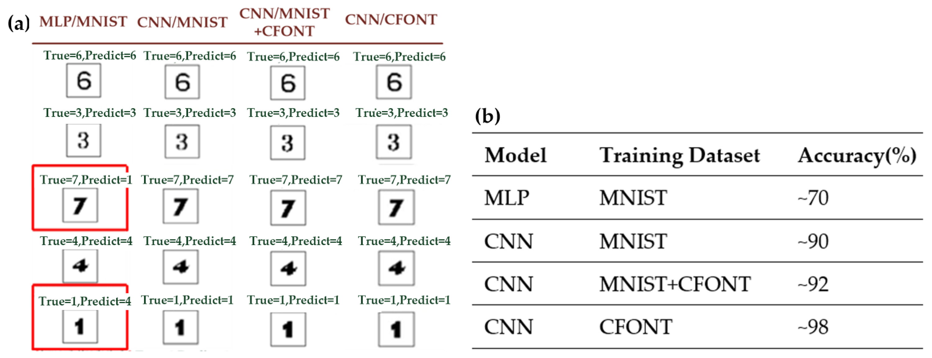Figure 14a presents a comparative analysis of recognition performance across four training configurations: MLP (MNIST), CNN (MNIST), CNN (MNIST + CFONT), and CNN (CFONT). The table illustrates recognition results for five representative font styles—Aptos, Neue Haas Grotesk Text Pro Black, Goudy Stout, Aharoni, and BiauKai—arranged from top to bottom. As highlighted by the red boxes, the MLP model trained solely on MNIST misclassifies digits from visually similar font types (e.g., “7” as “1” and “1” as “4”). In contrast, the CNN model trained with CFONT data achieves the best performance, accurately recognizing unseen font styles and maintaining consistent predictions across diverse typographic variations.

Figure 14 representative digit recognition results under different model architectures and training datasets. The left panel shows qualitative prediction examples, where misclassified samples are highlighted with red boxes. The right panel summarizes the corresponding recognition accuracies for each model–dataset combination.

4.5. Hand Gesture Recognition Using MediaPipe

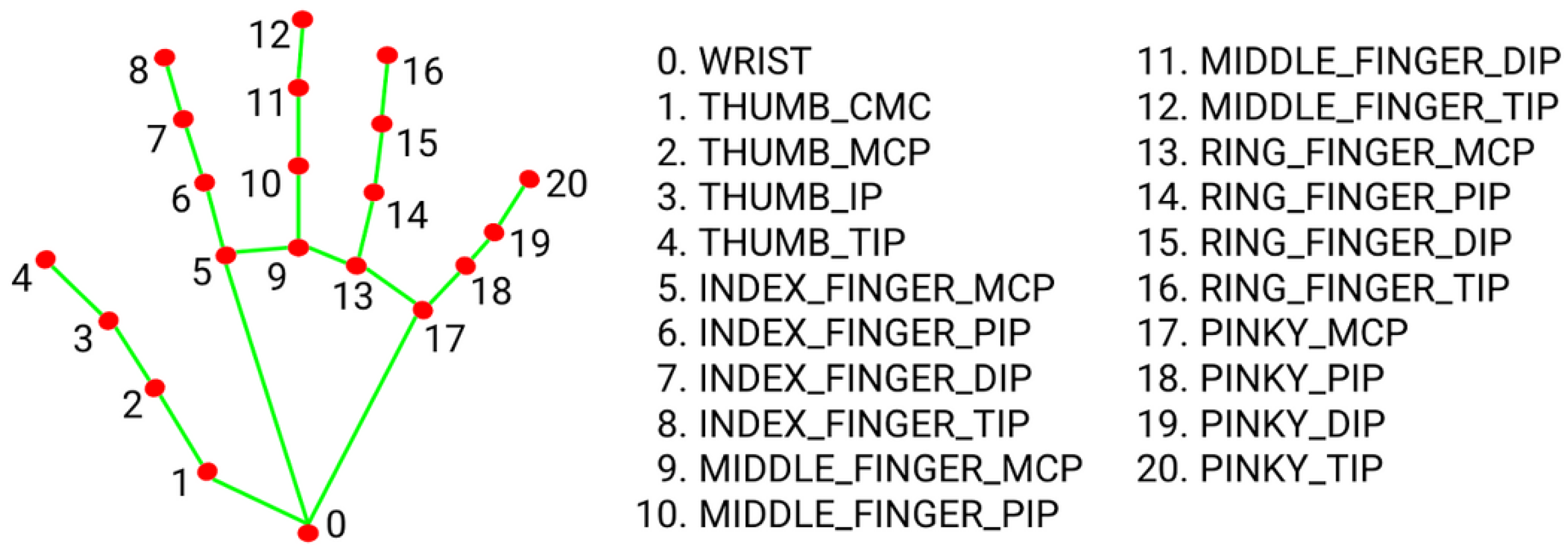
In this study, the hand detection solution provided by the MediaPipe framework was utilized. Images were captured by the system’s camera and processed using the open-source hand detection module of MediaPipe. This module applies machine learning techniques to detect hand regions and accurately estimate the 21 hand-joint landmark coordinates from a single image frame. The extracted landmark positions were subsequently used for hand gesture and posture recognition. In the proposed system, the index fingertip position serves as the reference point for determining four directional commands, which are forward, backward, left, and right, to achieve fine motion control of the XY platform. MediaPipe identifies 21 key points on the hand, where landmark point 8 corresponds to the index fingertip, as illustrated in Figure 15. Once the fingertip is localized, users can intuitively observe the real-time hand gesture tracking results on the display. To capture the continuous movement of gestures, the system records the index fingertip position in each video frame. When both the current and previous frame positions are available, an arrowed line is drawn between the two consecutive points. This visualization not only depicts the trajectory of fingertip motion but also provides the foundation for analyzing movement direction in subsequent processing stages.

Subsequently, the system compares the displacement differences between the current and previous frames along the horizontal (X-axis) and vertical (Y-axis) directions. If the displacement in the horizontal direction exceeds that in the vertical direction, the movement is classified as left or right; otherwise, it is identified as forward or backward. To minimize misclassification caused by minor hand tremors while maintaining responsive control, a displacement threshold is introduced to trigger directional motion commands. In practice, the selection of the gesture displacement threshold represents a trade-off between suppressing unintended micro-movements caused by hand jitter and maintaining responsive user control. If the threshold is set too small, involuntary hand tremors may easily trigger unintended platform movements. Conversely, an excessively large threshold may lead to noticeable response delays and reduced control comfort. Based on iterative empirical testing under the experimental setup used in this study, a displacement threshold of 40 pixels was found to provide stable and intuitive interaction behavior.

5. Experimental Results

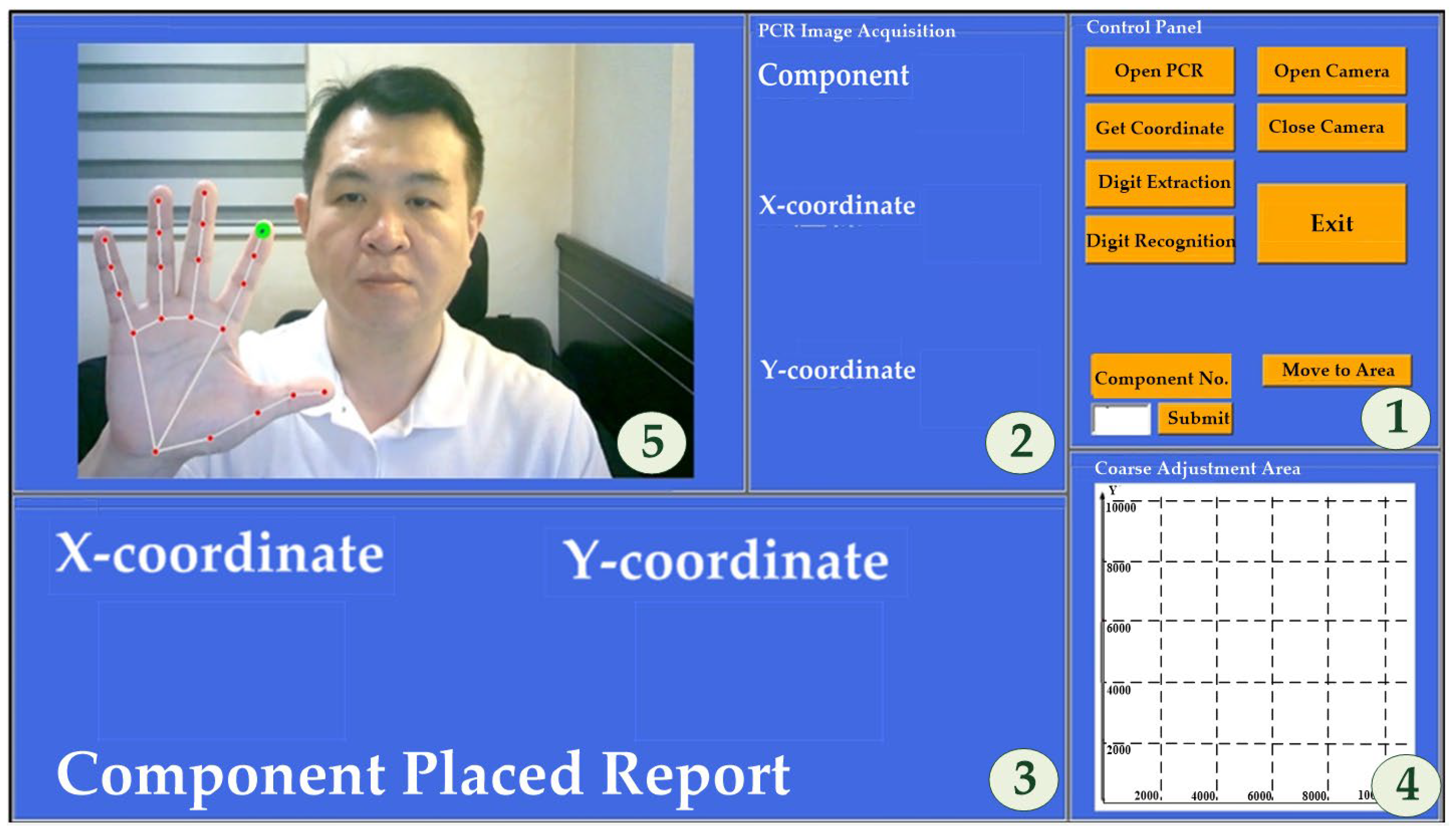
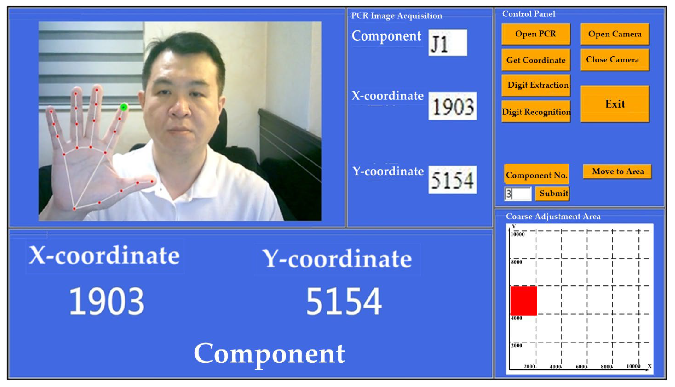
In this study, a graphical user interface (GUI) was developed using the Tkinter library (Python standard library, Python Software Foundation, Wilmington, DE, USA) in Python. Tkinter serves as the standard graphical toolkit for Python, and by employing the PanedWindow function, the interface can display multiple window frames concurrently. Figure 16 illustrates the layout of the designed GUI. The interface simultaneously displays the component coordinate positions extracted from the PCR on a text window and visualizes both the movement area of the XY platform during the coarse adjustment stage and the hand gesture operations during the fine adjustment stage. The GUI comprises five window frames (labeled with circled numbers 1–5 in Figure 16), each dedicated to a specific system function: (1) Control Panel, (2) PCR Image Acquisition, (3) PCR Component Coordinates, (4) Coarse Adjustment Area, and (5) Fine Adjustment Gesture Recognition. The system functionalities and operational procedures are summarized as follows.

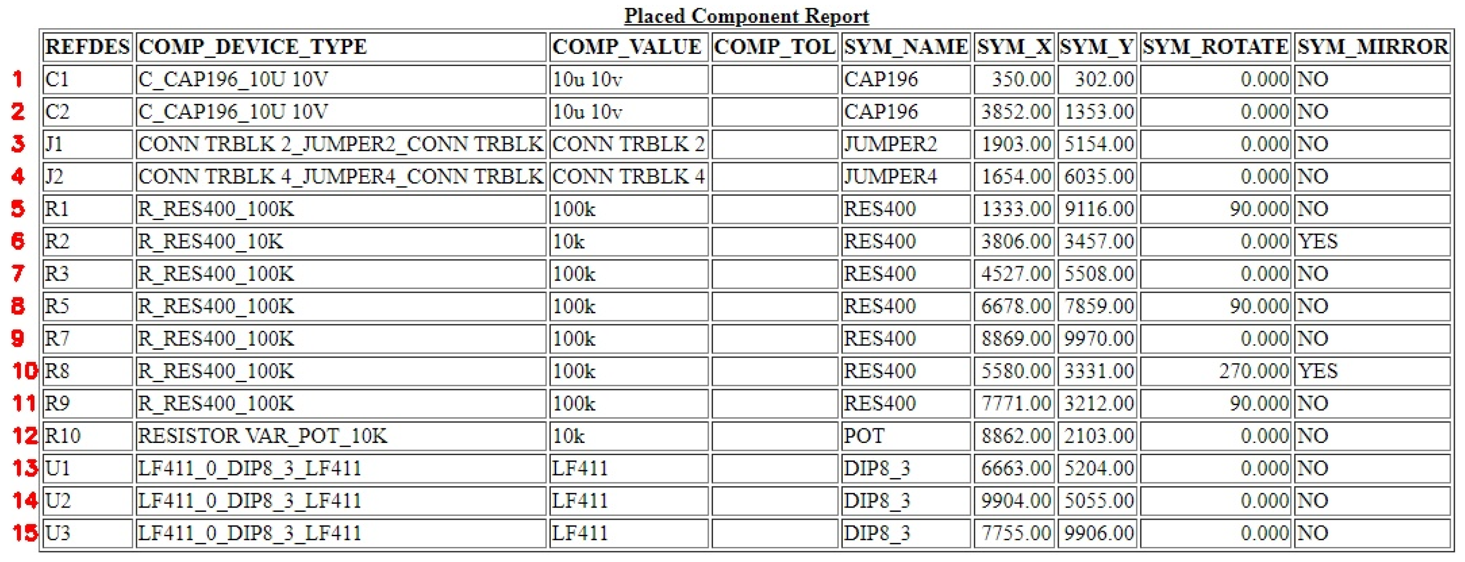
[Step 1] By clicking the “Open PCR” button on the control panel, users can select and open a Placed Component Report (PCR) file exported from a PCB layout tool. The system incorporates the Selenium library within the Python environment to convert the PCR document in HTML format into a JPG image, with component identifiers automatically annotated on the converted image, as illustrated in Figure 17.

[Step 2] By clicking the “Capture Coordinates” button on the control panel, the system executes a Hough-transform-based line detection algorithm to address the following issues: (1) merging table borders formed by closely spaced double solid lines into a single line; (2) calculating the row heights (h1, h2…h15); (3) determining the column widths (w1, w2, w3); and (4) filtering and computing the valid field widths and heights. Based on the PCR table format shown in Figure 17, the system captures images from columns 1, 6, and 7, resulting in 45 image files stored in a designated folder.

[Step 3] By clicking the “Digit Segmentation” button on the control panel, the system applies a pixel-scanning method to perform digit segmentation on 45 extracted image files. Each image is scanned from left to right and top to bottom to isolate individual digits. In addition to segmentation, each digit is assigned a positional index within the image to facilitate the subsequent reconstruction of component coordinates on the PCB. The segmented digit images are then saved into a designated directory.

[Step 4] By clicking the “Digit Recognition” button on the control panel, the system utilizes the CFONT dataset, which contains 4580 computer-generated images of Arabic numerals (0–9), to train a CNN-based recognition model. The trained model achieves a recognition accuracy exceeding 96%. After recognition, the system merges the identified digits to reconstruct the coordinate positions of each component on the PCB layout.

[Step 5] In the control panel, users enter “3” in the “Component Number” field and click the “Submit” button. By subsequently clicking “Capture Coordinates,” the component field in the PCR image acquisition window displays J1, while the X-coordinate and Y-coordinate fields show 1903 and 5154, respectively, as illustrated in Figure 18. Using the Hough Transform, the positions, column widths, and row heights of the three image regions corresponding to the J1 component in the PCR form (Figure 18) are computed. Based on this information, the system automatically displays the three associated images within their respective interface windows. The extracted spatial parameters of component J1 are listed in

Table 2. Extracted positional information of component J1 from the PCR.

ID	Row Index	Column Index	X (px)	Y (px)	Width (px)	Height (px)
J1	3	1	436	172	71	24
J1	3	6	1127	172	62	24
J1	3	7	1189	172	61	24

, which include the X–Y positions and the corresponding width (W) and height (H) values of the relevant table fields.

[Step 6] By sequentially clicking the “Digit Segmentation” and “Digit Recognition” buttons on the control panel, the system first performs digit segmentation using a pixel-scanning method, followed by digit recognition through the trained CNN model. After processing, The PCR Component Coordinates window displays the X-coordinate (1903) and the Y-coordinate (5154) for the selected component.

[Step 7] By clicking the “Move to Area” button on the control panel, the Coarse Adjustment Movement Area window is divided into a 5 × 5 grid. A red block marks the location of the J1 component, indicating the target area to which the XY platform rapidly moves during the coarse-adjustment stage.

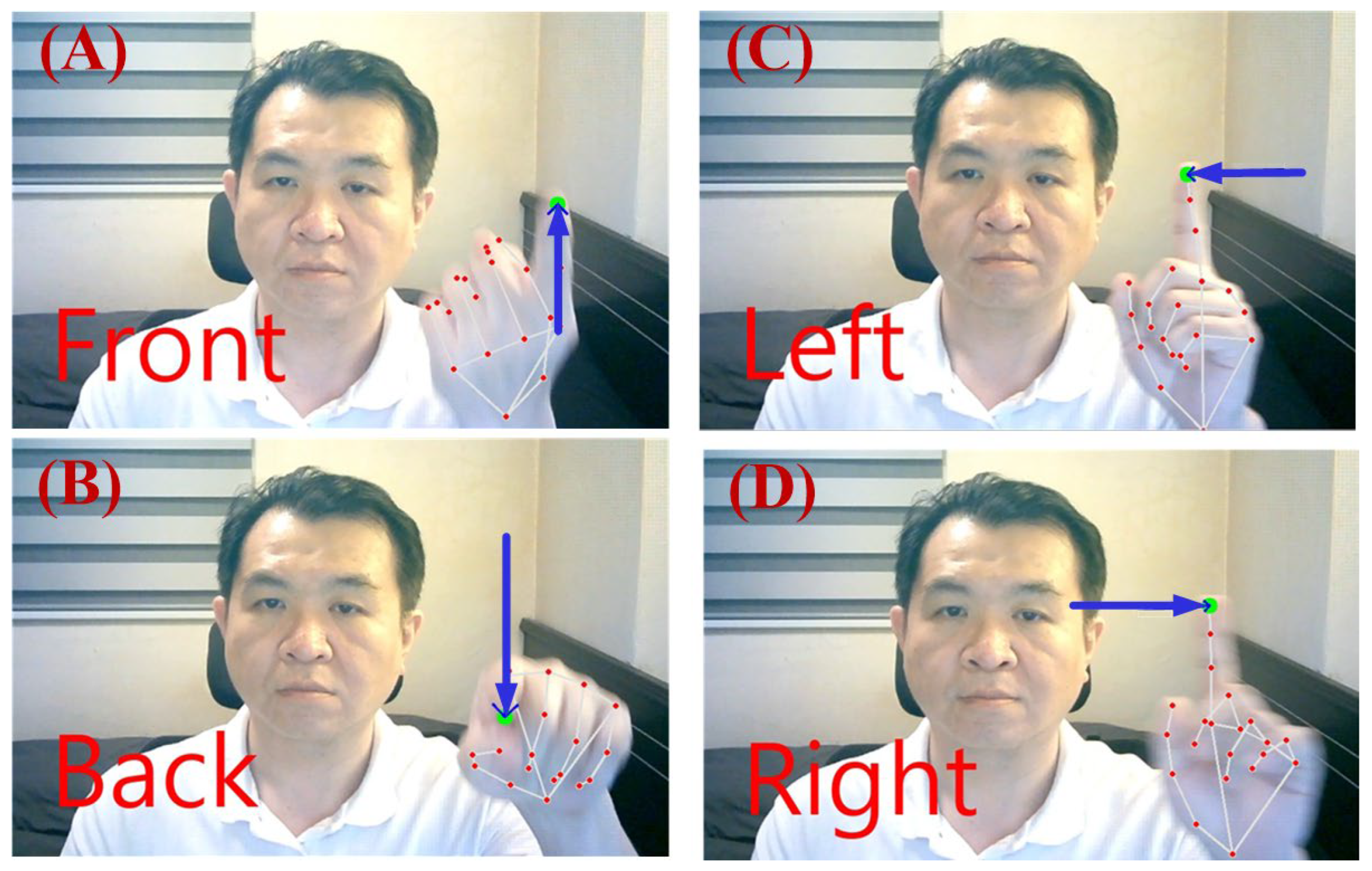
[Step 8] By clicking the “Open Camera” button on the control panel, the MediaPipe-based gesture recognition function is activated, and the XY platform enters the fine-tuning stage. The fine-tuning gesture recognition window displays the real-time camera stream and continuously captures the coordinates of 21 hand landmarks. When the user opens their palm, MediaPipe detects the open-hand gesture and begins tracking the position of the eighth landmark point, as illustrated in Figure 19. If the Y-coordinate of the eighth landmark continuously increases while the X-coordinate remains constant, the system interprets this motion as an upward movement of the dual-axis linear stage by 0.05 mm per micro-step, as shown in Figure 19A. Conversely, if the Y-coordinate decreases while the X-coordinate remains constant, the system moves the stage downward by the same increment, as illustrated in Figure 19B. Similarly, when the X-coordinate decreases with a constant Y-coordinate, the system drives the stage leftward by 0.05 mm per micro-step, as depicted in Figure 19C; if the X-coordinate increases while the Y-coordinate remains constant, the stage moves rightward, as shown in Figure 19D.

To further interpret the gesture-triggered behavior shown in Figure 19, rather than relying on an absolute pixel value, the threshold is formulated in a frame-normalized manner to improve resolution independence. Let $W$ and $H$ denote the width and height of the camera frame in pixels. A gesture-triggering condition is defined as $\left|∆x\right|/W>{\tau }_x$ or $\left|∆y\right|/H>{\tau }_y$, where ${\tau }_x$ and ${\tau }_y$ are the normalized thresholds for horizontal and vertical motion, respectively. Under the experimental setup used in this study, with a camera resolution of 1920 × 1080 pixels, the empirically selected threshold corresponds to approximately 2.1% of the frame width in the horizontal direction and 3.7% of the frame height in the vertical direction, which is equivalent to a displacement of 40 pixels. This formulation preserves the original system behavior while providing a more general and scalable interpretation of the gesture threshold across different camera resolutions. Once the displacement magnitude satisfies the triggering condition, the system identifies the intended movement direction and immediately transmits the corresponding control command to the ATmega168 command-transmission board, which then forwards it via a Bluetooth module to the ATmega168 motion-control board for fine adjustment of the XY platform position. In addition to executing the command, the detected direction is simultaneously displayed in red text at the upper-left corner of the real-time video feed, as illustrated in Figure 19, where the real-time gesture-triggered fine adjustment behavior is demonstrated. This real-time visual feedback allows users to promptly adjust their hand gestures, thereby ensuring accurate and reliable non-contact control. Compared with conventional button-based control, the proposed gesture-driven fine-tuning interface offers a non-contact and safer operation mode suitable for industrial inspection environments. Figure 20a illustrates the hardware configuration of the proposed optical inspection system. The Raspberry Pi transmits the extracted positioning coordinates wirelessly via Bluetooth to the ATmega168 microcontroller. Upon receiving the coordinates, the ATmega168 immediately drives the stepper motors along the X- and Y-axes, moving the dual-axis linear stage to the designated region and thereby completing the coarse positioning of the XY platform. Figure 20b presents the main hardware components of the system, including (1) the XY linear stage, (2) the ATmega168 control board, (3) the TB6600 stepper motor drivers, and (4) the DC power supply.

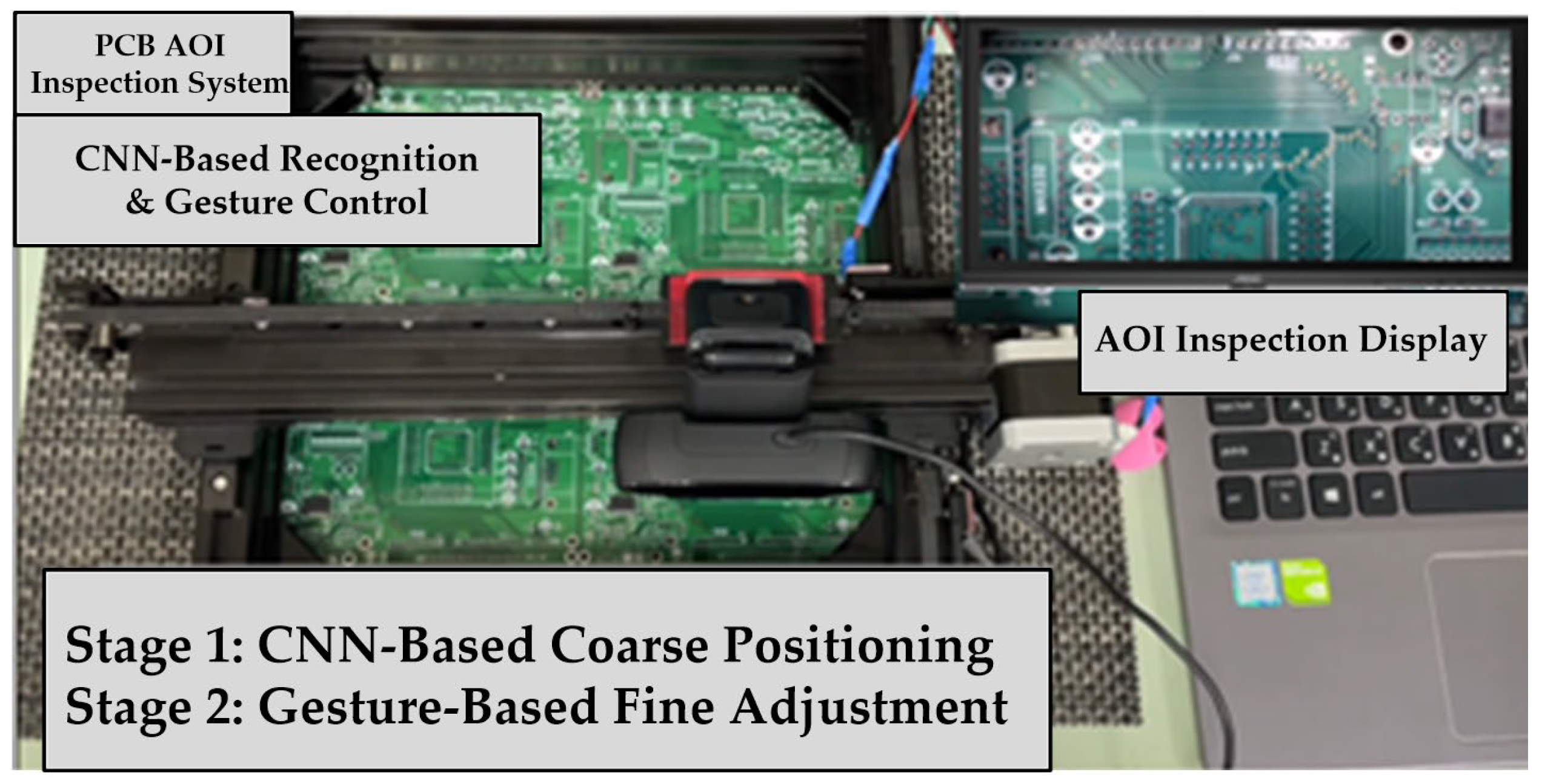
After the camera is activated, the PCB image is displayed in real time on a large AOI monitor, allowing operators to conveniently perform visual inspection of solder joints. During the inspection process, the operator can further adjust the position of the XY platform in the up, down, left, and right directions using hand gesture trajectories. This gesture-based interaction enables fine positioning of the camera relative to the target coordinates, facilitating accurate alignment during inspection. The experimental results demonstrate the feasibility and effectiveness of the proposed two-stage positioning strategy for PCB solder joint inspection, as illustrated in Figure 21.

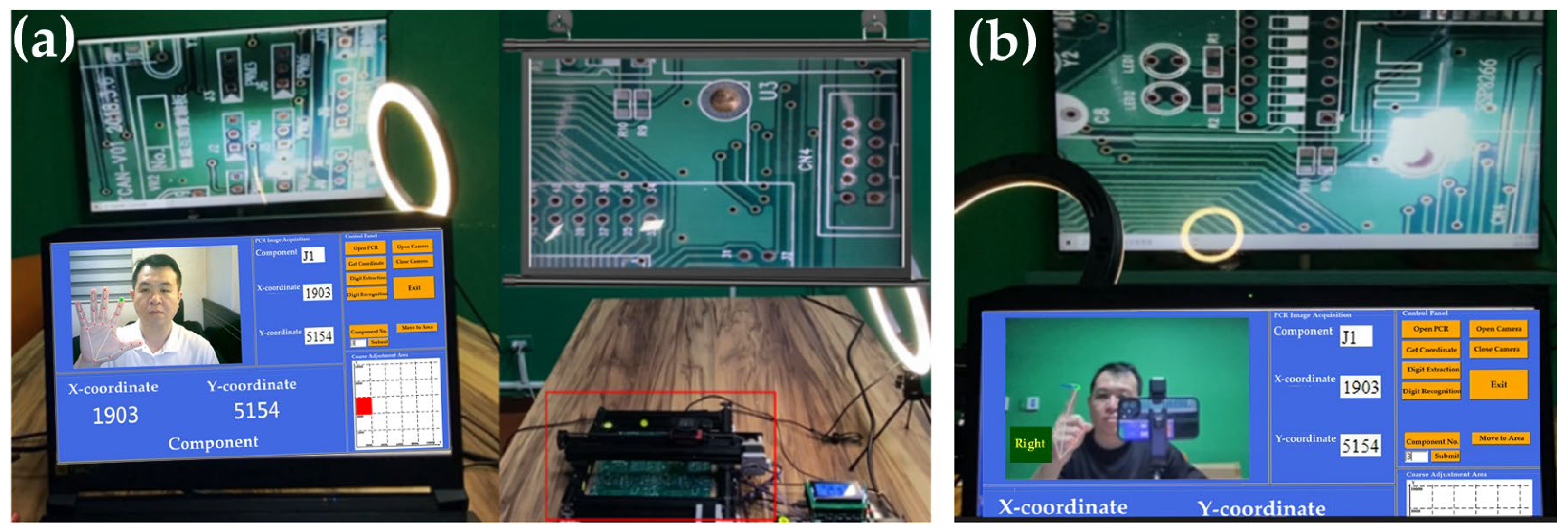
Figure 22 presents the experimental setups corresponding to the coarse and fine adjustment stages. In the coarse adjustment stage (Figure 22a), the projected PCB layout is aligned with the target region on the XY platform to achieve rapid region-level positioning. In the fine adjustment stage (Figure 22b), the system performs incremental movements with a step size of 0.05 mm, enabling refined alignment between the PCB and the camera imaging area.

6. Conclusions and Future Research

This paper presents a semi-automated optical positioning and inspection system for printed circuit boards (PCBs), designed to operate with layout reports exported from mainstream PCB design tools. The developed platform combines an XY dual-axis linear motion system, a camera module, and CNN-based image recognition to accurately extract component coordinates from PCR layout reports. These coordinates are transmitted via Bluetooth to control stepper motors, enabling precise positioning and visual inspection support. Additionally, MediaPipe-based hand gesture recognition and air-writing interaction are incorporated to provide an intuitive and contact-free control interface. The system displays real-time inspection results on a large monitor, significantly enhancing both inspection efficiency and accuracy. The proposed approach not only reduces manual labor but also provides an efficient and scalable framework for smart manufacturing and automated production lines. The primary contribution of this work lies in enabling automated, tool-independent coordinate extraction and CNN-based numeric reconstruction for AOI-oriented applications, effectively overcoming the limitations of coordinate mapping and manual operation in traditional AOI systems. The proposed platform therefore offers a practical and deployable solution for intelligent PCB inspection.

Despite the effectiveness of the proposed positioning-assisted inspection framework, several limitations should be noted. First, the system is not intended to replace fully automated, high-precision closed-loop AOI systems. The proposed approach emphasizes robust region-level positioning combined with human-in-the-loop fine adjustment, rather than exact coordinate convergence at the sub-millimeter level. Second, the extraction of component coordinates relies on the visual structure of EDA/PCRs. Although the proposed method is designed to handle visually rendered tables, reports with extremely compact layouts, irregular column spacing, or very small row heights may increase the difficulty of accurate coordinate extraction and require additional parameter tuning. Third, the gesture-based fine adjustment mechanism depends on the camera configuration and imaging resolution. While a frame-normalized formulation has been adopted to improve generality, optimal interaction behavior may still vary across different hardware setups and viewing distances. Finally, the effective inspection coverage is constrained by the physical travel range of the XY platform. Since PCB sizes may vary across inspection tasks, very large boards may exceed the platform workspace, resulting in some components being partially or fully outside the observable region. These limitations primarily reflect practical engineering constraints rather than fundamental shortcomings of the proposed approach and provide guidance for future system scaling and deployment.

Future research will focus on the following directions: (1) enhancing the recognition accuracy and computational efficiency of CNN models to strengthen defect detection performance; (2) applying real-time image processing and reinforcement learning techniques to improve the system’s adaptability to PCB variations; (3) integrating multimodal sensing technologies to enhance the detection capability for different materials and structures while reducing false detection rates; (4) adopting cloud and edge computing architectures to enable real-time data analysis and remote monitoring; (5) integrating MES and ERP systems to achieve real-time AOI data feedback and production management synchronization, thereby promoting smart factory operations and Industry 4.0 development; and (6) employing zoom-capable, high-resolution camera modules to improve image detail observation and micro-defect detection performance. Furthermore, the proposed technologies can be extended to contactless gesture recognition and air-writing interfaces that combine computer vision and deep learning for automatic target and defect identification, thereby achieving high-precision automated manufacturing and advancing intelligent production capabilities.