Assessing the White-in-Time Stochastic Forcing in Resolvent Prediction of Velocity and Pressure for Turbulent Channel Flow

Abstract

Research on the frequency spectra of velocity and pressure fluctuations in turbulent channel flow is central to applications in petroleum engineering, including pipeline transport efficiency, erosion prediction, and flow-induced vibration in wellbores and surface facilities. Direct numerical simulation at high Reynolds numbers remains prohibitively expensive, motivating the use of resolvent analysis as a computationally efficient alternative. The resolvent analysis, formulated from the linearized Navier–Stokes equations, relies on appropriate modeling of stochastic forcing. In this work, we demonstrate that the conventional white-in-time stochastic forcing model exhibits fundamental deficiencies in predicting velocity and pressure statistics. Specifically, it fails to reproduce the correct two-point correlation of the wall-normal velocity, leading to inaccurate predictions of the rapid pressure spectrum. Moreover, it does not capture the correct wall-normal distribution of the forcing divergence, resulting in erroneous predictions of the slow pressure component. More fundamentally, we rigorously show that a linear convection–diffusion system driven by white-in-time stochastic forcing possesses an infinite frequency bandwidth, which implies unphysical vanishing Taylor time microscales for velocity fluctuations. These results highlight intrinsic limitations of white-in-time forcing and demonstrate the necessity of adopting colored-in-time stochastic forcing models to obtain physically consistent spectral predictions.

1. Introduction

Turbulent flow is ubiquitous in both natural environments and engineered systems and is characterized by highly complex structures spanning diverse spatial and temporal scales. Understanding its statistical behavior remains a central challenge in fluid mechanics, particularly for quantities that are not directly governed by transport equations, such as pressure. Among these, the spectrum of pressure fluctuations serves as a cornerstone in many applied fields and has therefore attracted sustained interest over several decades [1].

In industrial settings such as oil and gas transport, accurate knowledge of pressure fluctuations is essential for assessing pipeline energy consumption, flow efficiency, and the risk of vibration-induced wear or erosion in both surface and downhole installations. More broadly, pressure fluctuations beneath turbulent boundary layers along solid walls constitute a primary source of structural excitation and flow-induced noise. They are responsible for a range of engineering challenges including vibration, acoustic radiation, fatigue damage, and material degradation in vehicles and marine platforms such as aircraft, submarines, rail systems, and automobiles [1,2].

Reliable prediction of the spatio-temporal evolution of wall-pressure fluctuations and their associated wavenumber–frequency content is therefore essential for coupling turbulence models with structural-dynamics and aeroacoustics simulations that estimate vibration and noise levels. Developing modeling frameworks capable of predicting pressure spectra with both high fidelity and computational efficiency thus remains a long-standing objective in turbulence research and carries significant value for real-world engineering applications.

Traditionally, detailed statistical information about turbulent flows has been obtained from high-resolution wall-resolved large-eddy simulations (WRLES) [3] or direct numerical simulations (DNS) [4]. However, for engineering flows at high Reynolds numbers, these approaches quickly become impractical due to their prohibitive computational cost. As the Reynolds number increases, turbulence exhibits increasingly strong scale separation, and the grid points demanded for resolving structures in the near-wall region grow rapidly—often exponentially—with Reynolds number [5,6]. This limitation has motivated the development of reduced-order and physics-based modeling strategies that can capture the dominant statistical features of turbulence without resolving all dynamically active scales.

In this context, resolvent analysis based on the linearized Navier–Stokes equations has emerged as a promising framework for turbulence modeling [7]. By interpreting nonlinear terms as an external forcing acting on a linear system, resolvent analysis identifies the most amplified coherent structures and their associated response modes at a small portion of the DNS computational cost. The predictive capability of this approach, however, depends critically on how the statistics of the stochastic forcing are modeled. For mathematical convenience, many studies assume the forcing to be spatially and temporally white noise [8]. Under this assumption, forcing components are taken to be cross-uncorrelated, devoid of wall-normal two-point correlations, and uncorrelated in the homogeneous directions (streamwise and spanwise) as well as in time, resulting in a uniform distribution of forcing energy over wavenumber–frequency space. Despite its simplicity and analytical appeal, the physical validity of this white-noise forcing assumption has been increasingly questioned.

A commonly adopted refinement is to employ an eddy-viscosity closure for representing certain nonlinear interactions, thereby incorporating some degree of spatial structure and coherence into the forcing statistics [9,10]. While such models can partially account for the organized nature of turbulence, the remaining stochastic forcing cannot, in general, be adequately represented as white noise. Focusing on velocity statistics, Zare et al. [11] demonstrated that white-in-time forcing yields inaccurate depictions of the rank of the linear generator in the Lyapunov formulation of resolvent analysis, revealing its inability to capture essential wall-normal correlations in velocity fluctuations and highlighting the necessity of coloured-in-time forcing models. Holford et al. [12] improved predictions of wavenumber spectra by optimizing an inhomogeneous wall-normal profile of the stochastic forcing through a data-driven optimization procedure. Recently, Nogueira and Henningson [13] investigated the covariance of nonlinear forcing in DNS of minimal turbulent Couette flow, elucidating the self-sustaining process through the lens of nonlinear interactions and the lift-up mechanism.

Despite these advances, most existing efforts have focused on spatial correlations of the forcing, particularly in the wall-normal direction. In contrast, the adequacy of the white-in-time stochastic forcing assumption along the frequency dimension has received comparatively little attention. This gap is especially significant for pressure fluctuations, whose spectra are inherently broadband and strongly influenced by temporal correlations associated with coherent structures and nonlinear interactions. A systematic assessment of frequency-coloured forcing models therefore remains an open and important problem, particularly for applications that require accurate prediction of pressure spectra and wall-pressure-induced vibration and noise.

This paper first systematically assesses the efficacy of white-in-time stochastic forcing for predicting velocity and pressure frequency spectra. Both qualitative and quantitative investigations are conducted. A simplified linear convection–diffusion system is employed to demonstrate the inherent shortcomings of white-in-time stochastic forcing. The results indicate that even when eddy viscosity is used to model a portion of the spectral “color” in nonlinear forcing, the remaining stochastic forcing cannot be considered white-in-time, regardless of whether the spatial coherence is trivial.

The paper is organized as follows. Section 2 presents the essential resolvent analysis framework, the methodology for pressure prediction via the Poisson equation, and the direct numerical simulation (DNS) used to generate ground-truth reference data. Section 3 evaluates the velocity and pressure frequency spectra predicted using white-in-time stochastic forcing; these results are compared quantitatively with DNS data by assessing convection velocities and Taylor time microscales. Finally, Section 4 provides a brief summary and concluding remarks.

2. Materials and Methods

2.1. Resolvent Analysis

Below we outline the mathematical formulation of the resolvent analysis applied to incompressible turbulent channel flows. Within this framework, the linearized Navier–Stokes equations incorporate an eddy-viscosity closure to represent the turbulent Reynolds stresses, yielding [14].

$$\begin{array}{cc}\hfill \nabla ·\mathit{u}& =0,\hfill \end{array}$$

(1a)

$$\begin{array}{cc}\hfill {\mathsf{\partial }}_t\mathit{u}+\mathit{U}·\nabla \mathit{u}+\mathit{u}·\nabla \mathit{U}+\nabla p& =\nabla ·\left[\left(\nu +{\nu }_t\right)\right(\nabla \mathit{u}+\nabla {\mathit{u}}^{\top }\left)\right]+\mathit{f},\hfill \end{array}$$

(1b)

where the fluctuating velocity field is represented by $\mathit{u}={\left[u(\mathit{x},t),v(\mathit{x},t),w(\mathit{x},t)\right]}^{\top }$. The flow geometry is described by Cartesian coordinates $\mathit{x}={(x,y,z)}^{\top }$, aligned with the streamwise (x), wall-normal (y), and spanwise (z) directions. For the mean flow, we have $\mathit{U}={\left[U\left(y\right),0,0\right]}^{\top }$, i.e., a streamwise velocity component that is a function of the wall-normal position $y\in [-h,h]$ (with h the channel half-height). Additionally, p, $\nu$, and ${\nu }_t$ refer to the fluctuating pressure, kinematic viscosity, and eddy viscosity, respectively.

The stochastic forcing term $\mathit{f}$ represents the discrepancy between the exact nonlinear term and its eddy-viscosity approximation [12], and is defined as

$$\mathit{f}\equiv -\nabla ·\left(\mathit{u}\mathit{u}-〈\mathit{u},\mathit{u}〉\right)-\nabla ·\left[{\nu }_t\right(\nabla \mathit{u}+\nabla {\mathit{u}}^{\top }\left)\right],$$

(2)

where $〈·〉$ denotes an ensemble average.

Given the statistical homogeneity of channel flow along the wall-parallel (x-z) directions, we may apply a Fourier transform to Equation (1) in these coordinates. Following standard pressure-elimination procedures [15], the resulting evolution equation can be expressed as

$${\displaystyle \frac{\mathsf{\partial }}{\mathsf{\partial }t}}\widehat{\mathit{q}}(\mathit{k},y,t)={\mathit{A}}_{{\nu }_t}\widehat{\mathit{q}}(\mathit{k},y,t)+\mathit{B}\widehat{\mathit{f}}(\mathit{k},y,t),$$

(3)

where the state vector is defined as $\widehat{\mathit{q}}=\left[\widehat{v},{\widehat{\omega }}_y\right]$, which contains the Fourier modes of the wall-normal velocity and wall-normal vorticity. The spatial wavenumbers are given by $\mathit{k}=(k_x,k_z)$, where $k_x$ and $k_z$ correspond to the streamwise and spanwise directions, respectively. The velocity and state vectors are related through $\widehat{\mathit{u}}=\mathit{C}\widehat{\mathit{q}}$ and $\widehat{\mathit{q}}=\mathit{D}\widehat{\mathit{u}}$, where $\mathit{C}$ and $\mathit{D}$ are linear transformation operators.

Under the assumption of temporal statistical stationarity, we may apply a Fourier transform in time to the dynamical system in Equation (3). This yields the following relation between velocity and stochastic forcing in the frequency domain:

$$\tilde{\mathit{u}}\left(\mathit{k},\omega ,y\right)=\mathit{R}\tilde{\mathit{f}}\left(\mathit{k},\omega ,y\right),\mathit{R}=-\mathit{C}{\left(\mathrm{i}\omega \mathbf{I}+{\mathit{A}}_{{\nu }_t}\right)}^{-1}\mathit{B}.$$

(4)

Here, $\omega$ represents the temporal frequency, while $\tilde{\mathit{u}}$ and $\tilde{\mathit{f}}$ denote the Fourier coefficients of the velocity field and stochastic forcing, respectively. The operator $\mathit{R}$ is referred to as the resolvent, with $\mathrm{i}$ being the imaginary unit and $\mathbf{I}$ the identity matrix. Both $\tilde{\mathit{u}}$ and $\tilde{\mathit{f}}$ are vectors of dimension $3N_y\times 1$, containing the Fourier modes of the three velocity components and the three forcing components.

The linear operators appearing in Equation (3) are given by

$${\mathit{A}}_{{\nu }_t}=\left[\begin{array}{cc}{\Delta }^{-1}{\mathcal{L}}_{\mathrm{OS}}& 0\\ -\mathrm{i}{k}_z{U}^{\prime }& {\mathcal{L}}_{\mathrm{SQ}}\end{array}\right],\mathit{B}=\left[\begin{array}{ccc}-\mathrm{i}{k}_x{\Delta }^{-1}{\mathsf{\partial }}_y& -k^2{\Delta }^{-1}& -\mathrm{i}{k}_z{\Delta }^{-1}{\mathsf{\partial }}_y\\ \mathrm{i}{k}_z& 0& -\mathrm{i}{k}_x\end{array}\right],$$

(5)

where ${\mathcal{L}}_{\mathrm{OS}}$ and ${\mathcal{L}}_{\mathrm{SQ}}$ denote the generalized Orr–Sommerfeld and Squire operators [14], defined as

$$\begin{array}{cc}\hfill {\mathcal{L}}_{\mathrm{OS}}& =-\mathrm{i}{k}_x\left(U\Delta -U^{″}\right)+\left(\nu +{\nu }_t\right){\Delta }^2+2{\nu }_t^{\prime }\Delta {\mathsf{\partial }}_y+{\nu }_t^{″}({\mathsf{\partial }}_{yy}+k^2),\hfill \end{array}$$

(6a)

$$\begin{array}{cc}\hfill {\mathcal{L}}_{\mathrm{SQ}}& =-\mathrm{i}{k}_{x}U+\left(\nu +{\nu }_t\right)\Delta +{\nu }_t^{\prime }{\mathsf{\partial }}_y.\hfill \end{array}$$

(6b)

Here, primes denote differentiation with respect to the wall-normal coordinate y, $k^2=k_x^2+k_z^2$, and $\Delta =\mathsf{\partial }yy-k^2$ is the Laplacian operator in Fourier space. The transformation operators relating the velocity and state vectors are

$$\mathit{C}={\displaystyle \frac{1}{k^2}}\left[\begin{array}{cc}\mathrm{i}{k}_x{\mathsf{\partial }}_y& -\mathrm{i}{k}_z\\ k^2& 0\\ \mathrm{i}{k}_z{\mathsf{\partial }}_y& \mathrm{i}{k}_x\end{array}\right],\mathit{D}=\left[\begin{array}{ccc}0& 1& 0\\ \mathrm{i}{k}_z& 0& -\mathrm{i}{k}_x\end{array}\right].$$

(7)

For each wavenumber–frequency pair, Equation (4) is discretized in the wall-normal direction using $N_y$ Chebyshev collocation points. No-slip and impermeability boundary conditions are imposed at both walls, namely $\tilde{v}(\pm h)={\mathsf{\partial }}_y\tilde{v}(\pm h)={\tilde{\omega }}_y(\pm h)=0$. A Chebyshev spectral collocation approach is employed for discretizing all linear operators. Specifically, we utilize Chebyshev-based differentiation matrices within a spectral collocation framework to represent these operators numerically. The resulting resolvent operator $\mathit{R}$ exhibits explicit dependence on two key flow quantities: the eddy-viscosity profile ${\nu }_t\left(y\right)$ and the mean velocity profile $U\left(y\right)$.

As noted by Morra and Henningson [16], the classical Cess eddy-viscosity model is calibrated for very high Reynolds numbers and may lead to inaccuracies at the Reynolds numbers considered here. To avoid this issue, both the eddy-viscosity and mean velocity profiles for $R{e}_{\tau }=180$ and 550 are obtained directly from DNS data. Specifically, the mean velocity profile is obtained by averaging DNS snapshots in time, while the eddy viscosity is inferred by fitting the Reynolds-averaged momentum equation using an eddy-viscosity closure [17],

$${\langle uv\rangle }^{DNS}=-{\nu }_t^{DNS}{\mathsf{\partial }}_y{U}^{DNS},$$

(8)

where ${\langle uv\rangle }^{DNS}$ denotes the Reynolds shear stress extracted from DNS.

2.2. Pressure Prediction

Following [18], the fluctuating pressure can be decomposed into rapid and slow components by separating the source terms of the pressure Poisson equation into two parts: one associated with the mean velocity field U, and the other associated with the divergence of the nonlinear forcing $\mathit{F}$. Within the eddy-viscosity framework, the rapid pressure component is governed by a Poisson equation in wavenumber–frequency space,

$$\Delta {\tilde{p}}_r=-2\mathrm{i}{k}_x{U}^{\prime }\tilde{v},{\mathsf{\partial }}_y{\tilde{p}}_r(y=\pm h)=0.$$

(9)

where the source term depends linearly on the wall-normal velocity fluctuation $\tilde{v}$.

The slow pressure component in the eddy-viscosity model satisfies

$$\Delta {\tilde{p}}_s=2\left({\nu }_t^{\prime }\Delta +{\nu }_t^{″}\mathcal{D}\right)\tilde{v}+\nabla ·\tilde{\mathit{f}},{\mathsf{\partial }}_y{\tilde{p}}_s(y=\pm h)=0.$$

(10)

The source term for the slow pressure consists of two contributions: one arising from the divergence of the eddy-viscosity operator acting on the velocity fluctuations, and the other from the divergence of the stochastic forcing $\tilde{\mathit{f}}$ itself. The Stokes pressure, defined as the solution of the homogeneous Poisson equation subject to viscous high-order boundary conditions, is not considered here, as its contribution is negligible at the Reynolds numbers investigated. As is evident from the slow-pressure Poisson equation and as noted by [12], the irrotational component of the stochastic forcing directly influences the pressure field, despite having no effect on the velocity statistics.

The pressure components can now be obtained by solving the Poisson equations in conjunction with the linear input–output relations, leading to the following expressions:

$$\begin{array}{cc}\hfill {\tilde{p}}_r& ={\Delta }^{-1}\left(-2\mathrm{i}{k}_x{U}^{\prime }\right){\mathsf{C}}_2\mathit{R}\tilde{\mathit{f}},\hfill \end{array}$$

(11a)

$$\begin{array}{cc}\hfill {\tilde{p}}_s& ={\Delta }^{-1}\left({\mathit{H}}_s{\mathsf{C}}_2\mathit{R}+\mathrm{div}\right)\tilde{\mathit{f}},\hfill \end{array}$$

(11b)

$$\begin{array}{cc}\hfill \tilde{p}& ={\tilde{p}}_r+{\tilde{p}}_s.\hfill \end{array}$$

(11c)

Here, the operator ${\mathsf{C}}_2=\left[0,\mathbf{I},0\right]$ extracts the wall-normal component from the velocity vector. The operator ${\mathit{H}}_s$ is defined as

$${\mathit{H}}_s=2\left({\nu }_t^{\prime }\Delta +{\nu }_t^{″}\mathcal{D}\right),$$

(12)

and the divergence operator is given by $\mathrm{div}=\left[\mathrm{i}{k}_x,\mathcal{D},\mathrm{i}{k}_z\right]$.

An explicit input–output mapping from the stochastic forcing to each pressure component is thus established. Notably, among the three velocity components, only the wall-normal velocity enters explicitly into the determination of the pressure field. This reflects the fact that the mean velocity, the eddy-viscosity profile, and the associated linear operators are uniform in the streamwise and spanwise directions and depend solely on the wall-normal coordinate.

2.3. Direct Numerical Simulation

Direct numerical simulations (DNS) are conducted to provide reference data for evaluating resolvent-based predictions under white-in-time stochastic forcing. The computational domain extends $L_x$ in the streamwise direction, $2h$ in the wall-normal direction, and $L_z$ in the spanwise direction. Along the homogeneous (x and z) directions, periodic boundary conditions are applied, whereas the upper and lower walls are subject to no-slip and no-penetration conditions. Time integration is performed using a third-order, multistep, stiffly stable scheme [19]. The nonlinear convective terms are advanced explicitly with a third-order Adams–Bashforth scheme [20], whereas the viscous terms are treated implicitly using a third-order Adams–Moulton scheme [20]. The spatial discretization scheme combines Fourier series for the homogeneous (x and z) directions with Chebyshev polynomials for the wall-normal (y) coordinate. To eliminate aliasing errors arising from the evaluation of nonlinear terms, the $3/2$ de-aliasing rule [21] is applied. The simulations use $N_x\times N_y\times N_z$ grid points. Parallelization is achieved through a two-dimensional domain-decomposition strategy [22], in which the three-dimensional domain is partitioned along two coordinate directions using the message-passing interface (MPI). For the de-aliased FFT and inverse FFT computations required to evaluate the nonlinear terms on x-z planes, data are transposed among MPI processes during the forward and inverse transforms to align with the corresponding FFT dimensions. We analyze DNS data obtained from two turbulent channel flow simulations, with friction Reynolds numbers of $R{e}_{\tau }=180$ and $R{e}_{\tau }=550$. The friction Reynolds number is defined as $R{e}_{\tau }=u_{\tau }h/\nu$, where $u_{\tau }$ denotes the friction velocity and h represents the channel half-height.

In the DNS, velocity snapshots are acquired once the flow achieves statistical stationarity. To obtain frequency-domain representations, Welch’s method is employed with a Hann window and 75% overlap between successive segments for computing the temporal Fourier transforms. To preserve energy consistency, a correction factor of $\sqrt{8/3}$ is applied to the frequency-domain modes. Each Hann window contains N consecutive snapshots, giving a frequency resolution of $\Delta \omega =2\pi /(N\Delta t_{\mathrm{sample}})$ and covering frequencies from $-N\Delta \omega /2$ to $(N/2-1)\Delta \omega$. The frequency range is selected to be sufficiently broad that the energy spectra of all relevant flow variables decay to negligible levels at the boundaries, for every wavenumber and wall-normal position examined. For both Reynolds numbers under consideration ($R{e}_{\tau }=180$ and $R{e}_{\tau }=550$), snapshots are collected at regular intervals of $\Delta t_{\mathrm{sample}}=5\times {\mathrm{10}}^{-2} h/U_m$. Spectral estimation employs a Hann window encompassing $N=1024$ snapshots, which corresponds to a segment duration $T=51.2 h/U_m$. In total, 10,001 snapshots are recorded for the $R{e}_{\tau }=180$ case and 5400 snapshots for the $R{e}_{\tau }=550$ case.

The key parameters of the DNS cases are summarized in

Table 1. Computational setup for the direct numerical simulations (DNS).

$\mathit{R}\mathit{e}$	${\mathit{R}\mathit{e}}_{\mathit{\tau }}$	${\mathit{L}}_{\mathit{x}}/\mathit{h}$	${\mathit{L}}_{\mathit{z}}/\mathit{h}$	${\mathit{N}}_{\mathit{x}}$	${\mathit{N}}_{\mathit{y}}$	${\mathit{N}}_{\mathit{z}}$	$\Delta \mathit{t}{\mathit{U}}_{\mathit{m}}/\mathit{h}$
2800	180	$8\pi$	$4\pi$	384	129	384	0.005
10,110	550	$4\pi$	$2\pi$	576	257	576	0.001

. Figure 1 validates the present simulations against the reference data of Lee and Moser [23], showing comparisons of the mean velocity profile, Reynolds normal stresses, and root-mean-square pressure fluctuations. The close agreement observed for all quantities demonstrates the accuracy of the present simulations.

3. Results

Because scale separation becomes extreme at high Reynolds numbers [5], a comprehensive investigation encompassing all dynamically relevant scales, such as the full wavenumber space, is generally infeasible. Accordingly, the present study focuses on two representative scales. Specifically, one is a large scale (L-S) ${\lambda }_x=4\pi$, ${\lambda }_z=0.4\pi$, and the other is a small scale (S-S) ${\lambda }_x^{+}=1000$, ${\lambda }_z^{+}=100$. These wavelengths remain essentially invariant with Reynolds number and therefore define a similarity scale. The large-scale structures are identified via the spanwise premultiplied power spectrum of the streamwise velocity in the outer layer [24]. This spectral peak remains robust even as the eddy viscosity in the large-eddy simulation is artificially increased. The persistence of these very-large-scale motions (VLSMs) suggests they are self-sustaining, remaining active even when the smaller-scale structures in the near-wall and logarithmic regions are artificially quenched. This small scale is identified from the peak of the premultiplied two-dimensional streamwise velocity spectrum in $(k_x,k_z)$ space at a wall-normal location of $y^{+}=15$. This wall-normal position also coincides with the maximum of the streamwise velocity fluctuation root-mean-square profile [25]. The flow structures associated with this small scale are commonly referred to as near-wall streaks, which play a central role in the dynamics of wall-bounded turbulence [24]. Investigating both the characteristic large and small scales in channel flow ensures a comprehensive assessment of the performance of white-in-time stochastic forcing.

In this section, we first introduce the white-in-time stochastic forcing $\mathit{f}$ and then present predictions of the velocity and pressure spectra within the resolvent analysis framework.

The white-in-time stochastic forcing model is defined as

$$\langle \tilde{\mathit{f}}{\tilde{\mathit{f}}}^H\rangle =\gamma \mathbf{I}\delta (y-y^{\prime }).$$

(13)

This model assumes that the forcing intensity $\gamma$ is uniform in the wall-normal direction and invariant across all wavenumbers and frequencies. This forcing is spatially white, with a uniform intensity across all wavenumbers and wall-normal positions. Additionally, this manuscript investigates a white-in-time stochastic forcing with a non-trivial spatial structure, as proposed by Gupta et al. [26]. In this formulation, the forcing remains decorrelated in the wall-normal direction and across velocity components, but its intensity is proportional to the square of the eddy viscosity. These results are detailed in Appendix A. Under this assumption, the velocity cross-spectral density (CSD) is given by

$$\langle \tilde{\mathit{u}}{\tilde{\mathit{u}}}^H\rangle =\gamma \mathit{R}{\mathit{R}}^H,$$

(14)

where the superscript H denotes the Hermitian transpose. Given the predicted velocity CSD, the rapid pressure CSD is expressed as

$$\langle {\tilde{p}}_r{\tilde{p}}_r^H\rangle =4\gamma k_x^2{\Delta }^{-1}{U}^{\prime }{\mathsf{C}}_2\mathit{R}{\mathit{R}}^H{\mathsf{C}}_2^H{U}^{\prime H}{\Delta }^{-H},$$

(15)

where ${\Delta }^{-H}={\left({\Delta }^{-1}\right)}^H$. The slow pressure CSD is given by

$$\langle {\tilde{p}}_s{\tilde{p}}_s^H\rangle =\gamma {\Delta }^{-1}\left({\mathit{H}}_s{\mathsf{C}}_2\mathit{R}+\mathrm{div}\right){\left({\mathit{H}}_s{\mathsf{C}}_2\mathit{R}+\mathrm{div}\right)}^H{\Delta }^{-H},$$

(16)

The total pressure CSD then follows as

$$\langle \tilde{p}{\tilde{p}}^H\rangle =\gamma {\Delta }^{-1}\left(-2\mathrm{i}{k}_x{U}^{\prime }{\mathsf{C}}_2\mathit{R}+{\mathit{H}}_s{\mathsf{C}}_2\mathit{R}+\mathrm{div}\right){\left(-2\mathrm{i}{k}_x{U}^{\prime }{\mathsf{C}}_2\mathit{R}+{\mathit{H}}_s{\mathsf{C}}_2\mathit{R}+\mathrm{div}\right)}^H{\Delta }^{-H}.$$

(17)

3.1. Velocity Prediction

In this section, we present resolvent-based predictions of velocity statistics obtained using white-in-time stochastic forcing.

We first examine the conditional spectra at a wavespeed of $c/U_m=1$ predicted by the resolvent analysis with white-in-time forcing. The conditional spectrum is defined as

$${\Phi }_{ii}={\displaystyle \frac{\langle {\tilde{u}}_i{\tilde{u}}_i^{\ast }\rangle }{{\int }_{-h}^h\langle {\tilde{u}}_i{\tilde{u}}_i^{\ast }\rangle \mathrm{d}y}}.$$

(18)

This normalization removes the absolute amplitude of the spectrum and highlights only the relative distribution of energy in the wall-normal direction. The use of conditional spectra is motivated by the linearity of the resolvent framework. Because the input–output relation (4) is linear, the predicted velocity statistics scale linearly with the intensity of the white-in-time forcing. As a result, only the relative wall-normal distribution of spectral energy can be meaningfully assessed.

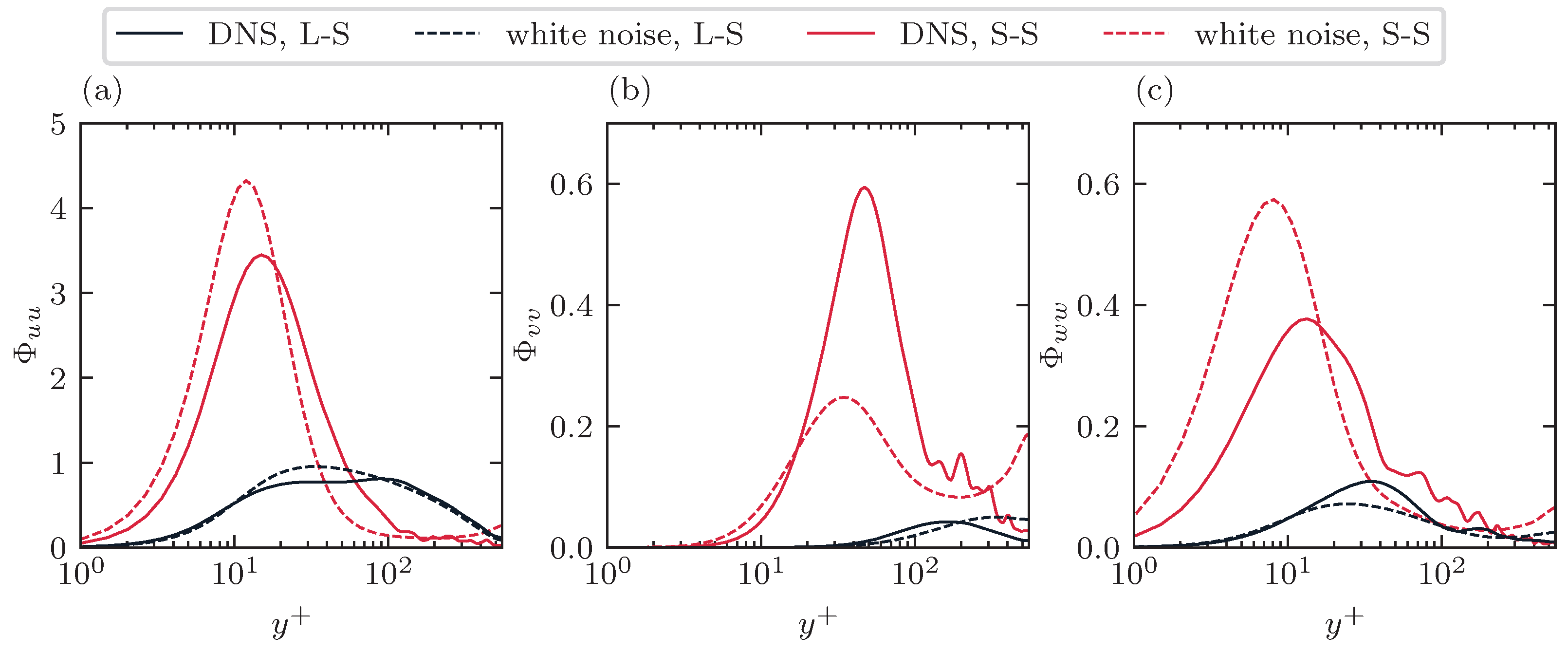
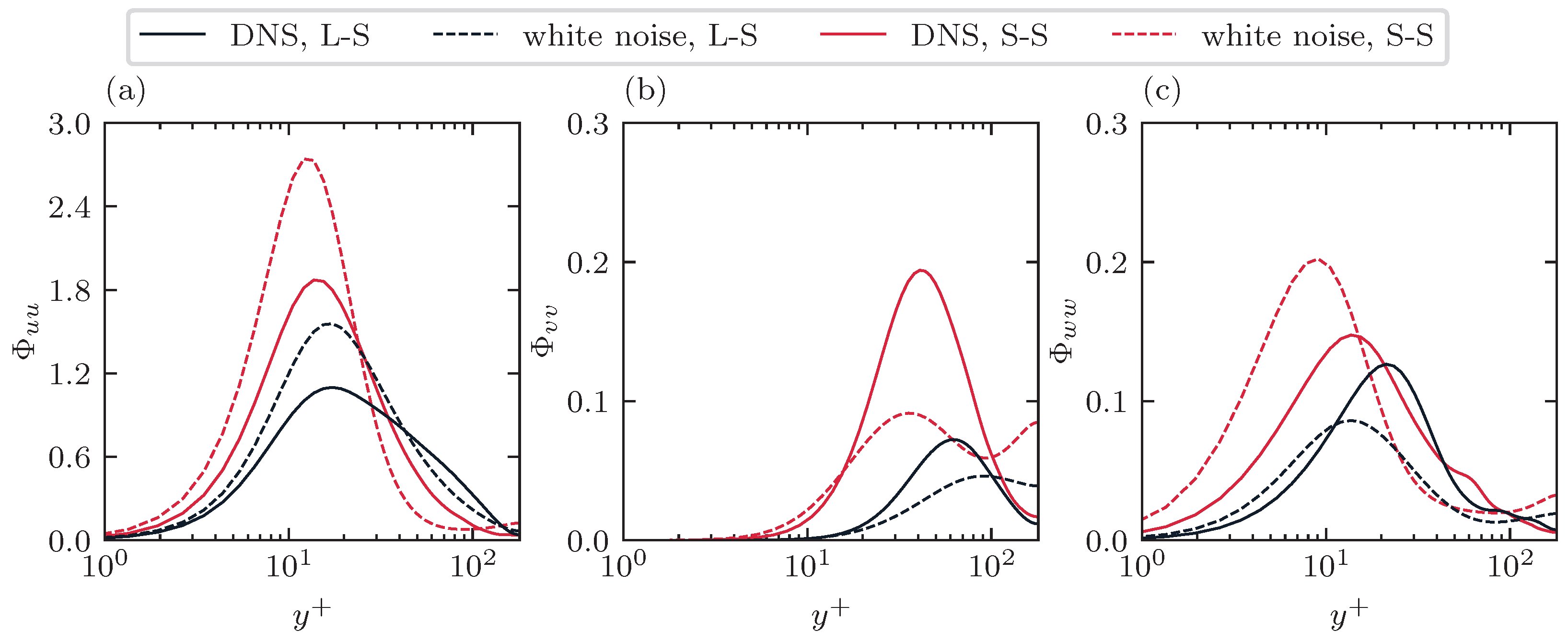
Figure 2 and Figure 3 show the wall-normal distributions of the power spectral density (PSD) of the three velocity components for large and small scales at friction Reynolds numbers $R{e}_{\tau }=180$ and 550, respectively. For both Reynolds numbers, substantial discrepancies between the resolvent predictions and the DNS data are observed. First, the streamwise and spanwise velocity components exhibit overpredicted peaks, whereas the wall-normal component is underpredicted relative to DNS. Second, for all three components, the resolvent model predicts excessive spectral energy in the channel center, with particularly pronounced deviations for the wall-normal and spanwise velocities. As a consequence, the resolvent spectra display three distinct peaks: one at the channel center and two near the critical layers. In contrast, the DNS results show only two peaks located near the critical layers.

These discrepancies originate from the assumption of wall-normal uniform white-in-time forcing. Such forcing injects excessive energy throughout the domain, particularly away from the critical layers, leading to wall-normal energy distributions that differ markedly from those observed in DNS.

Next, we examine the conditional frequency spectra, defined as

$${\Phi }_{ii}={\displaystyle \frac{\langle {\tilde{u}}_i{\tilde{u}}_i^{\ast }\rangle }{{\sum }_{j=1}^3{\int }_{-\infty }^{\infty }{\int }_{-h}^h\langle {\tilde{u}}_j{\tilde{u}}_j^{\ast }\rangle \mathrm{d}y \mathrm{d}\omega }}.$$

(19)

This normalization highlights the relative distribution of energy across wall-normal position and frequency, as well as among the three velocity components.

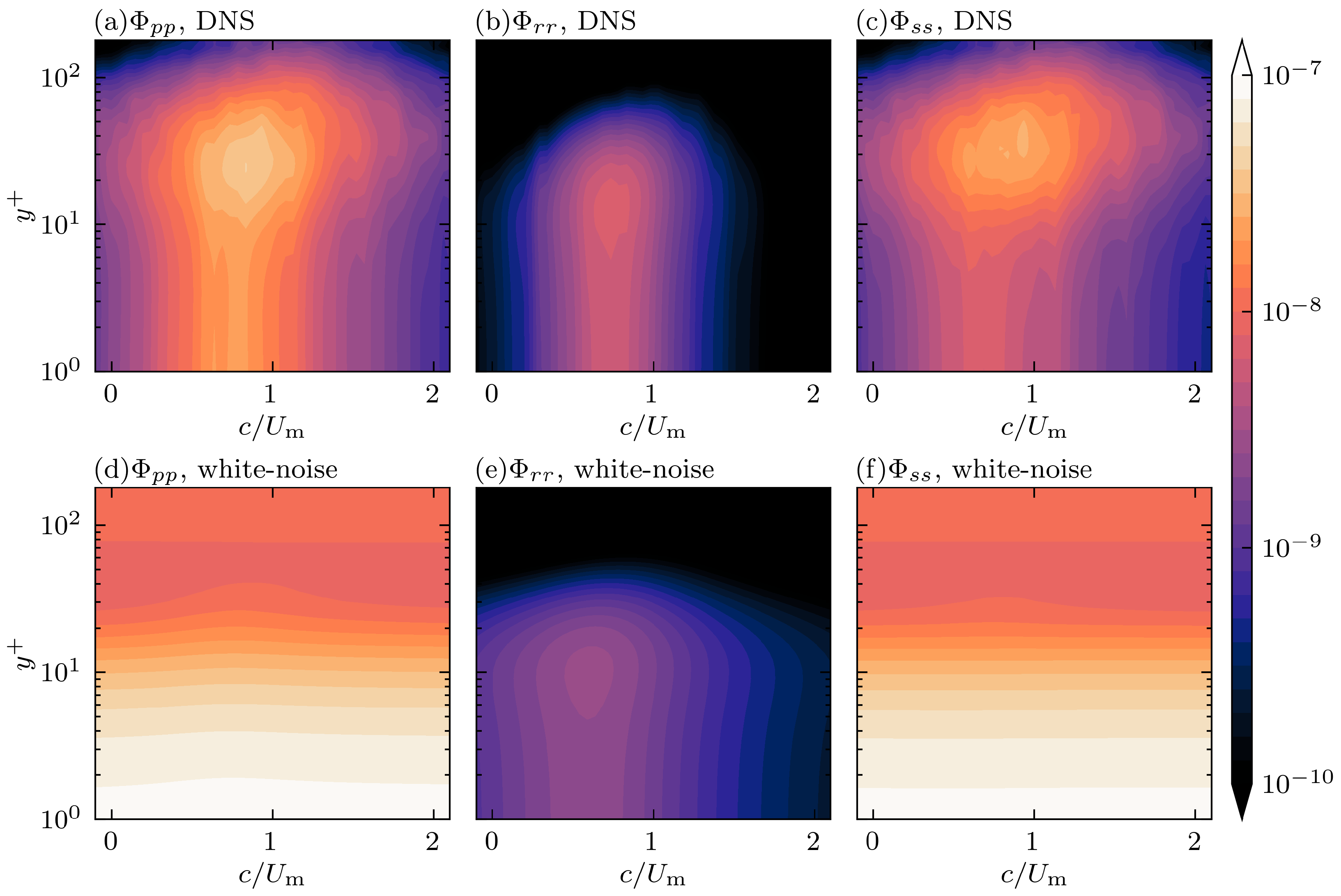
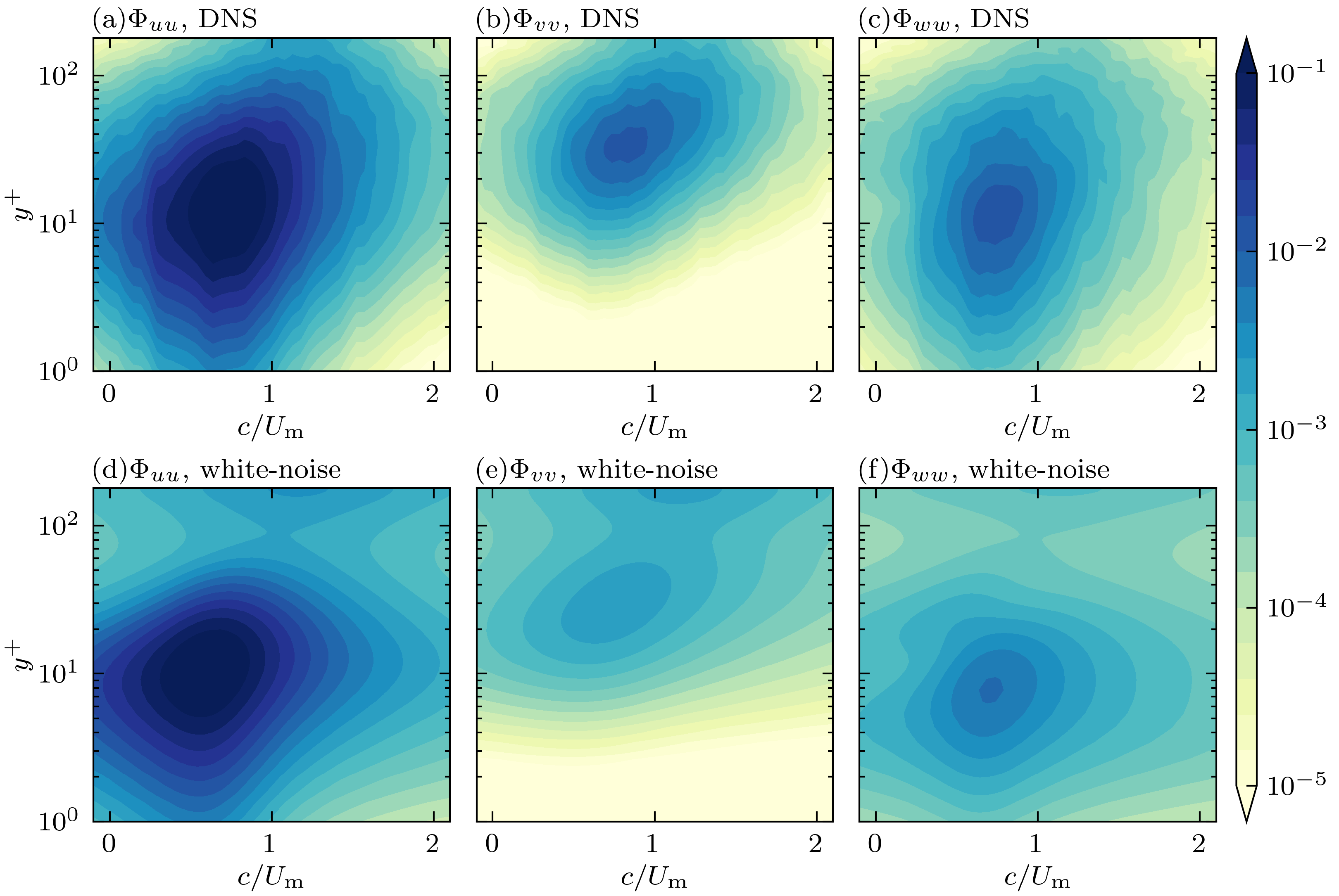
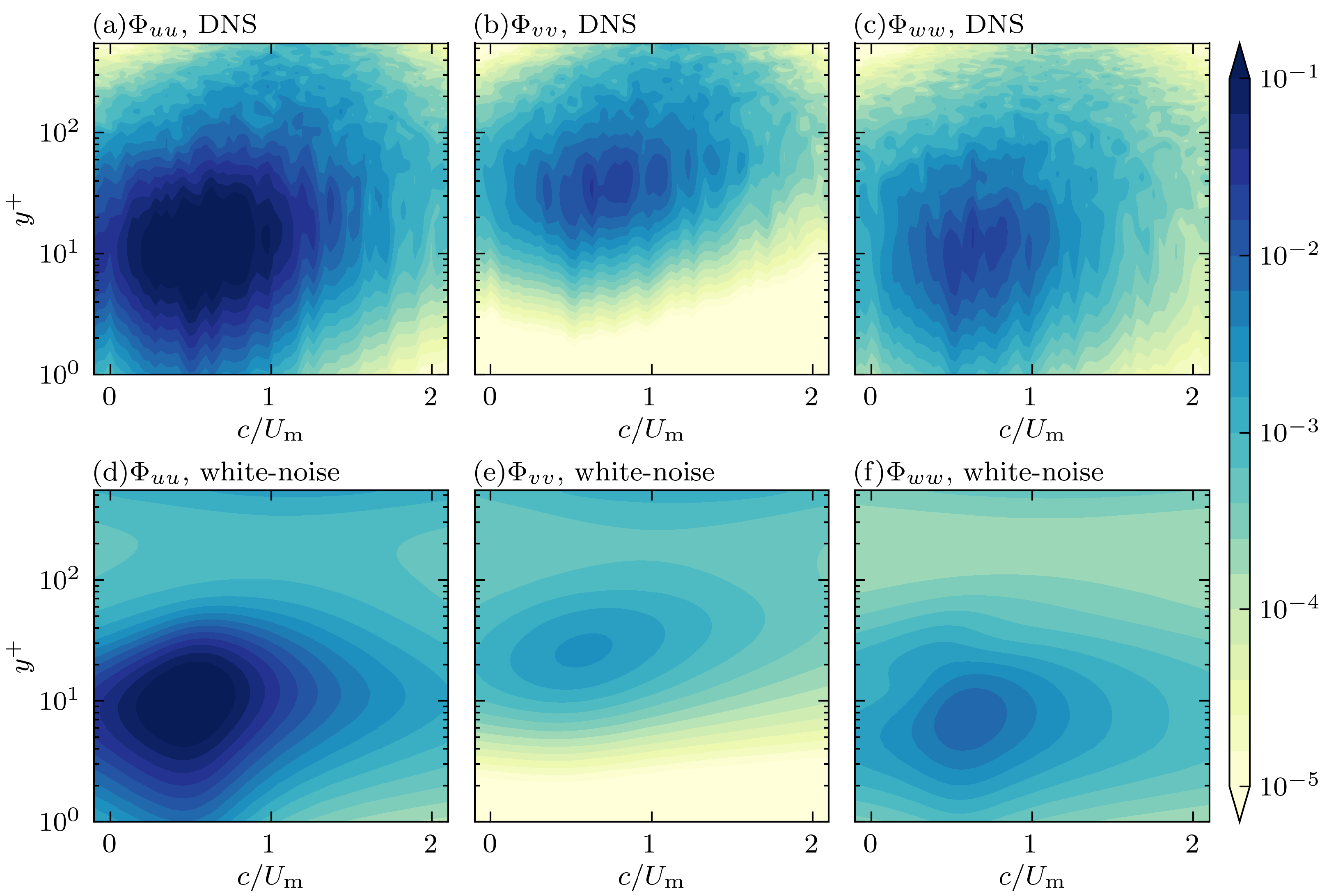
Figure 4 and Figure 5 present the conditional frequency spectra for the small scale for $R{e}_{\tau }=180$ and 550, respectively. In each subplot, the horizontal axis represents the wavespeed, defined as the wavenumber-normalized frequency $c=\omega /k_x$, while the vertical axis denotes the wall-normal distance measured in viscous units, $y^{+}$. At the streak scale, the streamwise wavelength is much larger than the spanwise wavelength, and the streamwise velocity component carries the largest fraction of energy at all frequencies. The resolvent predictions successfully reproduce the relative ordering of energy among the three velocity components. However, at each wall-normal location, the resolvent model predicts a substantially broader frequency distribution for a given energy level. This behavior is evident from the markedly flatter isocontours in the resolvent predictions compared with the DNS results. The three wall-normal peaks predicted by the resolvent analysis, as shown in Figure 2 and Figure 3, are also clearly manifested in the frequency–wall-normal spectra. In particular, the concave shape of the resolvent isocontours implies that a vertical line corresponding to a fixed frequency intersects a given contour level up to six times between the lower and upper walls, reflecting the presence of three distinct wall-normal energy maxima.

To quantitatively assess the accuracy of the frequency-spectrum predictions, we examine the convection velocity of each velocity component, defined following [27] as,

$$c_i=-{\displaystyle \frac{1}{k_x}}{\displaystyle \frac{{\int }_{-\infty }^{\infty }\omega \langle {\tilde{u}}_i{\tilde{u}}_i^{\ast }\rangle \mathrm{d}\omega }{{\int }_{-\infty }^{\infty }\langle {\tilde{u}}_i{\tilde{u}}_i^{\ast }\rangle \mathrm{d}\omega }}.$$

(20)

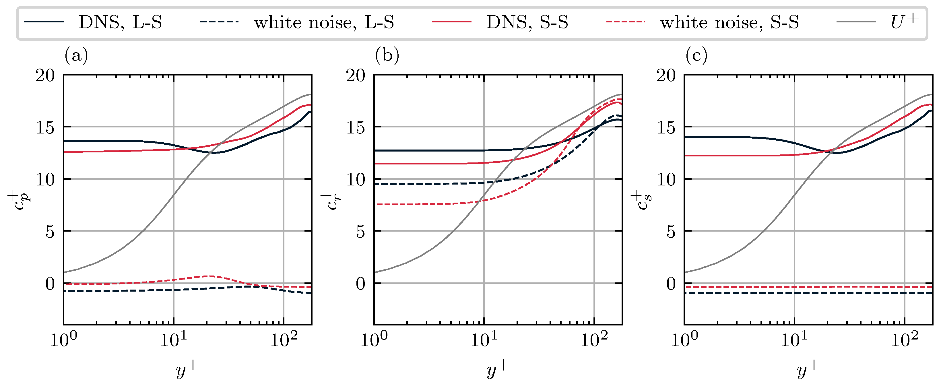
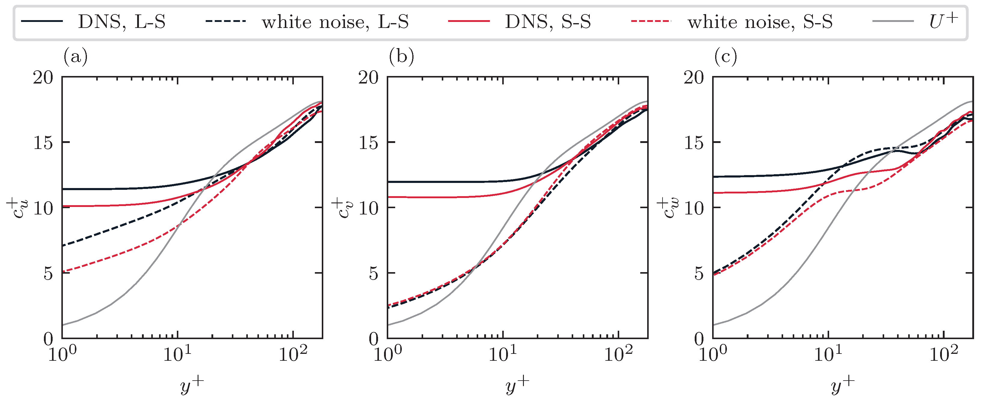
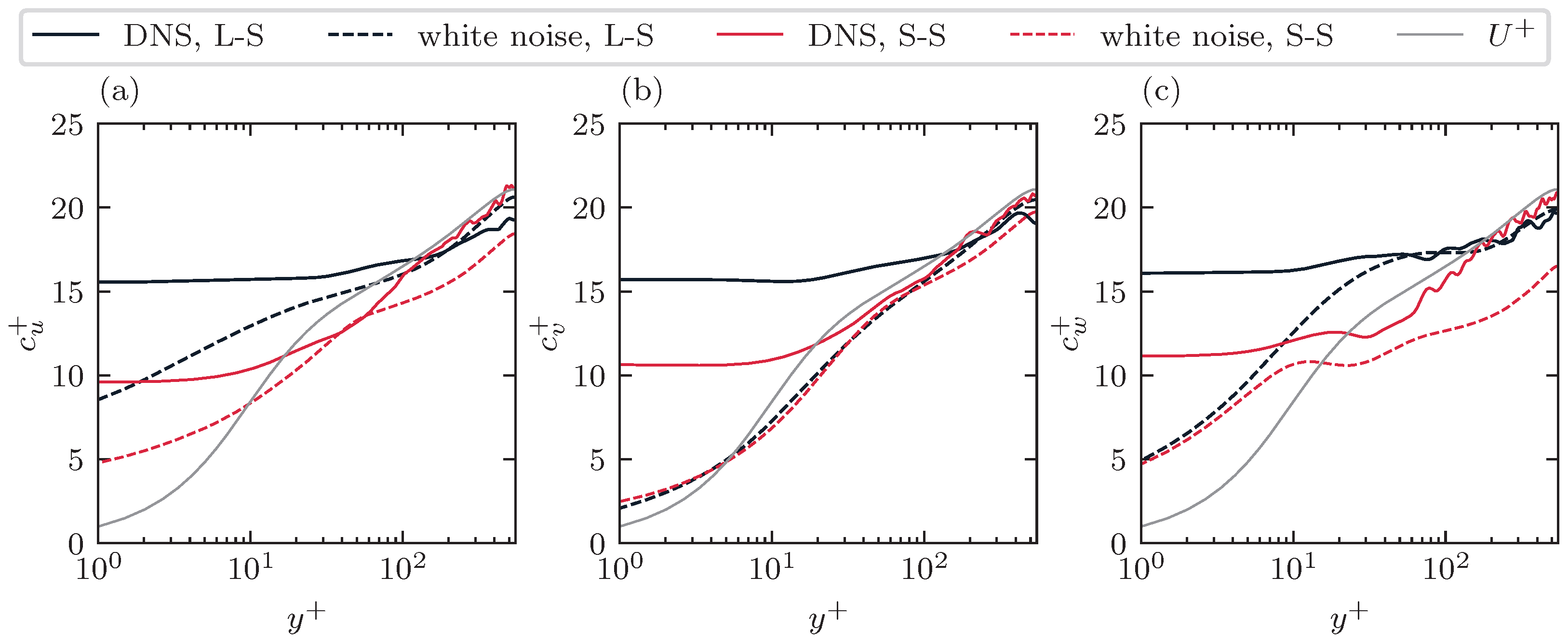
The convection velocity defined above represents the average phase velocity of each scale. It is interpreted as the value that minimizes the discrepancy between the actual temporal evolution of $u_i$ and a frozen wave propagating as $u_i(x-c_{i}t)$. Figure 6 and Figure 7 present the convection velocities of the three velocity components for the large and small scales predicted by resolvent analysis, together with DNS results and the mean velocity profile, for $R{e}_{\tau }=180$ and 550 respectively. The DNS results show that the convection velocity is approximately constant within the viscous sublayer and buffer layer, with a value of $c^{+}=10$, and remains slightly below the local mean velocity in the logarithmic layer. In contrast, the resolvent predictions exhibit substantial discrepancies relative to DNS. In the viscous sublayer and buffer layer, the predicted convection velocities are significantly smaller than the DNS values and do not display a plateau. In the logarithmic region, the resolvent predictions are reasonably close to DNS at $R{e}_{\tau }=180$, but substantially underpredict the convection velocity at $R{e}_{\tau }=550$. Since the convection velocity represents the first moment of the frequency spectrum, these discrepancies indicate that the most energetic frequencies are systematically mispredicted when white-in-time forcing is assumed. To further characterize the distribution of energy in frequency space, we compute the Taylor time microscale, defined as

$${\lambda }_T={\left(-{\displaystyle \frac{1}{2}}{\displaystyle \frac{{\mathsf{\partial }}^2\left|R\right|}{\mathsf{\partial }{\tau }^2}}{|}_{\tau =0}\right)}^{-1/2},$$

(21)

where the temporal separation is denoted by $\tau$ and $\left|R\right|$ is the magnitude of the temporal autocorrelation function. The correlation function is calculated from the frequency spectrum as

$$R(\mathit{k},\tau ,y)={\displaystyle \frac{{\int }_{-\infty }^{\infty }\langle \tilde{\varphi }{\tilde{\varphi }}^{\ast }\rangle e^{\mathrm{i}\omega \tau }\mathrm{d}\omega }{{\int }_{-\infty }^{\infty }\langle \tilde{\varphi }{\tilde{\varphi }}^{\ast }\rangle \mathrm{d}\omega }},$$

(22)

where $\varphi$ denotes an arbitrary flow variable. From the definition (21), the Taylor time microscale can be expressed in terms of the spectral bandwidth as

$${\lambda }_T=\sqrt{{\displaystyle \frac{2}{B}}},$$

(23)

where the bandwidth B of the frequency spectrum is defined by

$$B={\int }_{-\infty }^{\infty }{\left(\omega -{\omega }_c\right)}^2\Phi \mathrm{d}\omega ,\Phi ={\displaystyle \frac{\langle \tilde{\varphi }{\tilde{\varphi }}^{\ast }\rangle }{{\int }_{-\infty }^{\infty }\langle \tilde{\varphi }{\tilde{\varphi }}^{\ast }\rangle \mathrm{d}\omega }},{\omega }_c={\int }_{-\infty }^{\infty }\omega \Phi \mathrm{d}\omega .$$

(24)

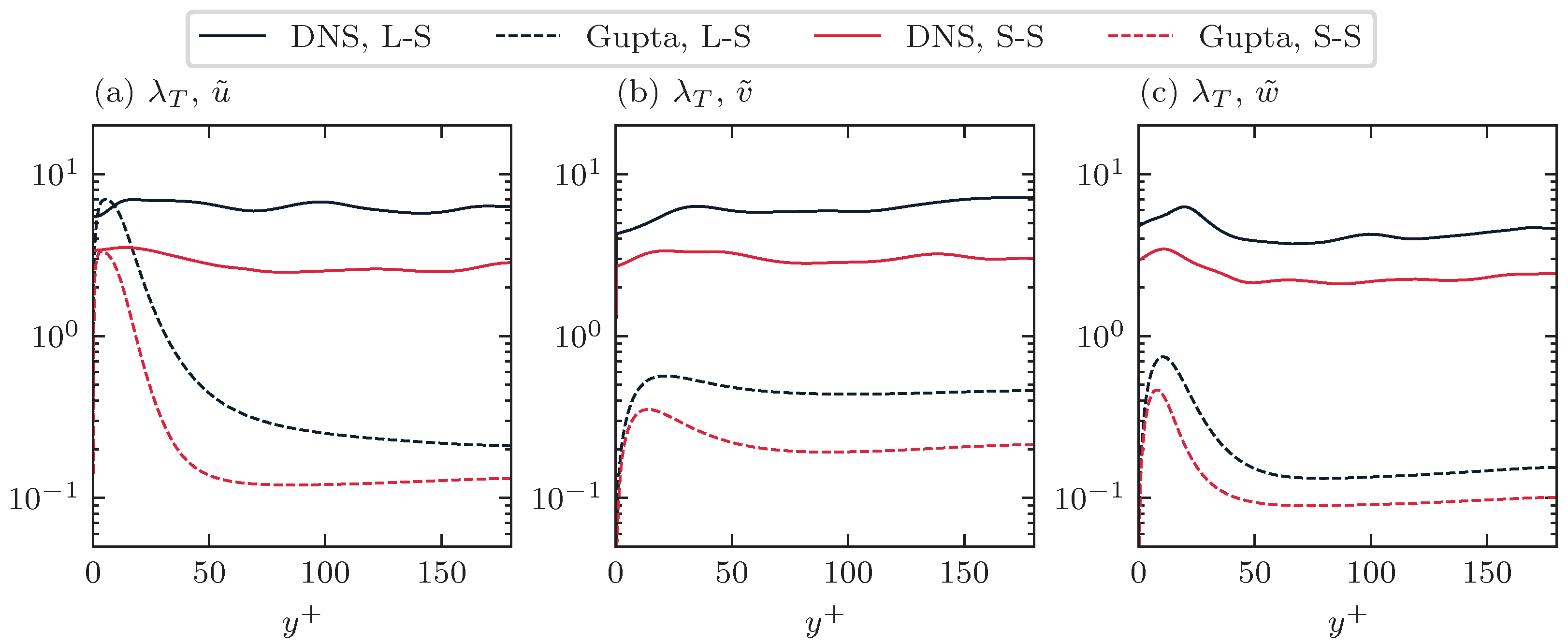
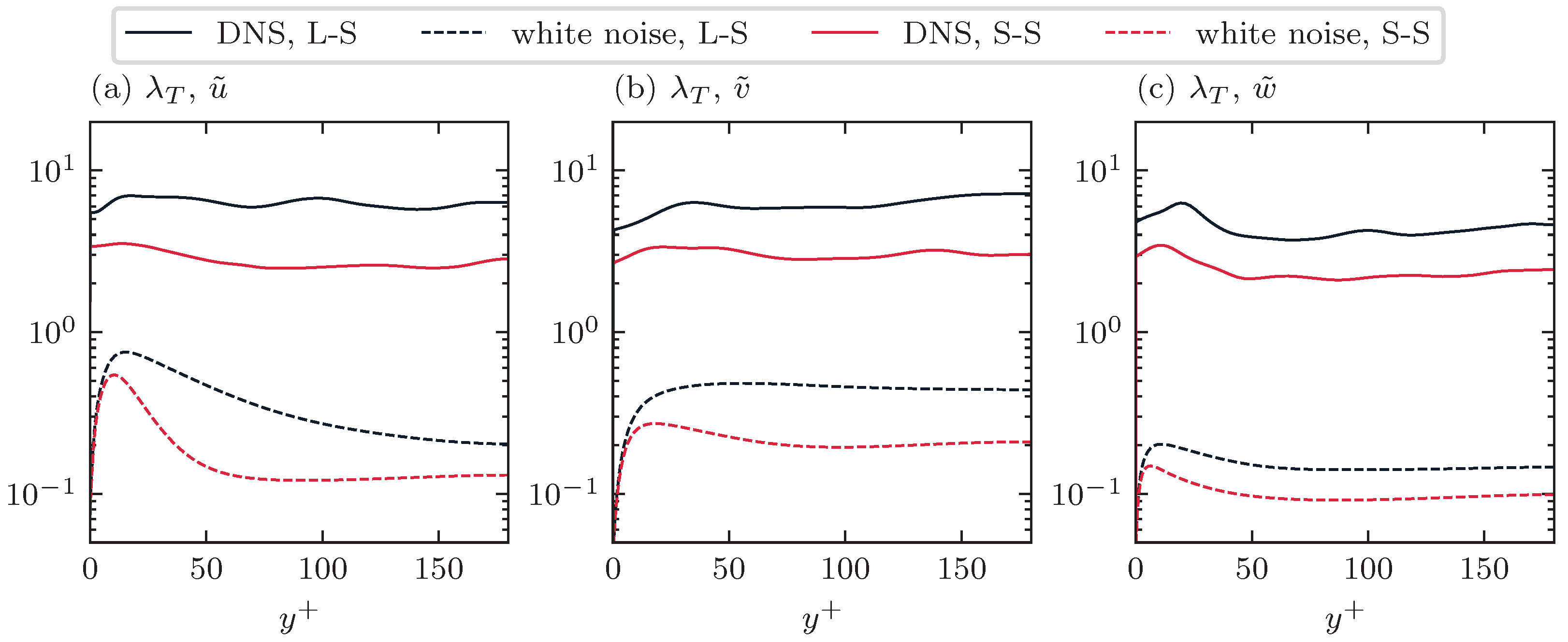
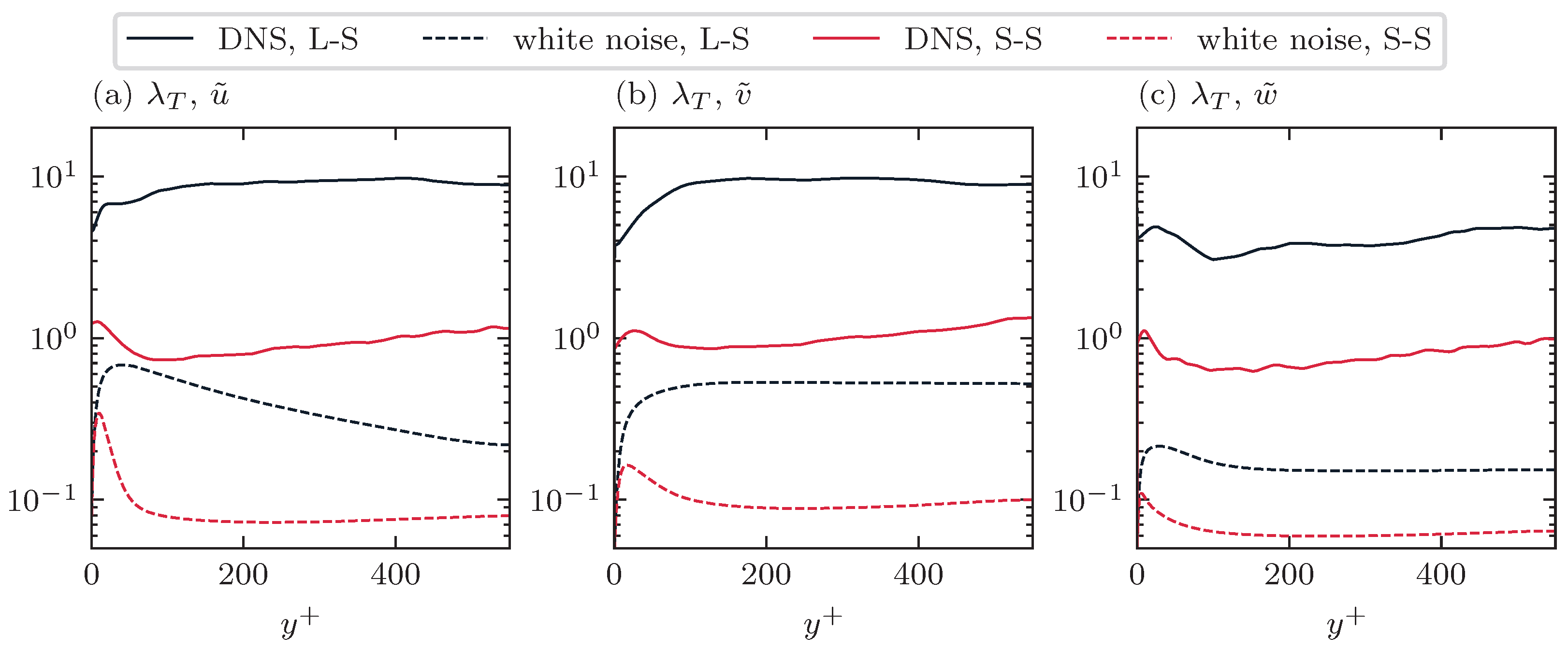
In Figure 8 ($R{e}_{\tau }=180$) and Figure 9 ($R{e}_{\tau }=550$), we present the Taylor time microscales associated with the three velocity components. It is evident that the Taylor time microscales predicted by the resolvent analysis with white-in-time stochastic forcing are significantly smaller than those obtained from DNS. This severe underprediction represents the principal deficiency of the white-in-time forcing assumption and constitutes the primary limitation emphasized in the present study. The poor performance in predicting the Taylor time microscale can be understood through a simplified linear convection–diffusion model,

$${\displaystyle \frac{\mathsf{\partial }\varphi }{\mathsf{\partial }t}}+c{\displaystyle \frac{\mathsf{\partial }\varphi }{\mathsf{\partial }x}}=\kappa {\displaystyle \frac{{\mathsf{\partial }}^2\varphi }{\mathsf{\partial }{x}^2}}+\sigma ,$$

(25)

where $\varphi$ denotes the convected variable, c is the convection velocity, $\kappa$ is a constant diffusion coefficient, and $\sigma$ represents a white-in-time stochastic forcing. Taking the space–time Fourier transform of (25) yields

$$\left(-\mathrm{i}\omega +\mathrm{i}{k}_{x}c+\kappa k_x^2\right)\tilde{\varphi }=\tilde{\sigma }.$$

(26)

Assuming $\langle \tilde{\sigma }{\tilde{\sigma }}^{\ast }\rangle =1$, the conditional frequency spectrum and the corresponding central frequency ${\omega }_c$ are given by

$${\Phi }_{\varphi \varphi }={\displaystyle \frac{\kappa k_x^2}{\pi }}{\displaystyle \frac{1}{{\kappa }^2{k}_x^4+{\left(\omega -k_{x}c\right)}^2}},$$

(27)

However, the second moment of this spectrum,

$${\int }_{-\infty }^{\infty }{\displaystyle \frac{\kappa k_x^2}{\pi }}{\displaystyle \frac{{\omega }^2}{{\kappa }^2{k}_x^4+{\left(\omega -k_{x}c\right)}^2}}\mathrm{d}\omega \to \infty$$

(28)

diverges, implying an infinite spectral bandwidth and, consequently, a vanishing Taylor time microscale.

This behavior arises because white-in-time stochastic forcing injects energy uniformly across all frequencies, resulting in an unphysically broad frequency spectrum. As a consequence, such forcing cannot represent a physically meaningful temporal decorrelation process. This deficiency is critical, as realistic time decorrelation is essential for accurately modeling and predicting turbulence statistics in the temporal dimension.

Figure 6. The convection velocity of (a) streamwise, (b) wall-normal, and (c) spanwise velocity. Predictions from resolvent analysis with white-in-time stochastic forcing (dashed lines) are compared with DNS results (solid lines). Results are shown for large scale ${\lambda }_x=4\pi$, ${\lambda }_z=0.4\pi$ (black) and small scale ${\lambda }_x^{+}=1000$, ${\lambda }_z^{+}=100$ (red), $R{e}_{\tau }=180$.

Figure 6. The convection velocity of (a) streamwise, (b) wall-normal, and (c) spanwise velocity. Predictions from resolvent analysis with white-in-time stochastic forcing (dashed lines) are compared with DNS results (solid lines). Results are shown for large scale ${\lambda }_x=4\pi$, ${\lambda }_z=0.4\pi$ (black) and small scale ${\lambda }_x^{+}=1000$, ${\lambda }_z^{+}=100$ (red), $R{e}_{\tau }=180$.

Figure 7. (a) The same as Figure 6a but for $R{e}_{\tau }=550$; (b) The same as Figure 6b but for $R{e}_{\tau }=550$; (c) The same as Figure 6c but for $R{e}_{\tau }=550$.

Figure 7. (a) The same as Figure 6a but for $R{e}_{\tau }=550$; (b) The same as Figure 6b but for $R{e}_{\tau }=550$; (c) The same as Figure 6c but for $R{e}_{\tau }=550$.

Figure 8. The Taylor time microscales of (a) streamwise, (b) wall-normal, and (c) spanwise velocity. Predictions from resolvent analysis with white-in-time stochastic forcing (dashed lines) are compared with DNS results (solid lines). Results are shown for large scale ${\lambda }_x=4\pi$, ${\lambda }_z=0.4\pi$ (black) and small scale ${\lambda }_x^{+}=1000$, ${\lambda }_z^{+}=100$ (red), $R{e}_{\tau }=180$.

Figure 8. The Taylor time microscales of (a) streamwise, (b) wall-normal, and (c) spanwise velocity. Predictions from resolvent analysis with white-in-time stochastic forcing (dashed lines) are compared with DNS results (solid lines). Results are shown for large scale ${\lambda }_x=4\pi$, ${\lambda }_z=0.4\pi$ (black) and small scale ${\lambda }_x^{+}=1000$, ${\lambda }_z^{+}=100$ (red), $R{e}_{\tau }=180$.

Figure 9. (a) The same as Figure 8a but for $R{e}_{\tau }=550$; (b) The same as Figure 8b but for $R{e}_{\tau }=550$; (c) The same as Figure 8c but for $R{e}_{\tau }=550$.

Figure 9. (a) The same as Figure 8a but for $R{e}_{\tau }=550$; (b) The same as Figure 8b but for $R{e}_{\tau }=550$; (c) The same as Figure 8c but for $R{e}_{\tau }=550$.

3.2. Pressure Prediction

The previous section systematically investigated the frequency spectra prediction of the velocity components. In this section, we provide a detailed assessment of the resolvent prediction for the pressure spectra and its decomposition into rapid and slow components.

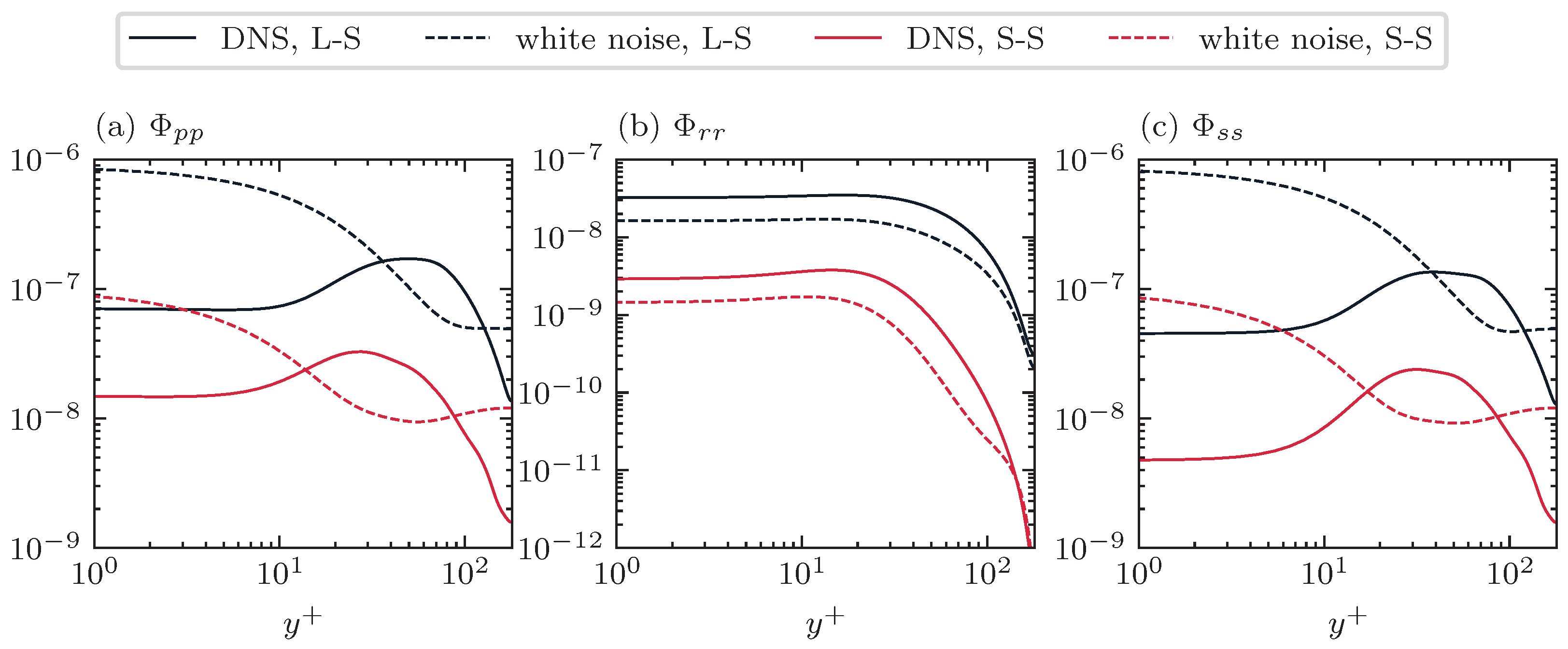
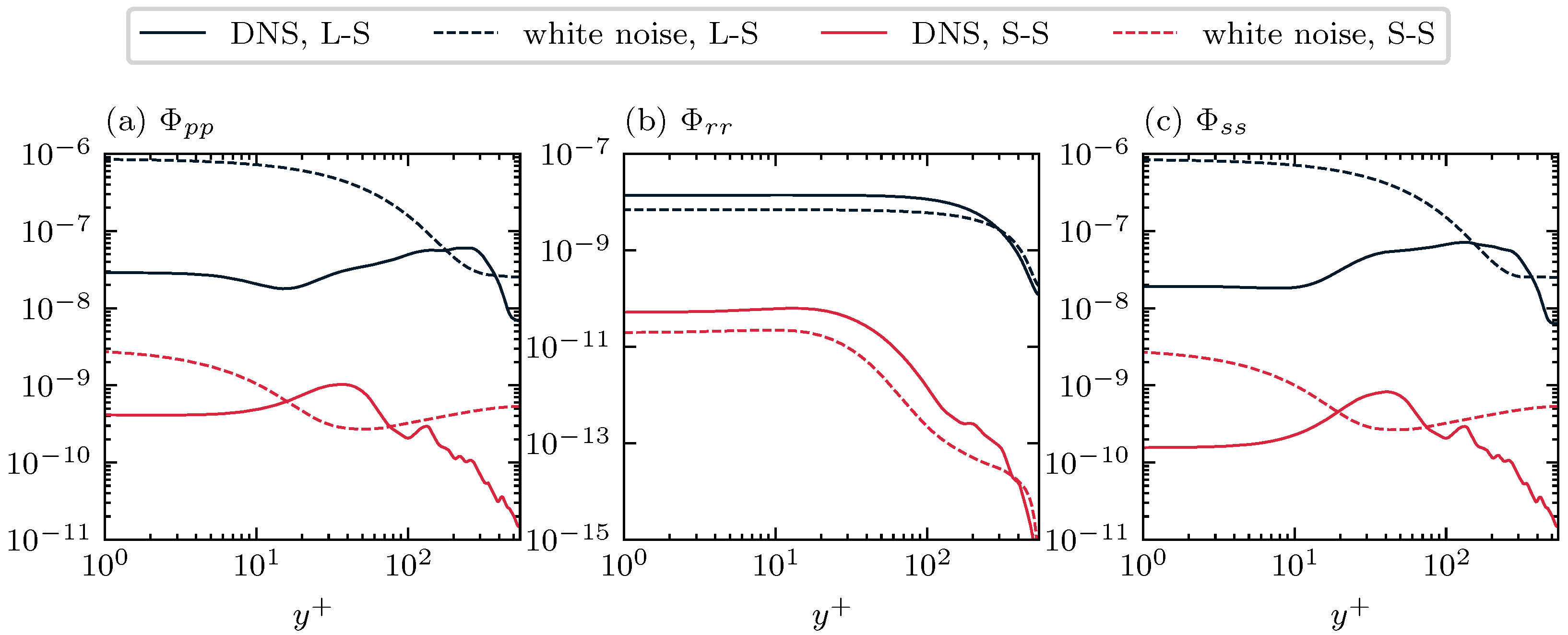
First, the PSDs of the pressure, as well as those of the rapid and slow pressure components at $c/U_m=1$, are shown in Figure 10 and Figure 11 for $R{e}_{\tau }=180$ and 550, respectively. The intensity of the white-noise stochastic forcing is determined by matching the wall-integrated kinetic energy with that of the DNS data, allowing a direct comparison of the predicted pressure PSDs with DNS results.

From Figure 10 and Figure 11, it is evident that the resolvent predictions fail to capture the pressure statistics accurately. For the total pressure PSD, the resolvent model does not reproduce the two peaks observed in DNS and instead predicts excessively large values near the walls, which decay rapidly away from the wall. For the rapid pressure PSD, although the two peaks are qualitatively captured, the predicted intensity is significantly lower than the DNS. The slow pressure PSD behaves similarly to the total pressure, with neither peak being reproduced and with substantially overpredicted wall values. These discrepancies become even more pronounced at the higher Reynolds number ${\Re }_{\tau }=550$. In particular, the resolvent predictions for the pressure and slow pressure are markedly overestimated near the wall and in the inertial region, whereas they are underpredicted in regions where the DNS exhibits strong pressure fluctuations.

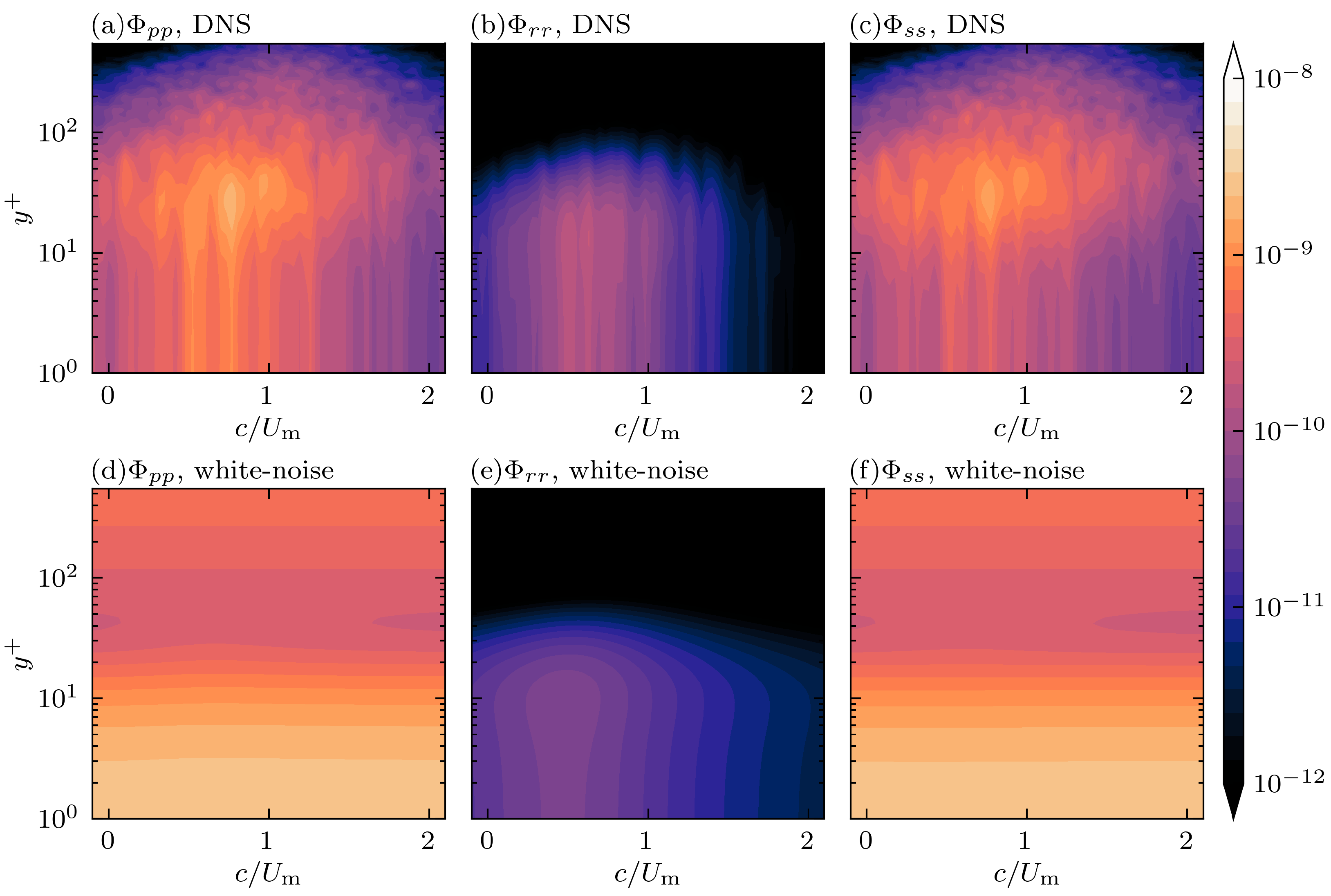
The frequency–wall-normal distributions of the pressure, rapid pressure, and slow pressure spectra are presented in Figure 12 and Figure 13 of the small scales for $R{e}_{\tau }=180$ and 550, respectively. In each figure, the resolvent predictions are compared with DNS results. For both the total pressure and the slow pressure, the resolvent model fails to capture the correct wall-normal locations of the spectral peaks and does not reproduce the observed decay of energy as the frequency departs from $c/U_m=1$. This behavior is particularly evident in Figure 12 and Figure 13d,f, where the isolines remain nearly horizontal, indicating little variation in peak position with frequency.

For the rapid pressure component, the resolvent prediction yields a substantially lower intensity and a noticeably broader frequency bandwidth compared with DNS.

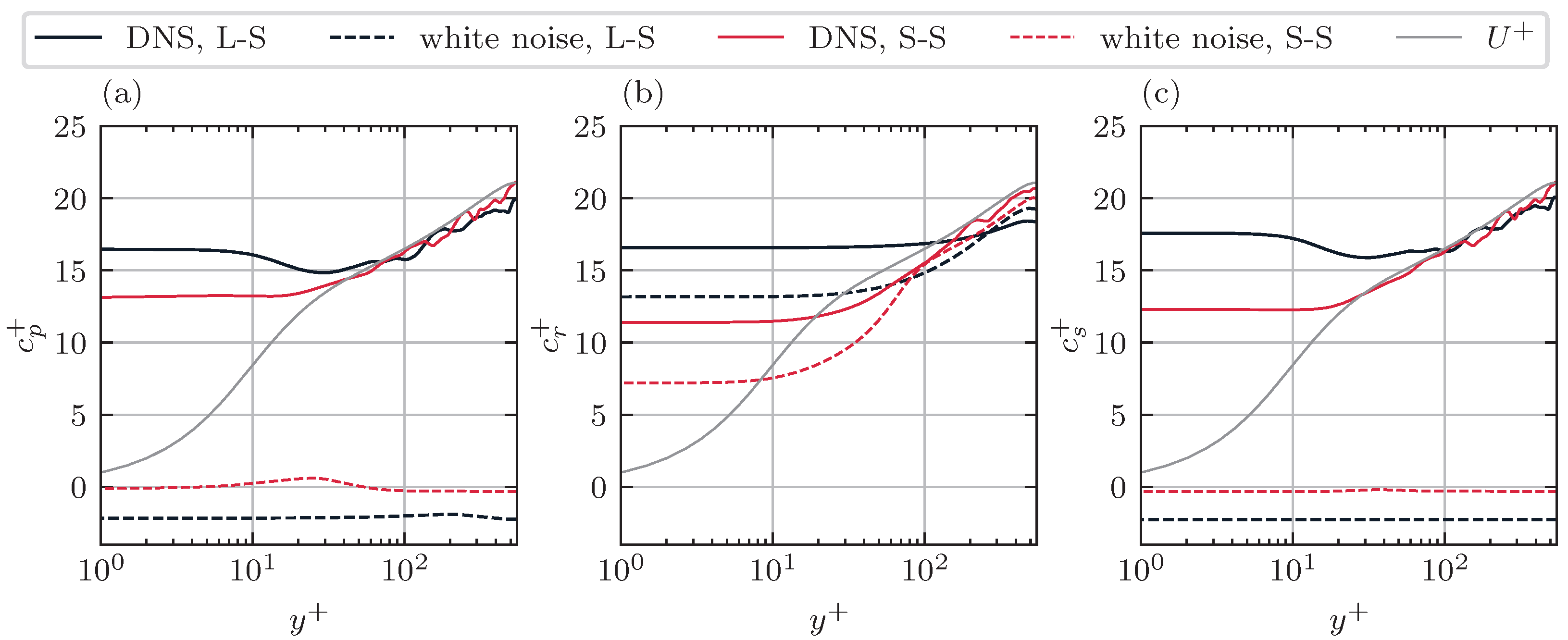
The convection velocities for the total pressure, rapid pressure, and slow pressure are shown in Figure 14 and Figure 15 of both large and small scales for $R{e}_{\tau }=180$ and 550, respectively. For both Reynolds numbers, the convection velocities are nearly constant within the viscous layer, with values around $c^{+}=12$, slightly larger than the convection velocity of the velocity fluctuations at the same scale. In the inertial region, the convection velocity is somewhat smaller than the mean velocity for $R{e}_{\tau }=180$ and nearly identical to the mean velocity for $R{e}_{\tau }=550$.

However, among the three pressure components, only the rapid pressure in the inertial region shows a partial agreement between resolvent predictions and DNS results. In the viscous layer, although the resolvent model predicts an approximately constant convection velocity, its magnitude is significantly lower than that observed in DNS. For the total pressure and slow pressure, the resolvent predictions yield convection velocities that are close to zero or even negative across much of the channel height.

These substantial discrepancies demonstrate that white-in-time stochastic forcing is unable to capture the correct temporal dynamics of pressure fluctuations, which explains its poor performance in predicting pressure statistics.

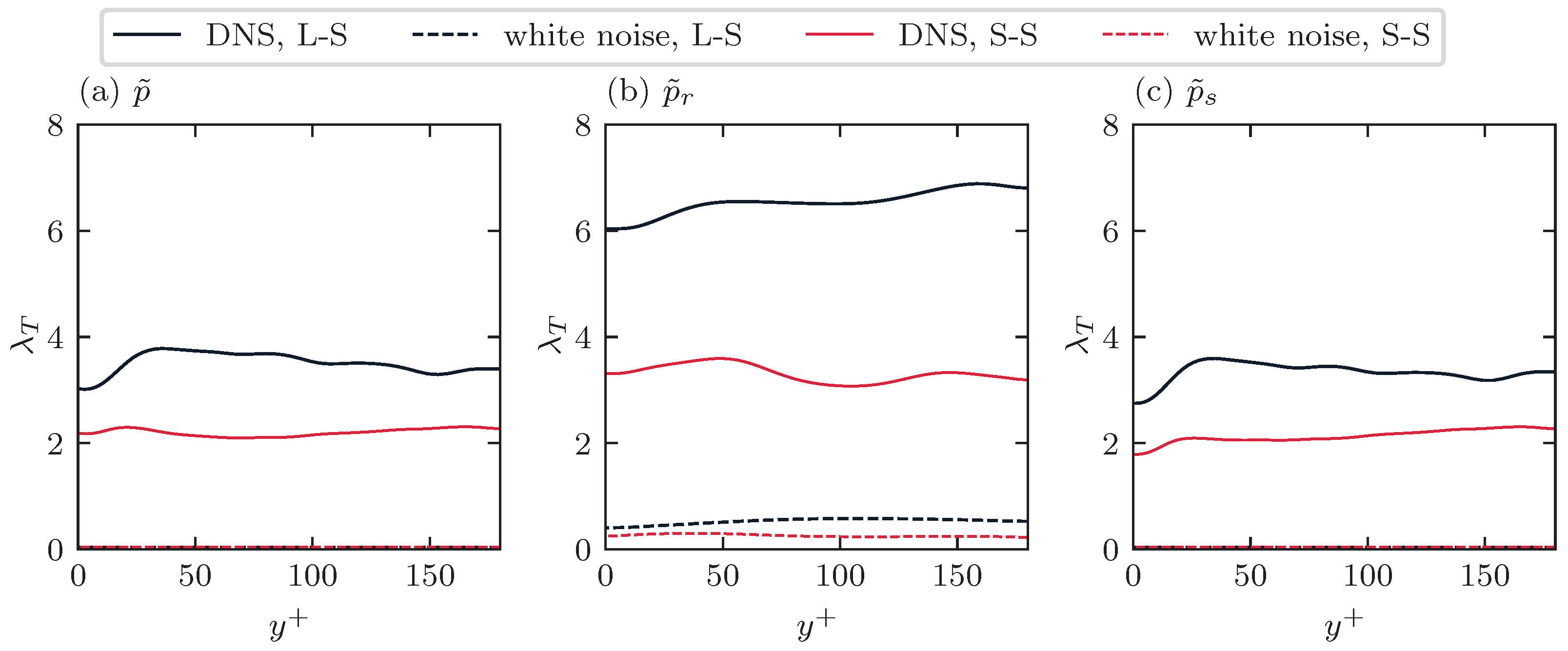
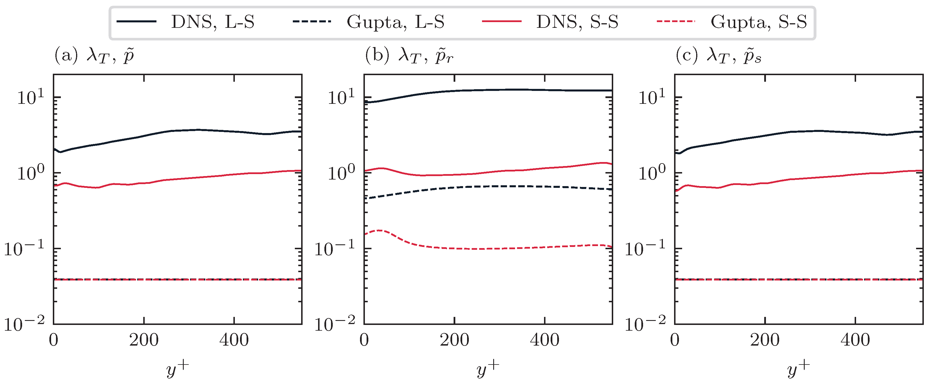
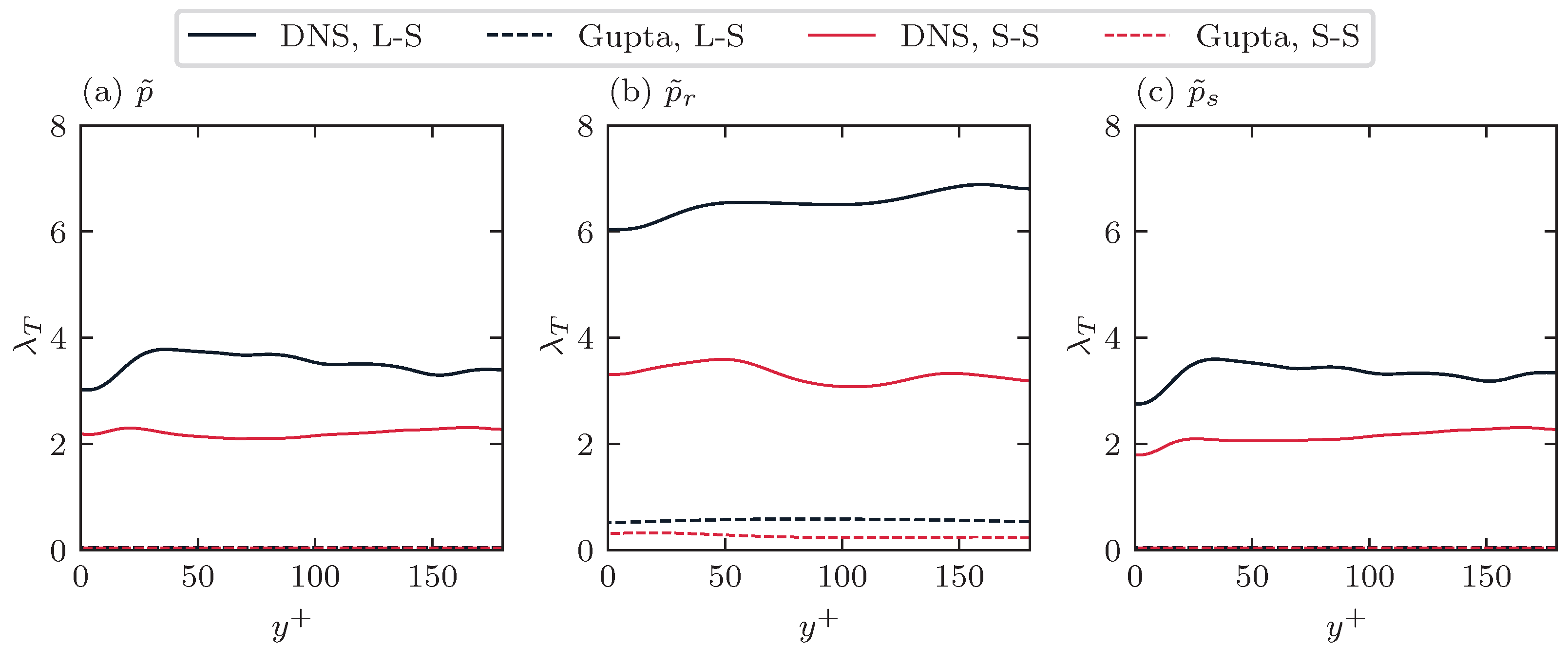
To quantify the prediction of frequency spectra, the Taylor time scales of the pressure components are further examined in Figure 16 and Figure 17 for $R{e}_{\tau }=180$ and 550, respectively. For both Reynolds numbers, the DNS results show that the Taylor time scales of the total pressure and the slow pressure are nearly identical at this scale, while the rapid pressure exhibits a larger Taylor time microscale than the other two components.

In contrast, the Taylor time scales predicted by the resolvent model with white-in-time stochastic forcing are nearly zero for all pressure components. This finding further confirms the ineffectiveness of white-in-time forcing in capturing the temporal structure of pressure fluctuations.

In the preceding sections, the PSDs of the total pressure and its rapid and slow components were examined in detail. The following analysis focuses on understanding the underlying reasons for the discrepancies observed in the pressure PSD predictions.

The rapid pressure PSD can be obtained directly from the Poisson equation as

$$\langle {\tilde{p}}_r{\tilde{p}}_r^{\ast }\rangle =4k_x^2{\Delta }^{-1}{U}^{\prime }\langle \tilde{v}{\tilde{v}}^H\rangle U^{\prime T}{\Delta }^{-H},$$

(29)

where ${\Delta }^{-H}={\left({\Delta }^{-1}\right)}^H$, and $U^{\prime T}$ denotes the transpose of $U^{\prime }$. This expression indicates that the rapid pressure PSD is determined solely by the cross-spectral density of the wall-normal velocity.

Therefore, the underprediction of the rapid pressure PSD directly reflects a deficit in the predicted wall-normal velocity CSD. Since the wall-normal velocity statistics are obtained through the resolvent input–output relationship driven by white-in-time forcing, this deficiency implies that white-in-time forcing is incapable of reproducing the correct two-point correlations of the velocity field. A detailed discussion of the failure of white-noise forcing in reproducing two-point correlations is provided by Zare et al. [11], and readers are referred to that work for a more rigorous explanation.

It is worth noting that, although the white-in-time forcing is explicitly modeled as spatially decorrelated in the wall-normal direction, the solenoidal projection of the forcing inevitably introduces wall-normal two-point correlations. As rigorously proved by Holford et al. [12], a forcing field that is decorrelated in space cannot be solenoidal; thus, the solenoidal component of white-in-time forcing must contain spatial correlation. However, the presence of such correlation is still insufficient to recover the correct velocity correlations.

From the Poisson equation, the slow pressure PSD can be expressed as

$$\begin{array}{cc}\hfill \langle {\tilde{p}}_s{\tilde{p}}_s^{\ast }\rangle =& 2H\left[2{\Delta }^{-1}({\nu }_t^{\prime }\Delta +{\nu }_t^{″}\mathcal{D})\langle \tilde{v}{\tilde{\varrho }}^H\rangle {\Delta }^{-H}\right]\hfill \\ & +4{\Delta }^{-1}\left({\nu }_t^{\prime }\Delta +{\nu }_t^{″}\mathcal{D}\right)\langle \tilde{v}{\tilde{v}}^H\rangle {\left({\nu }_t^{\prime }\Delta +{\nu }_t^{″}\mathcal{D}\right)}^H{\Delta }^{-H}\hfill \\ & +{\Delta }^{-1}\langle \tilde{\varrho }{\tilde{\varrho }}^H\rangle {\Delta }^{-H},\hfill \end{array}$$

(30)

which indicates that the slow pressure PSD originates from three distinct sources: (i) the two-point correlation between the wall-normal velocity and the forcing divergence, $\langle \tilde{v}{\tilde{\varrho }}^H\rangle$; (ii) the two-point correlation of the wall-normal velocity, $\langle \tilde{v}{\tilde{v}}^H\rangle$; and (iii) the two-point correlation of the stochastic forcing divergence, $\langle \tilde{\varrho }{\tilde{\varrho }}^H\rangle$.

The pronounced burst of the slow pressure PSD near the wall suggests that the divergence of the stochastic forcing is excessively large in that region. This behavior implies that a wall-normal uniform white-in-time forcing cannot provide a physically consistent two-point correlation of the nonlinear forcing divergence. Moreover, since a similar near-wall burst is observed in both the total pressure and the slow pressure PSD, the correlation between the rapid and slow pressure components is likely not the dominant contribution to the pressure PSD discrepancy.

A more detailed decomposition of the slow pressure PSD, including the relative contributions of each term, is not pursued here and remains a topic for future work.

4. Conclusions

In this study, we systematically assessed the performance of the eddy-viscosity-enhanced resolvent framework driven by white-in-time stochastic forcing for predicting velocity and pressure frequency spectra in turbulent channel flow. The key finding of this work is that the white-in-time stochastic forcing assumption introduces fundamental deficiencies in the temporal statistics of both velocity and pressure fields. By injecting energy uniformly across all frequencies, the white-in-time forcing produces excessively broad frequency spectra, leading to vanishing Taylor time microscales for both velocity and pressure components. The failure is not limited to the velocity field; it propagates to pressure statistics, where the resolvent model predicts unphysically strong pressure fluctuations near the walls and fails to reproduce the correct wall-normal distribution and spectral decay with frequency. The pressure decomposition further highlights that both the rapid and slow pressure components are misrepresented, with the slow pressure exhibiting particularly large deviations due to incorrect modeling of the forcing divergence.

The inadequacy of white-in-time forcing is rooted in its overly simplified statistical structure. The assumption of wall-normal spatial decorrelation and component-wise independence in the stochastic forcing is incompatible with the solenoidal constraint of the Navier–Stokes equations. Nevertheless, these correlations are insufficient to recover the true two-point correlation statistics of the velocity field. The underprediction of wall-normal velocity correlations directly leads to the underprediction of rapid pressure PSD, while the divergence of the forcing, which strongly influences slow pressure, becomes artificially amplified near the wall, resulting in a large overprediction of slow pressure PSD in the near-wall region. In short, the white-in-time forcing fails to represent the essential spatial and temporal coherence embedded in turbulent nonlinear interactions.

Improving resolvent-based predictions requires a more realistic description of the nonlinear forcing. Specifically, a colored-in-time stochastic forcing model is necessary to capture the correct temporal coherence of turbulent structures. Such a model should incorporate nontrivial frequency dependence and realistic wall-normal correlations, and it should be consistent with the solenoidal nature of the flow. The development of colored forcing models, potentially based on data-driven optimization or physical modeling of the nonlinear interactions, is expected to significantly improve the accuracy of both velocity and pressure spectral predictions.

In summary, this work highlights the limitations of white-in-time forcing in resolvent analysis and provides a clear direction for future research. A colored-in-time stochastic forcing model is essential for accurately predicting both velocity and pressure spectra, especially in the frequency domain. Future studies will focus on constructing and validating such models, with the goal of achieving reliable and computationally efficient predictions of turbulence statistics across a broad range of scales and Reynolds numbers.