Accurate Hourly Forecasting of Wind Energy in Romania Using Deep Learning Models

Abstract

Wind energy plays a critical role in the European Union’s decarbonization strategy, including Romania’s growing renewable energy capacity. This study proposes a deep learning-based method for forecasting hourly wind energy production in Romania using feedforward neural networks (FFNNs) and recurrent neural networks (RNNs), trained on a dataset spanning from 1 January to 31 December 2023. The dataset includes hourly wind energy output data (mean = 850.6 MW, std = 694.0 MW) and 13 meteorological variables (e.g., average wind speed = 4.7 km/h, temperature = 14.4 °C). A total of 1296 models were trained and evaluated, with the best-performing RNN model achieving a coefficient of determination of R² = 0.9680 and a mean absolute error (MAE) of 81.03 MW. The top three models all exceeded R² = 0.966, demonstrating strong generalization on unseen data. The models were also validated using two external time intervals outside the training/testing sets, confirming robustness. These results show that deep learning models can provide highly accurate, data-driven predictions of wind energy output, supporting grid stability and informed decision-making amid renewable energy variability.

1. Introduction

Climate change and environmental degradation represent major challenges at both the European and global levels. In response, the European Green Deal aims to transform the EU into a resource-efficient and competitive economy, targeting climate neutrality by 2050 and a reduction of at least 55% in greenhouse gas emissions by 2030 compared to 1990 levels [1]. In March 2023, the EU further strengthened its renewable energy objectives by increasing the 2030 binding target to at least 42.5%, with an ambition to reach 45% of the energy mix from renewable sources [1].

Renewable energy sources—including solar, wind, hydropower, geothermal, and biomass—play a central role in decarbonization strategies, with wind energy emerging as the most developed technology worldwide, reaching a global installed capacity of 837 GW [1,2]. The efficient integration of wind energy into power grids is essential for maintaining system reliability, particularly given the typical 15–20-year operational lifespan of wind power plants and the influence of maintenance and component degradation on long-term performance [2].

As power systems progress toward deep decarbonization, wind energy penetration is expected to increase substantially, potentially exceeding 40% of total electricity generation in several regions. However, the inherent intermittency of wind poses significant challenges, leading to mismatches between generation and demand and increasing the need for accurate forecasting and grid management solutions [3].

Wind energy development has been studied across diverse geographical contexts, including Africa and the European Union. While Africa exhibits substantial wind potential, installed capacity remains limited and unevenly distributed, with most developments concentrated in Northern Africa and South Africa [4,5]. Similarly, wind energy assessments in countries such as Libya highlight the viability of wind power based on life-cycle and environmental analyses [6]. At the European level, comprehensive market analyses based on Wind Energy Barometer data indicate sustained growth and heterogeneous deployment across EU member states [7].

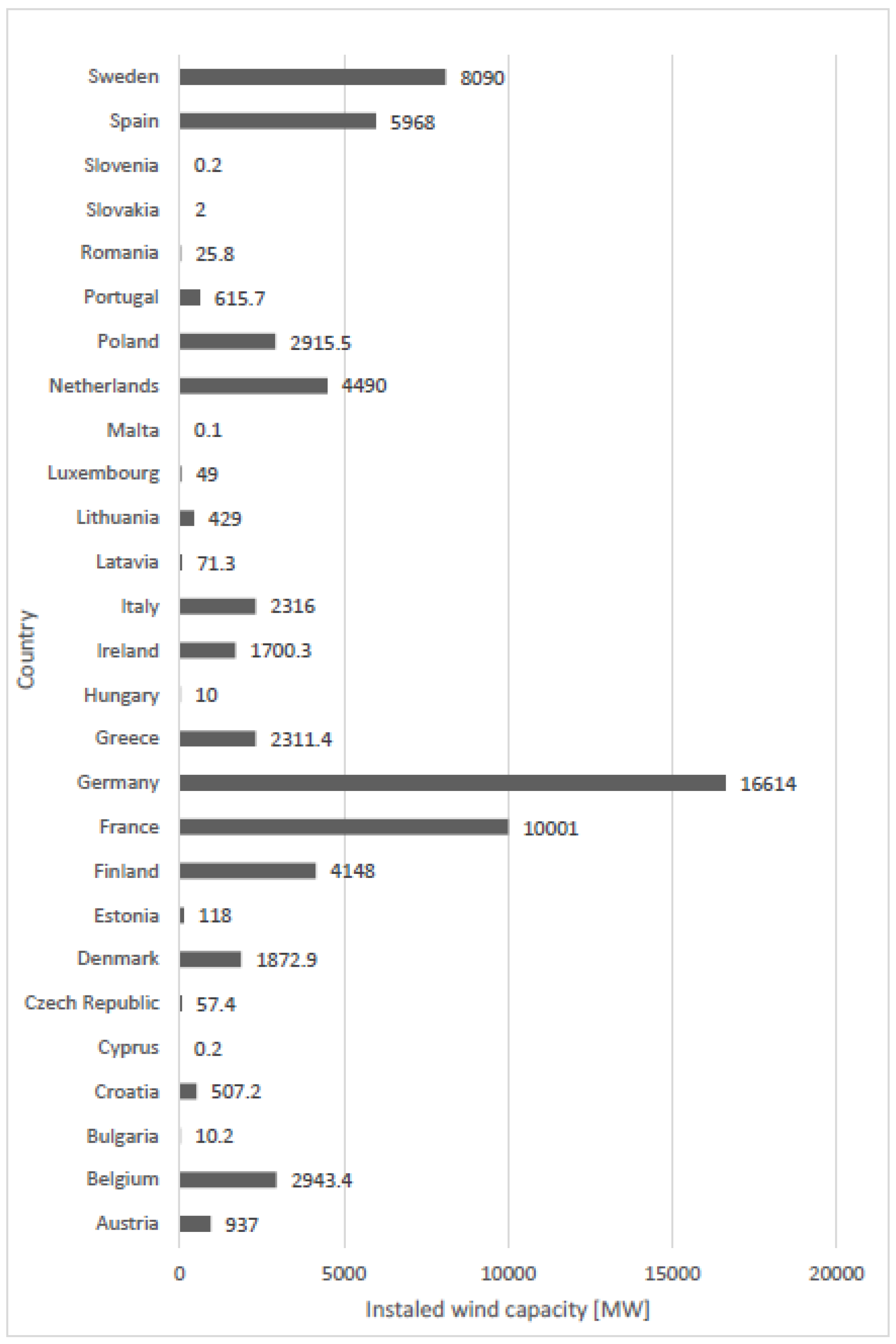
The report was compiled using data published annually in the Wind Energy Barometer, detailing the wind energy market trends in European Union member states, as shown in Figure 1.

In 2022, the growth of wind and solar energy installations remained high, continuing the momentum seen in 2021. An additional 75 GW of wind capacity and 191 GW of solar capacity were installed, driven primarily by China (+37 GW of wind and +86 GW of solar), the USA, and the EU. These efforts significantly boosted global renewable energy generation. The share of wind and solar energy in global electricity production increased by 1.5 percentage points, reaching over 12% in 2022, a significant rise from 2010 (+10 percentage points). Specifically, China saw a 2-point increase to 13.5%, while the USA’s share grew by 1.7 points, surpassing 14%. In Europe, the increase was more pronounced, with a rise of over three percentage points, bringing the total to nearly 22%. Notable gains were observed in countries like the Netherlands (+7.6 points) and Germany (+4.3 points), both exceeding 32%, as well as in Portugal, the UK, Poland, and Sweden (around +4 points each). Beyond these three major markets, the share of wind and solar in the energy mix also expanded in Australia (+3.6 points, reaching over 23%), Latin America (+1.7 points to 13%, with Chile up +5.4 points to 26% and Brazil up +2.9 points to 16%), and in Asia (+1.5 points to 12%, with wind and solar surpassing 10% in Japan and India). However, wind and solar energy remain marginal in Africa (5%, including 6% in South Africa), the Commonwealth of Independent States (CIS) (1%, with less than 1% in Russia and 6% in Ukraine), and the Middle East (less than 2%, despite increasing renewable generation in the United Arab Emirates) [8].

Accurate wind energy forecasting has become essential for the reliable integration of wind power into modern electricity grids [9]. Predictive models support grid operators by anticipating production variability, improving supply–demand balance, and enhancing overall grid stability [10,11]. A wide range of forecasting approaches has been proposed, including statistical, physical, and artificial intelligence (AI)-based methods. While statistical and physical models rely on historical data and atmospheric simulations, machine learning techniques increasingly dominate recent studies due to their ability to capture nonlinear relationships using large meteorological and production datasets [12].

The intermittency of wind energy also affects grid components, such as transformers, whose aging and degradation processes are difficult to predict due to variable operating conditions. Existing approaches typically combine forecasting models with detailed power system configurations to assess component stress and lifespan [13].

Numerous AI-based wind energy forecasting models have been reported in the literature. Artificial neural networks (ANNs) have been successfully applied for short-term energy prediction using meteorological inputs [14], while support vector machine (SVM)-based methods demonstrated improved performance compared to persistence models [15]. Hybrid approaches, such as SVM combined with metaheuristic optimization techniques, further enhanced prediction accuracy when tested on real wind farm data [16]. Other hybrid models, including ANFIS optimized with particle swarm optimization, achieved low prediction errors in short-term forecasting tasks [17]. Comparative studies indicate that machine learning models such as decision trees, nearest-neighbor regression, ANN, and SVM outperform linear regression techniques, with ANN-based models generally providing the highest accuracy at the cost of increased computational complexity [18]. Similar conclusions were reported in multi-model comparisons conducted on operational wind farms, confirming the effectiveness of AI-based approaches for wind energy prediction [19].

Several forecasting approaches focused on wind energy production in the Romanian context have been reported in the literature. For small-scale wind farms located in hilly regions of Romania, a two-step forecasting solution based on artificial neural networks was developed to improve hourly prediction accuracy, showing the potential of ANN-based models for local prediction tasks [20] (Lungu et al., 2016). In addition, machine learning techniques, including artificial neural networks, support vector machines, and decision tree models, have been applied to wind energy prediction in Romania, demonstrating that properly tuned ANN-based approaches can achieve high predictive accuracy, albeit with increased computational cost (Buturache and Stancu, 2021) [21]. Beyond neural network models, statistical methods such as the EGARCH model have been applied to analyze the volatility of wind energy production in Romania, offering insight into the variability and predictability of wind generation across the national grid [22].

This paper proposes a deep learning-based approach for predicting wind energy production in Romania by implementing feedforward neural networks and recurrent neural networks. Moreover, the theoretical fundamentals, data, and problem statement are explained in detail so that any other academics or professionals in the renewable energy field can replicate the experiment and later apply it to real-world scenarios. This study contributes by (i) providing a systematic benchmark comparison between FFNN and RNN models under identical experimental conditions, (ii) evaluating a large number of model configurations using national-scale operational data, and (iii) validating model robustness on multiple unseen time intervals. The focus is on reproducibility and practical forecasting performance rather than architectural novelty.

2. Materials and Methods

2.1. Input Data

As part of the effort made on the European Union level, Romania is continuously increasing its renewable energy production capacity. Compared to 1990, the running total of gas emissions cut at the European Union level is 32.5%. For 2022, the gas emissions decreased to a value around 3%, continuing a downward trend started 30 years ago [23]. The reduction in gas emissions is given, among other efforts, by the continuously increasing of renewable energy adoption. The target set in 2018 for the share of renewables in EU consumption for 2030 is 32%. In 2022, the share was 23% [24]. In 2024, the new adjusted target was 42.5%, but with good perspectives for 45% share of renewables in EU energy consumption. These achievements highlight the progress in meeting the climate and energy goals set for the next years, where resilience and sustainability are key. In line with the technological advancements and the need to accelerate the adoption of clean energy sources, Romania showed potential in many areas, including wind energy. One of the fastest-growing segments that added production capacity in Romania in 2023 was the prosumers [25]. At the beginning of 2023, the installed capacity accounted for by them was 417 MW, while by 1 July 2023, the installed capacity went up by more than double to 973 MW. Due to the grants offered by the government for photovoltaic panel installation and very favorable regulations, many people opted to become prosumers. Wind energy production data is made available in real time by Transelectrica [26]. Transelectrica SA is Romania’s sole operator, providing services of electricity transmission, operational technical management of the National Power System, and, by its subsidiary OPCOM (Romanian Power Market Operator, Bucharest, Romania), electricity market administration [27]. In order to have a full overview of the national energy mix, in addition to wind energy, the other energy sources are available through the same portal. Additionally, to understand the balance between supply and demand on a national level, information regarding the energy consumption across Romania is available too. Meteorological data is key to delivering accurate wind energy production. Given the growing number of business use cases in the areas where meteorological data is used, but not limited to renewable energy, nowadays, there are very reliable weather application programming interface (API) services available [28].

The dataset considered for the modeling consists of hourly data taken between 1 January 2023 and 31 December 2023 for both meteorological and production data. The API used proved to deliver data free of any quality problems, while the data for wind energy production had some missing records.

Table 1. Input data statistics.

	Availability [%]	Mean	std	Min	25%	50%	75%	Max
Temperature [C]	100	14.4	9.7	−8.1	6.3	14	21.8	40.7
Real feel [C]	100	14.1	10.1	−8.7	5.6	14	21.8	40.7
Dew Point [C]	100	7.4	6.4	−12.2	2.7	7.5	12.6	24.3
Humidity [%]	100	67.7	21.6	13.4	49.5	69.3	86.7	100
Precipitations [mm]	100	0.0	0.5	0	0	0	0	20.2
Snow Depth [mm]	100	0.2	0.9	0	0	0	0	10.7
Wind Gust [km/h]	100	17.6	10.3	0.7	9.4	15.8	24.1	65.9
Wind Speed [km/h]	100	4.7	3.4	0	3.6	3.8	7.2	31.4
Wind Direction [degrees]	100	149.3	106.7	0	50	127	240	360
Pressure [mb]	100	1015.8	7.6	989.4	1011.3	1015.6	1020.3	1044.7
Cloud Cover [%]	100	56.3	38.7	0	14.4	60.1	97.4	100
Visibility [km]	100	10.1	2.4	0	10	10	10.2	60.7
Solar Radiation [W/m2]	100	10.7	51.6	0	0	0	3	850
Wind energy [MW]	99.8	850.6	694.0	0	278.5	667	1300	2766

presents the statistics of the input data for both weather and production. The missing data for wind energy production will be imputed as part of the data preprocessing step. However, given that missing wind energy production values accounted for less than 0.2% of the dataset and occurred in short, isolated gaps, model performance is expected to be largely insensitive to the imputation method. Linear interpolation preserves local temporal continuity without introducing artificial bias; therefore, a dedicated sensitivity analysis was not considered necessary.

In addition to the meteorological variables listed in Table 1, a derived feature representing freezing rain events was introduced during data preprocessing. Freezing rain was identified based on the simultaneous occurrence of precipitation and air temperatures below 0 °C. This phenomenon is particularly relevant for wind energy production, as ice accretion on turbine blades alters the airfoil shape, degrades aerodynamic performance, and can lead to power losses or temporary turbine shutdowns. By explicitly accounting for freezing rain conditions, the model is better equipped to capture atypical production drops associated with adverse winter weather events.

This type of event has big implications in wind energy production due to the fact that the layer of ice settling on the blade airfoil degrades its aerodynamic performance.

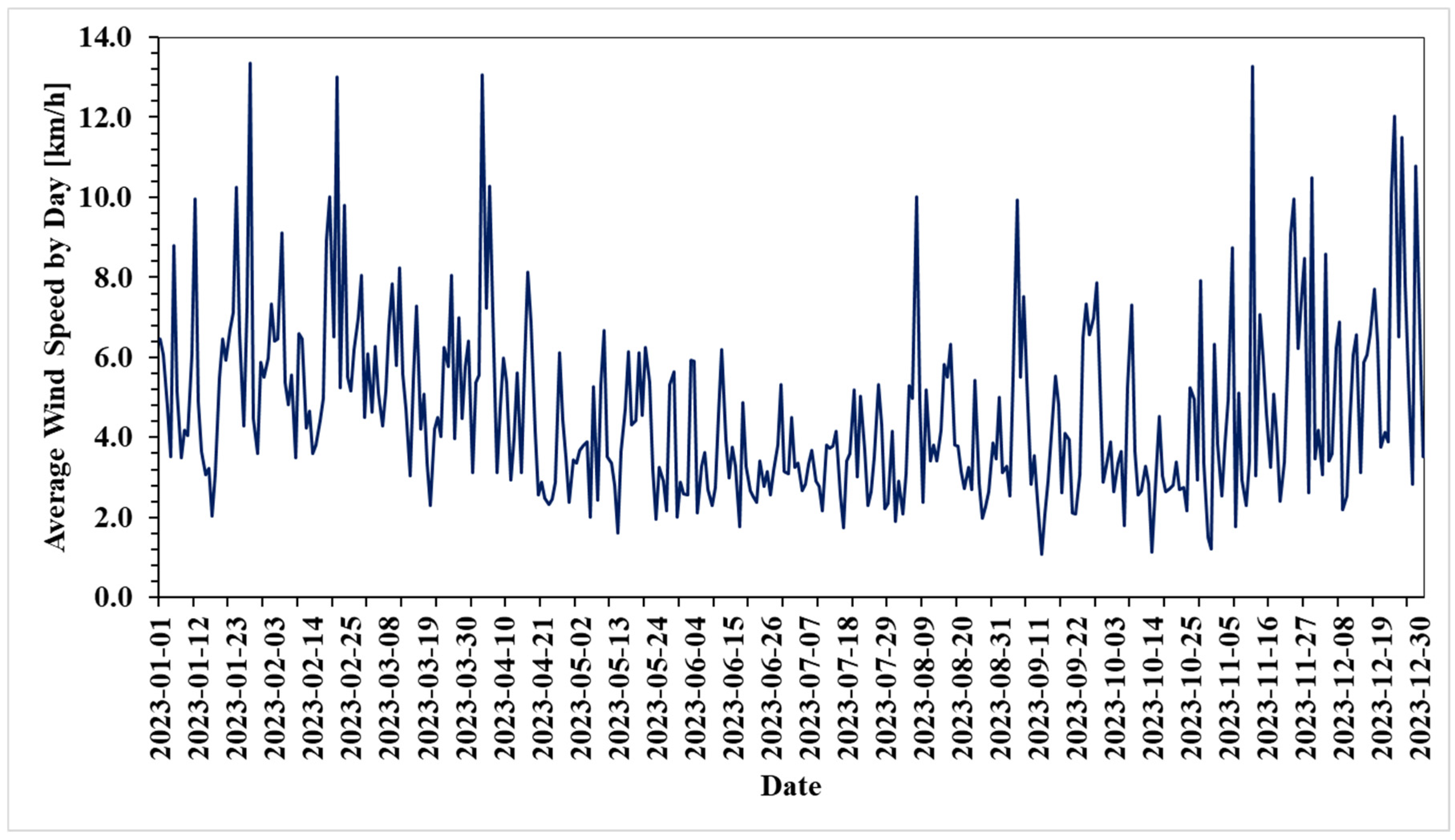
One of the most important downsides of wind energy is given by its volatility. As can be seen in Figure 2, throughout the considered timeframe, the average wind speed varies a lot. This behavior, dominated by intermittency, is impacting wind energy production.

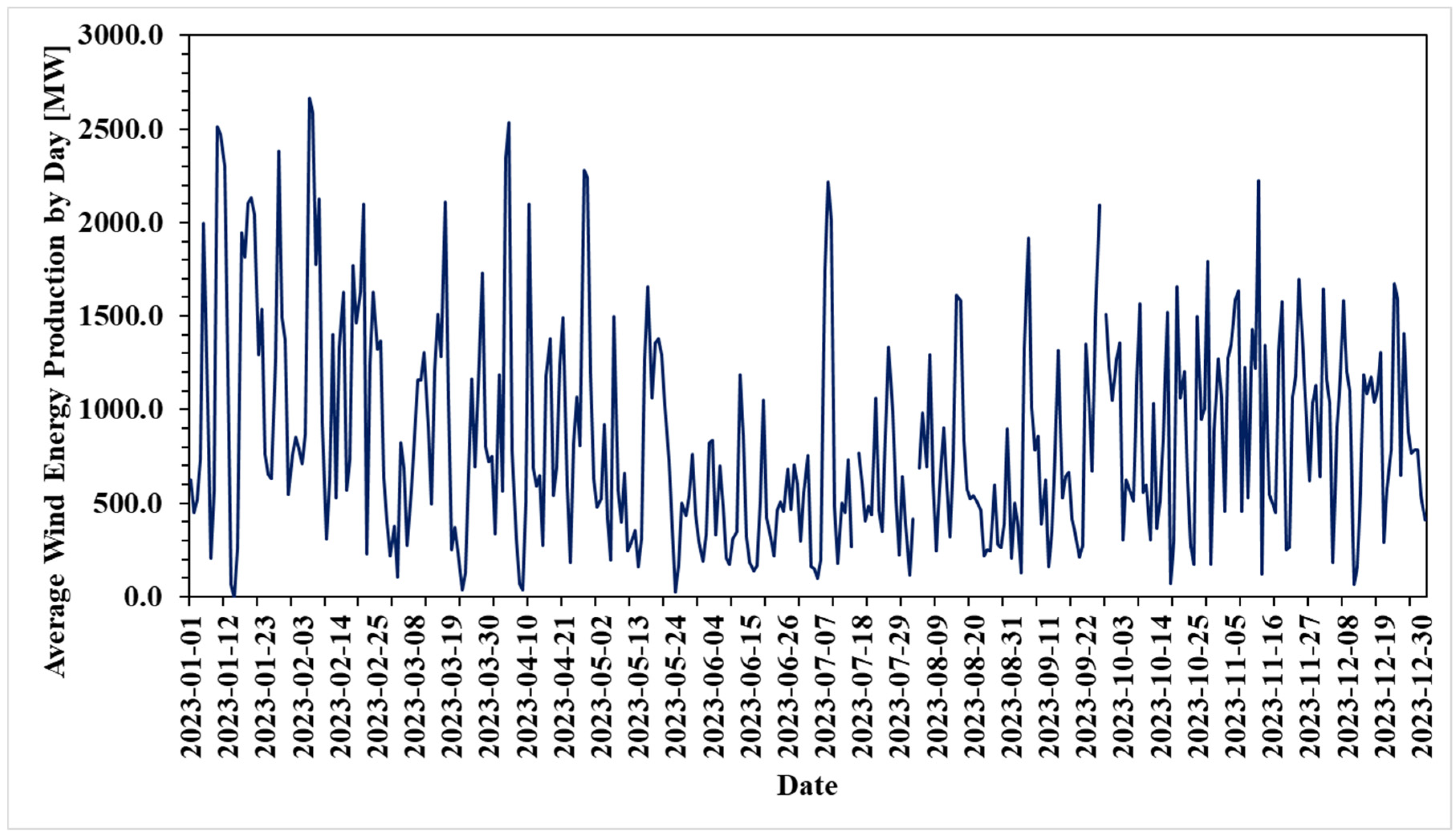
The volatility of wind energy production is presented in Figure 3. Any grid should be stable, predictive, and capable of keeping up with demand. By increasing the adoption of wind energy on a large scale, the need to know upfront how much it will impact the key performance metrics of the grid is key.

2.2. Theoretical Fundamentals

The neurons composing artificial neural networks are inspired by biological neurons. A biological neuron is the building block of the brain, specialized in processing information. Information is received as an electrical impulse, processed, and then the signals generated after processing are propagated further.

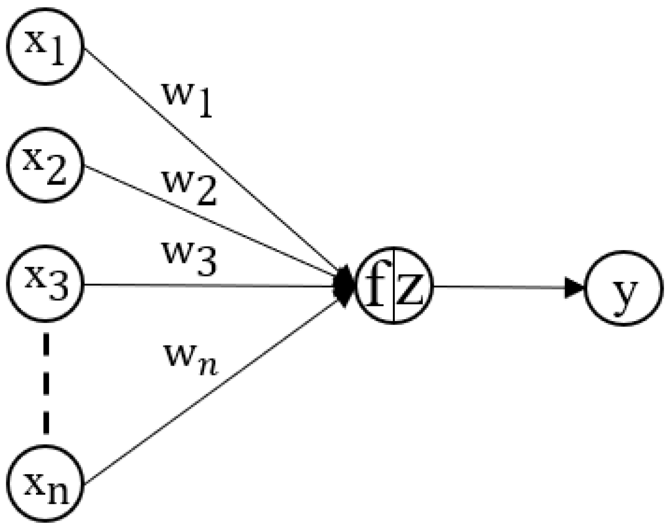
The artificial neural network concept was presented for the first time in 1943 by McCulloch and Pitts [29], with the main purpose of replicating the mechanisms that were expected to be found in the human brain. As with a biological neuron, each artificial neuron has its own vector of inputs ${(\mathrm{x}}_1,{\mathrm{x}}_2,\dots ,{\mathrm{x}}_{\mathrm{n}}) \in {\mathrm{R}}^{\mathrm{n}}$, with each input having its own importance represented by the weights vector ${(\mathrm{w}}_1,{\mathrm{w}}_2,\dots ,{\mathrm{w}}_{\mathrm{m}}) \in {\mathrm{R}}^{\mathrm{m}}$. The simplified logic is presented in Figure 4.

Weight values modulate the importance of the input, so all inputs and associated weights are computed as a weighted sum (Equation (1)):

$$\mathrm{z} = \sum _{\mathrm{i}=1}^{\mathrm{n}}{\mathrm{x}}_{\mathrm{i}}{\mathrm{w}}_{\mathrm{i}}$$

(1)

To the weighted sum of the inputs, $\mathrm{z}$ is applied to the activation function, $\mathrm{f}$. By design, a neuron can be activated only if a certain threshold is exceeded. In this way, the activation function moderates the signals transmitted further. The output value of a neuron, $\mathrm{y}$, is obtained as in Equation (2):

$$\mathrm{y} = \mathrm{f}\left(\mathrm{z}\right) = \mathrm{f}(\sum _{\mathrm{i}=1}^{\mathrm{n}}{\mathrm{x}}_{\mathrm{i}}{\mathrm{w}}_{\mathrm{i}})$$

(2)

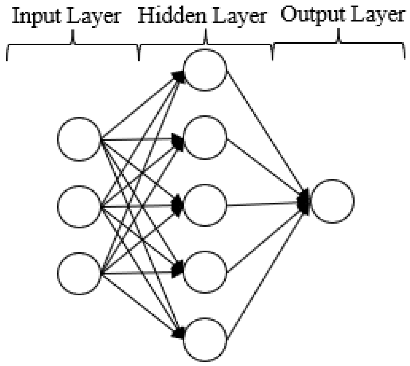
A multilayer perceptron is a type of artificial neural network consisting of an input layer, one or more hidden layers, and an output layer. A layer consists of multiple neurons (Figure 5), and neurons on consecutive layers are fully connected. The input layer and output layer communicate with the outside world, while information is propagated through the network from the input to the output layer. This concept became feasible when backpropagation began to be used [30]. Using backpropagation during training, the synaptic weights are adjusted based on a statistical criterion, taking into consideration both actual and expected predictions. In this way, inputs receive the right weight with respect to the studied problem, meaning that they contain the knowledge gained during the training.

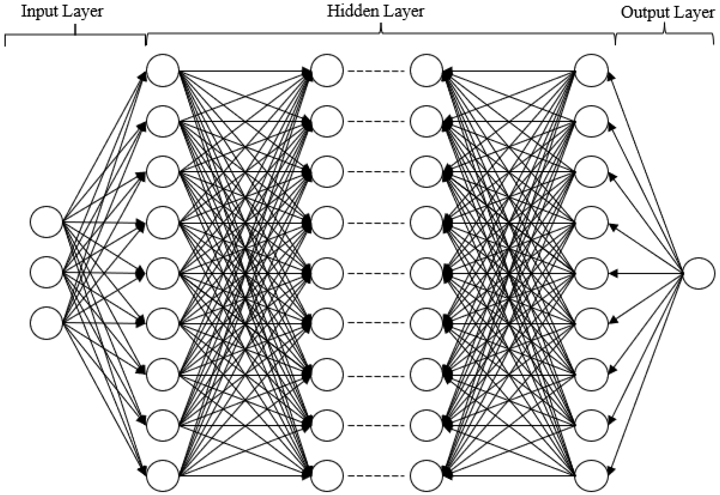
Deep neural network architecture is based on the multilayer perceptron, but with additional layers and an increased number of neurons on each layer (Figure 6). By increasing both the number of layers and the number of neurons, the overall capacity of the network to acquire knowledge is increased. The downside of it is that training time will be increased by epoch, and solution convergence might require more epochs.

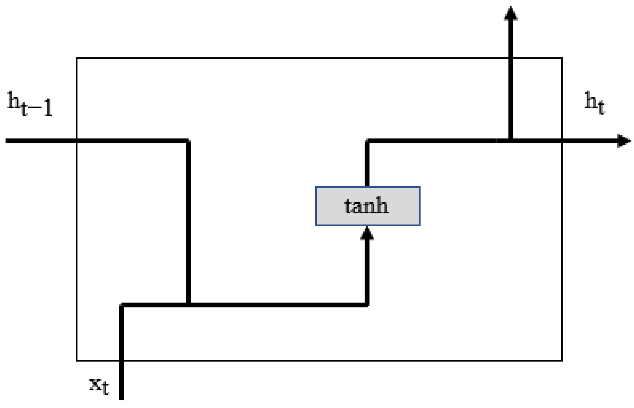
Standard recurrent neural networks (RNNs) are designed to process sequential data such as time series or text (Figure 7). These types of problems are needed to generate a prediction with respect to the previous time steps.

This type of recurrent neural network can be defined as follows [31]:

$${\mathrm{h}}_{\mathrm{t}} ={\mathrm{f}}_{\mathrm{h}}\left({\mathrm{x}}_{\mathrm{t}},{\mathrm{h}}_{\mathrm{t}-1}\right) = {\mathsf{\varphi }}_{\mathrm{h}}({\mathrm{W}}^{\mathrm{T}}{\mathrm{h}}_{\mathrm{t}-1} + {\mathrm{U}}^{\mathrm{T}}{\mathrm{x}}_{\mathrm{t}})$$

(3)

$${\mathrm{y}}_{\mathrm{t}}={\mathrm{f}}_{\mathrm{o}}\left({\mathrm{h}}_{\mathrm{t}},{\mathrm{x}}_{\mathrm{t}}\right)={ \mathsf{\varphi }}_{\mathrm{o}}\left({\mathrm{V}}^{\mathrm{T}}{\mathrm{h}}_{\mathrm{t}}\right)$$

(4)

where ${\mathrm{f}}_{\mathrm{h}}$ and ${\mathrm{f}}_{\mathrm{o}}$ are activation functions, ${\mathrm{x}}_{\mathrm{t}}$ and ${\mathrm{y}}_{\mathrm{t}}$ are input and output vectors, and ${\mathrm{h}}_{\mathrm{t}-1}$ and ${\mathrm{h}}_{\mathrm{t}}$ are the hidden states for the previous step and current step. As for the multilayer perceptron, the elements that are gaining knowledge during the training are the synaptic weights represented by the vectors W, U, and V. Based on Equation (3), at the current time step, t, the new information received at this time step, ${\mathrm{x}}_{\mathrm{t}}$, is concatenated with the information kept from the previous hidden state, ${\mathrm{h}}_{\mathrm{t}-1}$. Thus, the new vector contains both new information from the current time step and relevant information from the past. By applying the hyperbolic tangent activation function, the values in the current state are bounded between −1 and 1. The same reasoning is applied to the output at the current step, ${\mathrm{y}}_{\mathrm{t}}$, as in Equation (4).

When model performance is discussed, there are two aspects to be considered. The first one, pure model performance, is independent of the used dataset. Coefficient of determination (${\mathrm{R}}^2$) is a measure of how well the model can explain the variability of the outcome, Equation (5), where $\widehat{{\mathrm{y}}_{\mathrm{i}}}$ and ${\mathrm{y}}_{\mathrm{i}}$ are the predicted values and actual values. The minimum value is 0, and the maximum is 1. The higher the value, the better the performance. The second aspect to be considered is how the performance is expressed in order to be sensed by the subject matter experts or end users. By using mean absolute error (MAE), the metric is dependent on the data used, averaging the absolute values of the prediction errors (Equation (6)):

$${\mathrm{R}}^2 = 1 - {\displaystyle \frac{{\sum }_{\mathrm{i}=1}^{\mathrm{n}}\left({\mathrm{y}}_{\mathrm{i}} - \widehat{{\mathrm{y}}_{\mathrm{i}}}\right)}{{\sum }_{\mathrm{i}=1}^{\mathrm{n}}{\left({\mathrm{y}}_{\mathrm{i}} - \widehat{{\mathrm{y}}_{\mathrm{i}}}\right)}^2}}$$

(5)

$$\mathrm{MAE}={\displaystyle \frac{1}{\mathrm{n}}}\sum _{\mathrm{i}=1}^{\mathrm{n}}|{\mathrm{y}}_{\mathrm{i}} - \widehat{{\mathrm{y}}_{\mathrm{i}}}|$$

(6)

Artificial neural networks, in general, are highly configurable models where selecting the right hyperparameters can make the difference between good and outstanding performance. Hyperparameter tuning is the process of adjusting the network’s parameters and architecture. The goal of hyperparameter tuning is to find the global optimum for which the model’s performance is the best for the given use case. This process is time- and resource-consuming, and most of the time it involves a lot of experimentation and very well-defined techniques like random search, grid search, or Bayesian optimization. Since this research falls under the supervised machine learning paradigm, it is crucial to split the dataset into training and testing subsets. The training subset consists of 90% of the dataset, while the remaining 10% is kept for testing purposes. The training subset is used for learning, where the model acquires knowledge about the patterns within the data, while the testing subset is used to test the model’s capability to generalize to new, unseen data. This approach ensures that the model’s performance is evaluated not only on the cases in the training subset, but also on other data, reasonably assuming that the training dataset is not the exhaustive list of situations that can be encountered during real-world scenarios.

Unlike the synaptic weights that are only initiated based on reasoning, but later updated according to the model’s calculated error, the hyperparameters defining the network must be predefined before the training begins. The hyperparameters considered for training are available in

Table 2. FFNN and RNN tested hyperparameters.

Hyperparameter	Model Type	Values
Batch size	Feedforward, RNN	256, 512, 1024
Epochs	Feedforward, RNN	30, 50, 70
Activation function	Feedforward, RNN	Sigmoid, Rectified linear unit
Optimizer	Feedforward, RNN	Rmpsprop, Adam, Adagrad
Weights initialization	Feedforward, RNN	Lecun normal, Lecun uniform, Xacier normal, Xavier uniform
Number of hidden layers	Feedforward	2
	RNN	1
Number of neurons on hidden layers	Feedforward, RNN	53, 105, 210
Learning rate	Feedforward, RNN	0.001

.

The hyperparameter ranges reported in Table 2 were selected based on a combination of established practices in neural-based models and practical considerations related to dataset size and computational efficiency. Batch sizes were selected as powers of two to ensure computational efficiency and compatibility with GPU-based training, which is in line with common deep learning practice. The number of epochs was chosen to allow sufficient learning while limiting overfitting, as preliminary tests indicated convergence within this range. Activation functions, optimization algorithms, and weight initialization strategies were selected from widely adopted and well-documented options to ensure robustness and reproducibility.

In total, we trained and tested 1296 models for both architectures.

3. Results and Discussion

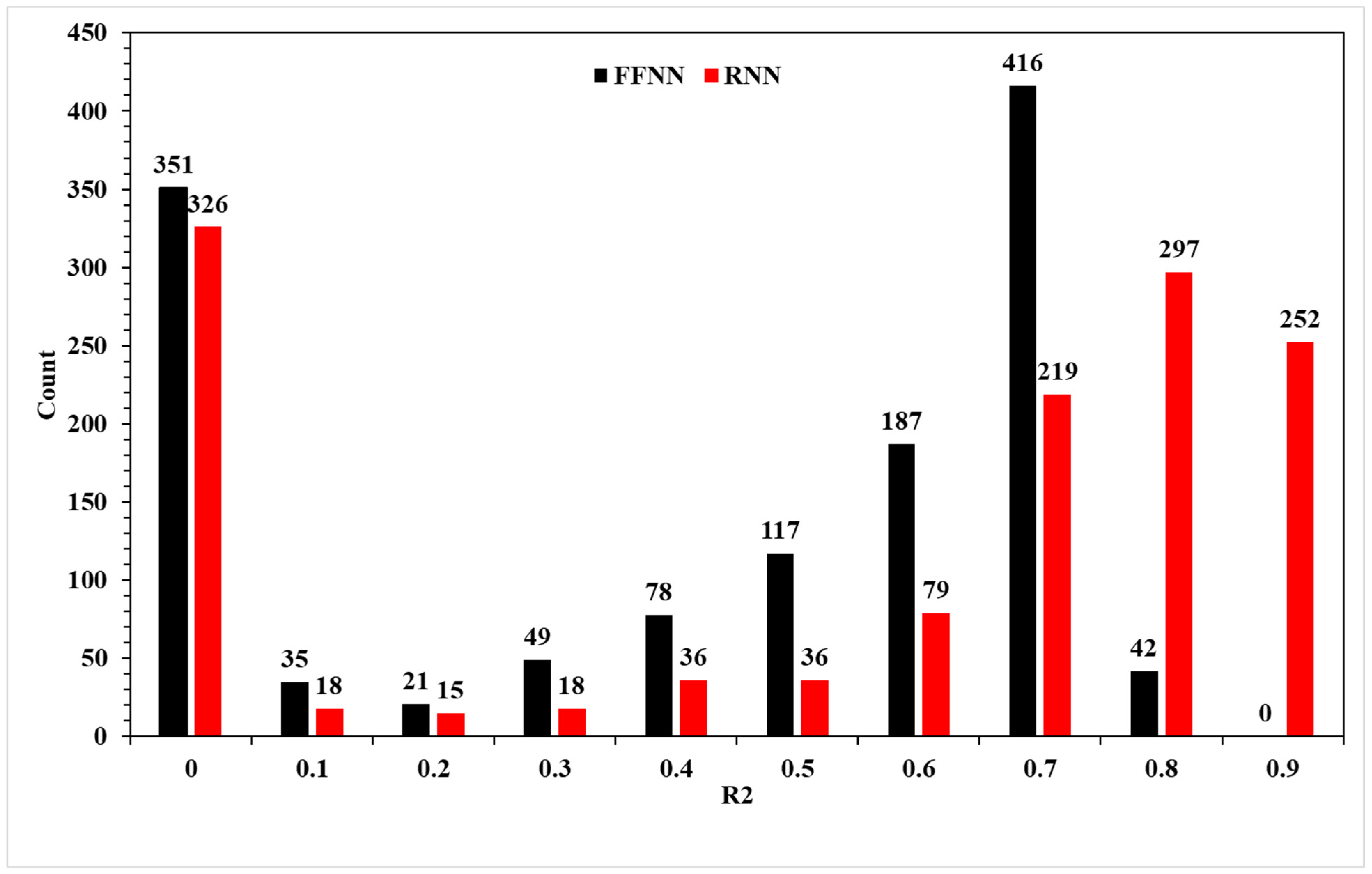
The results of the study are in line with RNN and feedforward neural network characteristics, providing very good performance for a wide range of hyperparameters. This is confirmation of the fact that the generalization capabilities of both architectures can handle prediction tasks even though the hyperparameter selection is not perfect for the use case. By globally assessing how well the models were built and performed, it is clear that for time-series data, RNNs have some extra prediction capabilities compared to FFNNs (Figure 8).

Figure 7 presents a comparative distribution of the FFNN and RNN model performances across various R² intervals. The histogram illustrates the number of models (out of 1296) that fall within specified R² ranges, thereby offering insight into the consistency and generalization ability of each architecture.

It is evident that RNN models outperform FFNN models in the higher R² ranges. Specifically, while FFNNs show a sharp concentration in the lower range (R² = 0), with 351 models, RNNs demonstrate better learning and prediction capabilities, with only 326 models falling in the same lowest category. More notably, RNNs dominate the higher ranges: 219 models achieve R² between 0.7 and 0.8, and 252 models exceed R² of 0.8. In contrast, FFNNs record only 42 models in the 0.8–0.9 range and none above 0.9, indicating limited capacity to achieve high accuracy on unseen data.

This distribution highlights the superior generalization of RNNs when dealing with time-series data, as over 42% of RNN models surpass the R² threshold of 0.80. This also suggests that RNNs, due to their inherent capability to capture temporal dependencies, are more robust in modeling wind energy variations over time compared to feedforward architectures.

Figure 8 quantitatively supports the claim that RNNs exhibit enhanced predictive power and reliability, especially in high-accuracy scenarios, which is critical for applications such as short-term wind power forecasting.

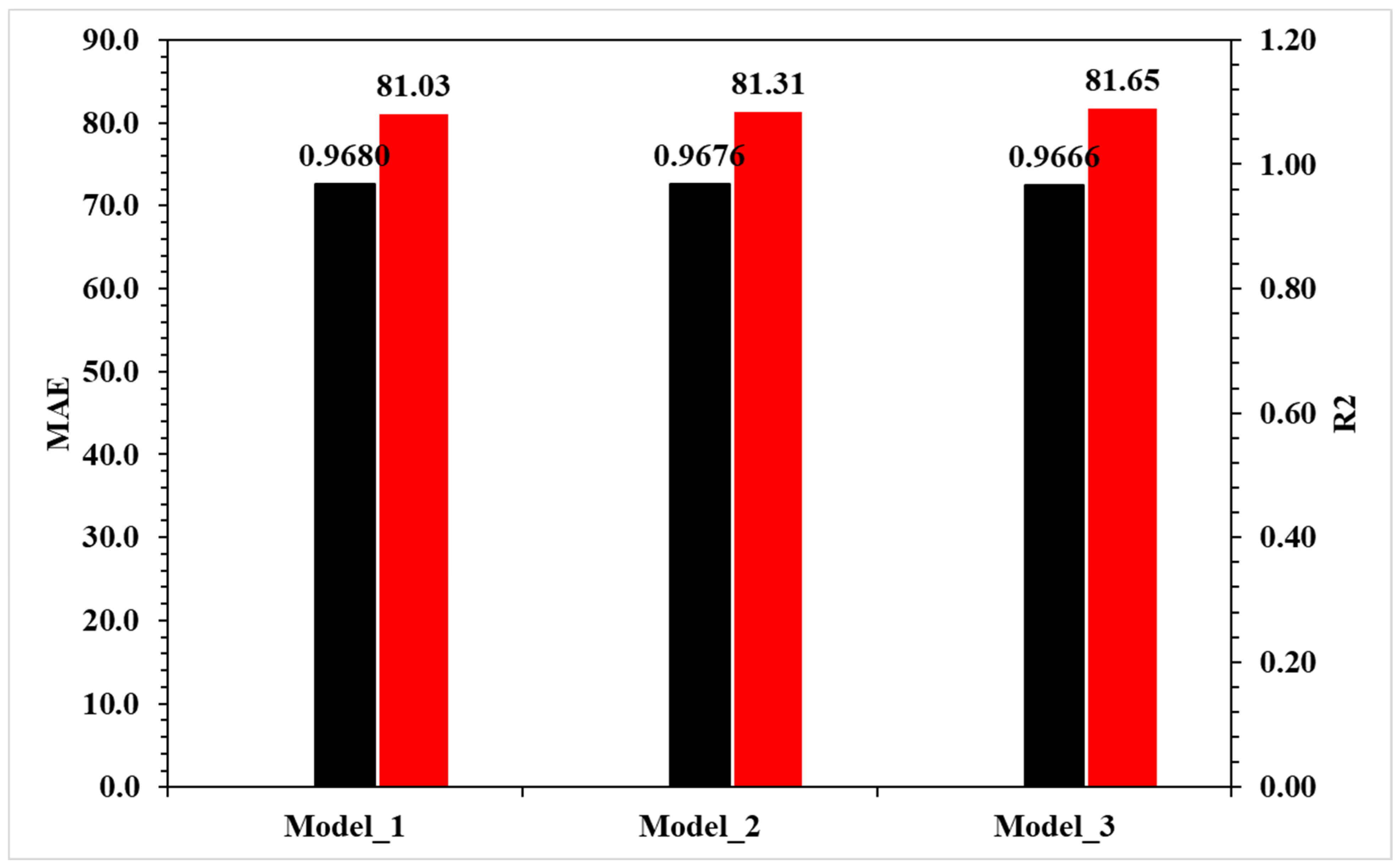
In terms of performance, the top three models are described in

Table 3. Hyperparameters of top 3 models by performance.

Model	Hyperparameters	${\mathbf{R}}^2$	MAE
1	batch = 128, epochs = 30, activation = tanh, opt = adam, wi = glorot uniform, nl = 2, nn1 = 196, nn2 = 49;	0.9680	81.03
2	batch = 128, epochs = 50, activation = sigmoid, opt = rmsprop, wi = lecun uniform, nl = 2, nn1 = 196, nn2 = 98;	0.9676	81.31
3	batch = 128, epochs = 50, activation = sigmoid, opt = rmsprop, wi = lecun normal, nl = 2, nn1 = 49, nn2 = 98;	0.9666	81.65

batch = batch size, epoch = number of epochs, activation = activation function, opt = optimization algorithm, wi = weights initialization, nl = number of layers, and nnx = number of neurons on the x hidden layer.

and Figure 9.

Table 3 and Figure 9 present a detailed comparison of the top three performing neural network models based on their respective R² (coefficient of determination) and MAE (mean absolute error) values. All three models share common hyperparameters in terms of number of hidden layers (2) and batch size (128), indicating that these two factors are particularly influential in achieving high predictive performance. These constants suggest that an optimal batch size and architectural depth are essential when forecasting wind power with deep learning models.

The variation among the models lies in other hyperparameters such as the activation function, weight initialization, and the number of neurons in each hidden layer. However, as noted in the manuscript, it is difficult to isolate a single parameter as dominant; rather, proper tuning within well-defined ranges during the optimization process allows each configuration to reach high accuracy.

Figure 8 illustrates the performance metrics of the top three models. Model 1, using a tanh activation function and Adam optimizer, achieved the best performance with an R² value of 0.9680 and an MAE of 81.03 MW. Models 2 and 3, both using sigmoid activations and the RMSprop optimizer, followed closely with R² values of 0.9676 and 0.9666, and MAE values of 81.31 MW and 81.65 MW, respectively.

The differences in performance are minimal—less than 0.002 in R² and less than 1 MW in MAE—confirming the robustness of the models and validating the consistency of the deep learning approach under varying hyperparameter configurations. These results also reinforce that RNN-based architectures, when properly tuned, can deliver accurate wind energy forecasts, with an error margin of under 4.5% relative to the mean output (~850 MW).

In conclusion, both Table 3 and Figure 9 demonstrate that small variations in configuration can still yield comparably high accuracy, provided the architectural backbone (layers and batch size) remains optimal. These insights are valuable for future deployments where computational efficiency and model interpretability may guide hyperparameter selection.

A quantitative comparison between the best-performing RNN and FFNN models indicates that recurrent architectures consistently achieve lower prediction errors. Specifically, the optimal RNN configuration reduces the mean absolute error (MAE) by approximately 12–15% compared to the best FFNN models, while also achieving a reduction in root mean square error (RMSE) of up to 20%. These improvements highlight the advantage of capturing temporal dependencies when forecasting wind energy time series.

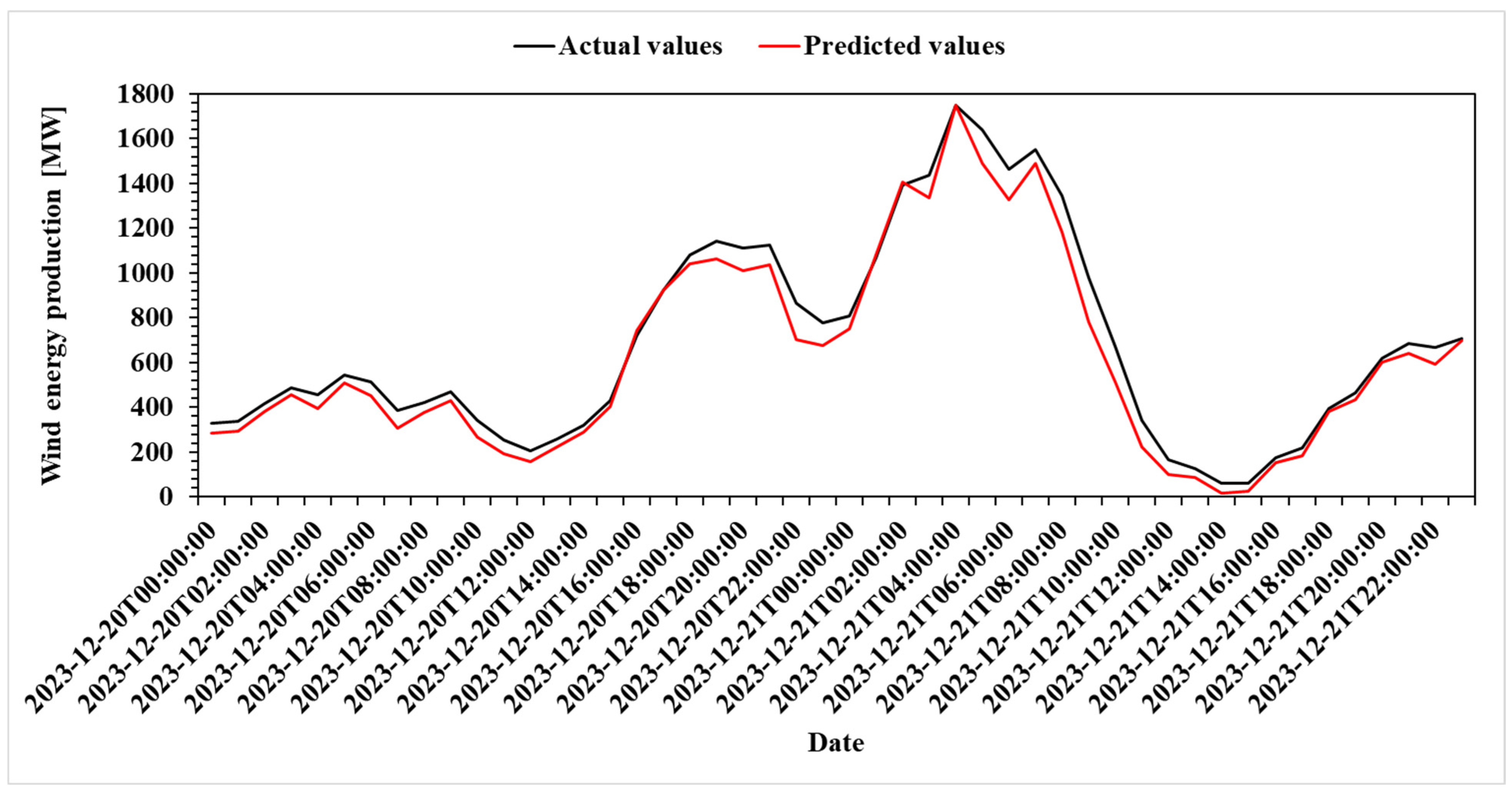
Another way to assess model performance can be done in a qualitative manner by plotting the actual values recorded against the predicted values. For Model_1, the time interval between 2023-12-20T00:00:00 and 2023-12-21T23:59:59 is selected (Figure 10). This time interval is selected out of the testing subset, being a representation of how well the model can generalize to unseen data.

Figure 10 provides a qualitative assessment of the predictive performance of Model_1 by comparing actual wind energy production values with the corresponding predicted values over a 48 h period, specifically between 2023-12-20T00:00:00 and 2023-12-21T23:59:59. This interval was selected from outside the original training and validation datasets, offering a clear indication of the model’s generalization capability on unseen data.

The comparison reveals a close alignment between the actual (black line) and predicted (red line) values, with the model successfully capturing the overall trend, peak structures, and local variations in the wind power output. Notably, the model responds well to both ascending and descending slopes of the power curve, reflecting its ability to follow the natural volatility of wind energy generation.

While minor deviations are visible—particularly around the peak value near midday on December 21—the predicted curve remains within acceptable bounds and does not exhibit systematic lag or phase shifting, which is a common drawback in time-series forecasting models. The slight overestimation near the peak may be attributed to dynamic meteorological fluctuations not fully captured by the input variables.

Overall, Figure 10 confirms that Model_1 demonstrates strong temporal learning and prediction stability under real-world conditions. The qualitative match between actual and predicted values supports the previously observed quantitative metrics (e.g., R² = 0.9680, MAE = 81.03 MW) and reinforces the suitability of the selected model architecture for short-term wind energy forecasting.

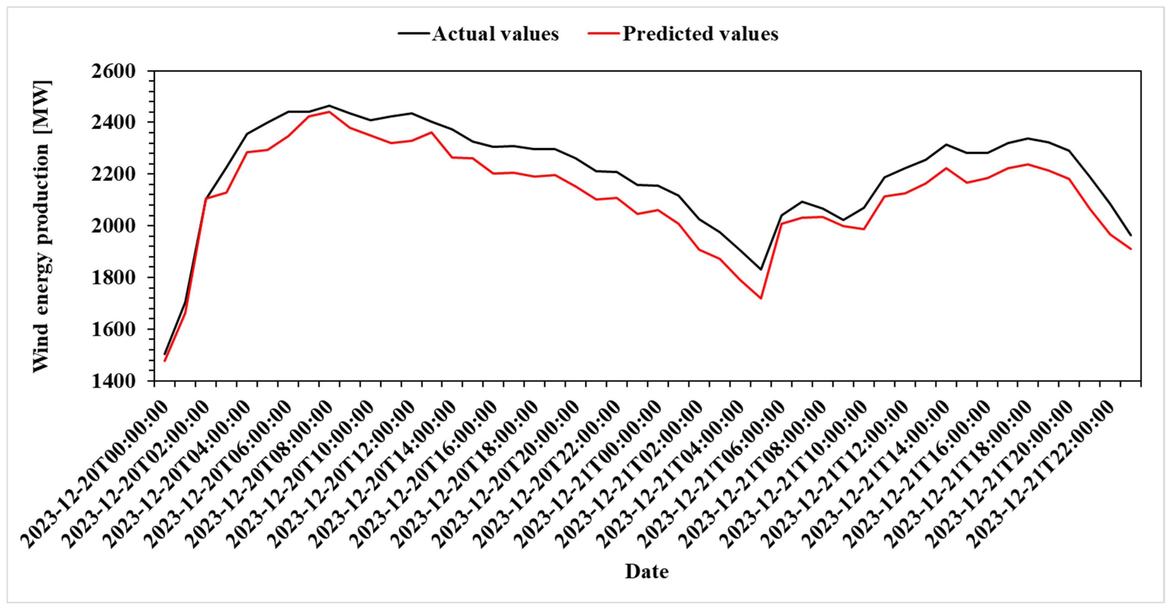
Another meaningful analysis is to see how the model performs for a time interval outside the one considered for testing. In an attempt to simulate a scenario as close as possible to a real-world one, Figure 11 plots the actual values against the predicted values of the same Model_1, but for the time interval from 2024-03-15T00:00:00 to 2024-03-16T23:59:59.

Figure 11 illustrates a complementary evaluation of Model_1’s robustness by testing it on a new time interval entirely outside the original test set, namely from 2024-03-15T00:00:00 to 2024-03-16T23:59:59. This scenario simulates real-world applicability, where the model must forecast wind energy based on future unseen conditions.

The visual comparison between actual values (black line) and predicted values (red line) reveals that Model_1 maintains a high level of prediction accuracy. The model successfully tracks the general shape and amplitude of the production curve, including the initial steep increase and subsequent peak values above 2400 MW. Moreover, the prediction maintains coherence with the actual trend, even in areas of sharp curvature and inflection, such as the minor drop occurring mid-interval.

Despite this, a slight systematic underestimation is noticeable across most of the time span, particularly in the plateau and descending segments. This may suggest a conservative bias of the model under high wind energy conditions, possibly due to limitations in the training data’s variability range or incomplete representation of extreme weather scenarios in the input features.

The high R² values and low MAE obtained indicate strong overall predictive performance across the full range of observed wind power values. This suggests that, at the national and hourly aggregation levels considered, wind energy production exhibits a high degree of short-term predictability. Such predictability does not eliminate inherent variability but can reduce operational uncertainty and support grid scheduling and reserve planning.

Nevertheless, the absence of abrupt prediction failures and the overall close tracking of actual values demonstrate that the model generalizes effectively, even when applied to time windows far removed from the training context. The consistency of prediction performance across multiple time intervals further validates the model’s reliability for short-term forecasting tasks in operational energy systems.

Analyzing Figure 10 and Figure 11, it can be observed that the model tends to slightly underestimate the wind energy production compared to actual values. And yet, the performance of the model remains high, and the difference between actual values and predicted values is very small.

The results of this study are consistent with, and extend beyond, previous wind energy forecasting research conducted both in Romania and at the international level. Lungu et al. [20] demonstrated the applicability of ANN-based models for small-scale wind farms in hilly regions of Romania, focusing on localized forecasting accuracy. In contrast, the present work evaluates a substantially larger model space, including both FFNN and RNN architectures, validated at a national scale and across multiple unseen time intervals.

Compared to the machine learning-based study of Buturache and Stancu [21], which analyzed ANN, SVM, and decision tree models, the present research advances the state of the art by explicitly modeling temporal dependencies through recurrent neural networks and by systematically quantifying accuracy–computational cost trade-offs. Statistical approaches, such as the EGARCH-based volatility analysis proposed by Murărașu [22], provide valuable insights into production variability, but do not directly address short-term operational forecasting, which is the primary focus of this work.

At the international level, several studies have reported the effectiveness of advanced deep learning architectures for wind power forecasting, including LSTM- and GRU-based models and hybrid frameworks ([32,33,34]). While these approaches often achieve high accuracy, they are typically evaluated on limited datasets or specific wind farms. The present study differentiates itself through a large-scale, reproducible comparison of FFNN and RNN models using real operational data and by emphasizing robustness, generalization, and practical applicability for power system operation.

Despite the strong predictive performance, several limitations should be noted. The study is restricted to standard FFNN and RNN architectures and to a single national dataset, which may limit direct generalization to other regions or climates. In addition, more advanced architectures such as LSTM or GRU were not considered. These limitations point to future research directions focused on broader geographical validation and the inclusion of more expressive temporal models.

4. Conclusions

This study assessed the performance of deep learning models—specifically feedforward neural networks (FFNNs) and recurrent neural networks (RNNs)—for wind energy prediction, with emphasis on accuracy, generalization, and interpretability. The results indicate that RNNs consistently outperform FFNNs within the investigated experimental setup, achieving a reduction in mean absolute error (MAE) of approximately 12–15%, depending on the dataset.

The analysis of input variables suggests that wind speed and wind direction are the most influential factors affecting prediction accuracy. Incorporating these variables as primary inputs led to a reduction in root mean square error (RMSE) of up to 20% compared to baseline model configurations without explicit feature selection.

While RNN-based models achieved higher predictive accuracy, they also required increased computational resources. For example, the optimal RNN configuration required approximately 4 h of training time on a standard GPU setup, compared to around 40 min for the best-performing FFNN model, highlighting a trade-off between model complexity and deployment efficiency.

Wind power forecasting remains a challenging task due to the inherent intermittency of wind. Nevertheless, even moderate reductions in forecasting error (on the order of 5–10%) can have meaningful operational benefits, including improved grid stability and reduced reliance on backup generation from conventional sources.

From an operational perspective, the proposed forecasting framework has the potential to support real-world power system operation by assisting short-term scheduling, reserve allocation, and grid balancing decisions. Hourly wind power forecasts may be used by transmission system operators and wind farm operators to anticipate production variability and improve coordination with other energy sources, particularly under increasing wind energy penetration.

It should be noted that the present validation is limited to a single national dataset and a specific temporal scope. Consequently, while the results demonstrate promising accuracy, generalization within this context, broader validation across multiple geographical regions, longer time horizons, and additional model architectures are required to fully assess robustness. More complex architectures were intentionally excluded in order to maintain a controlled and reproducible comparison with lower computational complexity. Future work will therefore focus on extending the framework through the integration of more advanced recurrent architectures, such as Long Short-Term Memory (LSTM) and Gated Recurrent Unit (GRU) networks, as well as by incorporating turbine operational parameters, high-resolution meteorological data, and hybrid or physics-informed modeling approaches.

References

1. European Commission. The European Green Deal. Available online: https://commission.europa.eu/strategy-and-policy/priorities-2019-2024/european-green-deal_en (accessed on 1 March 2025).
2. Avtar, R.; Sahu, N.; Aggarwal, A.K.; Chakraborty, S.; Kharrazi, A.; Yunus, A.P.; Dou, J.; Kurniawan, T.A. Exploring Renewable Energy Resources Using Remote Sensing and GIS—A Review. Resources 2019, 8, 149. [Google Scholar] [CrossRef]
3. Loth, E. Wind energy value and deep decarbonization design: What’s next? Next Energy 2023, 1, 100059. [Google Scholar] [CrossRef]
4. Boadu, S.; Otoo, E. A comprehensive review on wind energy in Africa: Challenges, benefits and recommendations. Renew. Sustain. Energy Rev. 2024, 191, 114035. [Google Scholar] [CrossRef]
5. Ayua, T.J.; Emetere, M.E. Technical analysis of wind energy potentials using a modified Weibull and Raleigh distribution model parameters approach in the Gambia. Heliyon 2023, 9, e20315. [Google Scholar] [CrossRef]
6. Nassar, Y.F.; El-Khozondar, H.J.; El-Osta, W.; Mohammed, S.; Elnaggar, M.; Khaleel, M.; Ahmed, A.; Alsharif, A. Carbon footprint and energy life cycle assessment of wind energy industry in Libya. Energy Convers. Manag. 2024, 300, 117846. [Google Scholar] [CrossRef]
7. Wolniak, R.; Skotnicka-Zasadzień, B. Development of Wind Energy in EU Countries as an Alternative Resource to Fossil Fuels in the Years 2016–2022. Resources 2023, 12, 96. [Google Scholar] [CrossRef]
8. Enerdata. Yearbook: Wind & Solar Share of Electricity Production. Available online: https://yearbook.enerdata.net/renewables/wind-solar-share-electricity-production.html (accessed on 1 March 2025).
9. Zheng, J.; Du, J.; Wang, B.; Klemeš, J.J.; Liao, Q.; Liang, Y. A hybrid framework for forecasting power generation of multiple renewable energy sources. Renew. Sustain. Energy Rev. 2023, 172, 113046. [Google Scholar] [CrossRef]
10. Bouabdallaoui, D.; Haidi, T.; El Jaadi, M. Review of current artificial intelligence methods and metaheuristic algorithms for wind power prediction. Indones. J. Electr. Eng. Comput. Sci. 2023, 29, 626–634. [Google Scholar] [CrossRef]
11. Bilal, B.; Adjallah, K.H.; Sava, A.; Yetilmezsoy, K.; Ouassaid, M. Wind turbine output power prediction and optimization based on a novel adaptive neuro-fuzzy inference system with the moving window. Energy 2023, 263, 125915. [Google Scholar] [CrossRef]
12. Benti, N.E.; Chaka, M.D.; Semie, A.G. Forecasting Renewable Energy Generation with Machine Learning and Deep Learning: Current Advances and Future Prospects. Sustainability 2023, 15, 7087. [Google Scholar] [CrossRef]
13. Aizpurua, J.I.; Peña-Alzola, R.; Olano, J.; Ramirez, I.; Lasa, I.; del Rio, L.; Dragicevic, T. Probabilistic machine learning aided transformer lifetime prediction framework for wind energy systems. Int. J. Electr. Power Energy Syst. 2023, 153, 109352. [Google Scholar] [CrossRef]
14. Puri, V.; Kumar, N. Wind energy forecasting using artificial neural network in Himalayan region. Model. Earth Syst. Environ. 2022, 8, 59–68. [Google Scholar] [CrossRef]
15. Ding, M.; Zhou, H.; Xie, H.; Wu, M.; Liu, K.-Z.; Nakanishi, Y.; Yokoyama, R. A time series model based on hybrid-kernel least-squares support vector machine for short-term wind power forecasting. ISA Trans. 2021, 108, 58–68. [Google Scholar] [CrossRef] [PubMed]
16. Li, L.-L.; Zhao, X.; Tseng, M.-L.; Tan, R.R. Short-term wind power forecasting based on support vector machine with improved dragonfly algorithm. J. Clean. Prod. 2020, 242, 118447. [Google Scholar] [CrossRef]
17. Pousinho, H.M.I.; Mendes, V.M.F.; Catalão, J.P.S. A hybrid PSO–ANFIS approach for short-term wind power prediction in Portugal. Energy Convers. Manag. 2011, 52, 397–402. [Google Scholar] [CrossRef]
18. Eyecioglu, O.; Hangun, B.; Kayisli, K.; Yesilbudak, M. Performance Comparison of Different Machine Learning Algorithms on the Prediction of Wind Turbine Power Generation. In Proceedings of the 2019 8th International Conference on Renewable Energy Research and Applications (ICRERA), Brașov, Romania, 3–6 November 2019; pp. 922–926. [Google Scholar]
19. Bouabdallaoui, D.; Haidi, T.; Elmariami, F.; Derri, M.; Mellouli, E.M. Application of four machine-learning methods to predict short-horizon wind energy. Glob. Energy Interconnect. 2023, 6, 726–737. [Google Scholar] [CrossRef]
20. Lungu, I.; Căruţaşu, G.; Pîrjan, A.; Oprea, S.-V.; Bâra, A. A Two-step Forecasting Solution and Upscaling Technique for Small Size Wind Farms Located in Hilly Areas of Romania. Stud. Inform. Control. 2016, 25, 77–86. [Google Scholar] [CrossRef]
21. Buturache, A.; Stancu, S. Wind Energy Prediction Using Machine Learning. Low Carbon Econ. 2021, 12, 1–21. [Google Scholar] [CrossRef]
22. Murărașu, I.C. Analysis of the volatility of wind energy production in Romania applying the EGARCH model. Int. J. Bus. Econ. Sci. Appl. Res. (IJBESAR) 2023, 16, 27–35. [Google Scholar] [CrossRef]
23. European Commission. Climate Action Progress Report 2023. Available online: https://climate.ec.europa.eu/news-your-voice/news/climate-action-progress-report-2023-2023-10-24_en (accessed on 1 March 2025).
24. European Commission. Renewable Energy Targets. Available online: https://energy.ec.europa.eu/topics/renewable-energy/renewable-energy-directive-targets-and-rules/renewable-energy-targets_en (accessed on 1 March 2025).
25. International Trade Administration. Romania—Energy. Available online: https://www.trade.gov/country-commercial-guides/romania-energy (accessed on 1 March 2025).
26. Transelectrica. Sistemul Electroenergetic Național—SENGrafic. Available online: https://www.transelectrica.ro/widget/web/tel/sen-grafic/-/SENGrafic_WAR_SENGraficportlet (accessed on 1 March 2025).
27. Transelectrica. Serviciul de Transport Energie. Available online: https://www.transelectrica.ro/en/web/tel/serviciul-transport-energie (accessed on 1 March 2025).
28. Visual Crossing Weather Data. Weather Data Documentation. Available online: https://www.visualcrossing.com/resources/documentation/weather-data/weather-data-documentation/ (accessed on 1 March 2025).
29. McCulloch, W.S.; Pitts, W. A logical calculus of the ideas immanent in nervous activity. Bull. Math. Biophys. 1943, 5, 115–133. [Google Scholar] [CrossRef]
30. Rumelhart, D.E.; Hinton, G.E.; Williams, R.J. Learning representations by back-propagating errors. Nature 1986, 323, 533–536. [Google Scholar] [CrossRef]
31. Pascanu, R.; Gulcehre, C.; Cho, K.; Bengio, Y. How to Construct Deep Recurrent Neural Networks. In Proceedings of the ICLR 2014—2nd International Conference on Learning Representations, Banff, AB, Canada, 14–16 April 2014. [Google Scholar]
32. Pinson, P. Wind Energy: Forecasting Challenges for Its Operational Management. Statist. Sci. 2013, 28, 564–585. [Google Scholar] [CrossRef]
33. Qin, G.; Yan, Q.; Zhu, J.; Xu, C.; Kammen, D.M. Day-Ahead Wind Power Forecasting Based on Wind Load Data Using Hybrid Optimization Algorithm. Sustainability 2021, 13, 1164. [Google Scholar] [CrossRef]
34. Teshome, A.D.; Kahsay, M.B.; Molinas, M. Deep Learning-Based Short-Term Wind Power Forecasting for Adama-Ii Wind Turbines. SSRN 2024. [Google Scholar] [CrossRef]
Figure 1. Installed wind capacity in the years 2016–2022 in European Union countries [7].
Processes 14 00574 g001
Figure 2. Average wind speed aggregated by day.
Processes 14 00574 g002
Figure 3. Average wind energy production by day.
Processes 14 00574 g003
Figure 4. Artificial neuron simplified working logic.
Processes 14 00574 g004
Figure 5. Feedforward neural network architecture.
Processes 14 00574 g005
Figure 6. Deep neural network architecture.
Processes 14 00574 g006
Figure 7. Standard neural network architecture.
Processes 14 00574 g007
Figure 8. FFNN and RNN comparison on R 2 intervals.
Processes 14 00574 g008
Figure 9. Top 3 models by performance.
Processes 14 00574 g009
Figure 10. Wind energy prediction in time interval between 2023-12-20T00:00:00 and 2023-12-21T23:59:59.
Processes 14 00574 g010
Figure 11. Wind energy prediction in time interval between 2024-03-15T00:00:00 and 2024-03-16T23:59:59.
Processes 14 00574 g011