Hierarchical Soft Actor–Critic Agent with Automatic Entropy, Twin Critics, and Curriculum Learning for the Autonomy of Rock-Breaking Machinery in Mining Comminution Processes

Abstract

This work presents a hierarchical deep reinforcement learning (DRL) framework based on Soft Actor–Critic (SAC) for the autonomy of rock-breaking machinery in surface mining comminution processes. The proposed approach explicitly integrates mobile navigation and hydraulic manipulation as coupled subprocesses within a unified decision-making architecture, designed to operate under the unstructured and highly uncertain conditions characteristic of open-pit mining operations. The system employs a hysteresis-based switching mechanism between specialized SAC subagents, incorporating automatic entropy tuning to balance exploration and exploitation, twin critics to mitigate value overestimation, and curriculum learning to manage the progressive complexity of the task. Two coupled subsystems are considered, namely: (i) a tracked mobile machine with a differential drive, whose continuous control enables safe navigation, and (ii) a hydraulic manipulator equipped with an impact hammer, responsible for the fragmentation and dismantling of rock piles through continuous joint torque actuation. Environmental perception is modeled using processed perceptual variables obtained from point clouds generated by an overhead depth camera, complemented with state variables of the machinery. System performance is evaluated in unstructured and uncertain simulated environments using process-oriented metrics, including operational safety, task effectiveness, control smoothness, and energy consumption. The results show that the proposed framework yields robust, stable policies that achieve superior overall process performance compared to equivalent hierarchical configurations and ablation variants, thereby supporting its potential applicability to DRL-based mining automation systems.

1. Introduction

Comminution processes—crushing and grinding—account for up to 80% of the total energy consumption in mining operations, both surface and underground. Within this context, complementary tasks such as selective fragmentation and the dismantling of rock piles require the intervention of highly specialized human operators capable of maneuvering mobile industrial hydraulic machinery in unstructured, highly variable environments [1].

In open-pit mining, geological variability gives rise to highly complex, stochastic operational scenarios characterized by the dispersed distribution of irregularly shaped rock blocks, accumulations of heterogeneous cohesive solids (rock piles), and the absence of explicit structural references. These conditions simultaneously hinder the safe navigation of heavy machinery, the efficient selection of targets, and the controlled execution of rockpile dismantling via hydraulic manipulation. 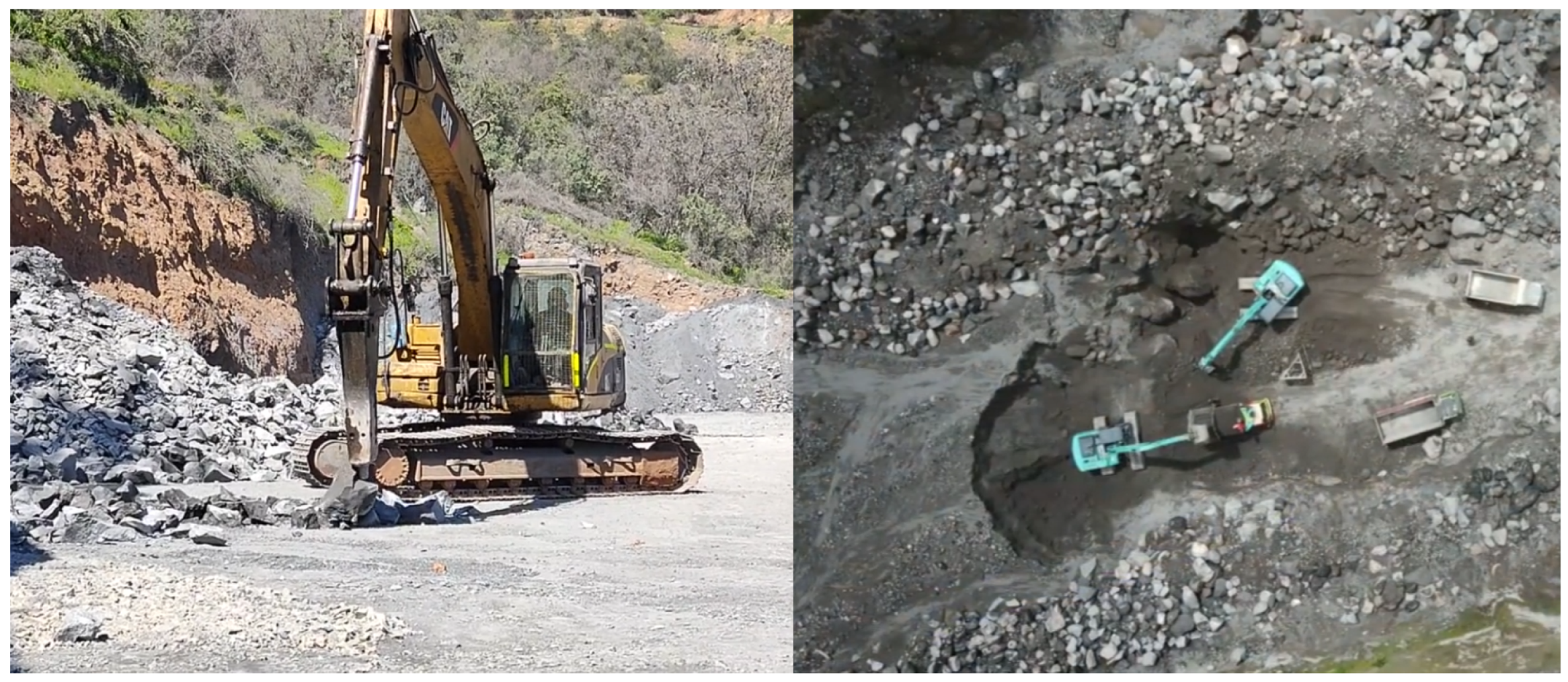Figure 1 illustrates a real surface mining comminution scenario, where the lack of geometric order, the spatial heterogeneity of the material, and the need for precise coordination between navigation and fragmentation actions are clearly evidenced.

In the domain of autonomous ground vehicles (AGVs), deep reinforcement learning methods have demonstrated strong potential for generating policies that handle nonlinear dynamics, sensory uncertainty, and stochastic scenarios. Recent surveys on autonomous driving and vehicular control [2,3], together with recent DRL architectures [4], converge on two key principles: (i) a preference for off-policy algorithms due to their sample efficiency and training stability and (ii) the careful formulation of reward functions to induce safe and high-performance policies. In this regard, Knox et al. [5] highlight that poorly designed rewards can lead to unstable policies or undesirable agent behaviors.

Studies on trajectory planning and motion planning [6,7] show that decomposing agents into behavioral subsystems accelerates learning in high-complexity tasks. Consistently, hierarchical and cooperative schemes [8], together with recent DRL surveys [2,3,9], emphasize the need for models capable of coordinating multiple objectives and operational constraints. In this context, off-policy algorithms such as Soft Actor–Critic incorporate advanced techniques—including bootstrapping, automatic entropy tuning, curriculum learning, and twin critics—that contribute to improving training stability and accelerating policy convergence [9].

The use of world models reduces the reliance on real data during training [10], which is particularly relevant in industrial mining environments where safety and operational constraints are critical [1]. Unlike structured urban environments, surface mining work areas lack well-defined roads and have limited signage, which increases the difficulty of navigation, maneuvering, target selection, and rockpile dismantling. In such scenarios, an autonomous vehicle must accurately estimate its position and orientation to operate safely; in this regard, surveys on the evolution of Simultaneous Localization and Mapping (SLAM) techniques and sensor fusion [11] establish guidelines—including the integration of DRL into their architectures [4]—to endow autonomous systems with advanced perception capabilities.

The rock pile dismantling problem is defined as a process-oriented task aimed at the controlled reduction of irregular accumulations of rocky material through the coordinated action of a mobile machine and a hydraulic manipulator. The operational objective is to transform an initially cohesive pile into a more dispersed and manageable configuration, characterized by a significant reduction in height and local material concentration, while maintaining operational safety, avoiding undesired collisions, and promoting efficient energy use.

In this context, the present work proposes a hierarchical deep reinforcement learning framework based on Soft Actor–Critic, adopting an end-to-end approach to control navigation and comminution tasks in unstructured open-pit mining scenarios. The system addresses, in an integrated manner, safe navigation, obstacle avoidance, target selection, and rock pile dismantling. The problem is modeled as a Partially Observable Markov Decision Process (POMDP), since perception—obtained from processed information derived from an overhead depth camera—is inherently limited and subject to occlusions. Consequently, the agent learns a policy based on partial observations to maximize overall process performance.

The main contributions of this work are summarized as follows:

• A hierarchical DRL framework is proposed that explicitly integrates mobile navigation and hydraulic manipulation as coupled subprocesses within a unified decision-making architecture for surface mining comminution tasks.
• A hierarchical scheme based on two specialized SAC subagents and a hysteresis-based switching mechanism is introduced, enabling stable allocation between approach, positioning, and dismantling phases, while mitigating oscillatory behaviors.
• A reward structure specific to each subagent is designed, aligned with key process performance indicators, including geometric criteria, actuator constraints, control smoothness, and energy efficiency.
• A curriculum learning scheme is incorporated to progressively increase environmental complexity during training, promoting the stability and robustness of the learned policies.
• An evaluation protocol based on multiple executions with different random seeds and confidence intervals is established, allowing consistent performance analysis and comparison of the proposed architecture with equivalent hierarchical variants and ablation studies.

The remainder of this document is organized as follows: Section 2 presents the related work; Section 3 describes the materials, the simulation environment, and the methods employed; Section 4 presents the experimental results; Section 5 discusses the obtained results; Section 6 analyzes the limitations of the study; Section 7 presents the conclusions; and finally, Section 8 outlines future research directions.

2. Related Work

In recent years, a substantial body of research has been developed in autonomous driving and mobile autonomous systems, ranging from general state-of-the-art surveys to specific approaches focused on perception, decision-making, and control. These works have significantly advanced vehicular autonomy, particularly in structured environments, and have served as the conceptual foundation for many modern deep learning and reinforcement learning architectures.

2.1. General Reviews

Zhao et al. [2] and Kuutti et al. [3] present comprehensive surveys on the use of deep learning in perception, localization, planning, and vehicular control. Complementarily, Zhao et al. [4] and Wu et al. [8] analyze recent advances in DRL applied to autonomous vehicles, highlighting practical applications and open challenges. Consistently, these surveys converge on a preference for off-policy algorithms—such as DQN, DDPG, SAC, and TD3—due to their sample efficiency and stability in stochastic and high-complexity environments. Other studies, such as those by Haydari et al. [12] and Aradi [7], review DRL applications in Intelligent Transportation Systems, including trajectory planning.

However, most of these surveys focus on structured or semi-structured scenarios and do not explicitly address coordination between navigation and manipulation, nor the formulation of tasks for complex industrial processes under partial observability and severe operational constraints, as in open-pit mining.

2.2. Perception and Sensor Fusion

Environmental perception and sensor fusion constitute fundamental components of autonomous systems. Numerous studies have explored multimodal architectures that combine cameras and LiDAR to generate three-dimensional representations of the environment, either through bird’s-eye view (BEV) representations integrated with DRL [13] or through 3D semantic segmentation based on the fusion of visual and depth data [14]. In industrial applications, perception systems oriented toward specific rock fragmentation tasks have also been proposed [15]. Additional studies analyze the impact of adverse operating conditions [16] and the vulnerabilities of vision-only systems [17].

However, a large portion of these approaches focuses on improving perceptual accuracy without explicitly integrating limited perception into hierarchical decision-making frameworks oriented toward complex industrial processes, such as those required in mining comminution.

2.3. Decision-Making, Safety, and Reward Design

In autonomous decision-making, safety and proper reward design are critical factors. Knox et al. [5] analyze the risks associated with poorly defined rewards in autonomous driving. To mitigate these issues, Safe Reinforcement Learning approaches with explicit constraints have been proposed [18], as well as hybrid methods that combine DRL with Monte Carlo Tree Search [19]. Other works explore frameworks based on game theory or Inverse Reinforcement Learning; Lee et al. [20] propose policies that execute contingency actions in response to unexpected failures.

However, these studies primarily focus on structured environments or on the enforcement of explicit constraints, without directly addressing the design of process-oriented reward functions for complex industrial applications, where safety, energy efficiency, and control stability must be simultaneously balanced under partial observability.

2.4. Trajectory Planning

Mir et al. [6] present a comprehensive review of trajectory planning techniques, covering classical methods—such as RRT* and lattice planning—as well as modern DRL-based approaches. Aradi [7] analyzes motion planning as a sequential decision-making problem in dynamic environments. Along this line, Lee and Yusuf [21] demonstrate that autonomous navigation can be addressed through implicit DRL-based planning without explicit maps, integrating perception and decision-making in an end-to-end scheme.

Other works integrate different learning paradigms, such as the combination of RL and Deep Inverse Reinforcement Learning (You et al. [22]), or address safe planning under uncertainty through integrated mapping and planning frameworks [23] or route generation in mobile robotic systems operating under dense traffic conditions [24]. More recently, DRL-based trajectory planning approaches have been proposed for heavy machinery and unstructured construction environments, demonstrating the feasibility of RL for continuous planning tasks under complex physical constraints [25]. In multi-agent contexts, hybrid DRL methods are employed for coordination and traffic flow optimization [26,27].

However, these contributions typically treat planning as a problem decoupled from continuous control and physical interaction with the environment. In contrast, mining comminution operations require tight coordination between navigation and physical interaction with heterogeneous rocky material, under operational constraints and partial observability.

2.5. Low-Level Control

Low-level control in autonomous vehicles has been extensively studied. De Morais et al. [28] propose a robust vision-based DRL framework for lane keeping and obstacle avoidance. In contrast, Wang et al. [29] apply RL to velocity control in car-following scenarios. Liu et al. [30] integrate LQR control with Soft Actor–Critic for reverse maneuvers in confined spaces.

In the domain of electrohydraulic systems, Rout and Kumawat [31] employ RL with Lyapunov-based stability guarantees for position tracking in proportional valves, while Cao et al. [32] apply RL to continuous control tuning in heavy tunnel boring machinery, demonstrating improvements in stability and efficiency compared to traditional empirical strategies. Likewise, Leng et al. [33] introduce the TD3 algorithm for controlling critical parking maneuvers in autonomous vehicles, showing that DRL can robustly handle highly nonlinear and saturated dynamics in continuous control tasks. Other hybrid approaches include the use of Deep Deterministic Policy Gradient (DDPG) with explainable techniques [34], adaptive control in underwater vehicles [35], and recent extensions of the actor–critic framework that improve learning stability [36,37].

However, these works focus on individual subsystems and do not explicitly consider the coordination between low-level control, behavioral planning, and the execution of complex physical tasks, such as those required in mining comminution processes.

2.6. World Models and Transfer Learning

To reduce the sim-to-real gap, several studies integrate world models and transfer learning. Matsuo et al. [10] highlight the use of generative models to learn environment dynamics, while Hieu et al. [38] propose transferable frameworks for autonomous vehicles under adverse conditions. More recently, Cui et al. [39] introduce event-triggered attention mechanisms to improve the stability of end-to-end agents. Additionally, Ampuero et al. [40] demonstrate the feasibility of waypoint-based navigation using DRL with a minimal sensor set, validating sim-to-real transfer in unstructured terrains such as beaches.

While these approaches help reduce the sim-to-real gap, their direct application in complex industrial environments often requires highly detailed models and additional training. In mining, where physical testing is costly and risky, it is therefore relevant to evaluate robust policies in simulation while explicitly acknowledging model limitations, as a foundation for future real-world transfer strategies.

2.7. Industrial and Mining Machinery

In the domain of heavy machinery, various solutions have been developed to automate industrial tasks. Lampinen et al. [41] and Samtani et al. [42] address rock fragmentation using stationary machinery based on three-dimensional perception and DRL. Cárdenas et al. [43,44] extend these approaches to Load–Haul–Dump vehicles in underground mining. In mining perception, Huang et al. [45] and Rodríguez-Guillén et al. [46] propose rock detection methods for visually complex environments, while Ismael et al. [47] analyze the performance of hydraulic breakers as a function of rock mass properties. In related applications, You et al. [48] apply imitation learning to autonomous bulldozers. In hydraulic machinery, Kim et al. [49] integrate model-based control and RL to optimize velocity tracking in semi-automated excavators. A general study on heavy machinery automation is presented by Machado et al. [50].

However, most of these contributions focus on stationary machinery, specific tasks, or highly controlled environments, and do not explicitly address the hierarchical coordination between mobile navigation and hydraulic manipulation in unstructured mining scenarios. The automation of rock pile dismantling in surface mining requires integrating imperfect perception, hierarchical decision-making, and continuous control under process-specific operational constraints, which motivates the approach proposed in this work.

3. Materials and Methods

All simulations, training, and evaluations of the proposed framework were conducted on a desktop computer equipped with an Intel Core i9-12900KF processor (Intel Corporation, Santa Clara, CA, USA), 64 GB of DDR4 RAM, and an NVIDIA GeForce RTX 3090 graphics card with 24 GB of memory (NVIDIA Corporation, Santa Clara, CA, USA), running 64-bit Windows 11 (Microsoft Corporation, Redmond, WA, USA). The reported results were obtained using MATLAB R2024b (The MathWorks, Inc., Natick, MA, USA), together with Simulink R2024b and the Reinforcement Learning Toolbox R2024b (The MathWorks, Inc., Natick, MA, USA), ensuring consistency across the training, evaluation, and analysis stages of the SAC-1 and SAC-2 subagents. Agent configurations—including network architectures, state and action spaces, reward functions, and automatic entropy tuning—were kept constant throughout the experiment to ensure validity and reproducibility.

3.1. Problem Formulation

The proposed framework corresponds to a hierarchical deep reinforcement learning agent based on Soft Actor–Critic, with an end-to-end design and the incorporation of twin critics, automatic entropy tuning, and curriculum learning. The hierarchical formulation decomposes the overall surface mobile comminution task into coupled subprocesses that coordinate navigation and hydraulic manipulation.

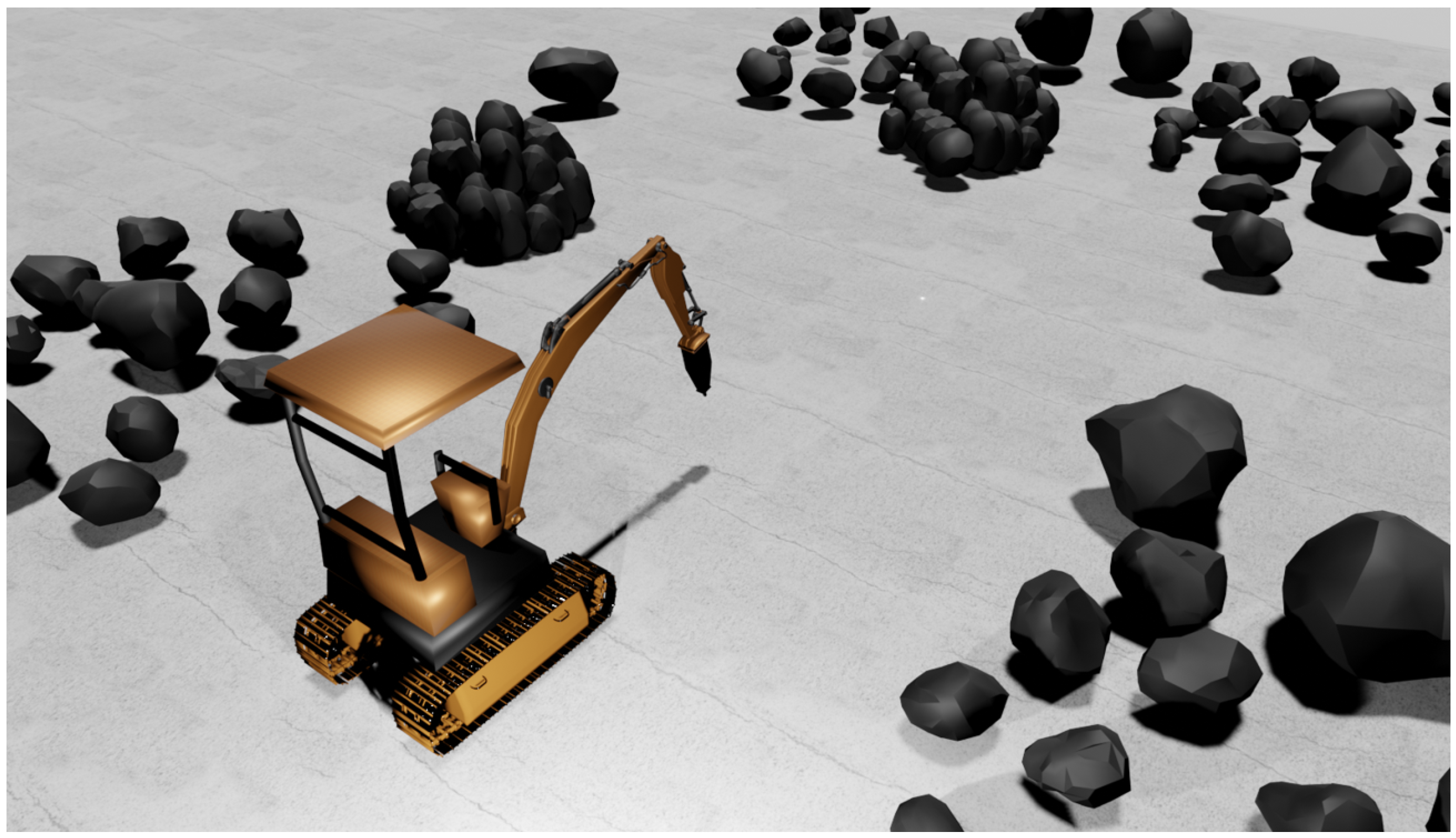
The system is modeled as a Partially Observable Markov Decision Process (POMDP) due to the incomplete information provided by an overhead depth camera (Figure 2). In this context, the agent must operate in unstructured environments, with perceptual uncertainty and nonlinear dynamics. Under this formulation, the objective is to learn robust policies that enable safe and efficient operation based on partial observations of the environment.

The hierarchical agent is composed of two specialized subagents, associated with distinct operational stages:

1.

Navigation subagent (SAC-1), responsible for autonomous locomotion, obstacle avoidance, and safe approach toward the target rock pile;

2.

Manipulation subagent (SAC-2), responsible for dismantling the rock pile through continuous control of the hydraulic manipulator.

Coordination is achieved through a temporal switching mechanism $\kappa \left(t\right)$, which activates SAC-2 and deactivates SAC-1 when the distance to the pile satisfies $d_t\le d_{\mathrm{thr}}$. To avoid spurious switching and oscillatory behavior near the threshold, the mechanism incorporates hysteresis, ensuring stable transitions between the approach, positioning, and dismantling phases.

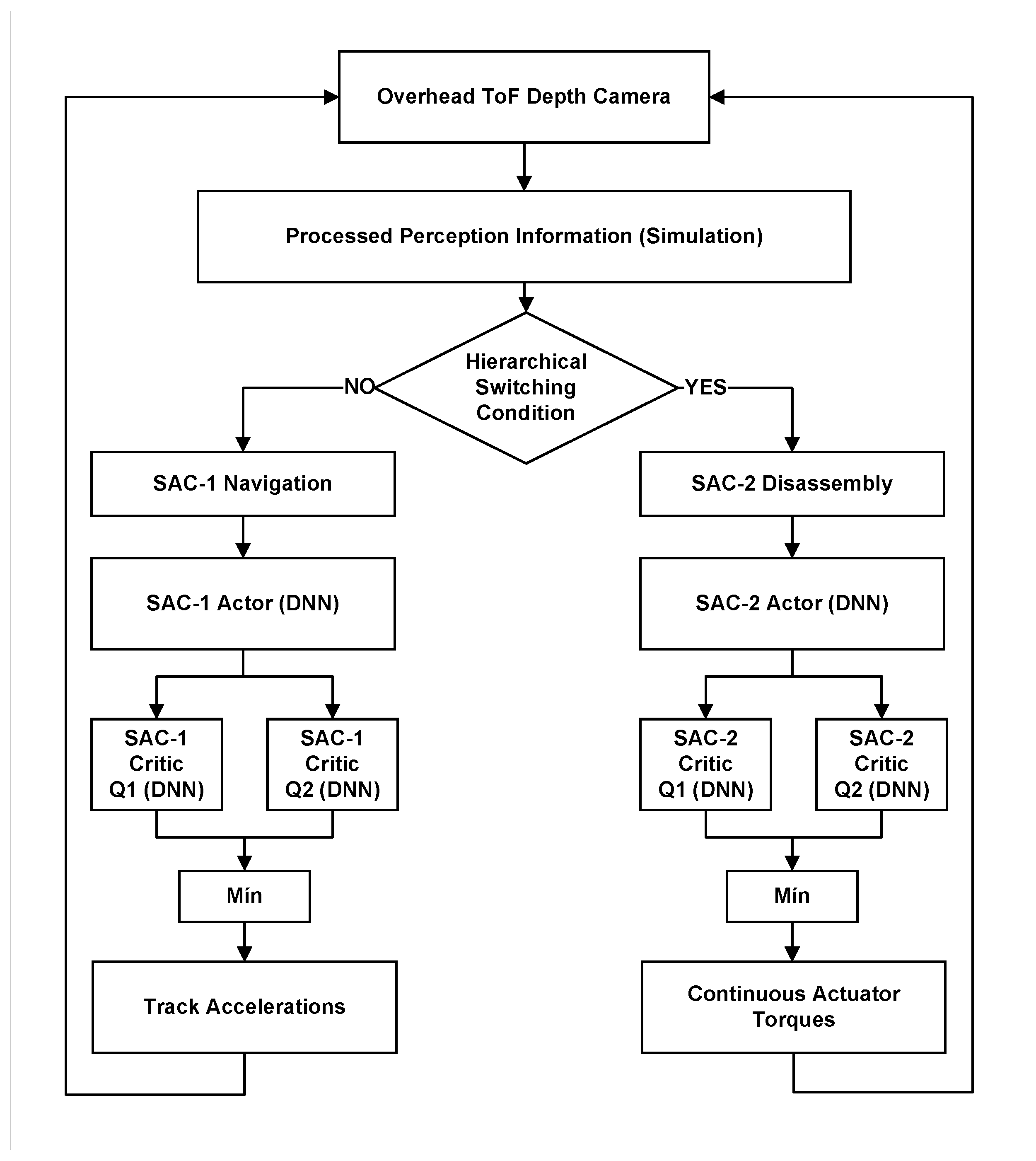
This scheme is illustrated in Figure 3 and formalized in Equation (1). Although the switching criterion is based on a simple and directly observable geometric metric, this choice is justified by its robustness and operational traceability in unstructured environments. The incorporation of alternative criteria—such as perceptual confidence metrics, geometric descriptors of the rock pile, or value-based arbitration—is considered a natural extension and is discussed as a direction for future research.

$$\kappa \left(t\right)=\left\{\begin{array}{cc}SAC-1,\hfill & \mathrm{if}{d}_t>d_{\mathrm{thr}},\hfill \\ SAC-2,\hfill & \mathrm{if}{d}_t\le d_{\mathrm{thr}},\hfill \end{array}\right.$$

(1)

The agent is formulated as a Partially Observable Markov Decision Process, represented by the tuple $\langle \mathcal{S},\mathcal{A},\mathcal{T},\mathcal{R},\Omega ,\mathcal{O},\gamma \rangle$, where $\mathcal{S}$ denotes the state space, $\mathcal{A}$ the action space, $\mathcal{T}$ the state transition dynamics, $\mathcal{R}$ the reward function, $\Omega$ the observation space, $\mathcal{O}$ the observation function, and $\gamma \in (0,1)$ the discount factor.

3.1.1. State Space $\mathcal{S}$

The system state at time t, denoted as $s_t\in \mathcal{S}$, describes the internal configuration of the environment and the machinery and includes the following:

(i)

the state of the mobile machinery $\mathrm{M}$, defined by its planar position and orientation $(x^{\mathrm{M}},y^{\mathrm{M}},{\theta }^{\mathrm{M}})$, together with its linear and angular velocities;

(ii)

the state of the hydraulic manipulator, characterized by the joint positions $q_1,\dots ,q_4$;

(iii)

the representation of the comminution terrain, composed of the positions and heights of individual rocks and rock piles modeled as ${\left\{(x_i^{\mathrm{R}},y_i^{\mathrm{R}},z_i^{\mathrm{R}})\right\}}_{i=1}^N$. Each rock or cluster ($\mathrm{R}$) is approximated by a cuboid or an enclosing polyhedron obtained from the segmentation of the point cloud captured by the overhead depth camera.

3.1.2. Observation Space $\Omega$ and Observation Function $\mathcal{O}$

The observation space $\Omega$ is defined based on the information obtained from an overhead depth camera. The observation function $\mathcal{O}:\mathcal{S}\to \Omega$ models the mapping from the true state $s_t$ to a partial observation $o_t=\mathcal{O}\left(s_t\right)$, reflecting the partially observable nature of the environment.

Each observation $o_t$ is constructed from the processing of the 3D point cloud captured by the camera, through segmentation and detection stages of enclosing polyhedra (bounding boxes) representing individual rocks and rock piles. These processed perceptual variables are used as inputs to the subagents during both training and policy execution.

In simulation, $\mathcal{O}$ directly provides these processed variables, without explicitly modeling sensor noise, occlusions, segmentation errors, or latencies. This perceptual abstraction constitutes a methodological decision aimed at isolating the performance of the hierarchical scheme and the reinforcement learning algorithm under idealized perceptual conditions. Nevertheless, perceptual uncertainty may degrade performance in real deployments; therefore, incorporating noise, partial occlusions, and domain randomization techniques is considered a natural extension and is addressed as future work.

3.1.3. Transition Function $\mathcal{T}$

The transition function $\mathcal{T}(s,a,s^{\prime })$ defines the probability of transitioning from a state $s\in \mathcal{S}$ to the next state $s^{\prime }\in \mathcal{S}$ after executing an action $a\in \mathcal{A}$. Given the complexity of the system, $\mathcal{T}$ is not specified analytically and is implicitly embedded within the simulation environment.

In particular, the simulator applies the equations of motion of the mobile machinery and models physical interactions with individual rocks (obstacles) and rock piles (targets), generating the next state through an implicit dynamics of the form $s^{\prime }=f(s,a)$. This approach is consistent with model-free methods, where the agent estimates the dynamics from experience samples obtained through direct interaction with the environment [42].

3.1.4. Reward Function $\mathcal{R}$

The reward function $\mathcal{R}(s,a)$ guides the agent toward the efficient execution of mobile comminution tasks. To this end, a shaped reward with multiple terms is employed, designed to balance incentives for desired behaviors and penalties for undesired actions.

In order to balance immediate and long-term rewards, a discount factor $\gamma \in (0,1)$ close to $0.99$ is used, in accordance with recent DRL literature [2,3,7]. This formulation allows the agent to learn an optimal policy ${\pi }^{*}$ under the maximum entropy principle, as defined in Equation (2).

$${\mathcal{J}}_{\mathrm{SAC}}\left(\pi \right)={\mathbb{E}}_{{\rho }_{\pi }}\left[\sum _{t=0}^{\infty }{\gamma }^t\left(r(s_t,a_t)-\alpha log\pi (a_t\mid s_t)\right)\right],$$

(2)

where $\alpha$ is the entropy coefficient that regulates the trade-off between exploration and exploitation; $\gamma$ is the discount factor; and $\pi$ denotes the stochastic policy of the agent.

Since the agent receives partial observations of the environment, the problem is modeled as a POMDP. In practice, to maintain consistency with the standard formulation of the SAC algorithm, the notation $s_t$ is adopted to represent the observation vector $o_t$ effectively provided to the policy $\pi (a_t\mid o_t)$ and to the critics, even though, in a strict sense, $o_t\ne s_t$.

3.2. Hierarchical SAC Agent Architecture

3.2.1. SAC-1 Subagent: Navigation

The SAC-1 subagent controls the autonomous navigation of the tracked machinery, enabling safe locomotion, collision avoidance with individual rocks, and a progressive approach toward the target pile. It operates on a global observational representation suitable for planning in unstructured mining scenarios.

The observation vector of the navigation subagent is denoted by $o_t^{\left(1\right)}$ and integrates perceptual information from the environment and the kinematic state of the machine, as expressed in Equation (3):

$$o_t^{\left(1\right)}=\left({\mathbf{R}}_t,{\mathbf{p}}_t,{\mathbf{M}}_t\right),$$

(3)

where ${\mathbf{R}}_t\in {\mathbb{R}}^{3N_t}$ corresponds to the vector that groups the spatial coordinates $(x_i^{\mathrm{R}},y_i^{\mathrm{R}},z_i^{\mathrm{R}})$ of individual rocks and rock piles detected in the environment at time t.

The term $N_t$ denotes the total number of objects (rocks or rock clusters) identified in the scene at time t. These coordinates are obtained from cuboids or enclosing polyhedra derived from the segmentation of the point cloud captured by the overhead camera. In matrix form, $R_t$ is expressed as follows:

$${\mathbf{R}}_t={\left[\begin{array}{ccc}{x}_{1,t}& \cdots & x_{N_t,t}\\ y_{1,t}& \cdots & y_{N_t,t}\\ z_{1,t}& \cdots & z_{N_t,t}\end{array}\right]}^{\top },$$

The vector ${\mathbf{p}}_t=(x_t^{\mathrm{M}},y_t^{\mathrm{M}},{\theta }_t^{\mathrm{M}})$ represents the global pose of the machinery, and ${\mathbf{M}}_t\in {\mathbb{R}}^{H\times W}$ corresponds to a two-dimensional map encoding terrain occupancy and relative elevation.

The continuous action space $a^{\left(1\right)}\in {\mathcal{A}}^{\left(1\right)}$ corresponds to normalized differential accelerations of the left and right tracks, enabling forward motion, turning, or braking. Under the action $a_t^{\left(1\right)}=(a_L,a_R)$, differential-drive kinematics govern the evolution of the pose within the simulated environment.

The reward of the SAC-1 subagent (Equation (4)) integrates terms that reduce the Euclidean distance to the target to encourage alignment, minimize oscillations and abrupt maneuvers, penalize proximity to obstacles, and regulate control effort and smoothness, thereby promoting safe and efficient navigation:

$$\begin{array}{cc}\hfill r_t^{\left(1\right)}& =R_g{\mathbf{1}}_{\mathrm{goal}}-R_c{\mathbf{1}}_{\mathrm{col}}+w_d\Delta d_t+w_g{e}^{-d_t^2/{\sigma }_d^2}\hfill \\ \hfill & + w_{\theta }cos{\theta }_t+w_v{v}_{t}cos{\theta }_t-w_o\sum _j{e}^{-d_{j,t}^2/{\rho }^2}{\mathbf{1}}_j\hfill \\ \hfill & -w_a{\parallel u_t\parallel }_2^2-w_j{\parallel u_t-{\tilde{u}}_t\parallel }_2^2,\hfill \end{array}$$

(4)

where

• $u_t=a_t^{\left(1\right)}=(a_{L,t},a_{R,t})$ and ${\tilde{u}}_t=a_{t-1}^{\left(1\right)}$ represent, respectively, the current and previous differential accelerations applied to the left and right tracks.
• $R_g$ is the positive terminal reward granted when the agent successfully reaches the target rock pile, activated by the indicator ${\mathbf{1}}_{\mathrm{goal}}={\mathbf{1}}_{\{d_t<{\epsilon }_d\wedge |{\theta }_t|<{\epsilon }_{\theta }\}}$, where ${\epsilon }_d$ and ${\epsilon }_{\theta }$ correspond to distance and angular alignment thresholds, respectively.
• $R_c$ denotes the penalty applied upon collision with an obstacle, activated by the indicator ${\mathbf{1}}_{\mathrm{col}}$.
• $\Delta d_t=d_{t-1}-\gamma d_t$ represents the discrete progress toward the target, incorporating the discount factor $\gamma$. This term implements a potential-based shaping scheme, equivalent to $r^{\prime }=r+\gamma \Phi \left(s_{t+1}\right)-\Phi \left(s_t\right)$, with $\Phi \left(s\right)=-d\left(s\right)$, which preserves optimal policy invariance.
• The Gaussian term $w_g{e}^{-d_t^2/{\sigma }_d^2}$ smoothly and boundedly rewards proximity to the target, where ${\sigma }_d$ controls the spatial extent of the reward field.
• $w_{\theta }cos{\theta }_t$ rewards alignment between the machinery orientation and the direction toward the target, where ${\theta }_t$ denotes the angular error with respect to the vector connecting the current position to the target rock pile.
• $w_v{v}_{t}cos{\theta }_t$ promotes effective motion toward the target by rewarding the component of the linear velocity $v_t$ projected along the target direction, implicitly penalizing lateral or opposing movements.
• The repulsion term $w_o{\sum }_j{e}^{-d_{j,t}^2/{\rho }^2}{\mathbf{1}}_j$ penalizes proximity to obstacles, where $d_{j,t}$ is the distance to obstacle j, $\rho$ controls the decay radius of the penalty, and ${\mathbf{1}}_j={\mathbf{1}}_{\{d_{j,t}<d_{\mathrm{safe}}\}}$ activates the penalty only when a minimum safety distance $d_{\mathrm{safe}}$ is violated.
• $w_a{\parallel u_t\parallel }_2^2$ penalizes control effort (large track accelerations), favoring energy-efficient actions and avoiding unnecessary actuator saturation.
• $w_j{\parallel u_t-{\tilde{u}}_t\parallel }_2^2$ penalizes abrupt changes between consecutive actions, promoting temporal smoothness in control and contributing to the dynamic stability of the vehicle.

Although the SAC-1 reward function includes multiple terms, each component fulfills a differentiated functional role associated with progress, geometric alignment, safety, and control smoothness. To avoid redundancy and promote learning stability, the reward weights were empirically tuned to comparable scales. A detailed sensitivity analysis and exhaustive per-component ablation studies are considered beyond the scope of this work and are identified as directions for future research.

3.2.2. SAC-2 Subagent: Manipulation

The SAC-2 subagent is activated by $\kappa \left(t\right)$ when the machine reaches the vicinity of a target rock pile ($d_t\le d_{\mathrm{thr}}$). At this stage, SAC-2 controls the hydraulic arm to apply impacts that reduce the pile height and promote its dismantling into individual rocks.

The observation of the manipulation subagent, denoted as $o_t^{\left(2\right)}$, integrates the geometry of the rock pile and the joint configuration of the arm. The pile is represented through the coordinates of its detected components, while the manipulator state is described by ${\mathbf{q}}_t={(q_{1,t},q_{2,t},q_{3,t},q_{4,t})}^{\top }$, as formalized in Equation (5):

$$\begin{array}{cc}\hfill o_t^{\left(2\right)}& =\left({\mathbf{R}}_t^{\mathrm{pile}},{\mathbf{q}}_t\right),\hfill \\ \hfill {\mathbf{R}}_t^{\mathrm{pile}}& =\left[\begin{array}{ccc}{x}_{1,t}& \cdots & x_{N_t,t}\\ y_{1,t}& \cdots & y_{N_t,t}\\ z_{1,t}& \cdots & z_{N_t,t}\end{array}\right]\in {\mathbb{R}}^{3\times N_t},{\mathbf{q}}_t={\left[\begin{array}{cccc}{q}_{1,t}& q_{2,t}& q_{3,t}& q_{4,t}\end{array}\right]}^{\top }\in {\mathbb{R}}^4,\hfill \end{array}$$

(5)

where

• $o_t^{\left(2\right)}$ corresponds to the observation vector of the manipulation subagent (SAC-2), which is activated when the mobile base reaches the operational region of the target rock pile.
• ${\mathbf{R}}_t^{\mathrm{pile}}\in {\mathbb{R}}^{3\times N_t}$ contains the spatial coordinates $(x_{i,t},y_{i,t},z_{i,t})$ of the $N_t$ detected rock components that constitute the pile at time t.
• ${\mathbf{q}}_t={(q_{1,t},q_{2,t},q_{3,t},q_{4,t})}^{\top }$ is the vector of joint positions of the hydraulic arm that manipulates the impact hammer.
• Each variable $q_{k,t}$ represents the state of the k-th degree of freedom of the manipulator, ordered from the base to the end-effector.
• The rock coordinates are expressed in a normalized local reference frame with respect to the pile centroid, with the aim of improving the translational invariance of the learned policy.
• The number of components $N_t$ varies throughout the episode, reflecting the progressive fragmentation process.

The action space of SAC-2, $a^{\left(2\right)}$, corresponds to continuous torque commands. Although the full mechanical model includes four joint torques, in the reported experiments, SAC-2 actively controls only two dominant joints, with the remaining joints held at predefined fixed configurations to ensure feasibility and stability. This reduction decreases learning complexity and allows isolating the hierarchical scheme’s performance in the manipulation task, without significantly altering the relevant impact dynamics.

The reward function of SAC-2 (Equation (6)) combines terms that reduce pile height, encourage effective impacts, and penalize excessive torques and abrupt changes, thereby promoting smooth and efficient actuation.

$$r_t^{\left(2\right)}=w_h(h_{t-1}-h_t)+w_c{C}_t-w_{\tau }{\parallel a_t^{\left(2\right)}\parallel }_2^2-w_j{\parallel a_t^{\left(2\right)}-a_{t-1}^{\left(2\right)}\parallel }_2^2.$$

(6)

where

• $r_t^{\left(2\right)}$ corresponds to the instantaneous reward provided to SAC-2 at time step t.
• $h_t$ represents the average height of the rock pile, computed from the three-dimensional coordinates of the detected rock components. The term $(h_{t-1}-h_t)$ measures the instantaneous height reduction between two consecutive time steps and constitutes a potential-based shaping term of the form $r^{\prime }=r+\gamma \Phi \left(s_{t+1}\right)-\Phi \left(s_t\right)$, with $\Phi \left(h\right)=h$, which preserves optimal policy invariance.
• $C_t\in \{0,1\}$ is an effective contact indicator, which is activated ($C_t=1$) when the hydraulic hammer or arm produces an impact on the pile; otherwise, $C_t=0$.
• $a_t^{\left(2\right)}={({\tau }_{1,t},{\tau }_{2,t},{\tau }_{3,t},{\tau }_{4,t})}^{\top }$ is the vector of continuous torques applied to the degrees of freedom of the hydraulic arm at time step t, while $a_{t-1}^{\left(2\right)}$ corresponds to the command applied at the previous time step.
• The term ${\parallel a_t^{\left(2\right)}\parallel }_2^2$ penalizes the magnitude of the control effort, avoiding actuator saturation and excessive energy consumption.
• The term ${\parallel a_t^{\left(2\right)}-a_{t-1}^{\left(2\right)}\parallel }_2^2$ penalizes abrupt variations between consecutive commands, enforcing temporal smoothness in the actuation and reducing mechanical stress on the hydraulic system.
• The coefficients $w_h$, $w_c$, $w_{\tau }$, and $w_j$ are empirically tuned weights used to balance height reduction, impact effectiveness, and control smoothness.

Similar to SAC-1, the reward weights were empirically tuned to comparable scales to avoid dominance by any single term and promote training stability. A component-wise sensitivity analysis is considered as future work.

3.3. Learning Algorithm

To address the complexity of the problem, the system is implemented as a hierarchical architecture (Figure 3) with a switching mechanism that decomposes the operation into two subtasks: (i) autonomous navigation toward the target rock pile while avoiding collisions (SAC-1) and (ii) pile dismantling through hydraulic arm control (SAC-2).

The switching mechanism $\kappa \left(t\right)$ regulates the activation of the subagents based on the distance $d\left(t\right)$ to the target pile. When $d\left(t\right)$ falls below the threshold $d_{\mathrm{thr}}$, SAC-1 is deactivated, and SAC-2 is activated. To prevent frequent switching and oscillatory behavior between operational modes, hysteresis is incorporated through an additional exit threshold, as detailed in Algorithm 1.

Algorithm 1 Hierarchical SAC agent with hysteresis for switching between SAC-1 (navigation) and SAC-2 (manipulation)

1: Input: Policies ${\pi }_{{\varphi }_1}$ (SAC-1, navigation) and ${\pi }_{{\varphi }_2}$ (SAC-2, manipulation); hysteresis thresholds $d_{\mathrm{thr}}^{\mathrm{in}}<d_{\mathrm{thr}}^{\mathrm{out}}$; height termination threshold $h_{\mathrm{thr}}$; horizon T.   2: Initialize: mode ←Nav; $t\leftarrow 0$.   3: while  $t<T$ do   4:    Acquire observations $o_t^{\left(1\right)}$ (navigation) and $o_t^{\left(2\right)}$ (pile + arm).   5:    Estimate distance to the target pile $d_t$ and pile height $h_t$.   6:    if mode = Nav and $d_t\le d_{\mathrm{thr}}^{\mathrm{in}}$ then    7:        mode ← Manip {deactivate SAC-1 and activate SAC-2}   8:    else if mode = Manip and $d_t\ge d_{\mathrm{thr}}^{\mathrm{out}}$ then    9:        mode ← Nav {reactivate SAC-1 and deactivate SAC-2} 10:    end if 11:    Switching mechanism $\kappa \left(t\right)$: 12:           $\kappa \left(t\right)=1$ if mode =Nav,    $\kappa \left(t\right)=2$ if mode = Manip. 13:    if mode = Nav then 14:        $a_t^{\left(1\right)}\leftarrow {\pi }_{{\varphi }_1}\left(o_t^{\left(1\right)}\right)$ {differential track accelerations} 15:        Apply $a_t^{\left(1\right)}$ to the mobile base. 16:    else 17:        $a_t^{\left(2\right)}\leftarrow {\pi }_{{\varphi }_2}\left(o_t^{\left(2\right)}\right)$ {joint torques} 18:        Apply $a_t^{\left(2\right)}$ to the hydraulic arm. 19:    end if 20:    if $h_t\le h_{\mathrm{thr}}$ then 21:        terminate {pile dismantled} 22:    end if 23:    $t\leftarrow t+1$ 24: end while

The SAC-1 subagent guides the mobile base from its initial position to the vicinity of the target rock pile. The observation $o_t^{\left(1\right)}$ combines the global pose of the vehicle with spatial information about the detected rock elements. Differential accelerations of the tracks define the action space, and the reward function promotes progress toward the target, alignment, obstacle avoidance, and smooth control.

As detailed in Algorithm 2, SAC-1 training incorporates twin critics, automatic entropy coefficient tuning, and curriculum learning to increase the environment’s complexity gradually. This design enhances learning stability and enables the acquisition of robust policies that reliably reach the operational region required to activate SAC-2.

Algorithm 2 Training of the SAC-1 subagent (Navigation)

1: Input: discount factor $\gamma$, minibatch size B, warm-up steps $N_{\mathrm{warm}}$, learning rates ${\eta }_Q$, ${\eta }_{\pi }$, ${\eta }_{\alpha }$, target update rate ${\tau }_{\mathrm{tgt}}$, target entropy $H_{\mathrm{tgt}}$, number of episodes $M_1$, horizon $T_1$.   2: Initialize actor policy ${\pi }_{{\varphi }_1}$, critics $Q_{{\theta }_1},Q_{{\theta }_2}$, and target networks ${\theta }_i^{\prime }\leftarrow {\theta }_i$.   3: Initialize entropy coefficient $\alpha$ and replay buffer ${\mathcal{D}}_1$.   4: for episode $=1$ to $M_1$ do   5:    Set environment difficulty using SampleCurriculum$\left(\mathrm{episode}\right)$.   6:    $s_0\leftarrow \mathrm{resetEnv}\left(\right)$;   $o_0^{\left(1\right)}\leftarrow \mathcal{O}\left(s_0\right)$.   7:    for $t=0$ to $T_1-1$ do   8:       if $|{\mathcal{D}}_1| < N_{\mathrm{warm}}$ then   9:          $a_t^{\left(1\right)}\sim \mathcal{U}(-1,1)$ 10:       else 11:          $a_t^{\left(1\right)}\sim {\pi }_{{\varphi }_1}(·\mid o_t^{\left(1\right)})$ 12:       end if 13:       Execute $a_t^{\left(1\right)}$; receive $(r_t^{\left(1\right)},s_{t+1},d_t)$. 14:       Store $(s_t,a_t^{\left(1\right)},r_t^{\left(1\right)},s_{t+1},d_t)$ in ${\mathcal{D}}_1$. 15:       Sample minibatch $\mathcal{B}\subset {\mathcal{D}}_1$ of size B. 16:       for each $(s,a,r,s^{\prime },d)\in \mathcal{B}$ do 17:          $o^{\prime \left(1\right)}\leftarrow \mathcal{O}\left(s^{\prime }\right)$;   sample $a^{\prime }\sim {\pi }_{{\varphi }_1}(·|o^{\prime \left(1\right)})$. 18:          $\ell \leftarrow log{\pi }_{{\varphi }_1}\left(a^{\prime }\right|o^{\prime \left(1\right)})$. 19:          $y\leftarrow r+(1-d)\gamma \left(min\{Q_{{\theta }_1^{\prime }}(s^{\prime },a^{\prime }),Q_{{\theta }_2^{\prime }}(s^{\prime },a^{\prime })\}-\alpha \ell \right)$. 20:          Update critics: ${\theta }_i\leftarrow {\theta }_i-{\eta }_Q\nabla {(Q_{{\theta }_i}(s,a)-y)}^2$, $i\in \{1,2\}$. 21:      end for 22:      Sample $a\sim {\pi }_{{\varphi }_1}(·|o_t^{\left(1\right)})$;   $\ell \leftarrow log{\pi }_{{\varphi }_1}\left(a\right|o_t^{\left(1\right)})$. 23:      Update actor: ${\varphi }_1\leftarrow {\varphi }_1-{\eta }_{\pi }\nabla (\alpha \ell -Q_{{\theta }_1}(s_t,a))$. 24:      Update entropy: $\alpha \leftarrow \alpha -{\eta }_{\alpha }\nabla \left[\alpha (-\ell -H_{\mathrm{tgt}})\right]$. 25:      Update target networks: ${\theta }_i^{\prime }\leftarrow {\tau }_{\mathrm{tgt}}{\theta }_i+(1-{\tau }_{\mathrm{tgt}}){\theta }_i^{\prime }$. 26:      $s_t\leftarrow s_{t+1}$;   $o_{t+1}^{\left(1\right)}\leftarrow \mathcal{O}\left(s_{t+1}\right)$. 27:      if $d_t=1$ then 28:         break 29:      end if 30:    end for 31: end for

where

• ${\pi }_{{\varphi }_1}$ denotes the Gaussian stochastic policy (actor) of SAC-1 parameterized by ${\varphi }_1$.
• $Q_{{\theta }_1}$ and $Q_{{\theta }_2}$ correspond to the twin critics employed to mitigate Q-value overestimation.
• $\alpha$ is the temperature coefficient that regulates the entropy term, enabling a balance between exploration and exploitation.
• The smoothed Bellman target value y is given by Equation (7):

  $$y=r+(1-d)\gamma \left[\underset{i}{min}{Q}_{{\theta }_i^{\prime }}(s^{\prime },a^{\prime })-\alpha log{\pi }_{{\varphi }_1}\left(a^{\prime }\right|o^{\prime \left(1\right)})\right].$$

  (7)
• The actor parameters ${\varphi }_1$ are optimized by minimizing Equation (8):

  $$J_{\pi }={\mathbb{E}}_{a\sim \pi }\left[\alpha log{\pi }_{{\varphi }_1}\left(a\right|o^{\left(1\right)})-Q_{{\theta }_1}(s,a)\right].$$

  (8)
• The target entropy coefficient $H_{\mathrm{tgt}}$ defines the desired exploration level, while ${\tau }_{\mathrm{tgt}}$ corresponds to the Polyak averaging factor used for the soft update of the target networks.
• The replay buffer ${\mathcal{D}}_1$ stores approximately $6\times {10}^6$ transitions. Large minibatches ($B=1024$) are employed to reduce gradient variance, preceded by an initial warm-up phase of $5\times {10}^4$ random steps.

During SAC-1 training, the critics have access to the complete simulator state $s_t$, while the actor operates exclusively on partial observations $o_t^{\left(1\right)}$. This strategy follows a centralized training, decentralized execution (CTDE) paradigm, which helps stabilize learning without increasing perceptual requirements during execution.

When the agent enters the operational region, $\kappa \left(t\right)$ activates SAC-2. The observation $o_t^{\left(2\right)}$ provides local geometric information of the rock pile along with the joint state of the hydraulic arm. The action space consists of joint torque commands, and the reward function prioritizes reducing pile height and increasing effective contacts, while penalizing excessive effort and abrupt changes in action. The training procedure of SAC-2 is presented in Algorithm 3.

Algorithm 3 Training of the SAC-2 subagent (Manipulation)

1: Input: discount factor $\gamma$, minibatch size B, warm-up steps $N_{\mathrm{warm}}$, learning rates ${\eta }_Q$, ${\eta }_{\pi }$, ${\eta }_{\alpha }$, target update rate ${\tau }_{\mathrm{tgt}}$, target entropy $H_{\mathrm{tgt}}$, number of episodes $M_2$, horizon $T_2$, torque limits ${\tau }_{max}$.   2: Initialize actor policy ${\pi }_{{\varphi }_2}$, critics $Q_{{\theta }_1},Q_{{\theta }_2}$, and target networks ${\theta }_i^{\prime }\leftarrow {\theta }_i$, $i\in \{1,2\}$.   3: Initialize entropy coefficient $\alpha$ and replay buffer ${\mathcal{D}}_2$.   4: for episode $=1$ to $M_2$ do   5:     $s_0\leftarrow \mathrm{resetEnvManip}\left(\right)$;   $o_0^{\left(2\right)}\leftarrow \mathcal{O}\left(s_0\right)$.   6:     for $t=0$ to $T_2-1$ do   7:        if $|{\mathcal{D}}_2| <N_{\mathrm{warm}}$ then   8:            $a_t\sim \mathcal{U}(-{\tau }_{max},{\tau }_{max})$   9:        else 10:            $a_t\sim {\pi }_{{\varphi }_2}(·\mid o_t^{\left(2\right)})${$a_t=({\tau }_{1,t},{\tau }_{2,t},{\tau }_{3,t},{\tau }_{4,t})$} 11:        end if 12:        Execute $a_t$; receive $(r_t^{\left(2\right)},s_{t+1},d_t)$. 13:        Store $(s_t,a_t,r_t^{\left(2\right)},s_{t+1},d_t)$ in ${\mathcal{D}}_2$. 14:        Sample a minibatch $\mathcal{B}\subset {\mathcal{D}}_2$ of size B. 15:        for each $(s,a,r,s^{\prime },d)\in \mathcal{B}$ do 16:            $o^{\prime \left(2\right)}\leftarrow \mathcal{O}\left(s^{\prime }\right)$;   sample $a^{\prime }\sim {\pi }_{{\varphi }_2}(·|o^{\prime \left(2\right)})$. 17:            $\ell \leftarrow log{\pi }_{{\varphi }_2}\left(a^{\prime }\right|o^{\prime \left(2\right)})$. 18:            $y\leftarrow r+(1-d)\gamma \left(min\{Q_{{\theta }_1^{\prime }}(s^{\prime },a^{\prime }),Q_{{\theta }_2^{\prime }}(s^{\prime },a^{\prime })\}-\alpha \ell \right)$. 19:            Update critics: ${\theta }_i\leftarrow {\theta }_i-{\eta }_Q{\nabla }_{{\theta }_i}{\left(Q_{{\theta }_i}(s,a)-y\right)}^2$, $i\in \{1,2\}$. 20:        end for 21:        Sample $a\sim {\pi }_{{\varphi }_2}(·|o_t^{\left(2\right)})$;   $\ell \leftarrow log{\pi }_{{\varphi }_2}\left(a\right|o_t^{\left(2\right)})$. 22:        Update actor: ${\varphi }_2\leftarrow {\varphi }_2-{\eta }_{\pi }{\nabla }_{{\varphi }_2}\left(\alpha \ell -Q_{{\theta }_1}(s_t,a)\right)$. 23:        Update entropy: $\alpha \leftarrow \alpha -{\eta }_{\alpha }{\nabla }_{\alpha }\left(\alpha (-\ell -H_{\mathrm{tgt}})\right)$. 24:        Update target networks: ${\theta }_i^{\prime }\leftarrow {\tau }_{\mathrm{tgt}}{\theta }_i+(1-{\tau }_{\mathrm{tgt}}){\theta }_i^{\prime }$, $i\in \{1,2\}$. 25:        $s_t\leftarrow s_{t+1}$;   $o_{t+1}^{\left(2\right)}\leftarrow \mathcal{O}\left(s_{t+1}\right)$. 26:        if $d_t=1$ then 27:            terminate 28:        end if 29:    end for 30: end for

where:

• ${\pi }_{{\varphi }_2}$ denotes the Gaussian stochastic policy (actor), parameterized by ${\varphi }_2$, responsible for generating continuous torque commands for the hydraulic manipulator.
• $Q_{{\theta }_1}$ and $Q_{{\theta }_2}$ correspond to the twin critics used to mitigate overestimation of the Q-values and improve learning stability.
• ${\theta }_1^{\prime }$ and ${\theta }_2^{\prime }$ represent the target networks associated with each critic, updated via Polyak averaging with factor ${\tau }_{\mathrm{tgt}}$, which decouples fast critic updates from the training targets.
• The entropy coefficient $\alpha$ regulates the exploration–exploitation trade-off through the term $-\alpha log{\pi }_{{\varphi }_2}\left(a\right|o^{\left(2\right)})$.
• The indicator $d_t\in \{0,1\}$ signals episode termination, either due to successful completion of the dismantling task or reaching the maximum simulation horizon.
• The target value y is computed using a smoothed Bellman backup (Equation (9)):

  $$y=r+(1-d)\gamma \left[\underset{i\in \{1,2\}}{min}{Q}_{{\theta }_i^{\prime }}(s^{\prime },a^{\prime })-\alpha log{\pi }_{{\varphi }_2}\left(a^{\prime }\right|o^{\prime \left(2\right)})\right].$$

  (9)
• The actor parameters ${\varphi }_2$ are optimized by minimizing (Equation (10)):

  $$J_{{\pi }_2}={\mathbb{E}}_{a\sim {\pi }_{{\varphi }_2}}\left[\alpha log{\pi }_{{\varphi }_2}\left(a\right|o^{\left(2\right)})-Q_{{\theta }_1}(s,a)\right].$$

  (10)
• ${\tau }_{max}$ corresponds to the maximum allowable joint torque during the initial random exploration phase.
• The replay buffer ${\mathcal{D}}_2$ stores the transitions experienced by SAC-2 and enables minibatch sampling of size B, reducing temporal correlation and stabilizing training.
• The observation function $\mathcal{O}\left(s\right)$ implements the POMDP mapping from the simulator’s internal state to the observation $o_t^{\left(2\right)}$ effectively available to the subagent.
• The reward $r_t^{\left(2\right)}$ corresponds to that defined in Equation (6), integrating pile height reduction, impact effectiveness, and actuation smoothness.

It is worth noting that although the formulation is presented for a four-degree-of-freedom manipulator, the reported results were obtained using a reduced configuration with only two joints actively controlled. This methodological decision reduces the dimensionality of the action space, improves learning stability, and isolates the impact behavior, while preserving the generality of the framework for manipulators with higher complexity.

Both subagents share the maximum-entropy SAC framework, consisting of a stochastic policy (actor) and twin deep critics to mitigate overestimation bias. During training, the critics leverage information from the simulator, while the actor learns policies that are executable under partial perception. Each subagent incorporates task-specific curriculum learning, enabling a gradual progression of difficulty and promoting learning stability and robustness. This design is consistent with centralized training and decentralized execution (CTDE) in unstructured environments with partial observability.

3.3.1. Critic Update (Smoothed Bellman Backup)

The critics are trained by minimizing the temporal-difference error between $Q_{{\theta }_i}(s_t,a_t)$ and a smoothed target return constructed from the transition to the next state. In the proposed architecture, the Clipped Double-Q technique is adopted, using the minimum of two critic estimates to form a conservative target and reduce optimistic bias, in a manner analogous to TD3.

Since the system operates under partial observability, training follows a CTDE paradigm: the critics have access to the whole state and transitions $(s_t,a_t,r_t,s_{t+1})$, while the actor receives observations $o_t=\mathcal{O}\left(s_t\right)$. This approach improves learning stability and efficiency while preserving execution based solely on observable information.

The target value $y_t$ combines the immediate reward and the discounted future return, regularized by entropy, as expressed in Equation (11). Using the minimum across critics reduces overestimation and improves convergence stability.

$$\begin{array}{cc}\hfill y_t& =r_t+\gamma (1-d_t)\left[\underset{i=1,2}{min}{Q}_{{\theta }_i^{\prime }}(s_{t+1},a_{t+1}^{\prime })-\alpha log{\pi }_{\varphi }(a_{t+1}^{\prime }\mid o_{t+1})\right],\hfill \end{array}$$

(11)

where

• $r_t$ denotes the immediate reward obtained after executing action $a_t$ in state $s_t$.
• $d_t\in \{0,1\}$ is the episode termination indicator, which takes the value 1 when a termination condition is reached at time t.
• $Q_{{\theta }_i^{\prime }}$, with $i\in \{1,2\}$, represent the target critic networks, updated via Polyak averaging from the main critics, which contributes to stabilizing the learning process.
• $a_{t+1}^{\prime }\sim {\pi }_{\varphi }(·\mid o_{t+1})$ is the action sampled from the current stochastic policy based on the partial observation at the next time step.
• $\alpha$ is the entropy coefficient that weights the regularization term $-\alpha log{\pi }_{\varphi }(·)$, controlling the exploration–exploitation trade-off.
• $\gamma \in (0,1)$ is the discount factor that regulates the relative contribution of future rewards.

$$J_Q\left({\theta }_i\right)={\mathbb{E}}_{(s_t,a_t)\sim \mathcal{D}}\left[{\left(Q_{{\theta }_i}(s_t,a_t)-y_t\right)}^2\right],i\in \{1,2\}.$$

(12)

where $J_Q\left({\theta }_i\right)$ denotes the loss function of critic i, $\mathcal{D}$ is the replay buffer containing experience tuples $(s_t,a_t,r_t,s_{t+1},d_t)$, and $y_t$ corresponds to the smoothed target value defined in Equation (7).

Accordingly, each critic is updated by minimizing the mean squared error between $Q_{{\theta }_i}(s_t,a_t)$ (Equation (12)), with expectations taken over transitions sampled from the replay buffer. Recent works extend this principle through the use of critic ensembles [51], aiming to improve robustness and reduce variance.

3.3.2. Actor Update (Policy Improvement)

The actor learns a stochastic policy that maximizes the expected action value while incorporating entropy regularization to promote exploration. In SAC, this objective is expressed by minimizing the loss given in Equation (13). In practice, gradients are estimated via Monte Carlo sampling and updated using stochastic gradient descent.

$$J_{\pi }\left(\varphi \right)={\mathbb{E}}_{s_t\sim \mathcal{D},a_t\sim {\pi }_{\varphi }}\left[\alpha log{\pi }_{\varphi }(a_t\mid s_t)-Q_{{\theta }_1}(s_t,a_t)\right],$$

(13)

where

• ${\pi }_{\varphi }(a_t\mid s_t)$ is the Gaussian stochastic policy parameterized by $\varphi$, which outputs the mean and variance of the continuous action distribution.
• $Q_{{\theta }_1}$ acts as the primary critic guiding the policy update, while the second critic $Q_{{\theta }_2}$ is used exclusively in the construction of the smoothed critic target value (see Equation (7)).
• $\alpha$ is the entropy coefficient that weights the regularization term $\alpha log{\pi }_{\varphi }(a_t\mid s_t)$, controlling the exploration–exploitation trade-off.

Although the critics are trained using the whole state $s_t$, the actor receives only the observation $o_t=\mathcal{O}\left(s_t\right)$. This distinction is consistent with the POMDP formulation and with the CTDE paradigm, ensuring that the learned policy is executable under partial perception.

3.3.3. Automatic Entropy Temperature Adjustment

The temperature coefficient $\alpha$ is automatically adjusted to keep the policy entropy close to a target value $H_{\mathrm{tgt}}$, thereby regulating the exploration–exploitation trade-off. This mechanism dynamically adapts the level of stochasticity to learning progress and environmental uncertainty. The update of $\alpha$ is defined by minimizing $J_{\alpha }$ (Equation (14)):

$$J_{\alpha }\left(\alpha \right)={\mathbb{E}}_{a_t\sim {\pi }_{\varphi }}\left[-\alpha \left(log{\pi }_{\varphi }(a_t\mid s_t)+H_{\mathrm{tgt}}\right)\right],$$

(14)

where

• $\alpha$ is the temperature coefficient that controls the weight of the entropy term in both the actor objective function and the smoothed return used by the critics.
• $H_{\mathrm{tgt}}$ denotes the target entropy, which is typically defined as a function of the action space dimensionality; for instance, $H_{\mathrm{tgt}}=-\left|\mathcal{A}\right|$ in continuous control tasks, encouraging an approximately uniform level of exploration.
• The expectation is computed over actions $a_t$ sampled from the current policy ${\pi }_{\varphi }(a_t\mid s_t)$, using the reparameterization trick to enable efficient gradient estimation.
• Minimizing $J_{\alpha }$ forces the policy to maintain its entropy close to the desired level: if the policy becomes overly deterministic, $\alpha$ increases to promote greater exploration; conversely, if the policy is excessively stochastic, $\alpha$ decreases to favor exploitation.

To enhance numerical stability, an additional early stopping criterion based on critic disagreement is introduced. The quantity ${\Delta }_t$ is defined as the mean absolute deviation between the critic estimates over a sliding window of length W (Equation (15)). Training is halted if ${\Delta }_t$ exceeds a predefined threshold ${\tau }_Q$. In practice, W and ${\tau }_Q$ were empirically selected to detect instabilities without prematurely interrupting learning, thereby avoiding gradient explosions and severe oscillations.

$${\Delta }_t={\displaystyle \frac{1}{W}}\sum _{\tau =t-W+1}^t|Q_{{\theta }_1}(s_{\tau },a_{\tau })-Q_{{\theta }_2}(s_{\tau },a_{\tau })|.$$

(15)

Taken together, the presented equations formalize the training of both subagents within the proposed hierarchical architecture, thereby contributing to numerical stability, mitigating overestimation, and achieving an appropriate balance between exploration and exploitation. This design is complemented by curriculum learning and large replay buffers, enhancing robustness under stochastic conditions.

3.3.4. Curriculum Learning Strategy

To improve stability and accelerate convergence, curriculum learning was adopted for both subagents. The curricula were manually designed and implemented as episode-dependent schemes that progressively increased task difficulty throughout training.

In SAC-1, curriculum-based learning increases the complexity of the environment. In the initial stages, a reduced number of obstacles is used, with low spatial density and relatively simple geometric configurations, along with constrained ranges for the initial position and distance to the target. Subsequently, the number of rocks, their spatial dispersion, and the initialization region are gradually increased, generating progressively more cluttered and unstructured scenarios. This progression allows the agent to first learn basic locomotion and obstacle avoidance before facing more demanding configurations.

For SAC-2, curriculum learning focuses on the geometric complexity of the rock pile. Initially, piles with lower average height and fewer components are employed, facilitating the learning of basic contact and impact patterns. Later, the initial height, the number of rocks, and spatial variability are increased, promoting more robust dismantling strategies under complex, heterogeneous configurations.

The curriculum parameters were empirically tuned and defined over pre-established episode ranges, without automatic performance-based adaptation. This methodological choice enables explicit control over training conditions and improves reproducibility.

Table 1. Main training hyperparameters used for the SAC-1 (navigation) and SAC-2 (dismantling) subagents.

Parameter	SAC-1 (Navigation)	SAC-2 (Dismantling)
Algorithm	Soft Actor–Critic	Soft Actor–Critic
Actor type	Gaussian (tanh-squashed mean; softplus std)	Gaussian (softplus std)
Number of critics	2 (twin critics)	2 (twin critics)
Observation dimension	28	7
Action dimension	2 (track accelerations)	2 (joint torques)
Action bounds	$[-1,1]$	$[-22,22]$ (Nm)
Sample time	0.08	0.01
Discount factor $\gamma$	0.995	0.99
Replay buffer size	$1\times {10}^7$	$4\times {10}^5$
Minibatch size	1024	512
Warm-up steps	$1\times {10}^5$	15,000
Target smoothing factor	$5\times {10}^{-4}$	$5\times {10}^{-3}$
Target update frequency	1	1
Actor learning rate	$1\times {10}^{-4}$	$3\times {10}^{-5}$
Critic learning rate	$3\times {10}^{-4}$ (both critics)	$8\times {10}^{-5}$ (both critics)
Entropy tuning	enabled (auto)	enabled (auto)
Target entropy	$-2.0$	$-1.8$
Entropy learning rate	$1\times {10}^{-4}$	$5\times {10}^{-5}$
Gradient threshold (clipping)	1.0 (actor & critics)	1.0 (actor & critics)
Network normalization	Layer normalization (actor & critics)	none
Hidden layers (actor trunk)	512–512–256–128	512–512–256–128
Hidden layers (critic state path)	512–512–256–128	512–512–256–128
Hidden layers (critic action path)	128	128
Hidden layers (critic common path)	128–64–1	128–64–1
Training episodes	1200	4500
Max steps per episode	250	300

summarizes the primary training hyperparameters for SAC-1 and SAC-2. Although both subagents share the SAC formulation with twin critics and automatic entropy tuning, their configurations differ according to the nature of each task. In particular, SAC-1 employs a longer planning horizon and a larger replay buffer to stabilize learning in extended environments, whereas SAC-2 uses a smaller buffer and more aggressive update rates, consistent with local dynamics dominated by frequent contacts. All hyperparameters were kept constant throughout the comparative evaluations and ablation studies to ensure experimental consistency and reproducibility.

4. Results

4.1. Experimental Setup

The SAC-1 (navigation) and SAC-2 (manipulation) subagents were trained in unstructured simulated environments with randomized initial conditions using Monte Carlo sampling. Each run employed different random seeds to ensure statistical independence and reduce biases associated with particular initial configurations.

All performance metrics are reported as the average expected return, computed over $n_{\mathrm{seeds}}=6$ independent runs. This value is estimated using the Monte Carlo estimator defined in Equation (16), which represents an empirical (soft return) estimate consistent with the smoothed Bellman recurrence employed during training:

$$\widehat{J}\left(\pi \right)={\displaystyle \frac{1}{n_{\mathrm{seeds}}}}\sum _{s=1}^{n_{\mathrm{seeds}}}{\displaystyle \frac{1}{N_s}}\sum _{i=1}^{N_s}\sum _{t=0}^{T_{s,i}-1}{\gamma }^t{r}_t^{(s,i)},$$

(16)

where

• $n_{\mathrm{seeds}}$ denotes the number of independent random seeds used during training and evaluation.
• $N_s$ denotes the number of evaluation episodes executed under seed s.
• $T_{s,i}$ represents the duration (in time steps) of episode i associated with seed s.
• $r_t^{(s,i)}$ is the reward obtained at time step t of episode i under seed s.
• $\gamma \in (0,1)$ is the discount factor, consistent with the definition of the soft return employed by the Soft Actor–Critic algorithm.

For each learned policy $\pi$, $95\%$ confidence intervals were computed using non-parametric bootstrap in order to robustly estimate variability across runs without imposing normality assumptions. This approach is well-suited to reinforcement learning, where returns may exhibit non-Gaussian distributions and heavy tails. In particular, the $95\%$ confidence interval for the mean expected return was obtained by generating B resamples and constructing a two-sided interval based on quantiles, as defined in Equation (17):

$${\mathrm{CI}}_{95\%}=\left[Q_{0.025}\left({\left\{{\widehat{J}}^{\ast \left(b\right)}\right\}}_{b=1}^B\right),Q_{0.975}\left({\left\{{\widehat{J}}^{\ast \left(b\right)}\right\}}_{b=1}^B\right)\right].$$

(17)

where $Q_p(·)$ denotes the empirical quantile operator associated with probability p.

4.2. SAC-1 Metrics (Navigation)

The performance of the SAC-1 navigation subagent was evaluated using four quantitative metrics that capture task effectiveness, approach efficiency, control smoothness, and energy consumption. These metrics correspond directly to the indicators reported in the comparative evaluation figures.

(i)

Navigation success rate ($S_{\mathrm{nav}}$):

measures the fraction of episodes in which the agent reaches the target rock pile without collisions and within the maximum horizon $T_{max}$, as defined in Equation (18).

$$S_{\mathrm{nav}}={\displaystyle \frac{N_{\mathrm{success}}}{N_{\mathrm{episodes}}}}$$

(18)

(ii)

Mean distance reduction rate ($R_d$): quantifies the average rate at which the agent reduces the Euclidean distance to the target per simulation step, as defined in Equation (19).

$$R_d={\displaystyle \frac{1}{T}}\sum _{t=1}^T\left(d_{t-1}-d_t\right),$$

(19)

where $d_t$ denotes the distance to the target at time step t. Larger values indicate a more efficient approach toward the target rock pile.

(iii)

Mean actuator smoothness (${\xi }_{\tau }$): evaluates the temporal smoothness of the actions applied to the tracks through the mean squared variation between consecutive commands, as defined in Equation (20).

$${\xi }_{\tau }={\displaystyle \frac{1}{T-1}}\sum _{t=1}^{T-1}\parallel a_t^{\left(1\right)}-a_{t-1}^{\left(1\right)}{\parallel }_2^2,$$

(20)

where $a_t^{\left(1\right)}=(a_{L,t},a_{R,t})$ represents the differential accelerations of the left and right tracks. Lower values indicate reduced mechanical stress and improved control stability.

(iv)

Mean actuation energy ($E_{\tau }$): quantifies the average energetic effort per episode, computed as the accumulated magnitude of the control actions, as defined in Equation (21).

$$E_{\tau }={\displaystyle \frac{1}{T}}\sum _{t=1}^T\parallel a_t^{\left(1\right)}{\parallel }_2^2.$$

(21)

Each metric was computed at the episode level and then averaged over $n_{\mathrm{seeds}}=6$ independent runs. The results are reported together with $95\%$ confidence intervals, estimated using non-parametric bootstrap.

4.3. SAC-2 Metrics (Manipulation)

The performance of the SAC-2 subagent was evaluated using four quantitative indicators related to dismantling success, process efficiency, and hydraulic control stability.

(i)

Disassembly rate ($S_{\mathrm{dis}}$): corresponds to the fraction of episodes in which the final pile height falls below the threshold $h_{\mathrm{thr}}$, indicating successful dismantling, as defined in Equation (22).

$$S_{\mathrm{dis}}={\displaystyle \frac{N_{\mathrm{success}}}{N_{\mathrm{episodes}}}},\mathrm{successful}\mathrm{if}{h}_T\le h_{\mathrm{thr}}.$$

(22)

(ii)

Mean height reduction rate ($R_h$): measures the average reduction of pile height per simulation step, as defined in Equation (23):

$$R_h={\displaystyle \frac{h_0-h_T}{T}},$$

(23)

where $h_0$ and $h_T$ denote the initial and final pile heights, respectively, and T is the episode duration in simulation steps. Larger values of $R_h$ indicate more efficient fragmentation per unit time.

(iii)

Torque smoothness (${\xi }_{\tau }$): quantifies the temporal smoothness of the applied torques through the mean squared variation between consecutive commands, as defined in Equation (24):

$${\xi }_{\tau }={\displaystyle \frac{1}{T-1}}\sum _{t=1}^{T-1}\parallel a_t^{\left(2\right)}-a_{t-1}^{\left(2\right)}{\parallel }_2^2,$$

(24)

where $a_t^{\left(2\right)}=({\tau }_{1,t},{\tau }_{2,t},{\tau }_{3,t},{\tau }_{4,t})$. Lower values indicate smoother joint motions and reduced mechanical and hydraulic stress.

(iv)

Actuation energy ($E_{\tau }$): measures the total energetic effort over the episode, as defined in Equation (25).

$$E_{\tau }=\sum _{t=0}^{T-1}\parallel a_t^{\left(2\right)}{\parallel }_2^2.$$

(25)

All metrics were computed per episode and subsequently averaged across multiple independent random seeds, with $95\%$ confidence intervals estimated via bootstrap.

4.4. SAC-1 Results (Navigation)

4.4.1. Navigation Success Rate

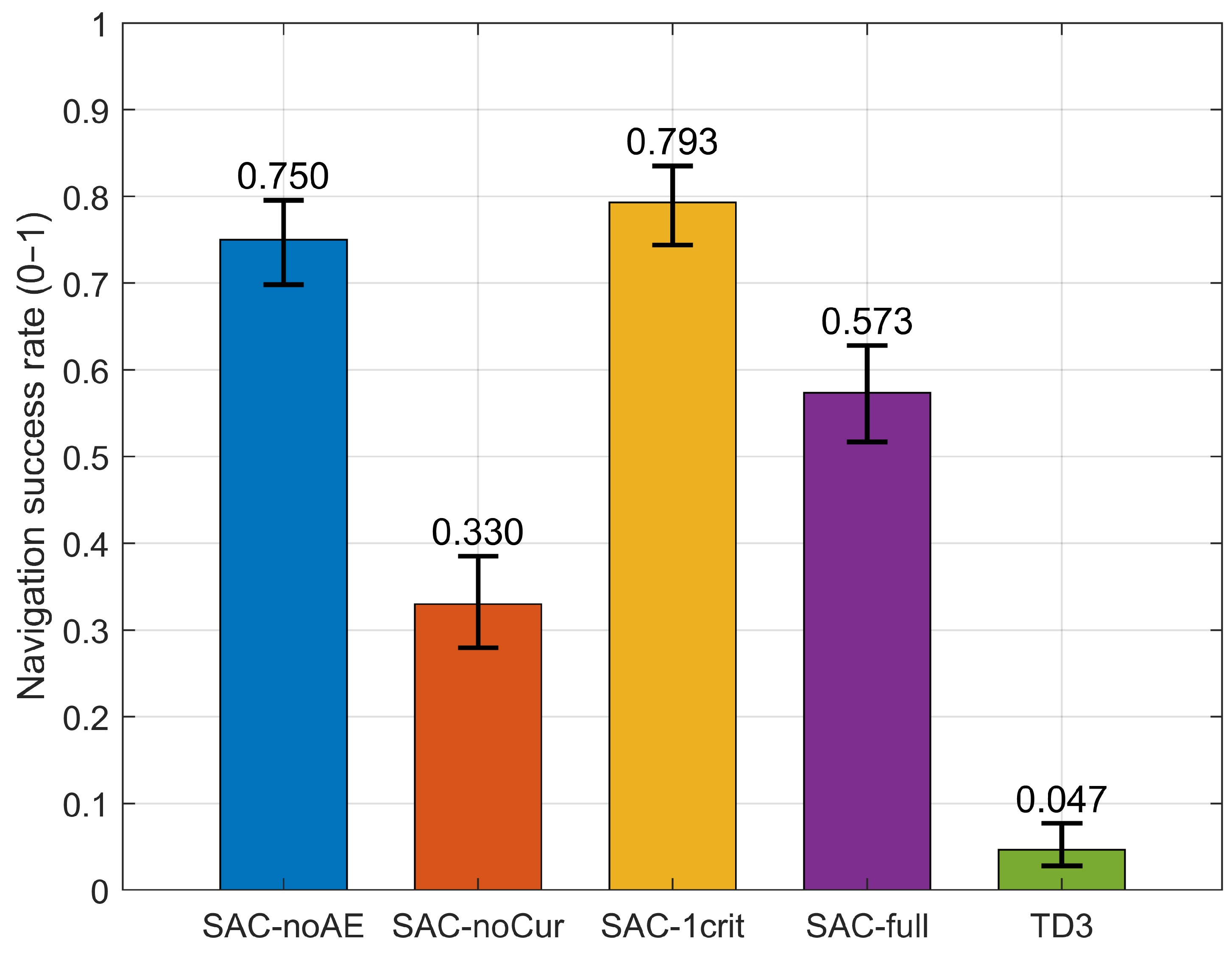
The navigation success rate $S_{\mathrm{nav}}$ exhibits statistically significant differences among the evaluated configurations (Figure 4). Among the SAC-based agents, SAC-1crit (SAC with a single critic) achieves the highest mean performance ($S_{\mathrm{nav}}=0.793$), followed by SAC-noAE (SAC without automatic entropy tuning) ($0.750$) and SAC-full (SAC with automatic entropy tuning, twin critics, and curriculum learning) ($0.573$). This pattern suggests that, for navigation, a single critic may favor more direct convergence by reducing the conservativeness induced by the combination of twin critics, entropy regularization, and curriculum learning.

However, this higher performance on the SAC-1crit task is achieved at the expense of reduced regularization. In contrast, SAC-full explicitly incorporates twin critics, automatic entropy tuning, and curriculum learning—mechanisms associated with global robustness and stability—which also facilitate coherent integration with the manipulation stage.

The relevance of curriculum learning is evidenced by the markedly lower performance of SAC-noCur (SAC without curriculum learning), which achieves only $S_{\mathrm{nav}}=0.330$. Compared with SAC-full, this result indicates that the lack of a controlled progression of difficulty leads to suboptimal policies, particularly during early phases sensitive to the environment’s spatial complexity.

TD3, in turn, exhibits a substantially lower success rate ($S_{\mathrm{nav}}=0.047$), confirming that a deterministic policy without entropy regularization or curriculum lacks the robustness required to operate reliably in unstructured and variable mining environments.

From a statistical standpoint, SAC-1crit shows a relatively narrow $95\%$ confidence interval $[0.744,0.835]$, indicating low inter-episode variability. SAC-noAE presents a compact $95\%$ CI $[0.698,0.796]$, suggesting that disabling automatic entropy does not compromise stability when the rest of the architecture is preserved. In contrast, SAC-noCur and TD3 exhibit greater dispersion, reflecting sensitivity to obstacle spatial distributions and environmental randomness.

In relative terms, the performance gap between the SAC-based agents and TD3 exceeds one order of magnitude, while the gap between SAC-1crit and SAC-full highlights a trade-off between convergence speed and structural robustness. Overall, the results confirm that curriculum learning and entropy regularization are decisive for stability, generalization, and operational reliability.

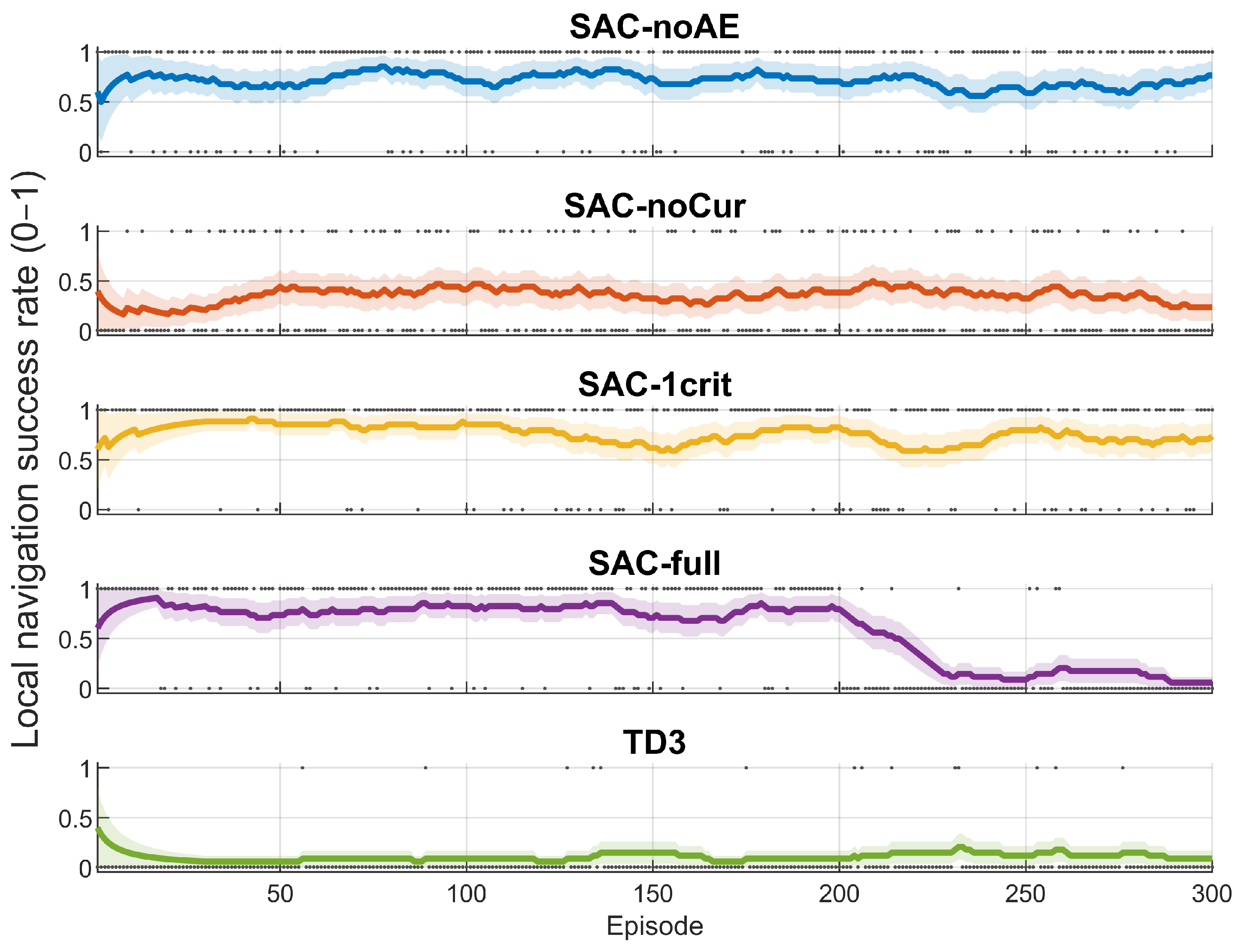
The temporal evolution of local success, estimated using a sliding window of 30 episodes with $95\%$ confidence intervals (Figure 5), further reinforces these conclusions. SAC-1crit maintains local success values predominantly within the range $S_{\mathrm{nav}}\in [0.7,0.85]$ for most episodes, with narrow uncertainty bands. Similarly, SAC-noAE exhibits sustained values in the approximate range $S_{\mathrm{nav}}\in [0.65,0.80]$.

The SAC-full agent, during early and intermediate episodes (approximately up to episode 150), shows a success rate comparable to SAC-noAE, typically around $S_{\mathrm{nav}}\in [0.65,0.75]$. However, in later stages, a progressive decrease in local success is observed, reaching values below $S_{\mathrm{nav}}\approx 0.30$ toward the final episodes. This sustained decline is consistent with the adoption of more conservative policies, induced by the combined effect of twin critics, automatic entropy regularization, and curriculum learning.

In contrast, the SAC-noCur agent presents significantly lower and more variable temporal performance, with success rates rarely exceeding $S_{\mathrm{nav}}\approx 0.45$ and wide uncertainty bands. This behavior reflects the agent’s difficulty in adapting to increasingly complex environments without a curriculum.

The TD3 agent remains persistently low, typically below $S_{\mathrm{nav}}\approx 0.10$, with irregular oscillations and no clear stabilization trend across episodes. This pattern confirms that deterministic policies without entropy regularization or curriculum learning lack the robustness needed to sustain reliable performance in unstructured, highly variable mining scenarios.

Overall, this temporal analysis confirms that the differences observed in the aggregated metrics do not reflect isolated or transient effects, but rather reflect the structural properties of stability, robustness, and consistency inherent to each evaluated navigation agent architecture.

4.4.2. Distance Reduction Toward the Target

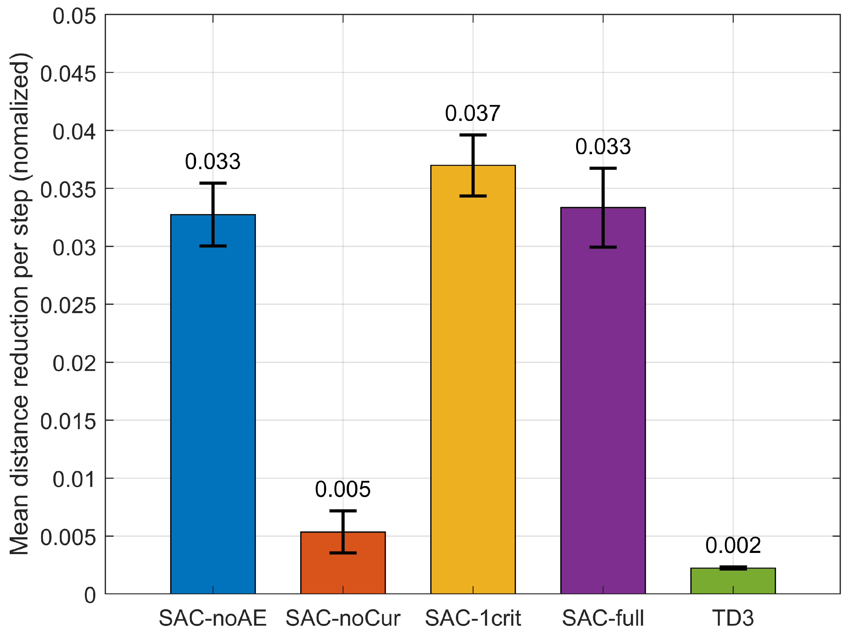
The mean distance reduction rate per step $R_d$ evaluates the kinematic efficiency with which each agent guides the machinery toward the target, independently of the final episode success (Figure 6).

SAC-noAE, SAC-1crit, and SAC-full exhibit values of the same order of magnitude ($0.0327$–$0.0370$). SAC-1crit achieves the highest mean value, $R_d=0.0370$ with $95\%$ CI $\approx [0.0345,0.0398]$, consistent with a more direct approach and high navigation success.

SAC-full attains an intermediate value, $R_d=0.0333$ with $95\%$ CI $\approx [0.0300,0.0368]$, suggesting more conservative trajectories due to regularization and curriculum learning. In contrast, SAC-noCur presents a substantially lower distance reduction ($R_d=0.0053$), evidencing poorly structured trajectories and erratic progress, consistent with the absence of curriculum learning.

TD3 shows the worst performance ($R_d=0.0022$), confirming that a deterministic policy without entropy regularization or progressive structuring fails to achieve consistent goal-oriented motion in unstructured environments.

Overall, these results indicate that while several SAC-based agents can sustainably reduce the distance to the target, architectural differences directly influence approach efficiency, complementing the global success results and reinforcing the roles of curriculum learning and critic design in generating effective trajectories.

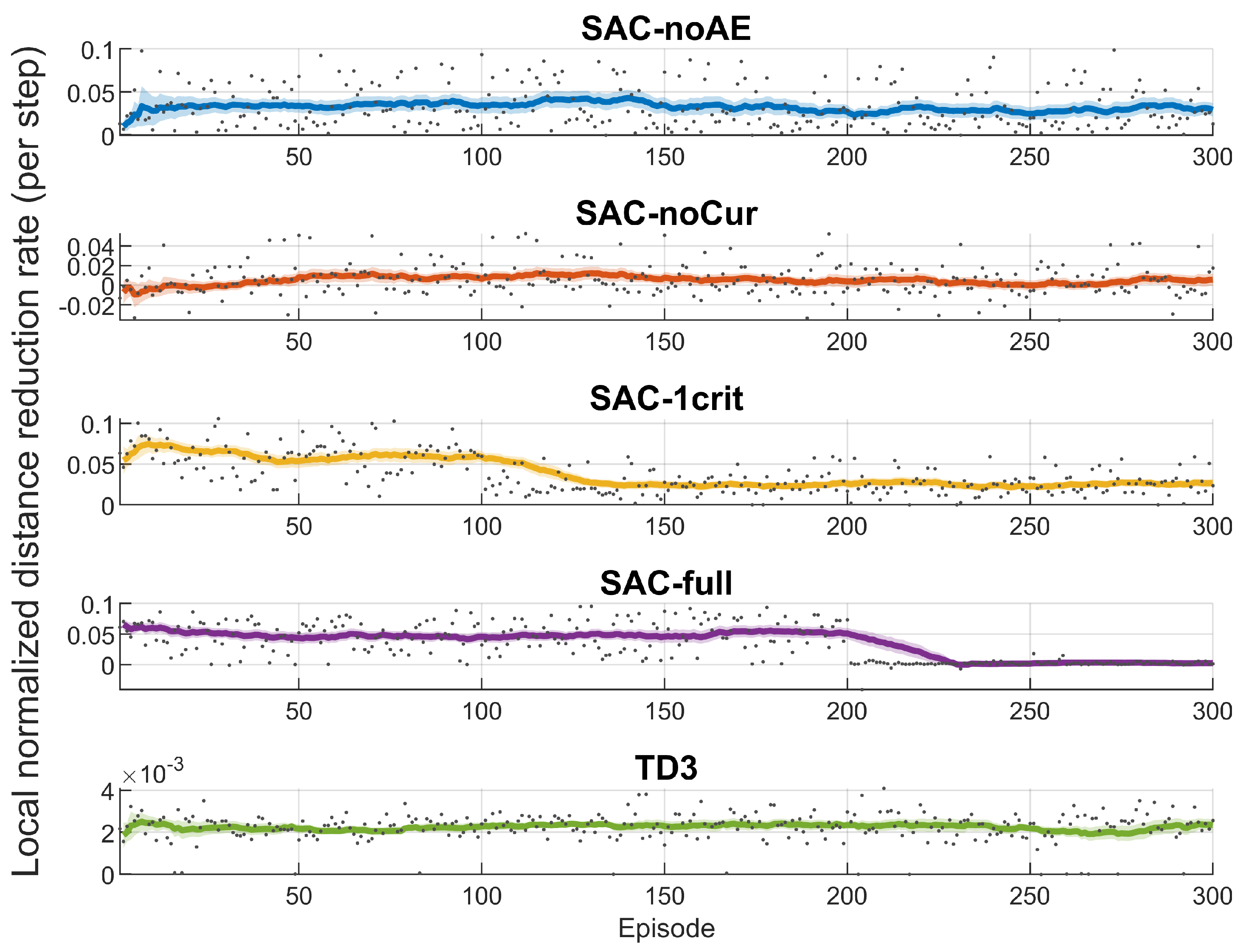
The temporal evolution of $R_d$ using a 30-episode sliding window with $95\%$ confidence intervals (Figure 7) complements the averaged results. SAC-noAE and SAC-1crit maintain stable, positive values over time. In particular, SAC-1crit exhibits local values predominantly oscillating within the range $R_d\approx 0.03$–$0.06$ during the first 100–120 episodes, followed by stabilization around $R_d\approx [0.025,0.035]$, while maintaining narrow uncertainty bands. Similarly, SAC-noAE shows a stable temporal trajectory, with values between $R_d\approx 0.03$–$0.045$, and no significant degradation toward the final episodes. The stability of both configurations confirms that disabling automatic entropy tuning or using a single critic does not compromise the agent’s ability to generate progressive and goal-oriented trajectories during navigation.

SAC-full displays a clearly differentiated pattern: In the early stages, it maintains $R_d$ values comparable to SAC-1crit ($R_d\approx 0.04$–$0.06$), followed by a progressive reduction toward values close to zero in the final episodes. This behavior is consistent with a more conservative policy, in which the combination of twin critics, automatic entropy tuning, and curriculum learning favors cautious navigation strategies that prioritize stability and collision avoidance over approach speed.

The SAC-noCur agent exhibits a distinct dynamic, with values oscillating around zero throughout the entire horizon, typically within the range $-0.01\le R_d\le 0.02$, and with considerably higher dispersion. This lack of sustained directionality confirms that the absence of curriculum learning prevents the acquisition of consistent approach strategies.

The TD3 agent maintains nearly constant values near zero ($R_d\approx 0.001$–$0.003$) across all episodes, with no evidence of progressive improvement or meaningful stabilization. This result reinforces the conclusion that a deterministic policy without regularization is inadequate for generating efficient trajectories in highly variable, unstructured mining scenarios.

Overall, the temporal analysis confirms that the ability to consistently reduce the distance to the target is not a transient or isolated effect, but rather a structural property of architectures that incorporate curriculum learning and an appropriate critic design. The metric $R_d$ thus emerges as a sensitive indicator of the quality, efficiency, and stability of the trajectories learned by the different navigation agents.

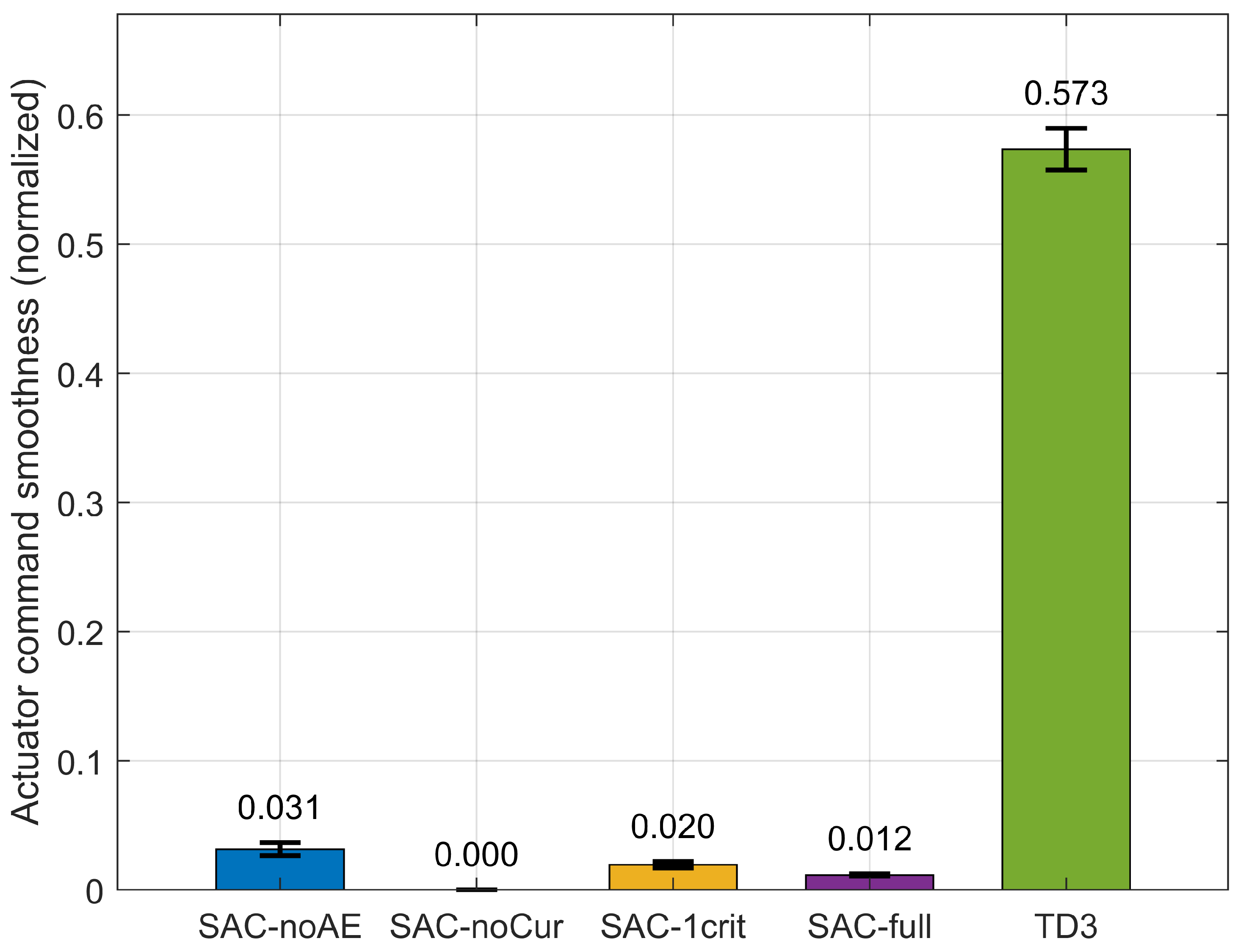
4.4.3. Actuator Smoothness in Navigation

The smoothness of the commands during navigation was evaluated using the indicator ${\xi }_{\tau }$, which quantifies the temporal variation between consecutive actions and, consequently, the level of dynamic effort applied to the actuators (Figure 8).

All SAC variants exhibit low values of ${\xi }_{\tau }$ (between $0.012$ and $0.031$). In particular, SAC-full achieves the lowest mean value (${\xi }_{\tau }=0.012$), followed by SAC-1crit ($0.020$) and SAC-noAE ($0.031$), all with narrow confidence intervals, indicating stable and reproducible behavior.

These results suggest that SAC induces smooth, progressive control policies that avoid abrupt command changes. In contrast, TD3 reaches ${\xi }_{\tau }\approx 0.573$, approximately 18–45 times larger, reflecting large-amplitude oscillations and a more reactive, less damped deterministic policy under uncertainty.

Overall, this analysis confirms that the maximum-entropy formulation not only promotes exploration but also leads to smoother, more stable control actions, which are particularly relevant for safe operation and actuator longevity.

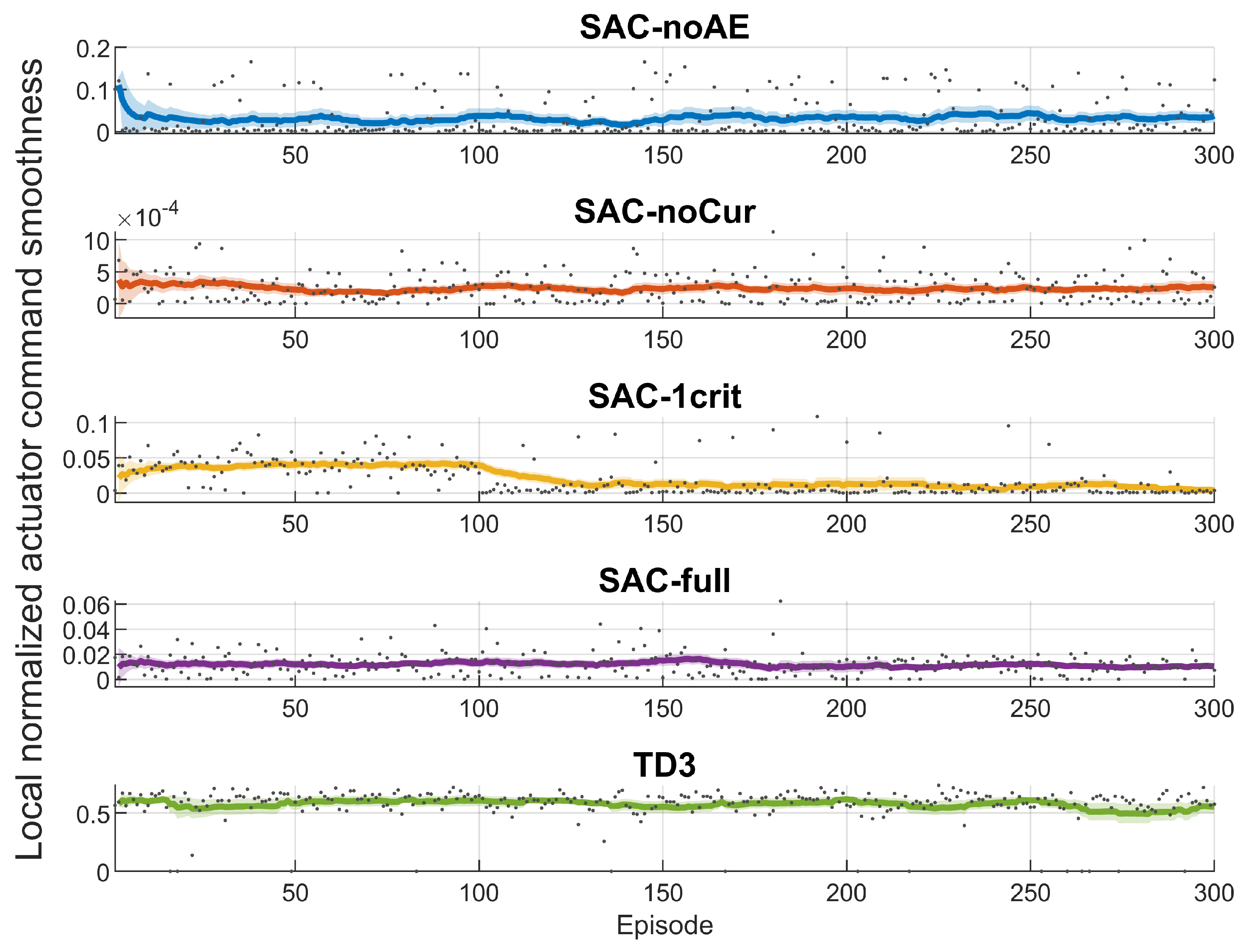
The temporal evolution of ${\xi }_{\tau }$, estimated using a sliding window of 30 episodes with 95% confidence intervals (Figure 9), further reinforces these observations. All SAC variants exhibit a quasi-stationary behavior. In particular, SAC-full maintains values below ${\xi }_{\tau }\approx 0.02$ with narrow uncertainty bands, indicating a stable and well-regularized control policy. Similarly, SAC-1crit converges rapidly to values within ${\xi }_{\tau }\in [0.01,0.03]$, showing a slight decrease during the first 100 episodes before stabilizing.

SAC-noAE presents values in the range ${\xi }_{\tau }\approx 0.03$–$0.05$, especially during the initial episodes, with bounded and relatively narrow confidence intervals. This suggests that the absence of automatic entropy tuning does not induce instabilities or significant oscillations in the control actions.

In contrast, SAC-noCur exhibits greater dispersion and temporal variability (on the order of ${10}^{-4}$). This behavior indicates that, although the action magnitudes remain smooth, the lack of curriculum learning leads to a less consistent temporal structure in the control policy, likely due to early exposure to complex scenarios before robust navigation primitives are fully established.

The TD3 agent shows a markedly different temporal profile, with persistently high values (${\xi }_{\tau }\approx 0.5$–$0.6$), wide confidence intervals, and no clear convergence trend. These sustained oscillations reflect frequent abrupt changes in control signals, characteristic of a reactive deterministic policy operating under uncertainty.

Overall, the temporal analysis confirms that SAC produces smooth, temporally stable control policies, whereas deterministic methods such as TD3 exhibit high, persistent variability in actuation signals.

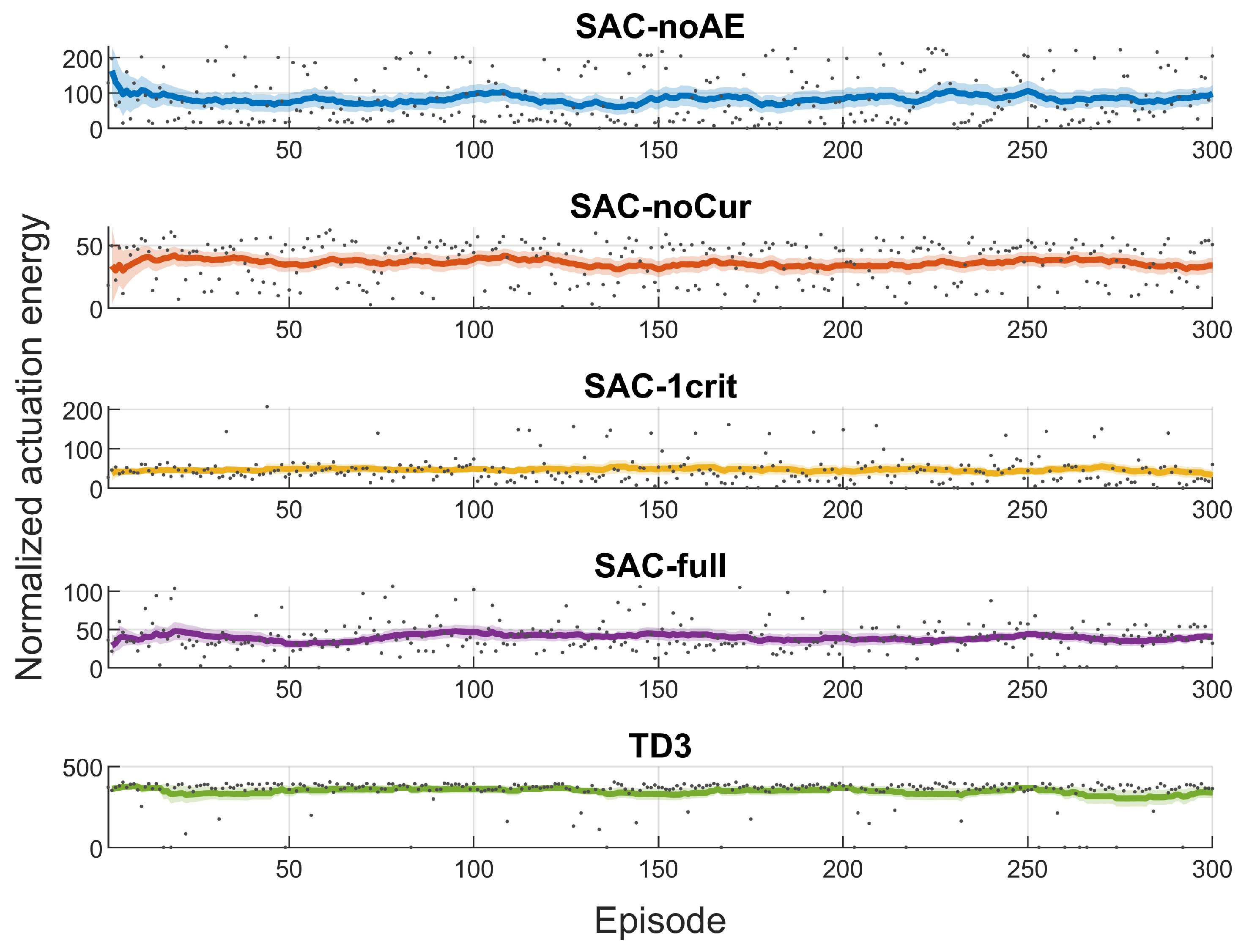
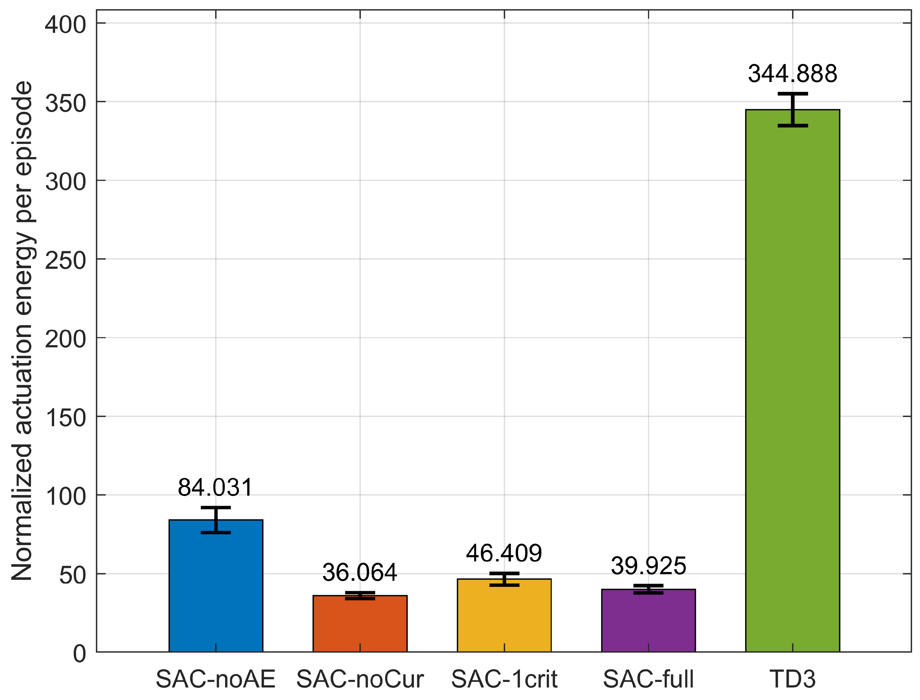
4.4.4. Navigation Actuation Energy

The actuation energy $E_{\tau }$ measures the mechanical effort required by each policy during navigation (Figure 10) and is particularly relevant in mining machinery due to energy consumption and mechanical wear. The SAC architectures exhibit moderate and bounded energy consumption (36.1–84.0 units per episode). In particular, SAC-noCur and SAC-full achieve the lowest mean energy levels ($E_{\tau }=36.1$ and $E_{\tau }=39.9$, respectively), reflecting policies that favor smooth and progressive trajectories while avoiding unnecessary accelerations during the displacement toward the target.

SAC-1crit shows a higher energy consumption ($E_{\tau }=46.4$), consistent with the more direct and decisive strategy observed in the distance-reduction indicators. In contrast, SAC-noAE reaches the highest energy consumption among the SAC variants ($E_{\tau }=84.0$), suggesting a more aggressive policy, especially during the initial phases of the episode, where exploration not regulated by entropy induces higher-amplitude commands.

The TD3 agent records an extremely high actuation energy ($E_{\tau }=344.9$), nearly an order of magnitude larger than SAC. This difference confirms that the deterministic policy generates persistent oscillations and large-amplitude actions, leading to excessive mechanical effort and inefficient actuator use.

Overall, these results demonstrate that the SAC framework, through entropy regularization and explicit penalization of control effort, not only improves robustness and stability in navigation but also significantly reduces energy consumption—an essential aspect for the practical viability of autonomous systems in real mining environments.

The temporal evolution of the actuation energy $E_{\tau }$, estimated using a sliding window of 30 episodes with 95% confidence intervals (Figure 11), reinforces the bounded energy profiles observed for the SAC-based agents. In particular, SAC-noCur, SAC-1crit, and SAC-full exhibit values that fluctuate within relatively narrow ranges and exhibit reduced confidence bands, indicating consistent behavior across different obstacle configurations and randomized initial conditions. The SAC-noAE agent shows slightly higher energy levels, with fluctuations around 80–120 units, but without exhibiting divergent trends or progressive instabilities.

In contrast, TD3 displays persistently high energy levels, exceeding 300 units and reaching peaks of 400–450 units. Moreover, its temporal profile exhibits substantial variability and lacks a clear decreasing trend, suggesting that the TD3 policy fails to internalize effective mechanisms for self-regulation of actuation effort.

4.5. SAC-2 Results (Manipulation)

4.5.1. Manipulation Success Rate

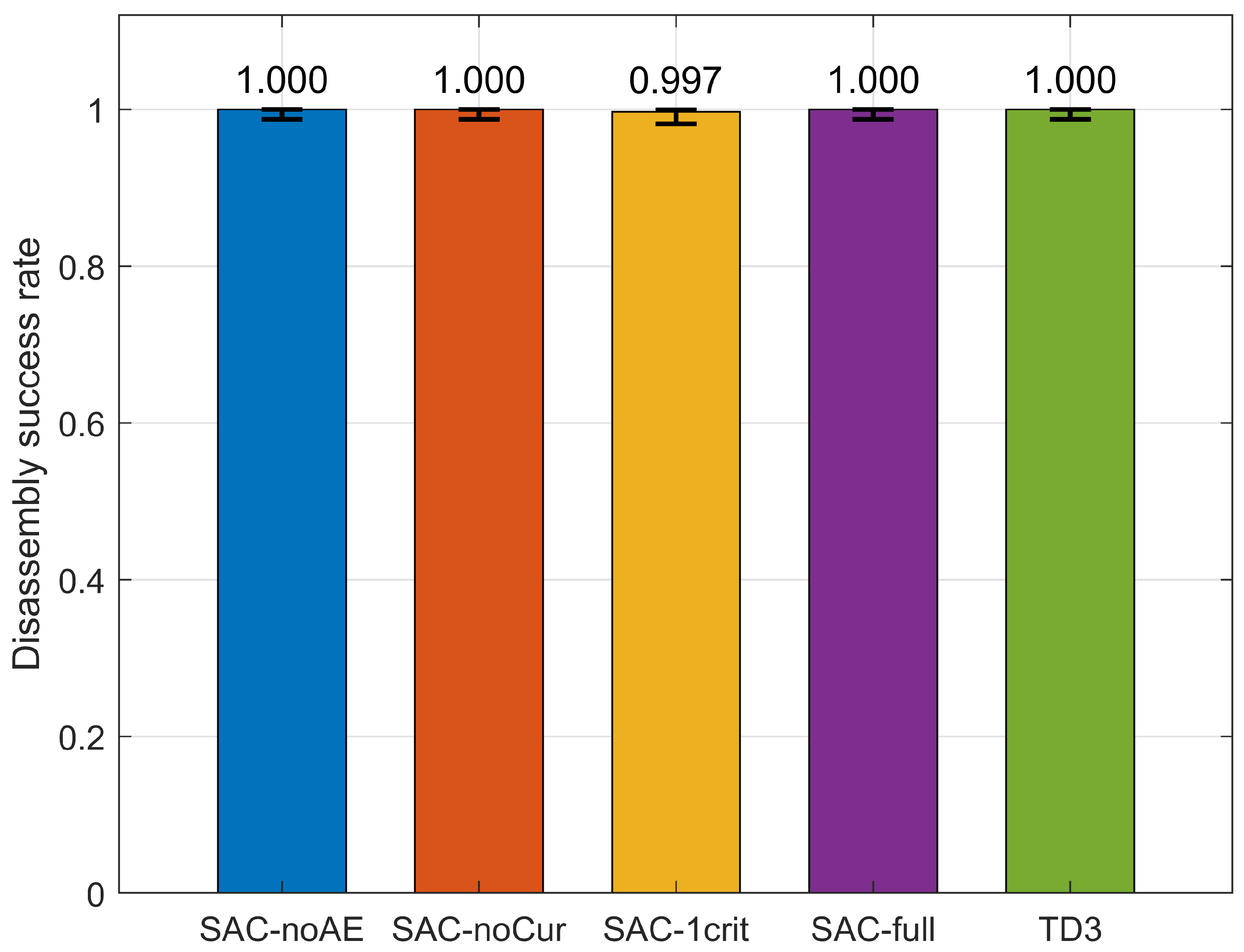
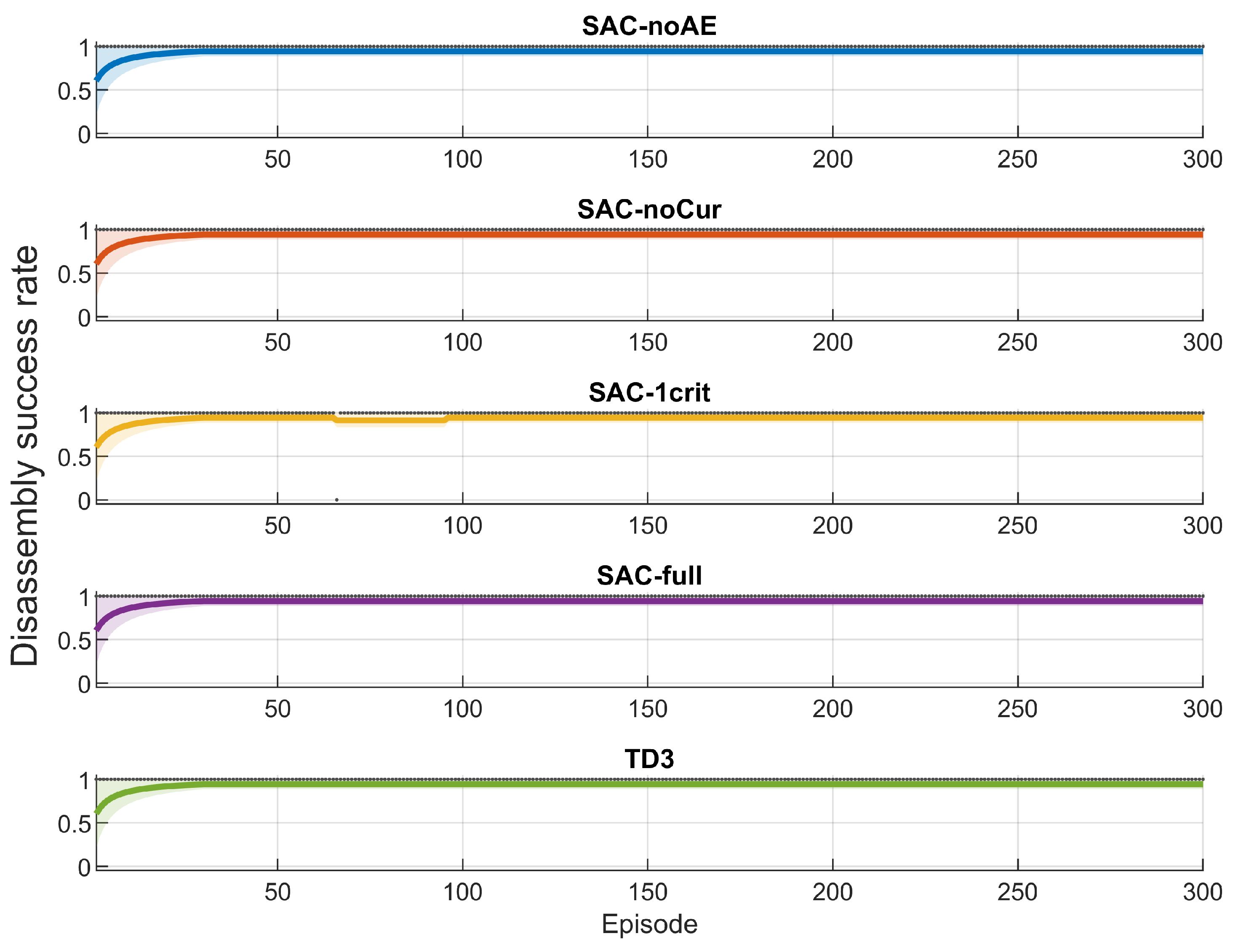
The disassembly success rate $S_{\mathrm{dis}}$ indicates that all evaluated configurations consistently complete the rock pile fragmentation task (Figure 12). Both the SAC-based variants and TD3 achieve mean values between $0.997$ and $1.000$, indicating near-perfect completion of the objective defined by the height threshold $h_{\mathrm{thr}}$. The Wilson 95% confidence intervals remain above $0.98$, evidencing low variability and high robustness across different initial conditions. In particular, SAC-noAE, SAC-noCur, SAC-full, and TD3 achieve a success rate of $1.000$, while SAC-1crit exhibits a marginally lower rate ($0.997$); this difference is not statistically significant given the overlap of the confidence intervals.

This behavior indicates that the metric $S_{\mathrm{dis}}$ suffers from a saturation effect and does not adequately discriminate among agents in terms of the quality of the learned policy.

The temporal evolution of $S_{\mathrm{dis}}$, estimated using a sliding window of 30 episodes with 95% confidence intervals (Figure 13), further confirms this saturation effect: all curves rapidly converge to values close to 1 and remain there with only marginal oscillations and narrow uncertainty bands. From a quantitative standpoint, the largest difference observed among models corresponds to approximately $0.3\%$ of episodes in which complete disassembly is not achieved.

This behavior confirms that, under the considered simulation conditions, the disassembly task is not limiting in terms of reachability. Consequently, additional dynamic metrics—such as the height reduction rate, torque smoothness, and actuation energy—are more informative for discriminating among policies and for assessing the quality of the control learned by each agent.

4.5.2. Height Reduction

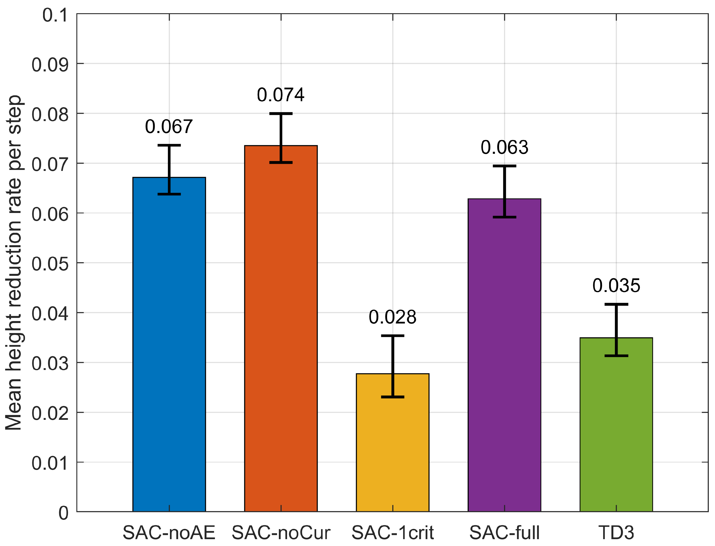
The height reduction rate $R_h$ constitutes a substantially more informative metric than the binary disassembly rate, as it quantifies the dynamic efficiency of the disassembly process (Figure 14).

The SAC variants exhibit the highest values of $R_h$ ($0.0628$–$0.0735$) units of height reduced per simulation step. SAC-noCur achieves the highest value ($0.0735$), followed by SAC-noAE ($0.0672$) and SAC-full ($0.0628$), indicating that, once in steady state, these agents can exert effective impact in a sustained manner.

SAC-1crit presents the lowest value ($0.0277$), suggesting a less efficient strategy despite completing the disassembly task. TD3 achieves an intermediate value ($0.0349$), lower than the SAC configurations, reflecting a reduced ability to convert actuation effort into effective height reduction of the rock pile.

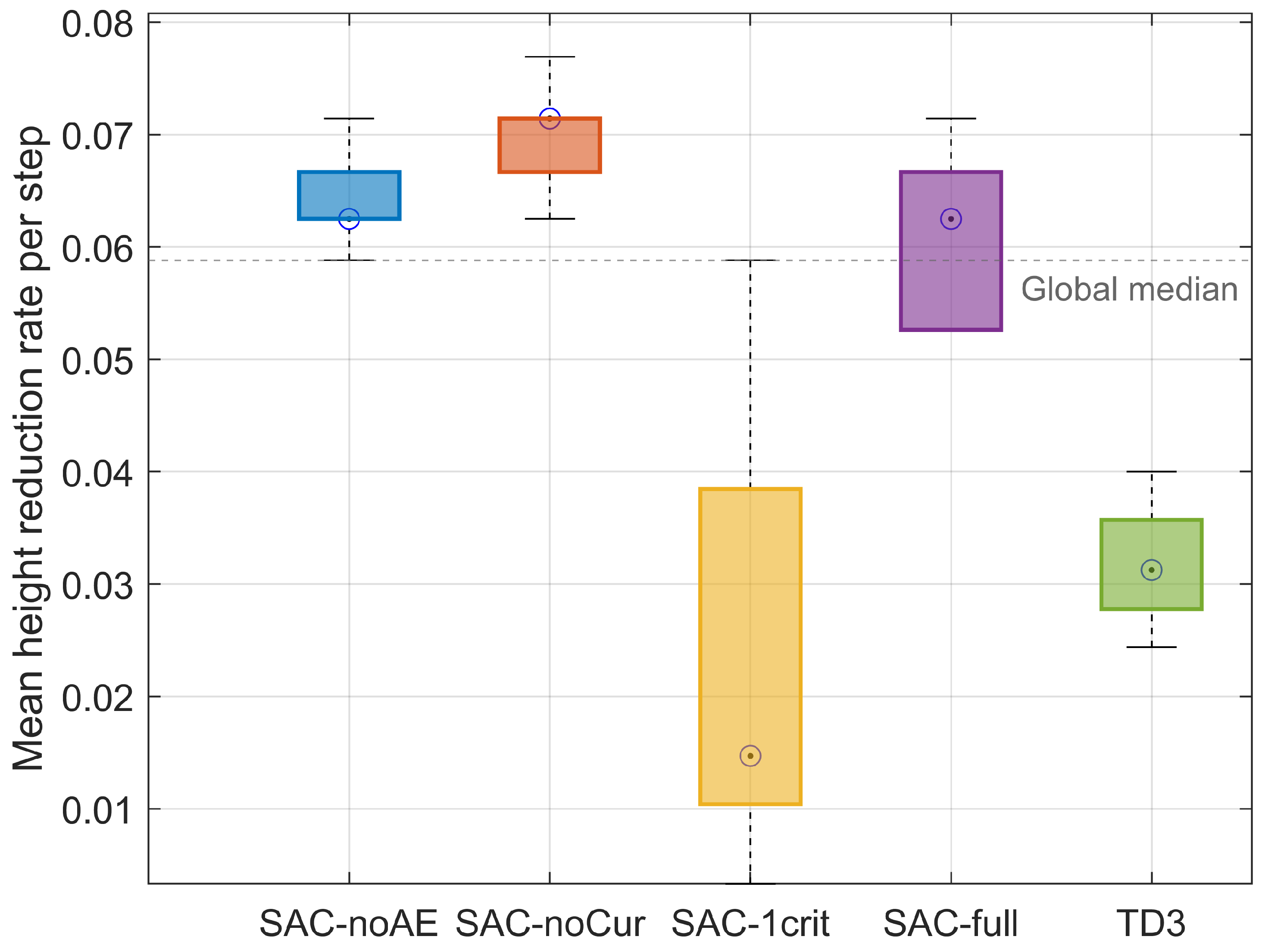
The inspection of the episode-level distribution of $R_h$ using box plots (Figure 15) reinforces and further qualifies the results obtained from the mean values. The SAC-noAE, SAC-noCur, and SAC-full agents exhibit high medians above the global median and compact interquartile ranges, indicating consistent height reduction across episodes and low intra-policy variability.

SAC-noCur stands out by concentrating its distribution in the upper region of $R_h$, confirming its high dynamic efficiency during the disassembly phase. Nevertheless, this behavior must be interpreted within the context of the complete system, since the absence of curriculum learning negatively affects the overall performance of the hierarchical scheme, as evidenced by the navigation results.

SAC-1crit exhibits significantly greater dispersion, with a lower median and a pronounced lower tail, indicating episodes with slow or ineffective height reduction. This suggests a less robust strategy with respect to variations in pile geometry. The TD3 agent, although exhibiting a more concentrated distribution than SAC-1crit, is shifted toward lower $R_h$ values, indicating a lower average efficiency in the disassembly process.

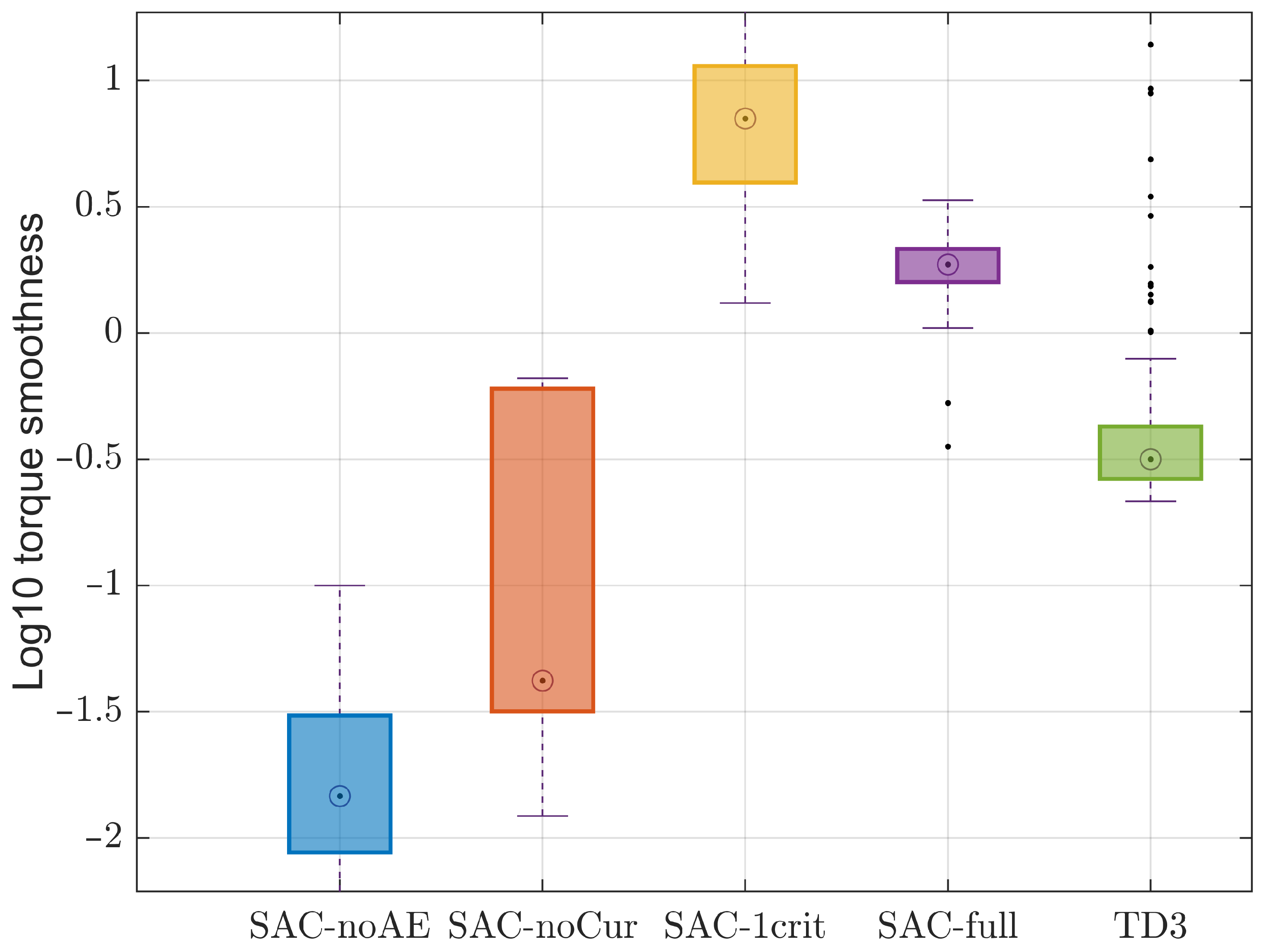
4.5.3. Actuator Smoothness

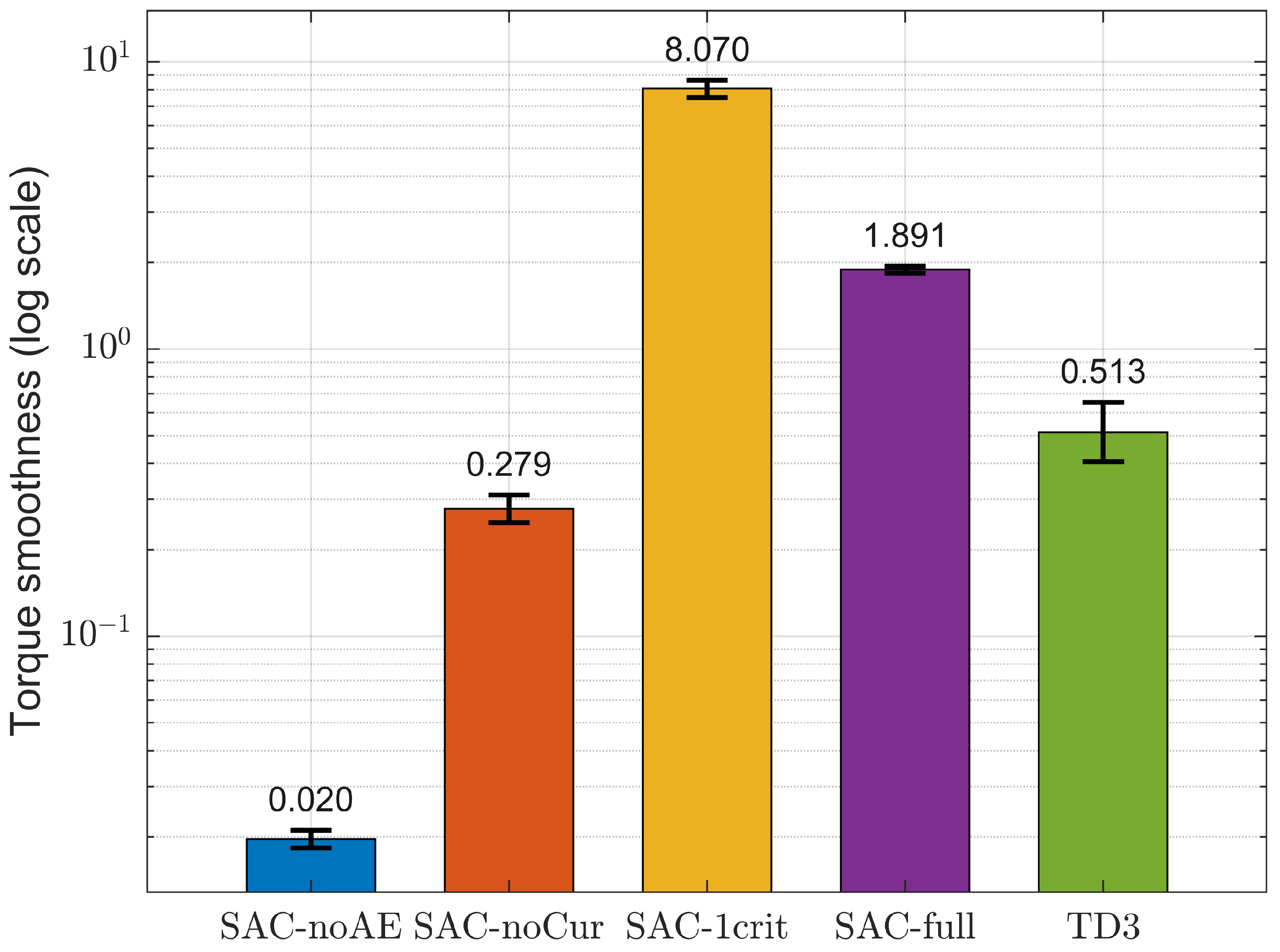
The smoothness of the hydraulic actuators was evaluated using the index ${\xi }_{\tau }$, defined by the variation between consecutive torque commands. Since the differences span several orders of magnitude, the aggregated results are presented on a logarithmic scale (Figure 16).

The SAC-noAE agent exhibits the lowest ${\xi }_{\tau }$ ($\approx 1.97\times {10}^{-2}$), indicating a highly damped policy with very smooth torque transitions. SAC-noCur and TD3 are located at an intermediate level ($\approx 2.79\times {10}^{-1}$ and $5.13\times {10}^{-1}$, respectively), reflecting more variable but still bounded command profiles. In contrast, SAC-1crit and SAC-full exhibit the highest values ($\approx 8.07$ and $1.89$, respectively), corresponding to a more aggressive control regime with higher temporal variation.

These results show that the algorithmic components affect not only the efficiency of the disassembly process but also the dynamic profile of the control actions. In particular, disabling automatic entropy tuning favors markedly smoother policies, whereas using a single critic or the full SAC configuration tends to generate more reactive commands. This trade-off aligns with trends in $R_h$ and underscores the need to jointly assess process performance and the mechanical demands imposed on the system.

The distributional analysis of ${log}_{10}\left({\xi }_{\tau }\right)$ (Figure 17) confirms the presence of significant differences among the evaluated agents. SAC-noAE concentrates most episodes in the region of lowest torque variability, with a narrow dispersion. This behavior evidences consistent, well-damped, and physically plausible actuation dynamics, particularly suitable for hydraulic systems operating under severe mechanical constraints.

SAC-1crit exhibits a markedly larger dispersion with extended tails toward higher values, indicative of more abrupt transients and a more aggressive control regime. Such behavior implies a higher potential for mechanical stress on the actuation system.

The SAC-noCur and SAC-full configurations occupy intermediate positions: both retain the majority of episodes within moderate ranges of ${\xi }_{\tau }$, albeit with greater dispersion than SAC-noAE. TD3, in contrast, displays a distribution shifted toward higher values and includes extreme episodes, reflecting a less damped control policy with higher temporal variability in torque commands.

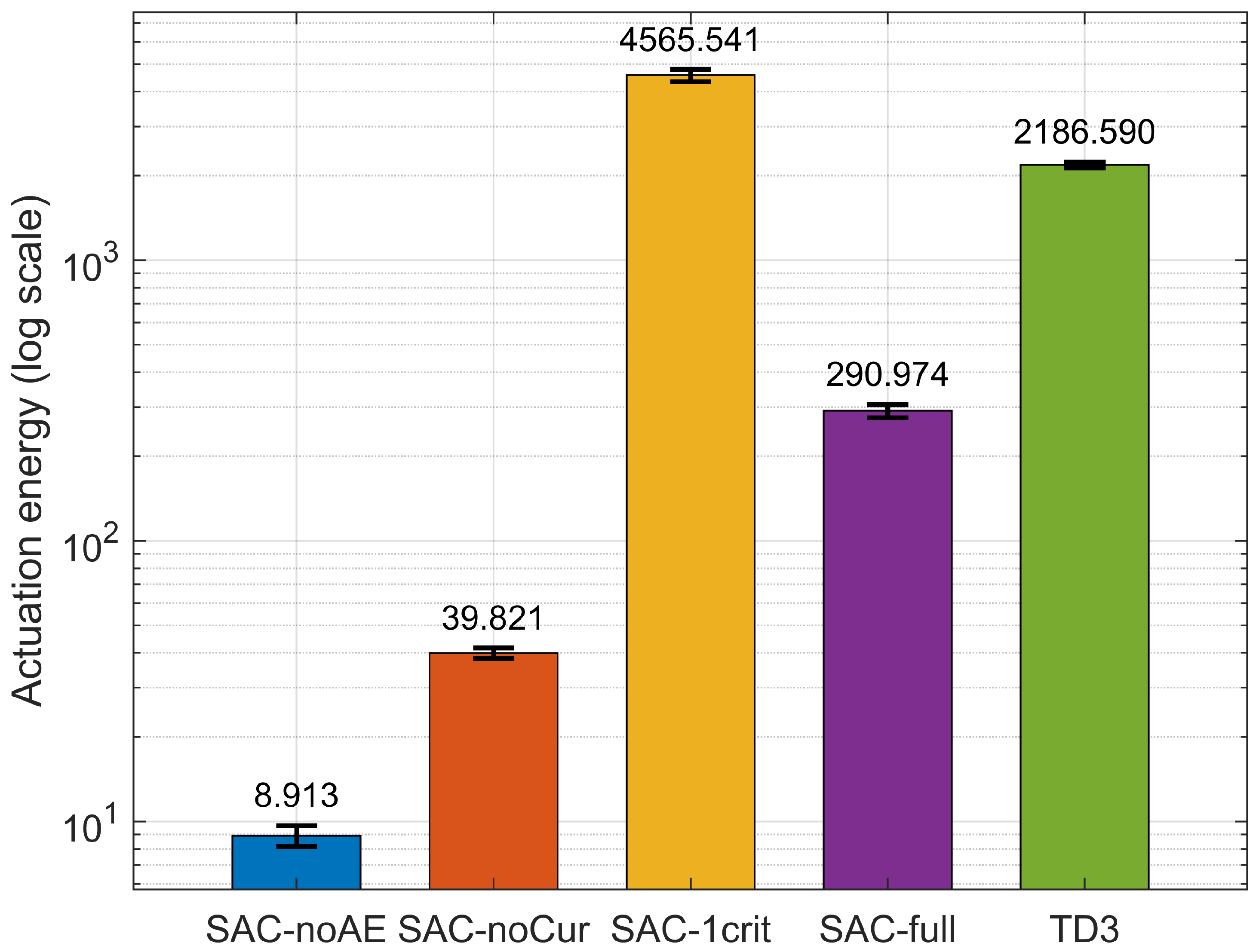
4.5.4. Manipulation Actuation Energy

The actuation energy $E_{\tau }$ measures the energetic/mechanical demand of each policy during the disassembly phase and is reported on a logarithmic scale (Figure 18).

SAC-noAE exhibits the lowest mean consumption ($E_{\tau }\approx 8.9$), followed by SAC-noCur ($\approx 39.8$), indicating efficient policies with moderate torque usage. In contrast, SAC-full reaches a substantially higher consumption level ($\approx 291$), while SAC-1crit attains the largest overall value ($\approx 4565$), consistent with a particularly demanding, aggressive actuation regime. TD3 also shows high energy consumption ($\approx 2186$), confirming its limited ability to regulate actuation effort.

Taken together, these results indicate that, although all configurations achieve near-perfect success rates in the disassembly task, there exist differences of several orders of magnitude in energy cost. This finding underscores the importance of considering continuous metrics such as $E_{\tau }$ when assessing the operational feasibility of autonomous systems in real-world applications.

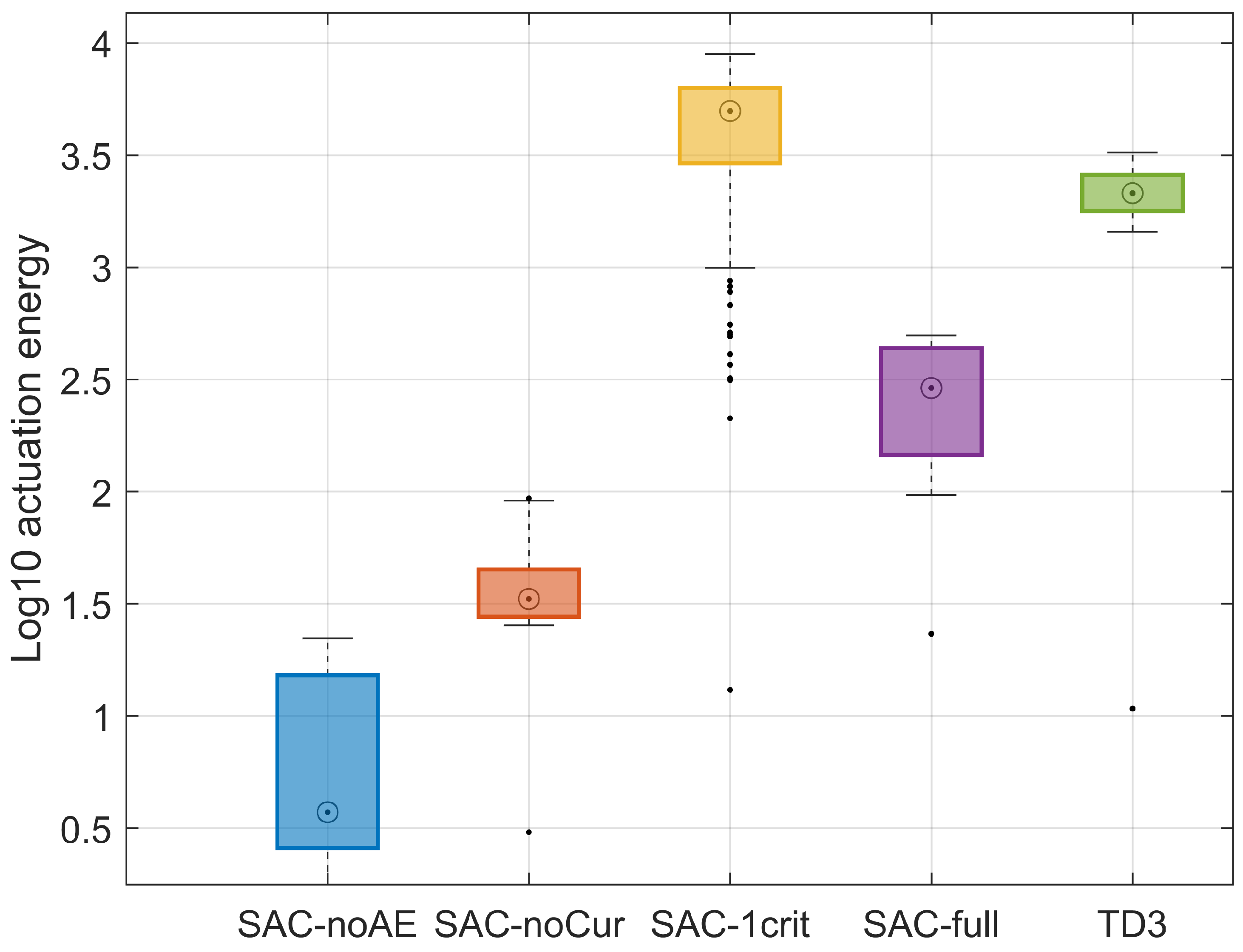
The distributional analysis of $E_{\tau }$ on a logarithmic scale (Figure 19) confirms that these differences also affect inter-episode variability. SAC-1crit exhibits the largest dispersion and a pronounced presence of outliers toward high energy levels, reflecting episodes with actuation demands far above the average. In contrast, SAC-noAE shows a compact distribution concentrated in the low-energy region, evidencing consistency and energetic efficiency. The SAC-noCur and SAC-full configurations present intermediate dispersion, while TD3 maintains a distribution shifted toward higher energy requirements.

Overall, $E_{\tau }$ emerges as a sensitive indicator of the actuation regime and of the impact of algorithmic components on energy efficiency and the stability of the disassembly process.

5. Discussion

5.1. Navigation Agents

The ablation study enables isolating the effect of each architectural component on the performance of the SAC-1 subagent. SAC-full offers the most balanced profile, combining competitive performance with temporal stability, control smoothness, and bounded energy consumption—properties that are particularly relevant for industrial mobile machinery, where reliability and operational safety are often more valuable than marginal improvements in a single metric.

Removing curriculum learning (SAC-noCur) results in the greatest degradation in navigation performance, reducing the success rate to less than half and significantly impairing directional efficiency. This confirms that the curriculum not only accelerates learning but also imposes a progressive structure of difficulty that prevents poorly formed early policies and stabilizes the acquisition of goal-oriented behaviors.

Suppressing automatic entropy tuning (SAC-noAE) preserves competitive success rates but increases energy consumption, consistent with a more aggressive control regime. This suggests that entropy plays a dual role: it promotes exploration during training and acts as a regulator of control intensity, preventing unnecessary increases in mechanical effort.

The single-critic variant (SAC-1crit) maximizes $R_d$, evidencing more direct trajectories, but exhibits higher sensitivity to initial conditions and obstacle layouts. This outcome is consistent with the motivation for using double critics to mitigate overestimation and reduce variability in highly stochastic environments. From an operational standpoint, this variant may be attractive when a rapid approach is the primary objective, albeit at the cost of reduced robustness.

TD3 serves as a contrasting reference: its deterministic policy, lacking entropy regularization and curriculum learning, exhibits the worst overall performance, with unstable trajectories and high mechanical costs. In this unstructured environment, the results support the conclusion that the combination of regularized exploration and progressive learning is critical for stability and reliability.

In summary, for autonomous navigation, each component fulfills a functional role: the curriculum supports generalization, entropy regulates actuation intensity, and double critics enhance robustness under uncertainty. Under operational criteria, SAC-full emerges as the most balanced option.

5.2. Disassembly Agents

In the disassembly subagent (SAC-2), all variants achieve success rates $S_{\mathrm{dis}}>99\%$, indicating that, under the simulated conditions considered, the binary success metric is saturated and does not adequately discriminate between policies. Consequently, the analysis must focus on continuous metrics such as height reduction ($R_h$), torque smoothness (${\xi }_{\tau }$), and actuation energy ($E_{\tau }$), which better capture process efficiency and the dynamic quality of hydraulic control.

Removing curriculum learning (SAC-noCur) does not prevent task completion. However, it reduces disassembly’s dynamic efficiency and increases the dependence of performance on the episode configuration, consistent with the loss of progressive structure during learning. In contrast, SAC-noAE stands out for exhibiting the smoothest and most energy-efficient regime, which is desirable from a mechanical standpoint; however, the achieved height reduction tends to be less pronounced, suggesting a more conservative control strategy.

The SAC-1crit variant exhibits the most aggressive behavior: it achieves height reduction but with higher torque variability and the highest energy cost. From a transfer perspective, this could translate into accelerated wear and increased hydraulic demands, making it less suitable when operational objectives include system preservation. TD3, despite completing the disassembly task, shows lower efficiency and greater actuation irregularity, reinforcing the advantage of regularized stochastic policies in maintaining a more controlled dynamic regime.

In summary, for SAC-2, the final success rate is not the limiting factor; rather, the discriminative criterion is the process’s dynamic quality. Under this framework, SAC-full again emerges as the most suitable alternative, balancing efficiency, stability, and energy cost—criteria well aligned with potential transfer to real-world comminution scenarios.

6. Limitations

6.1. Navigation Agent

The autonomous navigation module based on deep reinforcement learning exhibits several limitations stemming from the modeling, perception, and training choices adopted in this study. First, the environment relies on a simplified kinematic model of a tracked vehicle, where actions are interpreted as normalized accelerations directly integrated into each track’s velocity. This approach does not account for relevant dynamic effects, such as vehicle mass and inertia, track–ground contact forces, or the influence of slopes and terrain irregularities. As a result, the learned policy is valid under idealized kinematic assumptions, and its direct transfer to real platforms would require additional adaptation.

Regarding perception, the agent is provided with a structured and idealized state representation that includes obstacle positions, normalized heights, and the relative geometry of the target. Sensor noise, occlusions, and latency effects are not considered. While this choice simplifies learning and enables a controlled analysis, it may lead to an overestimation of performance under real sensing conditions. It should be noted that, even with idealized observations, the problem is still formulated as a POMDP, since in realistic scenarios there may exist unmodeled dynamics, terrain conditions, and disturbances that are not part of the observed vector. Therefore, the learned policy must be interpreted as being conditioned on a partial observation of the underlying physical state.

Additionally, the representation of the navigation environment is limited in terms of complexity and variability. The maximum number of obstacles is bounded; obstacles are static, and their geometry remains constant throughout each episode. Interactions between obstacles, contact-induced displacements, and topological changes in the environment are not modeled. Although a curriculum learning scheme is incorporated, it is implemented deterministically as a function of the episode count rather than the agent’s performance, potentially leading to mismatches between the environment’s difficulty level and the policy’s actual learning capability during training.

Furthermore, the reward function includes multiple carefully tuned reward-shaping terms, including progress toward the goal, angular alignment, action-smoothness penalties, temporal penalties, and terminal rewards for success. While this design promotes stability and convergence, it introduces a dependence on manually selected weights. It may bias the policy toward the specific task definition, potentially reducing generalization when operational criteria change.

Finally, training is computationally demanding due to the use of deep neural networks, large experience replay buffers, and extensive minibatches. This limits reproducibility on lower-capacity hardware and constrains systematic exploration of hyperparameter sensitivity.

6.2. Disassembly Agent

The disassembly module presents several limitations arising from the simplification of the dynamic model, the abstraction of contact interactions, and the specific representation of rock material. The manipulator dynamics are modeled using decoupled second-order equations for the yaw and pitch axes, including inertia, viscous damping, and gravity terms. This model neglects dynamic coupling between joints, centrifugal and Coriolis effects, inertia variations, and nonlinearities inherent to hydraulic actuators. As a result, the learned policy reflects an idealized dynamic behavior that may differ from that of a real physical system.

The interaction between the tool and the rock pile is represented by a discrete impact model based on geometric rules and thresholds (impact depth and centering) that determine the partial or total removal of material layers. This approximation does not model continuous contact forces, friction, deformations, progressive fragmentation, or lateral collapses, effectively reducing the disassembly process to deterministic simulator-dependent events. Consequently, there is a risk of overfitting the policy to these specific impact conditions, limiting its direct applicability to more realistic scenarios with granular physics.

Furthermore, the material pile is abstracted as a vertical layered structure with fixed geometry and a constant center, without representing the spatial distribution of fragments or changes in the center of mass during disassembly. The workspace, along with joint ranges and target location, exhibits limited variability, which restricts the diversity of situations encountered during training. In addition, the curriculum scheme is implemented using discrete levels based solely on the episode count, without explicit adaptation to the agent’s performance.

Finally, the observed state provided to the agent is compact and highly informative, incorporating derived variables such as the remaining height fraction and relative penetration depth, while excluding sensor noise, estimation errors, or direct visual perception of the environment. Although this representation facilitates learning, it reduces the problem’s realism and limits the assessment of the policy under partial-observability conditions. Taken together, these simplifications define the current scope of the disassembly module and motivate future extensions toward more complete dynamic models, continuous physical contact, and multimodal perception.

7. Conclusions

The results obtained in both system modules confirm that the proposed architecture, based on Soft Actor–Critic agents, constitutes an effective, stable, and computationally viable solution for autonomous navigation and mechanical disassembly of rock piles in simulated mining comminution scenarios. The systematic ablation analysis confirms that each of the incorporated algorithmic components—automatic entropy tuning, the double-critic scheme, and curriculum learning—contributes decisively to improving training stability, policy robustness, and overall system performance.

For the navigation subagent (SAC-1), the quantitative results show that the full SAC architecture achieves a robust trade-off between success rate, approach efficiency, actuation smoothness, and energy consumption while maintaining low inter-episode variability under randomized initial conditions. Although simplified variants may maximize individual metrics—such as more aggressive distance reduction when using a single critic—these configurations exhibit clear losses in temporal stability, robustness, or energy efficiency. In contrast, the hierarchical agent based on TD3 exhibits significantly inferior performance, with reduced success rates, unstable trajectories, and an energy cost exceeding that of the SAC configurations by more than one order of magnitude, highlighting the limitations of deterministic policies in unstructured environments.

For the disassembly subagent (SAC-2), although all evaluated configurations achieve success rates close to 100%, the analysis of continuous metrics reveals substantial differences in process efficiency and hydraulic control quality. In particular, the full SAC architecture combines high height-reduction rates with an energetically bounded and statistically stable actuation regime. In contrast, simplified variants exhibit clear trade-offs between mechanical aggressiveness, torque smoothness, and energy cost. These results confirm that the binary success rate alone is insufficient to characterize disassembly performance. Dynamic metrics such as $R_h$, ${\xi }_{\tau }$, and $E_{\tau }$ are essential for assessing the operational viability of autonomous policies in real machinery.

Overall, the experimental evidence supports the hypothesis that hierarchical integration of specialized SAC policies enables effective coordination of navigation and manipulation within a unified decision-making framework oriented toward process-level comminution metrics. Although the current validation is conducted under idealized modeling and perception assumptions, the proposed architecture establishes a solid, extensible, and methodologically consistent foundation for future research incorporating multimodal perception, higher-fidelity contact dynamics, and sim-to-real transfer strategies. In this regard, this work provides a concrete precedent for the development of advanced autonomous systems to automate comminution processes in open-pit mining.

8. Future Work

The following future research directions arise directly from the limitations identified in the navigation and disassembly modules.

Although the results presented validate the effectiveness and robustness of the proposed system for autonomous navigation and mechanical disassembly tasks in simulated environments, several extensions are identified to broaden its operational scope and to progressively advance toward deployment in real mining scenarios with industrial hydraulic machinery.

First, the incorporation of multimodal perception is proposed, integrating stereo cameras, time-of-flight depth sensors, and real-time three-dimensional reconstructions. This extension will overcome the current idealized, noise-free representation of the environment, providing a richer, more realistic geometric characterization of both the navigable space and rock piles, including sensory uncertainty, partial occlusions, and spatial variability.

Complementarily, advanced deep reinforcement learning architectures with memory and world models will be explored, such as spatial transformers, recurrent dynamics networks, and hybrid approaches combining physical models with data-driven learning. These strategies aim to enhance the system’s ability to anticipate material collapses, predict mechanical responses during tool–pile interaction, and plan actions over longer temporal horizons under complex and partially observable dynamics.

Another relevant line of research concerns extending the hierarchical scheme toward explicit coordination between the SAC-1 (navigation) and SAC-2 (disassembly) subagents within a cooperative multi-agent learning framework. Such a formulation would enable joint decision-making between locomotion and manipulation, optimizing overall system performance and reducing potential conflicts between local objectives, particularly in scenarios with high geometric density or strict operational constraints.

Furthermore, it is essential to further develop active safety mechanisms at both the control and perception levels. From a control perspective, strategies such as force limitation, adaptive compliance, and learned impedance control will be investigated to ensure safe interactions with the material. From the perceptual standpoint, early anomaly detection, failure prediction, and explicit uncertainty estimation will be addressed through ensemble-based approaches or variational techniques, to increase robustness under unforeseen conditions.

From a scalability and generalization perspective, the system will be evaluated in more complex scenarios that incorporate multiple rock piles, dynamic obstacles, and material geomechanical variability. In this context, the application of domain randomization and sim-to-real transfer techniques will be critical to reducing the gap between simulation and field operation, particularly given the current simplifications in the dynamic and contact models.

Finally, the integration of the proposed system into broader mining operational workflows is envisioned, including AI-assisted teleoperation schemes, production planning, and collaborative strategies with existing machinery. These extensions will enable a gradual transition toward practical solutions for autonomous mobile comminution in open-pit and underground mining, with a direct impact on operational safety, efficiency, and industrial sustainability.