An Intelligent Multi-Port Temperature Control Scheme with Open-Circuit Fault Diagnosis for Aluminum Heating Systems

Abstract

Industrial aluminum-block heating processes exhibit nonlinear dynamics, substantial time delays, and stringent requirements for fault detection and diagnosis, especially in semiconductor manufacturing and other high-precision electronic processes, where slight temperature deviations can accelerate device degradation or even cause catastrophic failures. To address these challenges, this study presents a digital twin-based intelligent heating platform for aluminum blocks with a dual-artificial-intelligence framework (dual-AI) for control and diagnosis, which is applicable to multi-port aluminum-block heating systems. The system enables real-time observation and simulation of high-temperature operational conditions via virtual-real interaction. The platform precisely regulates a nonlinear temperature control system with a prolonged time delay by integrating a conventional proportional–integral–derivative (PID) controller with a Levenberg–Marquardt-optimized backpropagation (LM-optimized BP) neural network. Simultaneously, a relay is employed to sever the connection to the heater, thereby simulating an open-circuit fault. Throughout this procedure, sensor data are gathered simultaneously, facilitating the creation of a spatiotemporal time-series dataset under both normal and fault conditions. A one-dimensional convolutional neural network (1D-CNN) is trained to attain high-accuracy fault detection and localization. PID+LM-BP achieves a response time of about 200 s in simulation. In the 100 °C to 105 °C step experiment, it reaches a settling time of 6 min with a 3 °C overshoot. Fault detection uses a 0.38 °C threshold defined based on the absolute minute-to-minute change of the 1-min mean temperature.

1. Introduction

The rapid advancement of artificial intelligence (AI) technologies has led to their growing prevalence in industrial production and everyday life [1]. In industrial heat treatment, especially for aluminum heating systems, temperature control precision and fault diagnosis capability are considered essential indicators of overall system performance. Concerning temperature regulation, conventional methods utilizing a singular proportional-integral-derivative (PID) algorithm distinguished by its straightforward architecture, adaptable tuning, and robust flexibility have been extensively implemented in diverse temperature control systems. In fault diagnosis, temperature anomalies often arise in high-temperature conditions. In particular, within semiconductor manufacturing and related high-precision electronic processes, fluctuations in temperature can have a pronounced impact on equipment, greatly increasing the risk of device degradation or catastrophic failure. Thus, accurate localization and diagnosis of temperature-related faults become especially critical. Furthermore, extended operation of the heaters may lead to anomalies such as open-circuit conditions, potentially causing abrupt temperature declines and system instability. By efficiently monitoring and diagnosing temperature anomalies, heater-related faults can be swiftly identified, enabling appropriate measures to be taken to avert potential risks associated with temperature excursions [2,3,4,5].

A multi-port aluminum-block heating platform typically necessitates consistent temperature regulation. Nonetheless, the plant’s nonlinearity, long response time, and substantial time delay considerably complicate the regulation of the temperature-control system [6]. Conventional PID control algorithms frequently do not achieve the necessary precision and responsiveness in complex operating conditions. Researchers are increasingly utilizing system identification methods to model systems and enhance control strategies for improved temperature precision. The step-response method, an effective and commonly used system identification technique, has been extensively employed in modeling temperature control systems [7].

Following the acquisition of a mathematical model of the plant, researchers have systematically introduced diverse methods to refine and augment traditional PID control algorithms, thereby improving the efficacy of temperature-control systems. Lam et al. [8] employed fuzzy logic to optimize PID, decreasing temperature overshoot from 3 °C to 1 °C, constraining the steady-state error to ±0.5 °C, and attaining an overall accuracy of ±2 °C. Machado et al. [9] proposed a distributed framework that amalgamates various control strategies to ensure stable regulation of temperature and energy-storage capacity in multi-production-area heating systems. Ohnishi et al. [10] enhanced temperature-control precision and diminished energy consumption in semiconductor manufacturing by integrating virtually combined heaters and coolers with feedforward–feedback composite control and a frequency-domain-optimized PID. Wang et al. [11] integrated PID control with a state machine to dynamically modify the control strategy in response to temperature deviations, thereby markedly improving the efficacy of thermoelectric cooling (TEC) systems. Zhao et al. [12] presented a Smith predictor, residual-integral prediction, and fuzzy adaptive PID, resulting in rapid, precise, and minimal-overshoot temperature regulation. Yu et al. [13] aligned the temperature coefficients of the PID and AC bridge circuit to achieve ultra-precise temperature regulation of a superconducting gravimeter’s vacuum chamber. Despite these advances, most PID-related studies rely on fixed or slowly updated parameters and a single-loop view of the plant, which degrades performance under time-varying heat loads, strong thermal coupling across multiple points, and long dead-time typical of aluminum-block heating.

In the fault diagnosis of a multi-point aluminum-block heating platform, conventional methods predominantly depend on threshold alarms and expert systems, which ascertain heater disconnection faults by establishing fixed temperature fluctuation ranges [14]. In aluminum-block heating platforms characterized by significant nonlinearity and elevated thermal inertia, temperature signals frequently display dynamic hysteresis, rendering fixed-threshold methods susceptible to false and missed alarms.

In response to this phenomenon, researchers have started investigating various data-driven diagnostic techniques. Jin et al. [15] proposed a model and a data-driven fault diagnosis method capable of concurrently identifying faults in lithium battery sensors and internal resistance. Zhang [16] employed on-state voltage measurement and state-detection methodologies to effectively diagnose open-circuit faults in three-level T-type inverters. Dong [17] conducted intelligent identification of multi-sensor faults in high-speed train traction converters utilizing LSTM networks. Sun [18] integrated DFD with LOF anomaly detection to facilitate multidimensional dynamic monitoring of lithium battery voltage and temperature. Wang et al. [19] combined Mask R-CNN instance segmentation with temperature-rule analysis to facilitate the automatic diagnosis of multiple insulators in infrared images. Piardi [20] proposed a collaborative-diagnosis method for CPS utilizing a multi-agent system, enhancing overall fault-identification efficacy. Schmid et al. [21] identified and localized faults through data-driven PCA statistical analysis. Cheng [22] utilized the DSFA-BRB algorithm, which integrates deep slow feature analysis with a confidence rule base, to identify faults in high-speed rail operating mechanisms. Jin [23] accomplished resilient estimation of sensor malfunctions through adaptive Kalman filtering. Li [24] amalgamated voltage, current, and temperature data, employing the MMSE method to diagnose early internal short circuits in lithium batteries. Qiu [25] integrated TRNSYS simulation with state-space models to develop an analytical model-based fault diagnosis framework.

To rectify inadequate control precision and protracted fault diagnosis in multi-point aluminum-block heating temperature-control platforms functioning under intricate conditions [26], recent efforts have increasingly utilized intelligent algorithms in industrial systems, encompassing predictive modeling [27], enhancements to comfort indices [28], and optimization of critical phases such as data computation and compression [29,30,31,32,33]. The emergence of Industry 4.0 has established digital twin platforms as a novel framework for real-time monitoring and collaborative optimization.

This study combines temperature regulation and fault diagnosis using a dual-AI-driven approach. On the one hand, the LM-BP controller and the PID controller are implemented on the physical control unit to regulate the temperature. On the other hand, the proposed cyber-physical monitoring platform synchronizes real-time temperature and current measurements with a virtual representation for visualization, data logging, and offline analysis. The collected time-series data are further used to construct high-quality spatiotemporal datasets for benchmarking 1D-CNNs and other learning-based models in fast detection and localization of heater-channel anomalies. The main contributions of this brief are summarized as follows:

1.

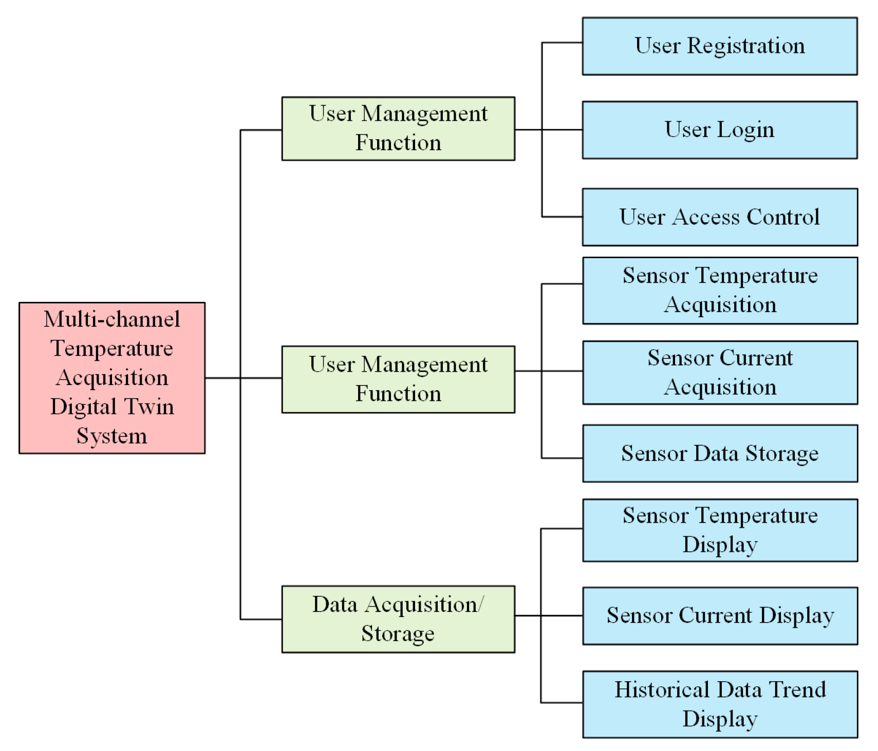
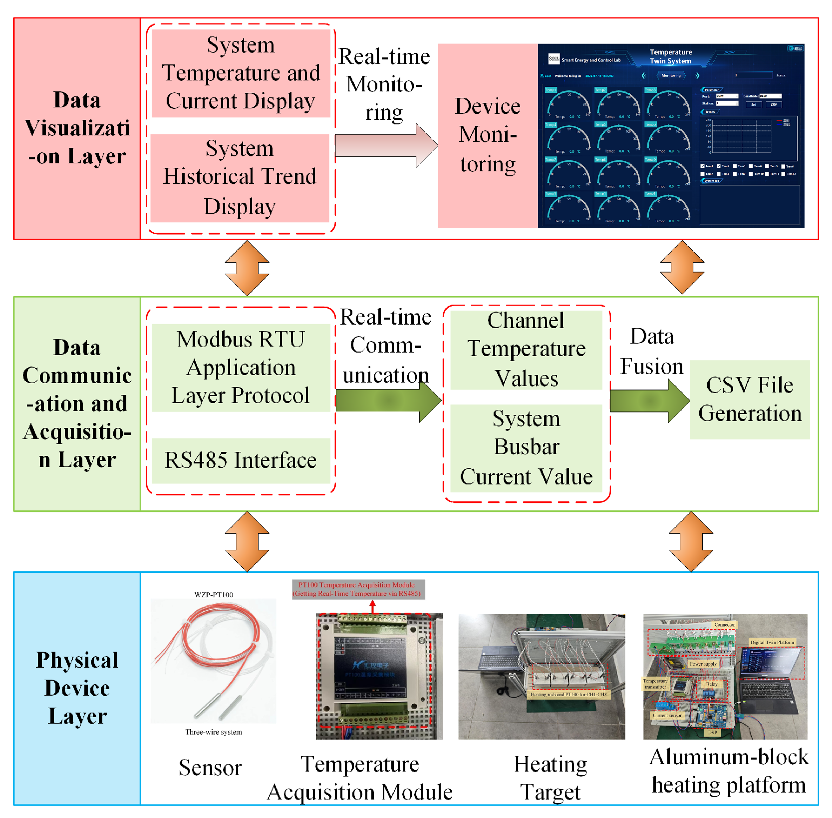
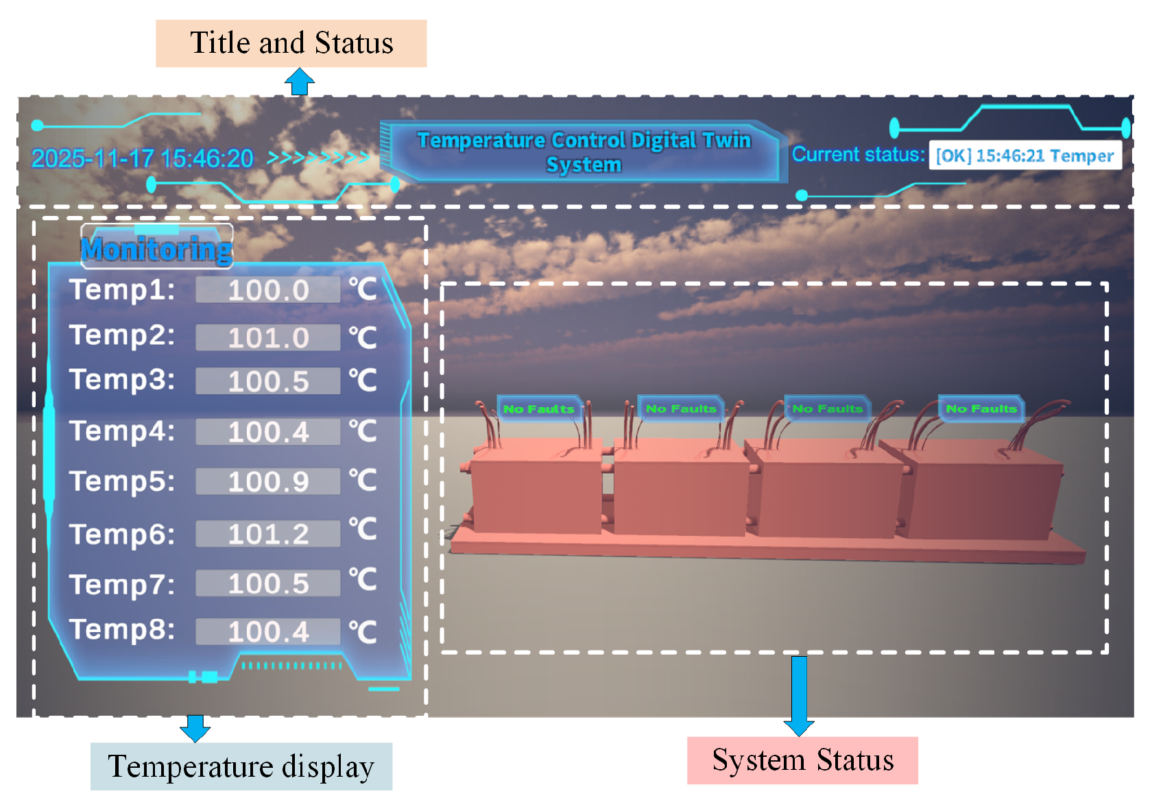
A digital-twin-inspired monitoring framework is developed to synchronize multi-source measurements with a virtual representation, supporting real-time visualization, safe data collection, and offline what-if analysis for intelligent heating processes.

2.

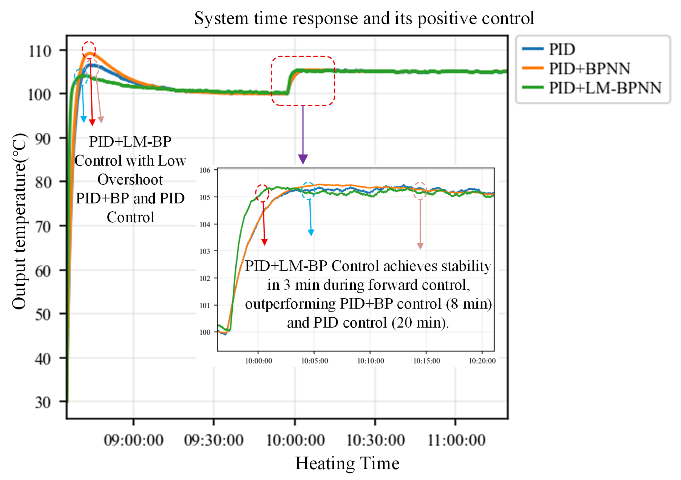
A dynamic interaction strategy combining an LM-optimized BP neural network with conventional tuned PID control is proposed, which enables adaptive online learning and precise temperature regulation in nonlinear, large-time-constant, and large-time-delay multi-point heating systems.

3.

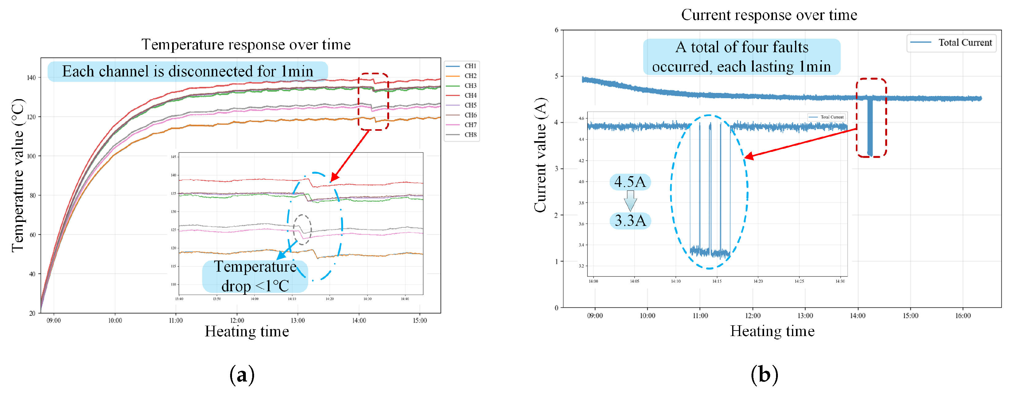
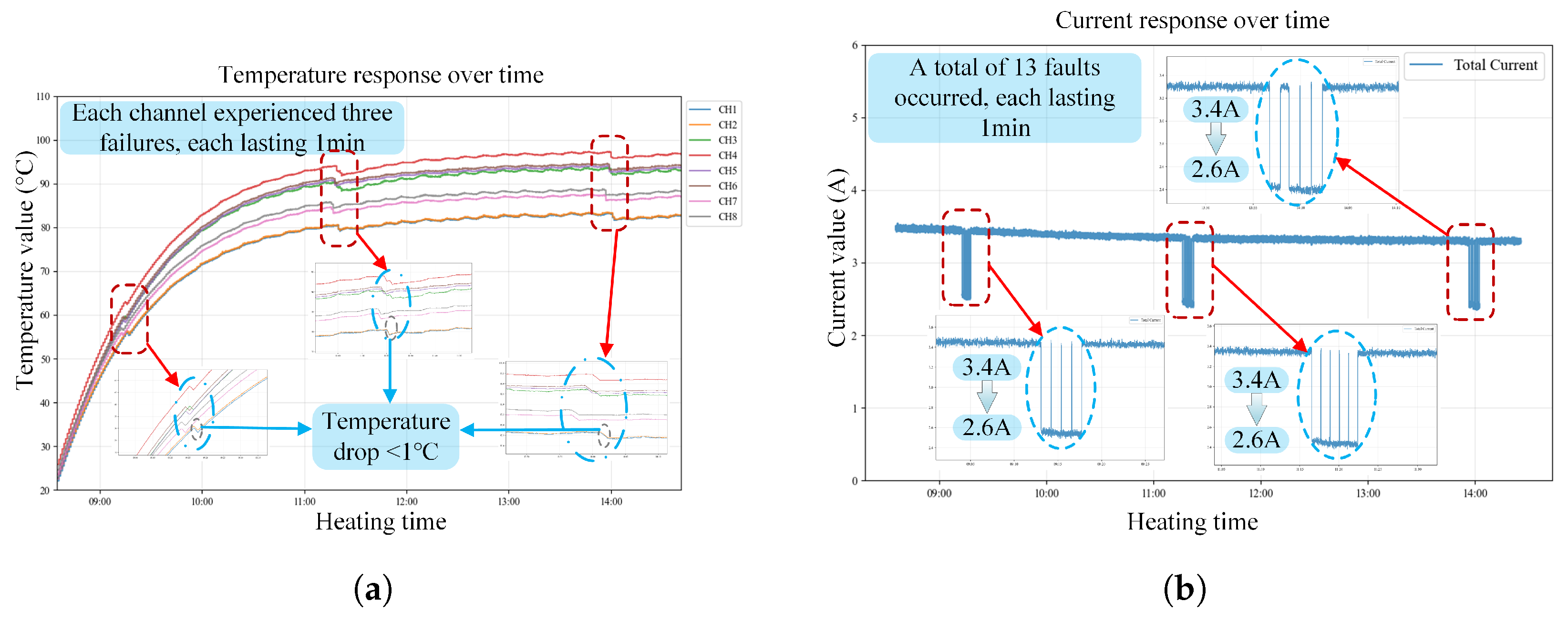
A relay-injected open-circuit fault mechanism and spatiotemporal dataset construction scheme are developed. Using these datasets, a 1D-CNN-based diagnostic model achieves fast detection and channel-level localization of heater open-circuit induced channel anomalies.

The rest of this article is organized as follows. Section 2 and Section 3 provides a detailed introduction to the digital-twin-inspired monitoring system and temperature control algorithms. Section 4 discusses the fault diagnosis methodology and compares it with alternative approaches, while Section 5 presents the simulation setup and experimental validation on the multi-point aluminum block heating platform. Finally, Section 6 concludes this article.

2. Aluminum-Block Heating Platform Design Based on a Digital-Twin-Inspired Monitoring System

Digital-twin-inspired monitoring systems construct a synchronized virtual representation of a physical asset by mapping multi-source measurements into a digital environment in real time. Using sensor data acquisition and cloud computing, information regarding equipment, processes, and operational conditions is synchronized with a digital model, facilitating real-time monitoring and prediction of critical parameters such as temperature, pressure, and vibration. This method integrates sophisticated algorithms for fault diagnosis and dynamic control optimization during unusual operating conditions, thereby enhancing production efficiency and product quality while markedly decreasing energy consumption and maintenance expenses.

2.1. Functional Requirements Analysis of the Digital-Twin-Inspired Monitoring System

To facilitate real-time monitoring of the aluminum-block heating platform, the system must collect and analyze data produced during operation. In this study, the digital twin monitoring system consists of four modules: system management, data acquisition and storage, data visualization, and real-time monitoring. Figure 1 illustrates a functional diagram of the system.

The system management module oversees user registration, following successful identity verification and allocation of role-based permissions, while ensuring the security and compliance of the digital twin platform. The platform collects and stores data by monitoring key parameters in real time, including the temperature of each channel on the aluminum block heating platform and the total equipment current. It preprocesses the raw data and produces standardized CSV files to facilitate subsequent data analysis and interpretation. Data management and real-time monitoring are executed via the ModbusRTU application layer protocol on an RS-485 communication interface. The system dynamically displays real-time data from temperature and current transmitters, intuitively presenting historical trends and current parameters on a visual interface. This allows users to monitor production status with a single button press, thereby enhancing operational efficiency.

2.2. Monitoring System Technical Framework

A three-layer monitoring architecture is established for the aluminum-block heating platform’s visualization system, consisting of the physical device layer, the data communication and acquisition layer, and the data visualization layer. Figure 2 illustrates the technical architecture of the aluminum-block heating platform.

The physical device layer consists of hardware components tasked with real-time data collection, transmission, and preprocessing to guarantee stable system functionality. The data communication and acquisition layer is developed in C# and employs industrial protocols like ModbusRTU to interface with devices, gather real-time data, and produce standardized CSV files for later control and fault diagnosis. The data visualization layer is developed in C# utilizing Windows Forms to exhibit real-time device status, including temperature and current, via dynamic displays and charts, thereby enabling accurate monitoring capabilities. The digital-twin-inspired monitoring platform delineated in this study is illustrated in Figure 3.

3. High-Precision Temperature Control System Based on LM-Optimized BP Neural Network

The digital-twin-inspired monitoring system offers real-time feedback on temperature fluctuations and facilitates the prediction of operational conditions and optimization modifications within a simulated environment. It attains real-time temperature regulation via continuous surveillance and data collection. This study utilizes a BP neural network augmented by the Levenberg–Marquardt algorithm, in conjunction with a PID controller, to attain high-precision temperature control. 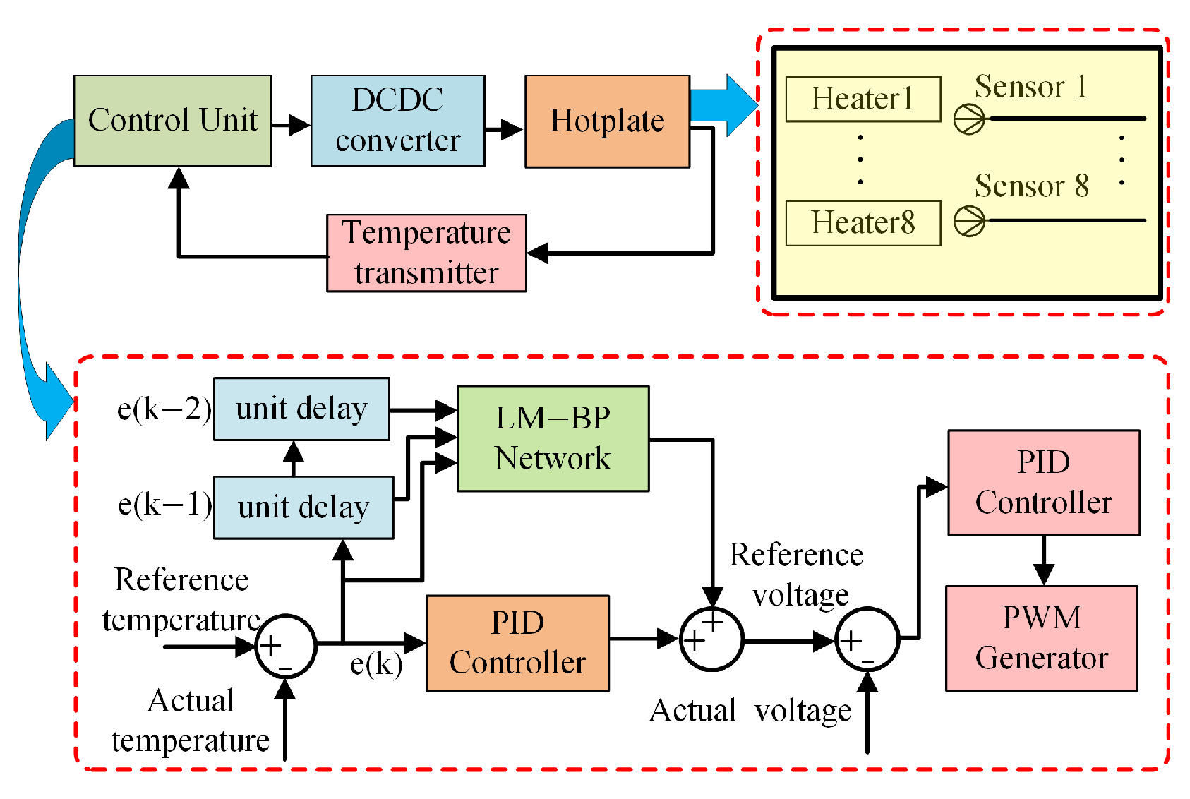Figure 4 illustrates a comprehensive block diagram of the temperature control system for the multi-point aluminum block heating platform.

The complete block diagram of the control system includes a control module, a power-conversion module, and a controlled-object module featuring temperature feedback. The system employs eight low-voltage heating rods to warm the aluminum block. The control scheme utilizes a two-loop strategy, featuring a temperature outer loop and a voltage inner loop. The system gathers real-time temperature data using a three-wire platinum resistance thermometer (RTD) along with a temperature transmitter, compares this data to the setpoint, and produces a target voltage signal through the control algorithm. The target voltage is compared to the measured voltage; the PID controller processes the error and sends it to the PWM generator to create the necessary PWM waveform. The PWM subsequently controls the power switching device to manage the input voltage of the heating rods, thus attaining the desired temperature.

3.1. Controlled Object with Time Delay

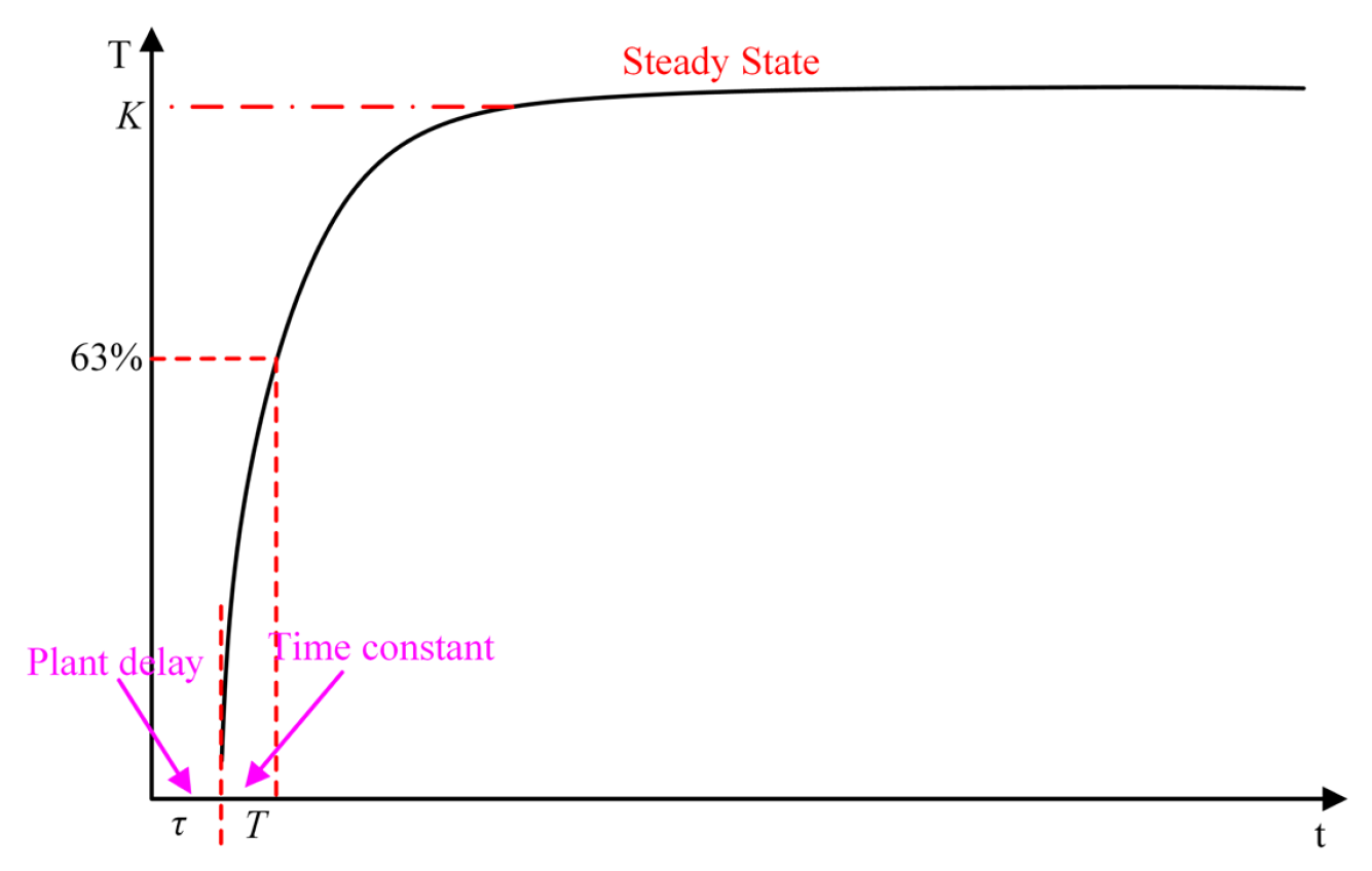
The controlled object is a thermal processing system that can be modeled as a first-order plus time-delay (FOPTD) system. The system’s transfer function is given in Equation (1), where K is the steady-state gain relating output temperature to input current, T is the plant time constant, and $\tau$ is the response delay.

$$P\left(s\right)={\displaystyle \frac{K}{Ts+1}}{e}^{-\tau s}$$

(1)

When a step input of magnitude $I_0$ is applied to the system, the output response is given by Equation (2). The time-domain response $y\left(t\right)$ can be divided into two stages. The first stage is a pure delay, during which the system has not yet begun to respond, and the output remains at its initial value. The second stage is characterized by a first-order rise. After the delay, the output follows a first-order exponential transient and approaches its steady-state value K. The step response of the system is shown in Figure 5.

$$y\left(t\right)=\left\{\begin{array}{cc}0,\hfill & 0\le t<\tau ,\hfill \\ K{I}_0\left[1-e^{-{\displaystyle \frac{t-\tau }{T}}}\right],\hfill & t\ge \tau .\hfill \end{array}\right.$$

(2)

3.2. Traditional PID Control

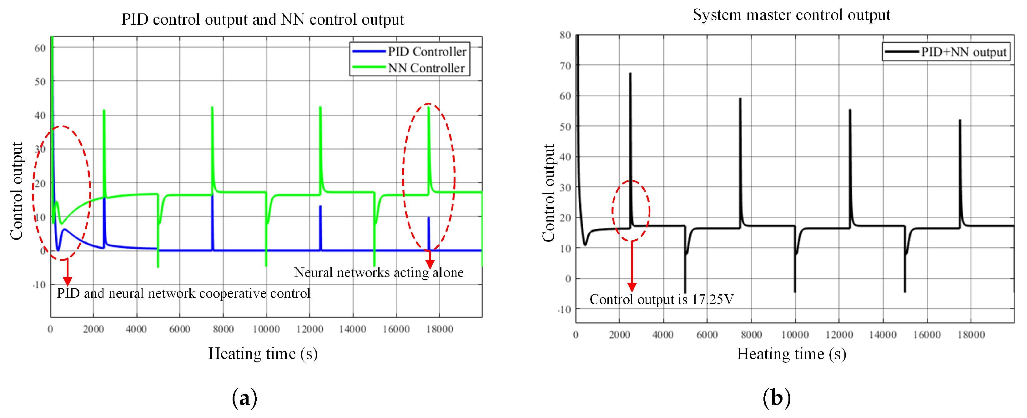
Upon completion of training, the neural network controller assumes the principal control function. During the startup phase, a PID controller regulates the system due to the network’s need for time to learn and stabilize weights. The fundamental PID control law is expressed in Equation (3), where $K_p$ denotes the proportional gain, $T_i$ represents the integral time constant, and $T_d$ signifies the derivative time constant.

$$u\left(t\right)=K_p\left[e\left(t\right)+{\displaystyle \frac{1}{T_i}}{\int }_0^{t}e\left(\tau \right)d\tau +T_d{\displaystyle \frac{de\left(t\right)}{dt}}\right]$$

(3)

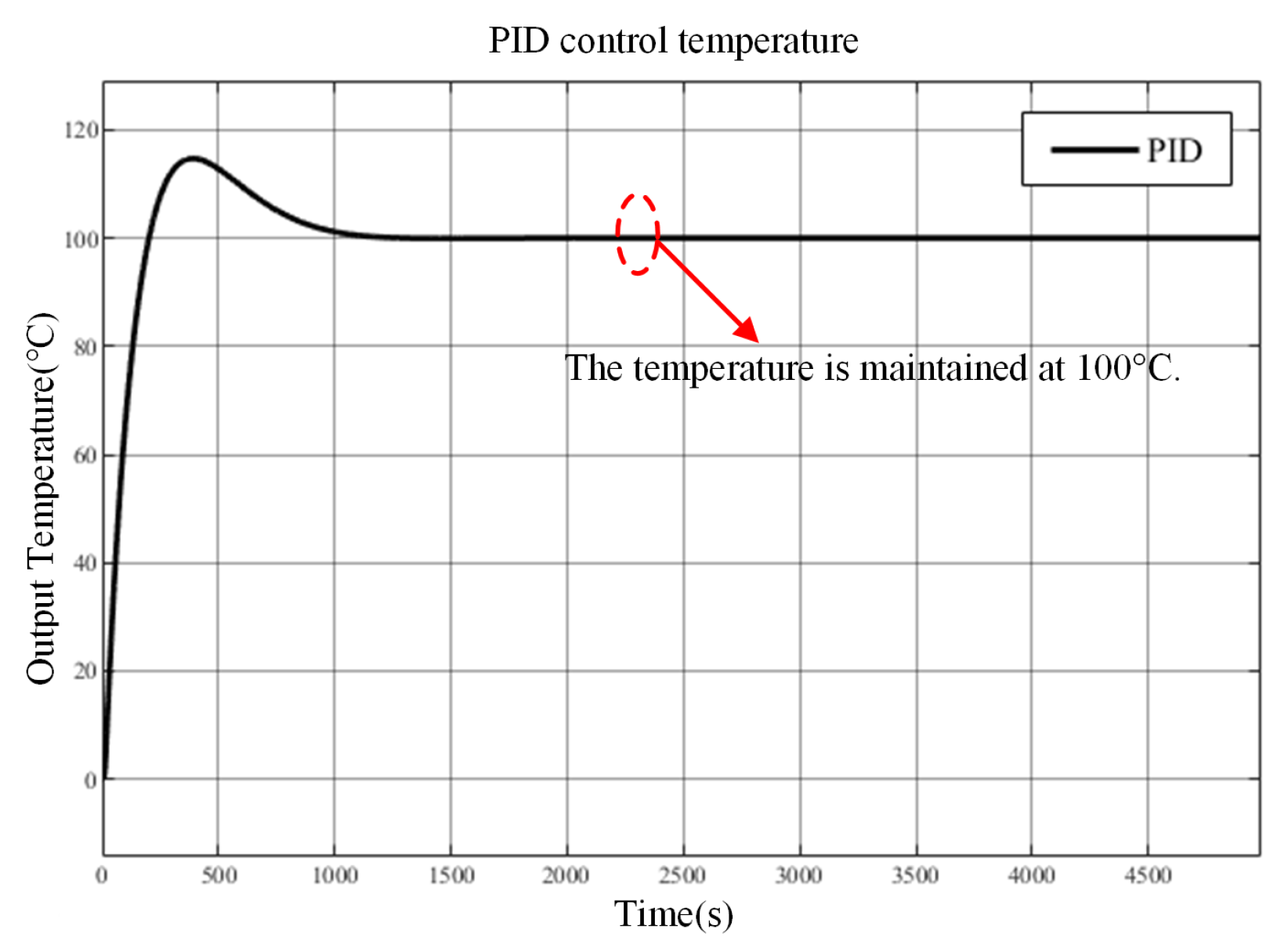
Stability is an essential requirement in control systems. The stability of the PID controller, designed via the step response method, can be assured. The PID parameter values $K_p$, $T_i$, and $T_d$ are derived from $\tau$, K, and T as specified in Equation (1), with their respective formulas presented in Equations (4)–(6). The PID tuning parameters adopted in this study and the key simulation constraints are summarized in

Table 1. PID settings and simulation constraints.

Item	Value
$K_p$	9.74
$T_i$ (s)	1075
$T_d$ (s)	20
Control update period $T_s$ (s)	0.5
Command saturation (V)	$[0,25]$

.

$$K_p=1.2{\displaystyle \frac{T}{\tau }}$$

(4)

$$T_i=0.5T$$

(5)

$$T_d=2\tau$$

(6)

Nonetheless, due to the nonlinearity of the controlled plant and its significant time delay, a PID controller alone results in suboptimal control performance. Consequently, a neural network is implemented to optimize temperature regulation and augment overall control efficacy. In this study, the final control command is obtained by directly adding the outputs of the PID controller and the neural-network controller. At the beginning, the PID output provides a robust baseline, while the neural-network output is continuously refined via Levenberg–Marquardt-based online updating. As the neural network improves its compensation capability and reduces the tracking error, the magnitude of the PID correction required to maintain performance correspondingly decreases over time.

3.3. BP Neural Network

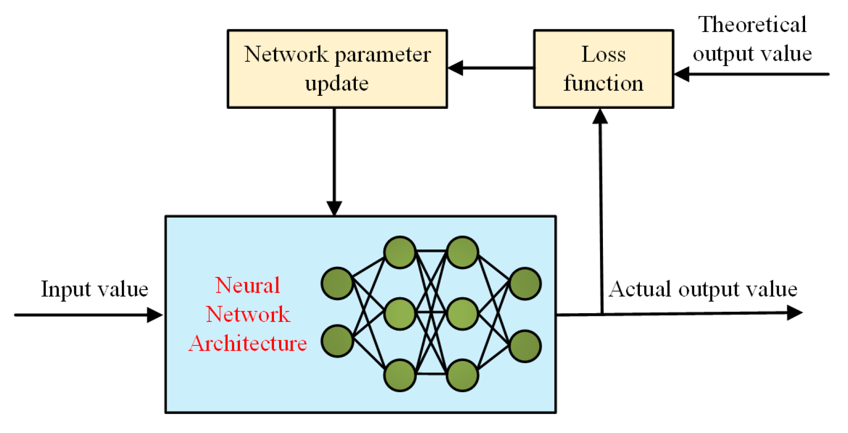
Artificial neural networks (ANNs) are machine learning models that replicate the functions of biological neurons. By emulating the information-processing functions of the human brain, they facilitate modeling and decision-making on intricate datasets. A conventional BP neural network is a standard ANN architecture, typically consisting of an input layer, one or more hidden layers, and an output layer. Neurons convert signals via activation functions. Training generally involves forward propagation, error calculation, and backward propagation. Backpropagation is fundamental to BP networks: gradients of a loss function concerning the network parameters are calculated and utilized with gradient descent to optimize the network. Figure 6 illustrates the fundamental architecture of a BP neural network. These networks can approximate nonlinear relationships. The loss function is derived from the difference between the predicted outputs and the target outputs. The weights and biases are updated to minimize the loss by calculating the partial derivatives of the loss with respect to the parameters.

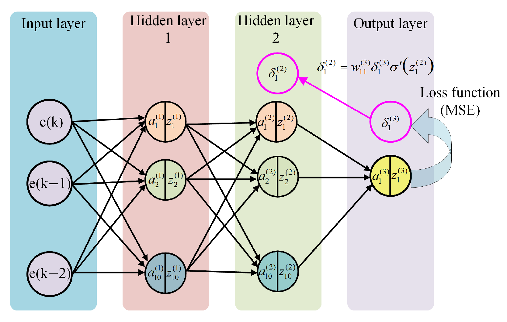
To achieve high-precision temperature control, a multilayer BP neural network is introduced alongside the PID controller. The network architecture, shown in Figure 7, consists of one input layer, two hidden layers, and one output layer; each hidden layer contains 10 neurons. The inputs to the network are the current temperature-tracking error e(k) and the two lagged errors e(k − 1) and e(k − 2), where $y_{ref}$ denotes the temperature setpoint and $y_{out}$ is the measured temperature.

3.3.1. BP Neural Network Forward Propagation

The BP neural network utilizes the error signals e(k), e(k − 1), and e(k − 2) from a conventional PID temperature-control system as inputs, while employing the PID controller output as the target signal. The hidden layers employ the hyperbolic tangent (tanh) activation function, while the output layer is linear. The matrices for weight and bias transitioning from the input layer to the first hidden layer are presented in Equation (7), while the input vector and the formulas for element-wise calculations can be found in Equations (8) and (9). The matrices for weight and bias transitioning from the first hidden layer to the second hidden layer, as well as the formulas for element-wise calculations, are presented in Equations (10) and (11). The weight and bias matrices connecting the second hidden layer to the output layer, as well as the formulas for element-wise calculations, are presented in Equations (12) and (13).

$${\mathbf{W}}^{\left(1\right)}=\left(\begin{array}{ccc}{w}_{11}^{\left(1\right)}& w_{12}^{\left(1\right)}& w_{13}^{\left(1\right)}\\ w_{21}^{\left(1\right)}& w_{22}^{\left(1\right)}& w_{23}^{\left(1\right)}\\ ⋮& ⋮& ⋮\\ w_{n_{1}1}^{\left(1\right)}& w_{n_{1}2}^{\left(1\right)}& w_{n_{1}3}^{\left(1\right)}\end{array}\right),{\mathbf{b}}^{\left(1\right)}=\left(\begin{array}{c}{b}_1^{\left(1\right)}\\ b_2^{\left(1\right)}\\ ⋮\\ b_{n_1}^{\left(1\right)}\end{array}\right).$$

(7)

$$\mathbf{x}=\left(\begin{array}{c}\mathrm{e}\left(\mathrm{k}\right)\\ \mathrm{e}(\mathrm{k}-\mathbf{1})\\ \mathrm{e}(\mathrm{k}-\mathbf{2})\end{array}\right)$$

(8)

$$\begin{array}{c}{\mathbf{z}}^{\left(1\right)}=f^{\left(1\right)}({\mathbf{W}}^{\left(1\right)}\mathbf{x}+{\mathbf{b}}^{\left(1\right)})=f^{\left(1\right)}\left(\begin{array}{c}{\displaystyle \sum _{j=1}^3}{w}_{1j}^{\left(1\right)}{x}_j+b_1^{\left(1\right)}\\ {\displaystyle \sum _{j=1}^3}{w}_{2j}^{\left(1\right)}{x}_j+b_2^{\left(1\right)}\\ ⋮\\ {\displaystyle \sum _{j=1}^3}{w}_{n_{1}j}^{\left(1\right)}{x}_j+b_{n_1}^{\left(1\right)}\end{array}\right)\hfill \end{array}$$

(9)

$${\mathbf{W}}^{\left(2\right)}=\left(\begin{array}{cccc}{w}_{11}^{\left(2\right)}& w_{12}^{\left(2\right)}& \dots & w_{1n_1}^{\left(2\right)}\\ w_{21}^{\left(2\right)}& w_{22}^{\left(2\right)}& \dots & w_{2n_1}^{\left(2\right)}\\ ⋮& ⋮& \ddots & ⋮\\ w_{n_{2}1}^{\left(2\right)}& w_{n_{2}2}^{\left(2\right)}& \dots & w_{n_2{n}_1}^{\left(2\right)}\end{array}\right),{\mathbf{b}}^{\left(2\right)}=\left(\begin{array}{c}{b}_1^{\left(2\right)}\\ b_2^{\left(2\right)}\\ ⋮\\ b_{n_2}^{\left(2\right)}\end{array}\right)$$

(10)

$$\begin{array}{c}{\mathbf{z}}^{\left(2\right)}=f^{\left(2\right)}({\mathbf{W}}^{\left(2\right)}{\mathbf{z}}^{\left(1\right)}+{\mathbf{b}}^{\left(2\right)})=f^{\left(2\right)}\left(\begin{array}{c}{\displaystyle \sum _{i=1}^{n_1}}{w}_{1i}^{\left(2\right)}{z}_i^{\left(1\right)}+b_1^{\left(2\right)}\\ {\displaystyle \sum _{i=1}^{n_1}}{w}_{2i}^{\left(2\right)}{z}_i^{\left(1\right)}+b_2^{\left(2\right)}\\ ⋮\\ {\displaystyle \sum _{i=1}^{n_1}}{w}_{n_{2}i}^{\left(2\right)}{z}_i^{\left(1\right)}+b_{n_2}^{\left(2\right)}\end{array}\right)\hfill \end{array}$$

(11)

$${\mathbf{W}}^{\left(3\right)}=(w_1^{\left(3\right)},w_2^{\left(3\right)},\dots ,w_{n_2}^{\left(3\right)}),{\mathbf{b}}^{\left(3\right)}$$

(12)

$$\begin{array}{c}\widehat{y}={\mathbf{a}}^{\left(3\right)}=f^{\left(3\right)}\left({\mathbf{z}}^{\left(3\right)}\right)={\mathbf{z}}^{\left(3\right)}={\mathbf{W}}^{\left(3\right)}{\mathbf{z}}^{\left(2\right)}+{\mathbf{b}}^{\left(3\right)}={\displaystyle \sum _{i=1}^{n_2}}{w}_i^{\left(3\right)}{z}_i^{\left(2\right)}+b^{\left(3\right)}\hfill \end{array}$$

(13)

In these expressions, ${\mathbf{W}}^{\left(1\right)}$, ${\mathbf{W}}^{\left(2\right)}$, and ${\mathbf{W}}^{\left(3\right)}$ denote the weight matrices for layers 1–3, and ${\mathbf{b}}^{\left(1\right)}$, ${\mathbf{b}}^{\left(2\right)}$, and ${\mathbf{b}}^{\left(3\right)}$ denote the corresponding bias vectors. Specifically, the BP network consists of an input layer, two hidden layers, and an output layer. Let $n_0$ be the input dimension, and let $n_1$ and $n_2$ be the numbers of neurons in the first and second hidden layers, respectively. Then, ${\mathbf{W}}^{\left(1\right)}\in {\mathbf{R}}^{n_1\times n_0}$ and ${\mathbf{b}}^{\left(1\right)}\in {\mathbf{R}}^{n_1}$ map the input layer to the first hidden layer, ${\mathbf{W}}^{\left(2\right)}\in {\mathbf{R}}^{n_2\times n_1}$ and ${\mathbf{b}}^{\left(2\right)}\in {\mathbf{R}}^{n_2}$ map the first hidden layer to the second hidden layer, and ${\mathbf{W}}^{\left(3\right)}\in {\mathbf{R}}^{1\times n_2}$ and ${\mathbf{b}}^{\left(3\right)}\in \mathbf{R}$ map the second hidden layer to the output layer. The element $w_{ij}^{\left(l\right)}$ denotes the weight connecting the j-th neuron in layer $l-1$ to the i-th neuron in layer l, and $b_i^{\left(l\right)}$ denotes the bias of the i-th neuron in layer l.

The activation functions $f^{\left(1\right)}$ and $f^{\left(2\right)}$ are hyperbolic tangent (tanh) functions with an output range of $(-1,1)$, which introduce nonlinearity and improve the representation capability of the hidden layers. The output-layer activation $f^{\left(3\right)}$ is chosen as a linear function to produce an unconstrained real-valued output, which is suitable for regression and helps prevent output saturation, thereby facilitating stable gradient-based training during backpropagation.

3.3.2. BP Neural Network Error Calculation

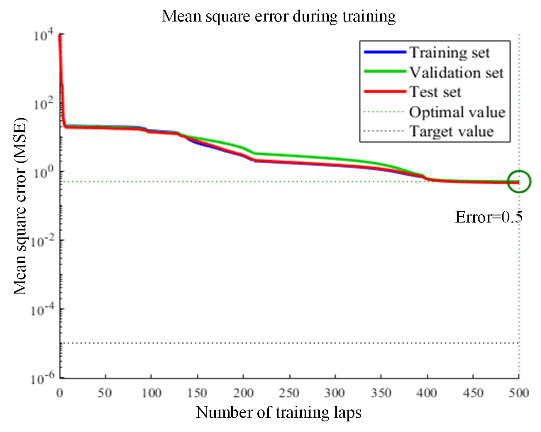
For nonlinear regression problems, neural networks typically use the mean squared error (MSE) as the loss function. For the k-th sample with target $y^{\left(k\right)}$ and predicted output ${\widehat{y}}^{\left(k\right)}$, the sample error and the mean squared error are defined in Equations (14) and (15).

$$e^{\left(\mathrm{k}\right)}={\widehat{y}}^{\left(\mathrm{k}\right)}-y^{\left(\mathrm{k}\right)}$$

(14)

$$E={\displaystyle \frac{1}{N}}\sum _{k=1}^N{\left(e^{\left(\mathrm{k}\right)}\right)}^2$$

(15)

In these expressions, $e\left(k\right)$ denotes the error between the target and predicted outputs, and E denotes the mean squared error. For a dataset with N samples, the overall loss is given in Equation (16).

$$L={\displaystyle \frac{1}{N}}\sum _{n=1}^N{\displaystyle \frac{1}{2}}{\left({\widehat{y}}^{\left(n\right)}-y^{\left(n\right)}\right)}^2$$

(16)

In this expression, L denotes the overall loss of the prediction model, N is the number of samples, $y^{\left(n\right)}$ and ${\widehat{y}}^{\left(n\right)}$ denote the true value and the predicted value of the nth sample, respectively.

3.3.3. Backpropagation in BP Neural Networks

Backpropagation calculates the gradients of the loss concerning the parameters using the chain rule, transmitting error signals from the output layer of the BP neural network controller back to the input layer. The network has been optimized through the use of gradient descent. For every sample and each layer, the error terms and parameter gradients are calculated to establish the update direction; using a learning rate $\eta$, the weights and biases are adjusted accordingly. The gradient for the output layer with a linear activation is derived directly using the chain rule, streamlining the computation process.

The error term ${\mathsf{\delta }}^{\left(3\right)}$, the weight gradient ${\displaystyle \frac{\partial \mathbf{E}}{\partial {\mathbf{W}}^{\left(3\right)}}}$, and the bias gradient ${\displaystyle \frac{\partial \mathbf{E}}{\partial {\mathbf{b}}^{\left(3\right)}}}$ are given by Equations (17)–(19).

$${\mathsf{\delta }}^{\left(3\right)}={\displaystyle \frac{\partial \mathbf{E}}{\partial {\mathbf{z}}^{\left(3\right)}}}={\displaystyle \frac{\partial \mathbf{E}}{\partial \widehat{\mathbf{y}}}}·{\displaystyle \frac{\partial \widehat{\mathbf{y}}}{\partial {\mathbf{z}}^{\left(3\right)}}}={\displaystyle \frac{\partial \mathbf{E}}{\partial {\mathsf{\delta }}^{\left(2\right)}}}=\left(\begin{array}{c}{\displaystyle \frac{\partial E}{\partial {\delta }_1^{\left(2\right)}}}\\ {\displaystyle \frac{\partial E}{\partial {\delta }_2^{\left(2\right)}}}\\ ⋮\\ {\displaystyle \frac{\partial E}{\partial {\delta }_{n_1}^{\left(2\right)}}}\end{array}\right)=\left(\begin{array}{c}{\widehat{y}}_1-y_1\\ {\widehat{y}}_2-y_2\\ ⋮\\ {\widehat{y}}_{n_1}-y_{n_1}\end{array}\right)$$

(17)

$$\begin{array}{c}{\displaystyle \frac{\partial \mathbf{E}}{\partial {\mathbf{W}}^{\left(3\right)}}}={\displaystyle \frac{\partial \mathbf{E}}{\partial {\mathbf{z}}^{\left(3\right)}}}·{\displaystyle \frac{\partial {\mathbf{z}}^{\left(3\right)}}{\partial {\mathbf{W}}^{\left(3\right)}}}={\mathsf{\delta }}^{\left(3\right)}\times {\left({\mathbf{a}}^{\left(2\right)}\right)}^{\top }=\left(\begin{array}{cccc}{\delta }_1^{\left(3\right)}{a}_1^{\left(2\right)}& {\delta }_1^{\left(3\right)}{a}_2^{\left(2\right)}& \dots & {\delta }_1^{\left(3\right)}{a}_{n_1}^{\left(2\right)}\\ {\delta }_2^{\left(3\right)}{a}_1^{\left(2\right)}& {\delta }_2^{\left(3\right)}{a}_2^{\left(2\right)}& \dots & {\delta }_2^{\left(3\right)}{a}_{n_1}^{\left(2\right)}\\ ⋮& ⋮& \ddots & ⋮\\ {\delta }_{n_2}^{\left(3\right)}{a}_1^{\left(2\right)}& {\delta }_{n_2}^{\left(3\right)}{a}_2^{\left(2\right)}& \dots & {\delta }_{n_2}^{\left(3\right)}{a}_{n_1}^{\left(2\right)}\end{array}\right)\hfill \end{array}$$

(18)

$${\displaystyle \frac{\partial \mathbf{E}}{\partial {\mathbf{b}}^{\left(3\right)}}}={\displaystyle \frac{\partial \mathbf{E}}{\partial {\mathbf{z}}^{\left(3\right)}}}·{\displaystyle \frac{\partial {\mathbf{z}}^{\left(3\right)}}{\partial {\mathbf{b}}^{\left(3\right)}}}={\displaystyle \frac{\partial \mathbf{E}}{\partial {\mathbf{b}}^{\left(3\right)}}}=\left(\begin{array}{c}{\displaystyle \frac{\partial E}{\partial b_1^{\left(3\right)}}}\\ {\displaystyle \frac{\partial E}{\partial b_2^{\left(3\right)}}}\\ ⋮\\ {\displaystyle \frac{\partial E}{\partial b_n^{\left(3\right)}}}\end{array}\right)=\left(\begin{array}{c}{\delta }_1^{\left(3\right)}\\ {\delta }_2^{\left(3\right)}\\ ⋮\\ {\delta }_n^{\left(3\right)}\end{array}\right)$$

(19)

Both the activation functions of the first and second hidden layers are the hyperbolic tangent (tanh); the corresponding formulas for the error, weight gradients, and bias gradients are given in Equations (20)–(25).

$$\begin{array}{c}{\mathsf{\delta }}^{\left(2\right)}={\left({\mathbf{W}}^{\left(3\right)}\right)}^{\top }·{\mathsf{\delta }}^{\left(3\right)}\times {\sigma }^{\prime }\left({\mathbf{z}}^{\left(2\right)}\right)=\left(\begin{array}{ccc}{w}_{11}^{\left(3\right)}& \dots & w_{1n}^{\left(3\right)}\\ ⋮& \ddots & ⋮\\ w_{n1}^{\left(3\right)}& \dots & w_{nn}^{\left(3\right)}\end{array}\right)\left(\begin{array}{c}{\delta }_1^{\left(3\right)}\\ ⋮\\ {\delta }_n^{\left(3\right)}\end{array}\right)\left(\begin{array}{c}{\sigma }^{\prime }\left(z_1^{\left(2\right)}\right)\\ ⋮\\ {\sigma }^{\prime }\left(z_{n_1}^{\left(2\right)}\right)\end{array}\right)\\ =\left(\begin{array}{c}{\displaystyle \sum _{k=1}^n}{w}_{k1}^{\left(3\right)}{\delta }_k^{\left(3\right)}\\ ⋮\\ {\displaystyle \sum _{k=1}^n}{w}_{k{n}_1}^{\left(3\right)}{\delta }_k^{\left(3\right)}\end{array}\right)\left(\begin{array}{c}{\sigma }^{\prime }\left(z_1^{\left(2\right)}\right)\\ ⋮\\ {\sigma }^{\prime }\left(z_{n_1}^{\left(2\right)}\right)\end{array}\right)=\left(\begin{array}{c}\left({\displaystyle \sum _{k=1}^n}{w}_{1k}^{\left(3\right)}{\delta }_k^{\left(3\right)}\right){\sigma }^{\prime }\left(z_1^{\left(2\right)}\right)\\ ⋮\\ \left({\displaystyle \sum _{k=1}^n}{w}_{n_{1}k}^{\left(3\right)}{\delta }_k^{\left(3\right)}\right){\sigma }^{\prime }\left(z_{n_1}^{\left(2\right)}\right)\end{array}\right)\end{array}$$

(20)

$$\begin{array}{c}{\mathsf{\delta }}^{\left(1\right)}={\mathsf{\delta }}^{\left(2\right)}·{\mathbf{W}}^{\left(2\right)}\times {\sigma }^{\prime }\left({\mathbf{z}}^{\left(1\right)}\right)=\left(\begin{array}{ccc}{w}_{11}^{\left(2\right)}& \dots & w_{1n}^{\left(2\right)}\\ ⋮& \ddots & ⋮\\ w_{n1}^{\left(2\right)}& \dots & w_{nn}^{\left(2\right)}\end{array}\right)\left(\begin{array}{c}{\delta }_1^{\left(2\right)}\\ ⋮\\ {\delta }_n^{\left(2\right)}\end{array}\right)\left(\begin{array}{c}{\sigma }^{\prime }\left(z_1^{\left(1\right)}\right)\\ ⋮\\ {\sigma }^{\prime }\left(z_{n_1}^{\left(1\right)}\right)\end{array}\right)\\ =\left(\begin{array}{c}{\displaystyle \sum _{k=1}^n}{w}_{k1}^{\left(2\right)}{\delta }_k^{\left(2\right)}\\ ⋮\\ {\displaystyle \sum _{k=1}^n}{w}_{k{n}_1}^{\left(2\right)}{\delta }_k^{\left(2\right)}\end{array}\right)\left(\begin{array}{c}{\sigma }^{\prime }\left(z_1^{\left(1\right)}\right)\\ ⋮\\ {\sigma }^{\prime }\left(z_{n_1}^{\left(1\right)}\right)\end{array}\right)=\left(\begin{array}{c}\left({\displaystyle \sum _{k=1}^n}{w}_{1k}^{\left(2\right)}{\delta }_k^{\left(2\right)}\right){\sigma }^{\prime }\left(z_1^{\left(1\right)}\right)\\ ⋮\\ \left({\displaystyle \sum _{k=1}^n}{w}_{n_{1}k}^{\left(2\right)}{\delta }_k^{\left(2\right)}\right){\sigma }^{\prime }\left(z_{n_1}^{\left(1\right)}\right)\end{array}\right)\end{array}$$

(21)

$$\begin{array}{c}{\displaystyle \frac{\partial \mathbf{E}}{\partial {\mathbf{W}}^{\left(2\right)}}}={\displaystyle \frac{\partial \mathbf{E}}{\partial {\mathbf{z}}^{\left(2\right)}}}·{\displaystyle \frac{\partial {\mathbf{z}}^{\left(2\right)}}{\partial {\mathbf{W}}^{\left(2\right)}}}={\mathsf{\delta }}^{\left(2\right)}\times {\left({\mathbf{a}}^{\left(1\right)}\right)}^{\top }=\left(\begin{array}{cccc}{\delta }_1^{\left(2\right)}{a}_1^{\left(1\right)}& {\delta }_1^{\left(2\right)}{a}_2^{\left(1\right)}& \dots & {\delta }_1^{\left(2\right)}{a}_n^{\left(1\right)}\\ {\delta }_2^{\left(2\right)}{a}_1^{\left(1\right)}& {\delta }_2^{\left(2\right)}{a}_2^{\left(1\right)}& \dots & {\delta }_2^{\left(2\right)}{a}_n^{\left(1\right)}\\ ⋮& ⋮& \ddots & ⋮\\ {\delta }_m^{\left(2\right)}{a}_1^{\left(1\right)}& {\delta }_m^{\left(2\right)}{a}_2^{\left(1\right)}& \dots & {\delta }_m^{\left(2\right)}{a}_n^{\left(1\right)}\end{array}\right)\hfill \end{array}$$

(22)

$${\displaystyle \frac{\partial \mathbf{E}}{\partial {\mathbf{b}}^{\left(2\right)}}}={\displaystyle \frac{\partial \mathbf{E}}{\partial {\mathbf{z}}^{\left(2\right)}}}·{\displaystyle \frac{\partial {\mathbf{z}}^{\left(2\right)}}{\partial {\mathbf{b}}^{\left(2\right)}}}=\left(\begin{array}{c}{\displaystyle \frac{\partial E}{\partial b_1^{\left(2\right)}}}\\ {\displaystyle \frac{\partial E}{\partial b_2^{\left(2\right)}}}\\ ⋮\\ {\displaystyle \frac{\partial E}{\partial b_n^{\left(2\right)}}}\end{array}\right)=\left(\begin{array}{c}{\delta }_1^{\left(2\right)}\\ {\delta }_2^{\left(2\right)}\\ ⋮\\ {\delta }_n^{\left(2\right)}\end{array}\right)$$

(23)

$$\begin{array}{c}{\displaystyle \frac{\partial \mathbf{E}}{\partial {\mathbf{W}}^{\left(1\right)}}}={\displaystyle \frac{\partial \mathbf{E}}{\partial {\mathbf{z}}^{\left(1\right)}}}·{\displaystyle \frac{\partial {\mathbf{z}}^{\left(1\right)}}{\partial {\mathbf{W}}^{\left(1\right)}}}={\mathsf{\delta }}^{\left(1\right)}\times {\mathbf{x}}^{\top }=\left(\begin{array}{cccc}{\delta }_1^{\left(1\right)}{x}_1& {\delta }_1^{\left(1\right)}{x}_2& \dots & {\delta }_1^{\left(1\right)}{x}_n\\ {\delta }_2^{\left(1\right)}{x}_1& {\delta }_2^{\left(1\right)}{x}_2& \dots & {\delta }_2^{\left(1\right)}{x}_n\\ ⋮& ⋮& \ddots & ⋮\\ {\delta }_m^{\left(1\right)}{x}_1& {\delta }_m^{\left(1\right)}{x}_2& \dots & {\delta }_m^{\left(1\right)}{x}_n\end{array}\right)\hfill \end{array}$$

(24)

$${\displaystyle \frac{\partial \mathbf{E}}{\partial {\mathbf{b}}^{\left(1\right)}}}={\displaystyle \frac{\partial \mathbf{E}}{\partial {\mathbf{z}}^{\left(1\right)}}}·{\displaystyle \frac{\partial {\mathbf{z}}^{\left(1\right)}}{\partial {\mathbf{b}}^{\left(1\right)}}}=\left(\begin{array}{c}{\displaystyle \frac{\partial E}{\partial b_1^{\left(1\right)}}}\\ {\displaystyle \frac{\partial E}{\partial b_2^{\left(1\right)}}}\\ ⋮\\ {\displaystyle \frac{\partial E}{\partial b_n^{\left(1\right)}}}\end{array}\right)=\left(\begin{array}{c}{\delta }_1^{\left(1\right)}\\ {\delta }_2^{\left(1\right)}\\ ⋮\\ {\delta }_n^{\left(1\right)}\end{array}\right)$$

(25)

In these expressions, the error terms for the second and first hidden layers are denoted by ${\mathsf{\delta }}^{\left(2\right)}$ and ${\mathsf{\delta }}^{\left(1\right)}$, respectively; the corresponding weight and bias gradients are ${\displaystyle \frac{\partial E}{\partial {\mathbf{W}}^{\left(2\right)}}}$ and ${\displaystyle \frac{\partial E}{\partial {\mathbf{b}}^{\left(2\right)}}}$ for the second hidden layer, and ${\displaystyle \frac{\partial E}{\partial {\mathbf{W}}^{\left(1\right)}}}$ and ${\displaystyle \frac{\partial E}{\partial {\mathbf{b}}^{\left(1\right)}}}$ for the first hidden layer. After obtaining the gradients for each layer, the parameters can be updated. The update formulas for weights and biases are given in Equations (26) and (27).

$$\mathbf{w}\leftarrow \mathbf{w}-\eta {\displaystyle \frac{\partial \mathbf{E}}{\partial \mathbf{w}}}$$

(26)

$$\mathbf{b}\leftarrow \mathbf{b}-\eta {\displaystyle \frac{\partial \mathbf{E}}{\partial \mathbf{b}}}$$

(27)

Through repeated iterations of this process, the neural network progressively adjusts all network weights and biases on the given training data, thereby minimizing the mean squared error (MSE) and completing the regression fit.

3.4. BP Neural Network Improved by the Levenberg–Marquardt (LM) Algorithm

Conventional backpropagation (BP) neural networks utilize solely first-order information in the optimization process. To achieve a more rapid and stable minimization method, second-order information (the Hessian) may be integrated. Nevertheless, due to the elevated dimensionality and computational expense, explicitly constructing the Hessian and resolving the corresponding Newton system are unfeasible for neural networks. The Gauss–Newton (GN) approximation of the Hessian is utilized to resolve this issue. The resultant approximation is presented in Equation (28).

$$\begin{array}{c}\mathrm{H}\approx {\mathrm{J}}^{\top }\mathrm{J}=\left(\begin{array}{cccc}{\displaystyle \sum _{i=1}^m}{\left({\displaystyle \frac{\partial f_i}{\partial w_1}}\right)}^2& {\displaystyle \sum _{i=1}^m}{\displaystyle \frac{\partial f_i}{\partial w_1}}{\displaystyle \frac{\partial f_i}{\partial w_2}}& \dots & {\displaystyle \sum _{i=1}^m}{\displaystyle \frac{\partial f_i}{\partial w_1}}{\displaystyle \frac{\partial f_i}{\partial w_n}}\\ {\displaystyle \sum _{i=1}^m}{\displaystyle \frac{\partial f_i}{\partial w_2}}{\displaystyle \frac{\partial f_i}{\partial w_1}}& {\displaystyle \sum _{i=1}^m}{\left({\displaystyle \frac{\partial f_i}{\partial w_2}}\right)}^2& \dots & {\displaystyle \sum _{i=1}^m}{\displaystyle \frac{\partial f_i}{\partial w_2}}{\displaystyle \frac{\partial f_i}{\partial w_n}}\\ ⋮& ⋮& \ddots & ⋮\\ {\displaystyle \sum _{i=1}^m}{\displaystyle \frac{\partial f_i}{\partial w_n}}{\displaystyle \frac{\partial f_i}{\partial w_1}}& {\displaystyle \sum _{i=1}^m}{\displaystyle \frac{\partial f_i}{\partial w_n}}{\displaystyle \frac{\partial f_i}{\partial w_2}}& \dots & {\displaystyle \sum _{i=1}^m}{\left({\displaystyle \frac{\partial f_i}{\partial w_n}}\right)}^2\end{array}\right)\hfill \end{array}$$

(28)

In this expression, $\mathrm{J}$ denotes the Jacobian matrix. With this approximation, second-order derivatives need not be computed; instead, all gradients can be obtained in a single backpropagation, enabling construction of $\mathrm{J}$ and approximation of the Hessian. On this basis, the standard Gauss–Newton step is given in Equation (29).

$$\Delta \mathbf{w}=-{\left({\mathbf{J}}^{\top }\mathbf{J}\right)}^{-\mathbf{1}}{\mathbf{J}}^{\top }\mathbf{e}=-\left(\begin{array}{cccc}{\left({\mathbf{J}}^{\top }\mathbf{J}\right)}_{\mathbf{11}}^{-\mathbf{1}}& {\left({\mathbf{J}}^{\top }\mathbf{J}\right)}_{\mathbf{12}}^{-\mathbf{1}}& \dots & {\left({\mathbf{J}}^{\top }\mathbf{J}\right)}_{\mathbf{1}\mathbf{n}}^{-\mathbf{1}}\\ {\left({\mathbf{J}}^{\top }\mathbf{J}\right)}_{\mathbf{21}}^{-\mathbf{1}}& {\left({\mathbf{J}}^{\top }\mathbf{J}\right)}_{\mathbf{22}}^{-\mathbf{1}}& \dots & {\left({\mathbf{J}}^{\top }\mathbf{J}\right)}_{\mathbf{2}\mathbf{n}}^{-\mathbf{1}}\\ ⋮& ⋮& \ddots & ⋮\\ {\left({\mathbf{J}}^{\top }\mathbf{J}\right)}_{\mathbf{n}\mathbf{1}}^{-\mathbf{1}}& {\left({\mathbf{J}}^{\top }\mathbf{J}\right)}_{\mathbf{n}\mathbf{2}}^{-\mathbf{1}}& \dots & {\left({\mathbf{J}}^{\top }\mathbf{J}\right)}_{\mathbf{nn}}^{-\mathbf{1}}\end{array}\right)\left(\begin{array}{c}{\displaystyle \sum _{\mathbf{k}=\mathbf{1}}^{\mathbf{m}}}{\displaystyle \frac{\partial {\mathbf{e}}_{\mathbf{k}}}{\partial {\mathbf{w}}_{\mathbf{1}}}}{\mathbf{e}}_{\mathbf{k}}\\ {\displaystyle \sum _{\mathbf{k}=\mathbf{1}}^{\mathbf{m}}}{\displaystyle \frac{\partial {\mathbf{e}}_{\mathbf{k}}}{\partial {\mathbf{w}}_{\mathbf{2}}}}{\mathbf{e}}_{\mathbf{k}}\\ ⋮\\ {\displaystyle \sum _{\mathbf{k}=\mathbf{1}}^{\mathbf{m}}}{\displaystyle \frac{\partial {\mathbf{e}}_{\mathbf{k}}}{\partial {\mathbf{w}}_{\mathbf{n}}}}{\mathbf{e}}_{\mathbf{k}}\end{array}\right)$$

(29)

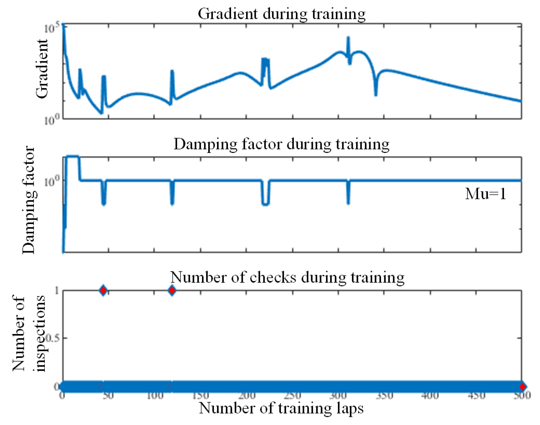
The Gauss–Newton method utilizes an approximate second-order framework that generally converges more rapidly than standard gradient descent; however, the corresponding normal matrix is not assured to be strictly positive definite, which may result in the existence of ${\left({\mathbf{J}}^{\top }\mathbf{J}\right)}^{-1}$, rendering the method susceptible to noise. The Levenberg–Marquardt (LM) algorithm enhances the Gauss–Newton method by incorporating a damping factor and appending a scaled identity matrix to the Hessian approximation ${\mathbf{J}}^{\top }\mathbf{J}$. This modification alleviates the deficiencies of Gauss–Newton and facilitates more dependable parameter updates. The update step is delineated in Equation (30).

$$\Delta \mathbf{W}=-{({\mathbf{J}}^{\top }\mathbf{J}+\mu \mathbf{I})}^{-1}{\mathbf{J}}^{\top }e$$

(30)

In this expression, $\mathbf{I}$ denotes the identity matrix and $\mu$ the damping factor. When $\mu$ is large, the parameter updates are equivalent to those of the standard gradient descent algorithm; when $\mu$ is small, the updates reduce to the Gauss–Newton (GN) algorithm, yielding fast second-order convergence.

4. Breakpoint Fault Diagnosis Based on a Digital Twin Aluminum-Block Heating Platform

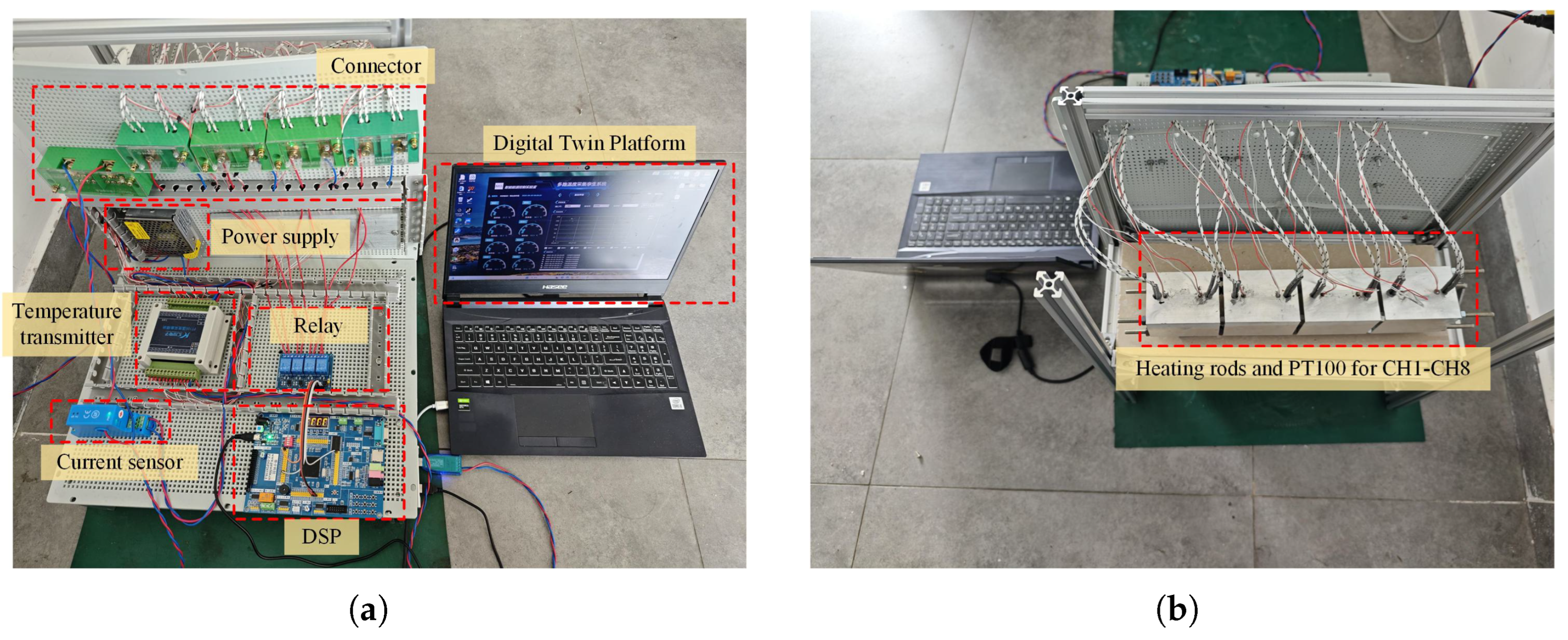
The heating system of the aluminum-block heating platform, being a continuous and energy-intensive core industrial process, is susceptible to failure, frequently resulting in cascading production interruptions, significant economic losses, and safety hazards. Conventional fault-diagnosis techniques, dependent on human expertise and threshold-based detection, experience response delays and elevated error rates, complicating real-time, precise diagnosis. A virtual-physical (digital twin) interaction model of the aluminum block heating platform is developed to visualize and obtain key parameters in real-time, facilitating fault diagnosis using live data from the digital twin platform.

4.1. Data Preprocessing for Fault Diagnosis Based on Aluminum-Block Heating Platform

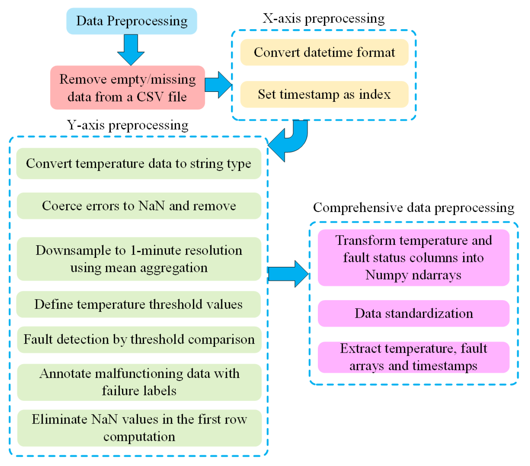
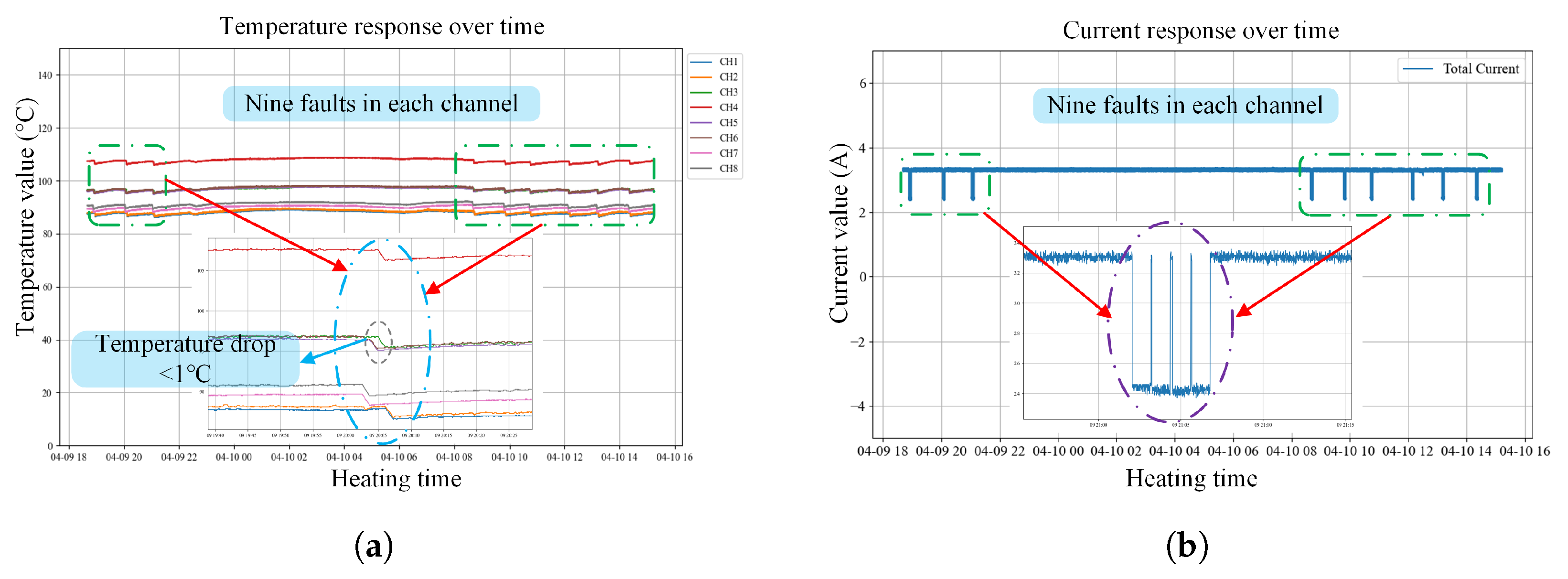
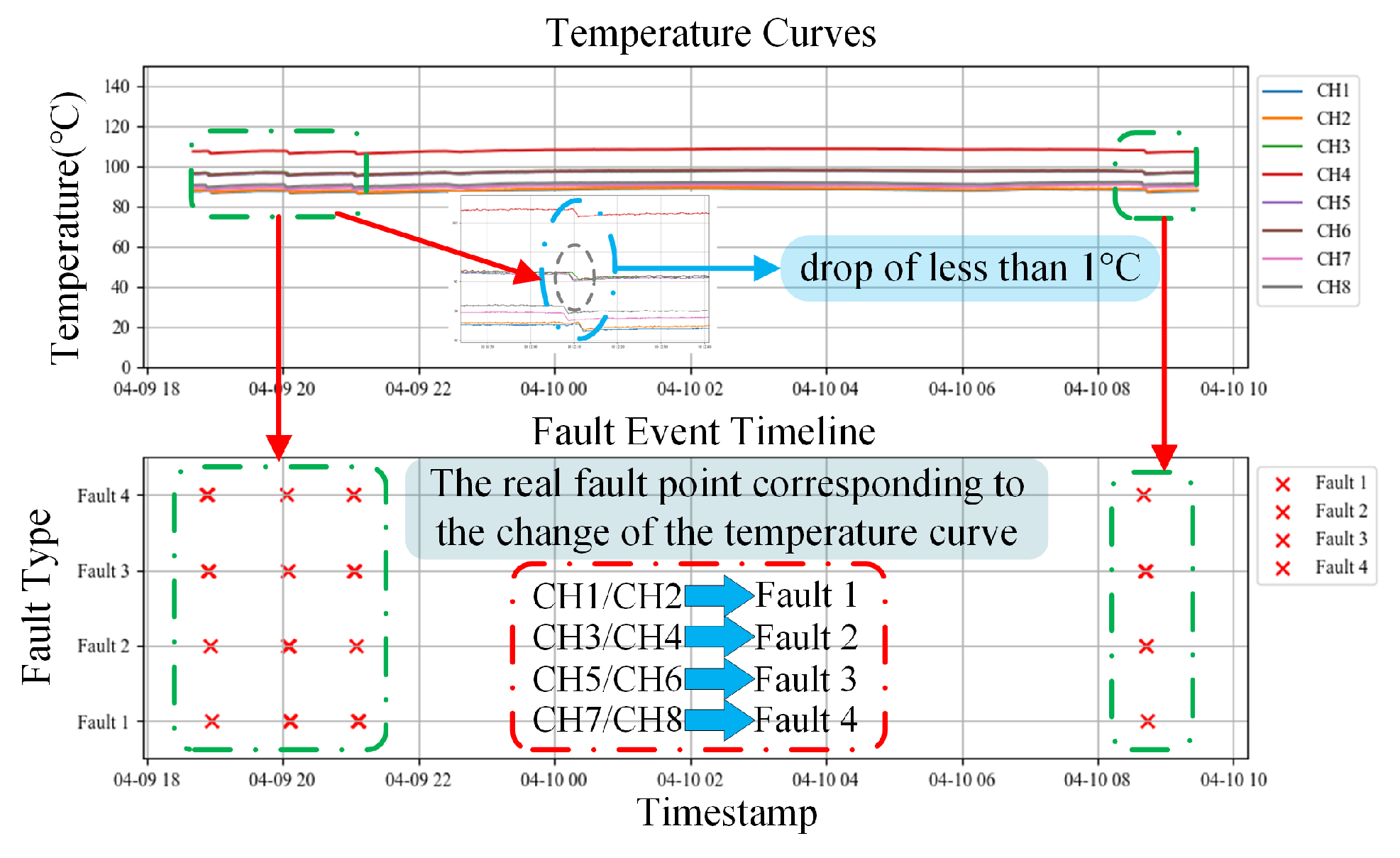
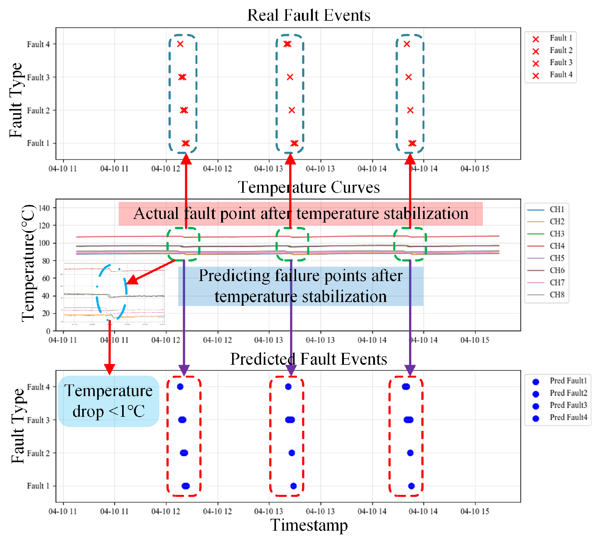
This study constructed a spatiotemporal fusion dataset using time-series temperature and current data obtained from the digital-twin platform. The initial step is to preprocess the entire dataset. Preprocessing transforms raw data into a format appropriate for model training, rectifies data-quality concerns, and enhances generalization, thereby improving model accuracy and reliability. Figure 8 illustrates the comprehensive preprocessing workflow. A dataset containing temperature and current measurements under standard operating conditions and during breakpoint failures is acquired for post-preprocessing.

4.2. Selection and Introduction of Fault Diagnosis Models

To assess the accuracy and stability of the selected model, this paper employs multiple loss functions. The losses considered are mean squared error (MSE), binary cross-entropy (BCE), and binary cross-entropy with logits (BCEWithLogits).

This study employs a 1D-CNN to preprocess data collected by a digital twin monitoring platform and subsequently performs fault diagnosis on the resampled data. To demonstrate the model’s effectiveness for fault diagnosis of the aluminum-block heating platform, the 1D-CNN is compared with two other classification algorithms. Using relevant evaluation metrics, the relative merits of the three models are assessed using relevant evaluation metrices. After preprocessing, the dataset is split chronologically into training, validation, and test sets to prevent temporal leakage. Specifically, the first 70% of the time-ordered samples is used for training, the next 10% is used for validation, and the final 20% is used for testing.

Table 2. Dataset partitioning.

Data Set Partitioning	Training	Validation	Test	Total
Data volume (number of samples)	888	99	247	1234
Normal samples (number of samples)	826	92	231	1149
Fault samples (number of samples)	62	7	16	85

reports the split statistics. The key implementation settings and hyperparameters for the three models, including the 1D-CNN, the BP neural network, and XGBoost, are summarized in

Table 3. Training hyperparameters and key implementation settings for the three fault-diagnosis models.

Item	1D-CNN	BP Neural Network	XGBoost
Train/validation/test split	7:1:2	7:1:2	7:1:2
Resampling	1 min (mean)	1 min (mean)	1 min (mean)
Fault labeling threshold (°C)	0.38	0.38	0.38
Input dimension	8	8	8
Dropout	0.2	0.2	–
Output vector size	4	4	4
Batch size	128	128	–
Epochs	100	100	–
Training method	Adam	Adam	Tree boosting
Learning rate	0.001	0.001	0.05
Loss	BCEWithLogitsLoss	BCEWithLogitsLoss	–
Number of trees	–	–	300
Max depth	–	–	5
Min child weight	–	–	1
Subsample	–	–	0.8
Colsample by tree	–	–	0.8
Gamma	–	–	0

.

The comparison indicates that one-dimensional convolutional neural networks are more computationally efficient, achieve lower loss values, and exhibit better responsiveness and stability.

Table 4. Accuracy under different loss functions.

Loss Function	1DCNN	BP Neural Network	XGBoost
MSE	95.14%	93.12%	89.47%
BCE	96.36%	93.52%	89.07%
BCEWithLogits	98.38%	95.14%	91.09%

reports the validation accuracy of each model trained with MSE, BCE, and BCEWithLogits.

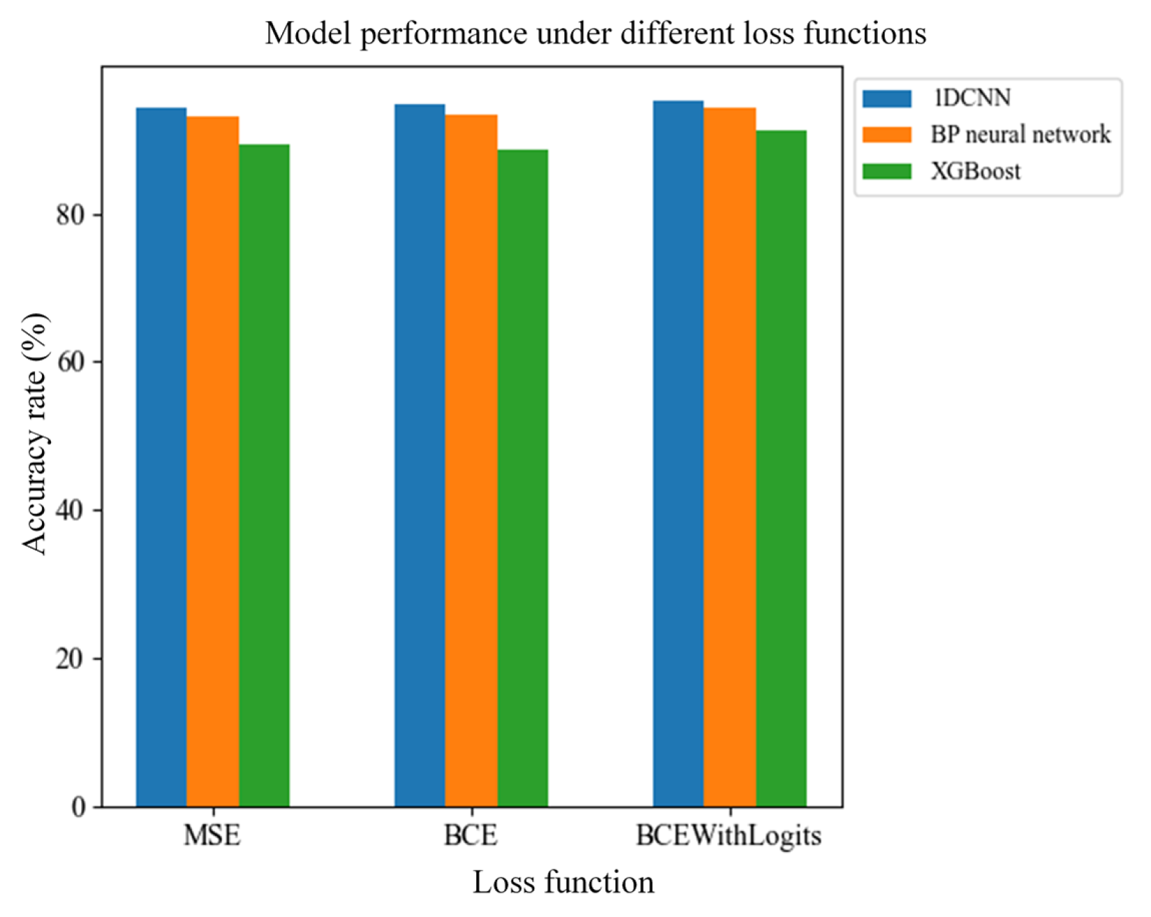
Figure 9 illustrates a comparison of the performance metrics of the three algorithms, derived from the data presented in Table 4. The plot highlights the strengths and weaknesses of each algorithm. Across the different loss functions, the 1D-CNN achieves, on average, an accuracy 2.7% higher than that of the traditional BP neural network and 6.75% higher than that of the XGBoost algorithm. The 1D-CNN architecture was selected for the temperature anomaly diagnosis task due to its exceptional performance in identifying temperature anomalies. In addition, the confusion matrix of the 1D-CNN is presented in

Table 5. Confusion matrix at the fault-versus-normal level on the test set.

	Predicted Normal	Predicted Fault
Actual Normal	TN = 230	FP = 1
Actual Fault	FN = 3	TP = 13

.

4.3. 1D-CNN Architecture and Training Configuration

After preprocessing, the raw measurement data are resampled at a 1 min interval using mean aggregation. Each sample is represented as an 8-dimensional temperature feature vector corresponding to the eight temperature channels. The input features are standardized via z-score normalization using the mean and standard deviation computed from the training set, and the same statistics are applied to normalize the test set.

The 1D-CNN reshapes the normalized 8-dimensional vector into a one-channel 1D sequence of length 8, enabling the convolutional layers to learn local correlations among the multi-channel temperature features. The network architecture is summarized in

Table 6. 1D-CNN architecture used for fault diagnosis.

Layer	Output Shape	Configuration
Input reshape	(1, 8)	8-D feature vector → 1 channel sequence of length 8
Conv1 + ReLU	(16, 6)	16 filters, kernel size 3, stride 1, padding 0
Conv2 + ReLU	(32, 4)	32 filters, kernel size 3, stride 1, padding 0
Flatten	(128)	32 × 4 → 128
Dropout	(128)	rate 0.2
FC1 + ReLU	(64)	128 → 64
FC2 (logits)	(4)	64 → 4

. No pooling or batch-normalization layers are used in this implementation. The hidden layers adopt ReLU activation functions, and a dropout layer with a rate of 0.2 is inserted before the fully connected classifier.

The network outputs a 4-dimensional logit vector corresponding to four fault-indicator labels. The normal condition is encoded as an all-zero indicator vector, whereas a fault condition is indicated when at least one indicator is positive. During inference, the logits are first mapped by a sigmoid function and then converted into binary indicators using a fixed threshold of 0.25. For evaluation, a sample is counted as correctly classified only when all four predicted indicators exactly match the ground-truth indicators.

For training, the Adam optimizer is employed with a learning rate of 0.001 and a weight decay of $1\times {10}^{-4}$. The loss function is BCEWithLogitsLoss. The batch size is set to 128, and the model is trained for up to 100 epochs. During training, the best checkpoint is selected based on validation performance and may be used for early stopping, while the test set is strictly held out for the final unbiased evaluation and reporting. The resulting fault-versus-normal performance of the 1D-CNN on the test set is summarized in

Table 7. Fault-versus-normal performance of the 1D-CNN on the test set.

Accuracy (%)	Precision (%)	Recall (%)	F1-Score (%)
98.38	92.86	81.25	86.67

, including accuracy, precision, recall, and F1-score.

5. Simulation and Experimental Results

5.1. Single-Channel System Identification Based on a Real Experimental Platform

To assess the efficacy of the proposed control method, a mathematical model of the controlled system was established on an actual experimental platform. System identification for a multi-point aluminum block heating temperature control system was conducted utilizing step-response experiments. Figure 10 illustrates an eight-channel platform wherein a TMS320F28335 (Texas Instruments, Dallas, TX, USA) regulates the temperature. Every channel is fitted with a low-voltage heater and a three-wire temperature sensor capable of measuring temperatures from −50 °C to 200 °C. The control architecture comprises a dual closed-loop configuration featuring an external temperature loop and an internal voltage loop. Real-time temperature data are obtained through the ModbusRTU protocol via an RS-485 interface and contrasted with the reference temperature to generate the error signal. Temperature regulation is achieved through a collaborative controller that integrates an enhanced backpropagation neural network with proportional-integral-derivative control. The controller generates a reference voltage that is contrasted with the measured voltage to modulate the input of the temperature-control system, consequently regulating the output temperature.

The temperature-control system is identified using the step-response method; the plant’s transfer function is given in Equation (31).

$$P\left(s\right)={\displaystyle \frac{26.5}{2150s+1}}{e}^{-10s}$$

(31)

The regulated system is represented and simulated within the MATLAB/Simulink (R2022b, MathWorks, Natick, MA, USA) framework. The plant model is identified from the physical platform in the simulations. A PID controller is employed to control the temperature. Figure 11 illustrates the system’s response when the temperature is maintained at 100 °C. The PID error signals e(k), e(k − 1), and e(k − 2) constitute the dataset, which is divided into a 75% training set, a 15% validation set, and a 10% test set. An enhanced BP neural network, trained using the Levenberg–Marquardt (LM) algorithm, is applied to the training set and subsequently validated on the validation set. Early stopping is implemented when the validation error remains unchanged for six successive iterations. Figure 12, Figure 13, Figure 14, Figure 15, Figure 16, Figure 17 and Figure 18 illustrates the training mean squared error (MSE), training status, error histogram, and regression results for each dataset.

The training results indicate that a standalone PID controller achieves temperature stabilization at approximately 2000 s. During training, the mean squared error (MSE) attained a minimum of 0.5 at iteration 500; the gradient norm displayed a consistent decline; the damping factor ultimately stabilized at 1; and the error histogram approximated a normal distribution. The accuracies for the training, validation, and test sets all surpassed 99%, demonstrating excellent training performance.

The trained LM-BP neural-network is incorporated with the PID controller and compared with standalone PID control and PID combined with a conventional BP neural network. The simulation comprises two phases. During Stage 1 (heat-up), the temperature is elevated from 0 °C to 100 °C and permitted to stabilize, after which control transitions from the PID controller to the neural-network controller. During Stage 2 (setpoint tracking), the temperature oscillates between 100 °C and 105 °C, returning to 100 °C, and this sequence is repeated for several cycles to assess both step-up and step-down performance. Figure 19 illustrates the comprehensive time response of the control system. Figure 20a depicts the time response for the initial positive step, and the time response for the final positive step is presented in Figure 20b.

Compared with standalone PID control and PID+BP control, the PID+LM-BP cooperative controller achieves superior performance, as shown in Figure 19. The response times under PID and PID+BP control are approximately 2000 s and 1500 s, respectively, whereas the PID+LM-BP cooperative controller reaches a stable state within about 200 s, corresponding to response-speed improvements of nearly 90% and 86%, respectively. Figure 20a demonstrates that during the initial positive step, when the neural network has just started learning, the control performance is poor; however, by the final positive step, the neural network achieves good control performance, as shown in Figure 20b. The outputs of the PID and neural network during the control process, as well as the combined control signal PID + neural network, are plotted in Figure 21a and Figure 21b, respectively.

As shown in Figure 21, the final control command is formed by directly adding the outputs of the PID controller and the neural-network controller, without introducing any explicit hard switching logic. In the initial phase, the PID output provides a robust baseline regulation, while the neural-network output is progressively refined via online Levenberg–Marquardt updating. As learning converges and the tracking error decreases, the required PID correction correspondingly becomes smaller. The PID contribution is regarded as effectively negligible when the magnitude of the PID output remains below 5% of the combined control command for a sustained period, indicating that the neural-network term has become dominant.

5.2. Temperature Control Test Results from the Aluminum-Block Heating Digital Twin Platform

This study described a digital twin monitoring system for the aluminum-block heating platform that utilizes a Windows desktop application for visualization. The application features a real-time clock display, facilitates communication between the heating platform and the monitoring system, and manages data acquisition, processing, and visualization. Experiments were performed utilizing an LM-optimized BP neural-network control method, with parameter values consistent with those employed in the simulation. The experimental configuration was identical to that depicted in Figure 10. The experimental parameters were as follows: a sampling interval of 0.1 s; a controller sampling resolution of 12 bits; a sensor resolution of 0.1 °C; and a maintained ambient temperature of 30 °C. The CH1 temperature was adjusted to reach 100 °C; once stabilized, feedforward control was implemented to elevate the temperature from 100 °C to 105 °C. Figure 22 illustrates the time response and the impact of feedforward control on the aluminum-block heating system.

Figure 22 illustrates that the overshoots of the controlled system under PID control, PID+BP control, and PID+LM-BP control are 9 °C, 5 °C, and 3 °C, respectively, and the settling times for positive-step regulation are 20 min, 8 min, and 6 min, respectively. The optimization technique presented in this study achieves a faster response and smaller overshoot than both standalone PID control and PID combined with a conventional BP neural network. Consequently, the proposed PID+LM-BP cooperative control strategy significantly enhances the overall control performance of the system. Both simulations and experiments validate the effectiveness of the proposed method.

5.3. Fault Diagnosis Based on an Aluminum-Block Heating Virtual Platform

Simulated fault diagnosis experiments were performed on the aluminum block heating platform. A digital-twin-inspired monitoring system was employed to present temperature measurements and related data on the monitoring interface in real time. The temperatures of the eight channels and the bus current were displayed through the respective controls, and their historical trends were illustrated in tables. Upon collection, the temperature and current data were preserved in a CSV file for future fault diagnosis.

During the collection of temperature data, DSP was employed to disconnect the heaters, while a button was utilized to control the relay for activating and deactivating the heaters. At each instance, two heaters were deactivated and maintained offline for one minute before the resumption of heating. The temperature profiles were captured through real-time data acquisition by the digital twin monitoring system. Figure 23a,b illustrate the temperature and current waveforms when the input control voltage was set to 20 V and each heater was disconnected once. Figure 23 illustrates that temperature and current anomalies transpired between 14:15 and 14:25, with each power interruption enduring approximately 1 min. During the disconnections, the temperature gradually decreased, averaging a decline of less than 1 °C. The total current decreased four times consecutively, plummeting from 4.5 A to 3.3 A, signifying a substantial alteration in current. Each incident signifies that the heaters of two contiguous channels of the aluminum-block heating platform were disengaged, with each channel encountering one such fault.

The temperature versus time waveform was recorded with the input voltage set at 15 V. In the temperature-increase phase, the DSP instructed the relay to disconnect each heater once, and after the temperature stabilized, it commanded two further disconnections. Figure 24a,b illustrate the temperature and current waveforms under these conditions, respectively. As illustrated in Figure 24a, each channel encountered a singular fault during the temperature increase. As the temperature reached close to equilibrium, each channel experienced a fault, with channels 3 and 4 displaying an additional fault. Once the temperature reached full stabilization, each channel encountered an additional fault, with the average temperature decline during each incident being under 1 °C. As illustrated in Figure 24b, the current diminished in four consecutive stages during the temperature-increase phase. As the temperature approached equilibrium, the current diminished in five consecutive stages. Once the temperature was fully stabilized, the current diminished in an additional four increments. In each instance, the current decreased from approximately 3.4 A to roughly 2.6 A.

After elevating the aluminum block to a stable temperature with a constant input voltage of 15 V, the DSP was employed to collect the initial dataset by intermittently disconnecting the heater. The initial dataset underwent preprocessing: each channel pair was assigned a fault label, and a threshold was established. Specifically, the temperature signals were resampled at a 1 min interval using the mean value, and a sample was labeled as a fault when the absolute minute-to-minute change of the one-minute mean temperature exceeded the threshold. Following the chronological split of the dataset into a 7:1:2 ratio (training: validation: test), a 1D-CNN was employed to identify and pinpoint anomalies in the temperature data. Figure 25a,b illustrate the temperature and current profiles for the wire-break fault test performed after temperature stabilization. By breaking nine wires, a deliberate induction was applied to each channel’s heater to acquire adequate fault labels.

Figure 26 illustrates the temperature image of the training set post-data preprocessing, with the actual fault points indicated by red ‘x’ symbols. Figure 27 illustrates the temperature images of the test set, depicting actual and predicted fault points before and after the 1D-CNN prediction. Predicted fault points are denoted by blue ’‘o’ symbols, whereas actual fault points are indicated by red ‘x’ symbols. Figure 27 indicates that following the 1D-CNN prediction, all faults are identified and localized at their respective times of occurrence, with the predicted and actual fault points closely aligning at 12:00, 13:00, and 14:00.

6. Conclusions

This study proposed a dual AI-driven approach for temperature regulation and fault diagnosis of an aluminum block heating platform, utilizing digital-twin-inspired monitoring systems. The method attains accurate regulation of a multi-point aluminum-block heating system by integrating a backpropagation neural network, augmented with a LM-optimized BP algorithm, with traditional PID control. The method enhances the system’s response speed and stability in temperature regulation, while also facilitating real-time, precise fault detection and localization through a 1D-CNN model during fault occurrences. The dual-AI system autonomously refines the composite control command by progressively learning the neural-network compensation term via online Levenberg–Marquardt updating, and it enables rapid fault detection. The digital-twin-inspired monitoring system facilitates real-time surveillance and proactive alerts through the aggregation of high-precision data. The experimental and simulation findings indicate that the proposed method improves the precision of temperature control and the efficiency of fault diagnosis for aluminum block heating platforms, exhibiting significant potential for engineering applications. The incorporation of dual AI markedly improves the system’s intelligence and robustness, facilitating intelligent and highly reliable operation of industrial heat treatment systems.