Flexible Day-Ahead Scheduling of a Cascade Hydro-Wind-Solar-Thermal-Storage System Including Hybrid Pumped Storage

Abstract

To advance the modernization of power systems, the role of hydropower has transitioned from mere energy generation to serving as both a primary energy provider and a critical flexibility resource. However, conventional day-ahead scheduling methodologies for cascaded hydropower often prove inadequate in mitigating the short-term power imbalances induced by renewable energy variability, primarily due to an oversimplification of operational constraints. To fully harness the regulatory potential of hydropower, this paper proposes an optimal day-ahead scheduling strategy for a cascade hydro-wind-solar-thermal-storage system incorporating hybrid pumped storage (HPS). First, leveraging the operational characteristics of HPS, this study evaluates its capacity for renewable energy accommodation and identifies key challenges in power balancing from the perspectives of water resource management and energy dispatch. Second, a collaborative optimization framework is established. By introducing the concept of an “allowable reservoir water level fluctuation range” within the day-ahead dispatch cycle, the framework constrains the deviation between the actual end-of-period water level and its predefined target, thereby ensuring strict adherence to medium-to-long-term operational boundaries. Finally, case studies conducted on a modified IEEE 33-node system demonstrate that the integration of HPS significantly enhances system regulation capabilities. The results confirm that the proposed strategy contributes to secure, economical, and low-carbon grid operation while maintaining reservoir sustainability.

1. Introduction

Aligned with China’s national commitments to carbon peaking and carbon neutrality, the national energy strategy is driving a structural transformation of the power sector [1,2,3,4]. Large-scale integration of variable renewable energy (VRE) has exacerbated system flexibility shortages, posing growing challenges to grid stability under widening supply–demand imbalances [5,6,7,8]. In response, Chinese academia and industry have put forward the concept of hydropower function reconfiguration [9], which repositions conventional hydropower from a pure energy supplier to a dual-role resource providing both stable power generation and flexible regulation. This shift has made hydropower an indispensable supporting resource for power systems with high VRE penetration. To fully tap this regulatory potential, two practical pathways have been identified. First, moving beyond traditional short-term scheduling practices focused solely on peak shaving and developing optimization frameworks tailored to routine dispatch cycles. Second, enhancing regulation capacity via physical retrofits, such as installing reversible turbine units or auxiliary pumping facilities at conventional cascade hydropower stations to establish hybrid pumped storage (HPS) systems [10].

To date, extensive research has focused on optimizing cascade hydropower operations within the day-ahead dispatch framework. Early studies optimized day-ahead peak-shaving schedules for cascade configurations via customized objective functions [11,12]. The effectiveness of hydro-solar complementarity for day-ahead peak regulation was verified in [13], while ref. [14] proposed a coordinated operation strategy for cascade hydro-wind systems that accounts for system uncertainties. Later work refined day-ahead dispatch schemes using source-load matching metrics [15], and improved the commitment accuracy of thermal units by integrating demand response and pumped storage resources [16]. More recent studies introduced data-driven robust optimization methods for cascade hydro-solar-storage systems to mitigate renewable output fluctuations within the day-ahead cycle [17]. In parallel, retrofitting conventional cascade hydropower stations into HPS systems has emerged as a promising approach to boost scheduling flexibility [18-19]. Representative explorations include complementary scheduling rules for HPS-PV systems under the day-ahead framework [20], short-term peak-shaving patterns for operational HPS stations tailored to day-ahead dispatch [21], and dynamic reservoir capacity control strategies for multi-stage HPS stations aligned with day-ahead operational requirements [22]. However, most existing studies on HPS scheduling remain confined to the day-ahead scale; for example, prior work on retrofitted HPS plants did not adequately account for the stochastic variability of renewable generation, nor did it address the inherent coupling between power dispatch and water management in cascade systems [23].

Collectively, existing research reveals persistent limitations in current day-ahead scheduling frameworks for cascade hydropower systems. Most studies prioritize optimizing unit commitment and generation output to improve VRE accommodation, but often overlook the inherent operational constraints of hydropower units—such as non-dispatchable intervals caused by mandatory unit vibration zones—that restrict the ability to track day-ahead dispatch signals. This gap leaves conventional frameworks unable to handle output fluctuations of VRE within the 24-h dispatch window, limiting hydropower’s contribution to system flexibility. Compared with standalone pumped storage plants, cascade hydropower systems face unique unresolved challenges in both energy and water management under the day-ahead dispatch framework. On the energy side, vibration zone constraints fragment the feasible operating range of hydropower units, making it difficult to follow scheduled power trajectories. On the water side, conventional day-ahead scheduling methods that enforce strict equality between end-of-period reservoir levels and predefined targets are poorly suited to cascade systems. Unlike isolated pumped storage reservoirs, which are largely unaffected by natural inflows, cascade and HPS systems must account for variable natural runoff while complying with medium-to-long-term scheduling boundaries that restrict short-term operational flexibility. Rigid end-of-period level constraints often render day-ahead optimization models infeasible or unnecessarily curtail dispatch flexibility.

While various flexible scheduling approaches have been proposed to mitigate the limitations of rigid end-of-period constraints, they differ significantly in their treatment of reservoir water levels. Flexible terminal reservoir-level methods allow the end-of-period water level to vary within a certain range, but they often lack a direct mechanism to ensure compliance with medium-to-long-term operational targets. Operating-band methods define allowable upper and lower bounds for reservoir levels throughout the entire scheduling horizon, yet they may not specifically address the deviation between the actual and target end-of-period levels. Soft endpoint-constraint methods replace strict equality constraints with penalty terms in the objective function, which can lead to excessive violations if the penalty weights are not carefully tuned. In contrast, the proposed allowable reservoir water-level fluctuation range introduces a targeted relaxation that explicitly constrains the deviation between the actual end-of-period water level and its predefined target. This approach strikes a balance between short-term dispatch flexibility and long-term water resource management requirements, ensuring that the day-ahead schedule remains feasible while strictly adhering to medium-to-long-term operational boundaries.

Beyond the temporal coordination between medium-to-long-term water resource management and day-ahead dispatch, modern power systems require operational flexibility to be provided across multiple dimensions, including ancillary service markets and regulatory frameworks. In practice, grid operators impose explicit ramp-rate limits, primary and secondary frequency response mandates, and operating codes that govern how conventional and pumped-storage hydropower participate in real-time balancing and day-ahead reserve procurement [24,25]. For instance, regional grid operating codes often stipulate that hydropower units must maintain a minimum proportion of system spinning reserves to counteract renewable forecast errors, while thermal units are subject to ramping constraints aligned with automatic generation control (AGC) requirements [26]. Despite these complex, multi-layered regulatory policies, existing day-ahead scheduling studies for cascade hydropower frequently oversimplify operational regulation capabilities, implicitly treating them as binary classifications—either seasonal (long-term) or daily (short-term). This simplification fails to reflect the nuanced reality of ancillary service markets, where flexibility products such as ramp-rate reserves and frequency response are procured and compensated independently. To bridge this gap, the proposed day-ahead scheduling framework explicitly embeds real-world regulatory constraints and market rules into its optimization model. The ramp-rate limits, spinning reserve requirements, and vibration zone restrictions are not merely technical assumptions but are directly derived from contemporary grid operating codes and ancillary service market clearing mechanisms. By doing so, the model transcends a simplistic seasonal-daily dichotomy and provides a realistic representation of how policy constraints shape the dispatch of cascade hydro-wind-solar-thermal-storage systems.

While prior work addresses hydro-wind-PV coordination, pumped-storage operation, and flexible scheduling in isolation, this study integrates these elements within a single cascade hydro-wind-solar-thermal-storage framework under an allowable end-of-period water-level fluctuation range. To address these gaps, this paper develops an optimal day-ahead scheduling strategy for cascade hydro-wind-solar-thermal-storage systems incorporating HPS, which can be readily extended to conventional cascade hydropower systems. A core innovation of this work is the introduction of an allowable water level fluctuation range for reservoir endpoints, which relaxes rigid end-of-period-level constraints to enhance day-ahead dispatch feasibility while ensuring compliance with long-term water resource management requirements. The proposed framework coordinates heterogeneous resources—including conventional cascade hydropower, HPS units, VRE, thermal power units, and distributed energy storage—to balance three key objectives: maximizing VRE accommodation, maintaining grid operational stability, and adhering to long-term reservoir operation rules.

2. Optimal Scheduling Capability and Challenges of Hybrid Pumped Storage in Renewable Energy Consumption

2.1. Assessment of Renewable Energy Consumption Ability for Hybrid Pumped Storage

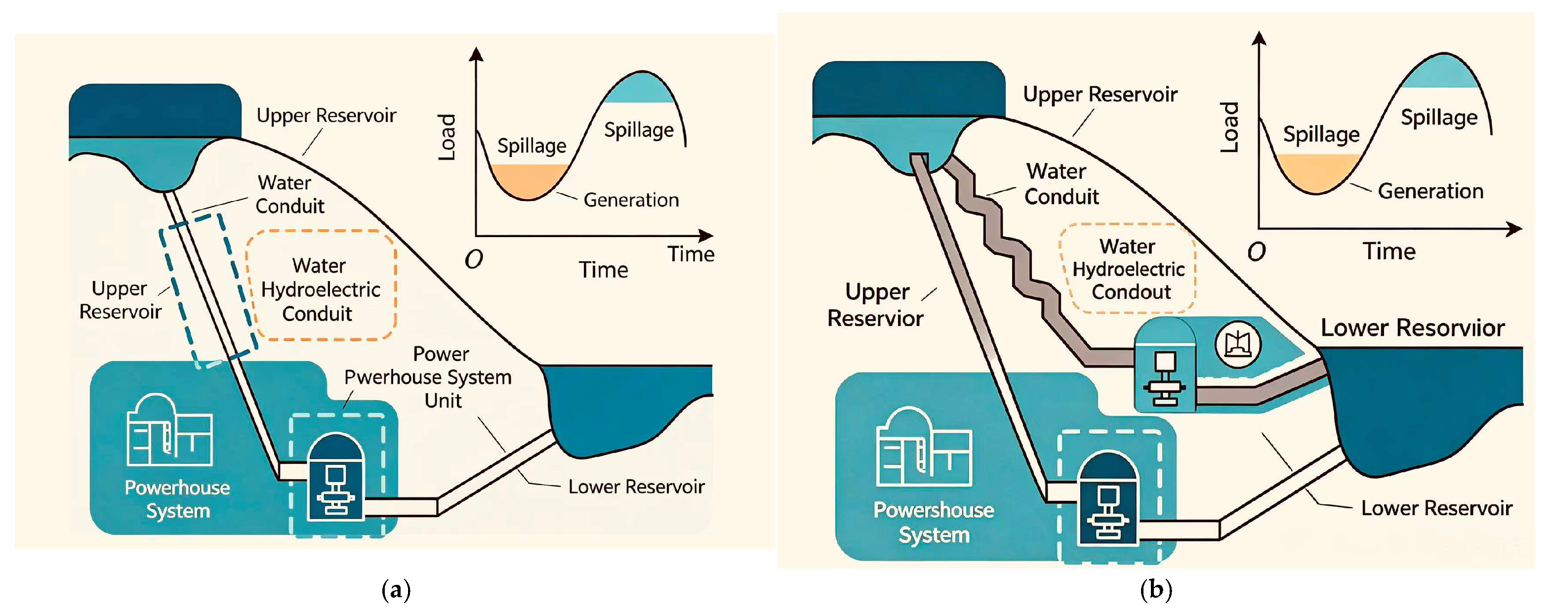
In the day-ahead stage, wind power exhibits pronounced anti-peak-shaving characteristics, leading to substantial curtailment during off-peak hours. While conventional cascade hydropower mitigates this issue primarily by optimizing unit commitment and output, its capacity to absorb wind power during these low-demand periods remains limited, as illustrated in Figure 1a.

Conversely, hybrid pumped storage (HPS) integrates the energy time-shift feature of conventional storage. This shifts the operational paradigm from mere “peak shaving” to an integrated “peak shaving and valley filling” mode, significantly bolstering regulation capability during off-peak hours, as shown in Figure 1b. At intra-day timescales, the stochastic volatility of wind power generates new balancing requirements. Unlike conventional turbines constrained by ramp rates, HPS leverages the rapid responsiveness of reversible units to compensate for these fluctuations, thereby achieving superior mitigation of short-term renewable intermittency.

2.2. Assessment of Hybrid Pumped Storage in Enabling Real-Time Grid Balancing

From the perspective of energy dispatch, unlike the continuous operation of thermal units, the feasible operating zones of hydro and pumped storage units are fragmented into discrete intervals due to forbidden vibration zones [11]. This discontinuity precludes precise tracking of real-time power dispatch signals. For instance, even if ramping capabilities allow, a regulation command requiring an output within the vibration zone (P₁, P₂) forces the unit to settle at the boundary values (P₁ or P₂). Such inherent physical limitations hinder the system’s ability to meet upward or downward regulation demands, potentially leading to load shedding or renewable curtailment during severe mismatches.

Regarding water management, short-term scheduling of cascade systems must adhere to medium-to-long-term reservoir level trajectories. While day-ahead scheduling typically enforces a strict equality constraint (end-level equals target level), this approach is ill-suited for intra-day rolling dispatch. In shorter time horizons, the stochastic nature of operations makes precise endpoint control infeasible. Imposing a rigid terminal level constraint often leads to model infeasibility or unnecessarily curtails operational flexibility in the final hour. Therefore, a novel methodology is imperative to constrain the water level deviation at the end of the dispatch period rather than enforcing an exact match.

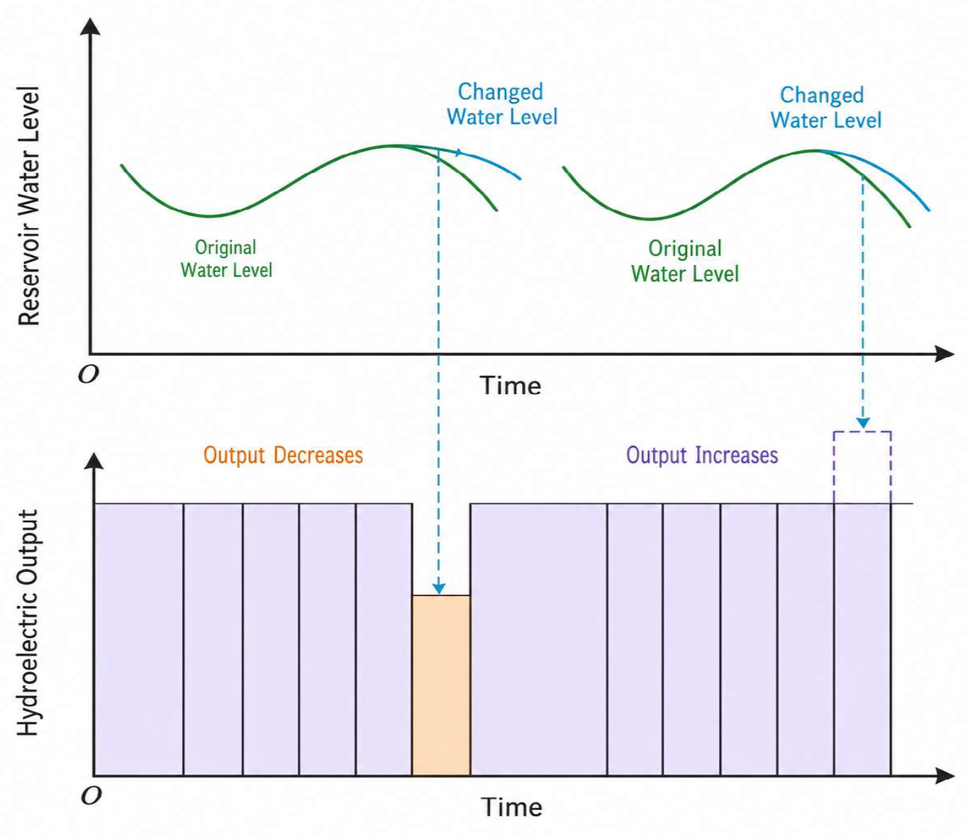
Furthermore, hydro-electrical coupling is intrinsically tight within hybrid pumped storage systems, where electrical fluctuations directly induce hydraulic variations. As illustrated in Figure 2, a reduction in real-time unit output triggers a rise in reservoir levels, whereas an increase in generation leads to a drawdown. Consequently, the frequent power adjustments necessary for real-time grid balancing cause uncontrolled reservoir level oscillations, complicating the tracking of target end-of-period levels. Conversely, imposing strict limits on intra-hour water level deviations can curtail generation flexibility. Thus, a reciprocal interaction exists: real-time dispatch decisions influence reservoir dynamics, and these hydraulic constraints, in turn, feedback to restrict generation capabilities.

3. Model Formulation for Optimal Scheduling for the Cascade Hydro-Wind-Solar-Thermal-Storage Hybrid System

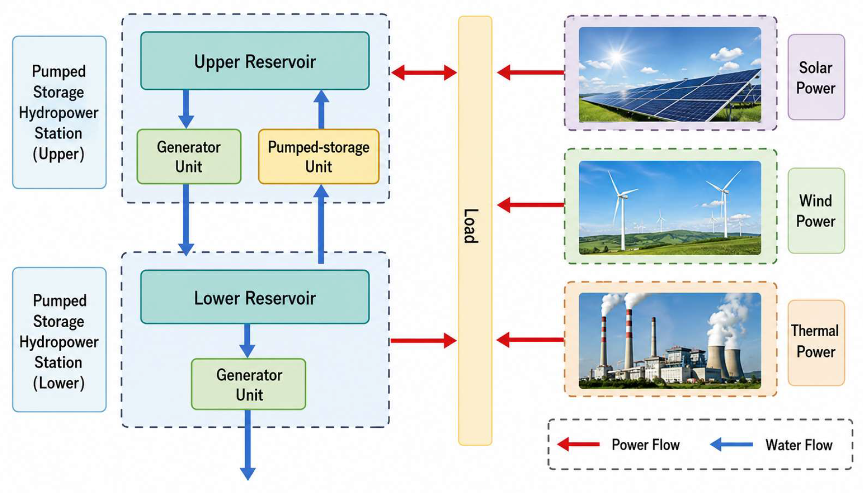
As illustrated in Figure 3, the proposed architectural framework integrates a hybrid pumped storage (HPS) facility into a conventional cascade hydropower system. This is achieved by retrofitting one cascade station with reversible turbine units, thereby enabling coordinated dispatch across thermal, wind, and solar generation assets.

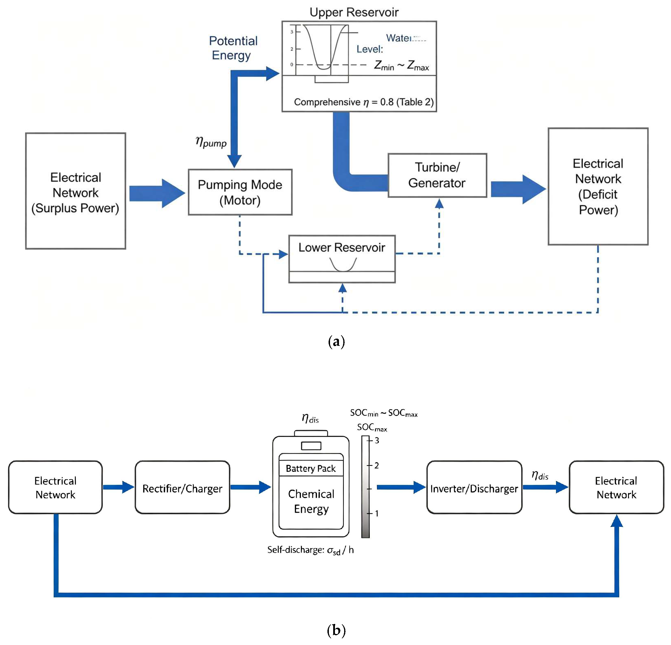
Figure 4. Schematic diagram of energy flows for (a) hybrid pumped storage (HPS) and (b) electrochemical energy storage (ESS). The diagram explicitly illustrates the energy conversion pathways, round-trip efficiencies (η), state-of-charge (SOC) boundaries, and self-discharge mechanisms.

3.1. Objective Function

The objective function for day-ahead scheduling is formulated as Equation (1). Regarding the daily depreciation cost of the pumped storage units, while it typically encompasses both unit installation and reservoir construction expenses, this study focuses on a retrofit context. Since the system leverages existing reservoirs within the conventional cascade, the reservoir capital costs are exempted from the calculation.

minf₁ = (C_g + C_k + C_q + C_T + C_b + C_h + C_p + C_s)

(1)

(1)

Fuel cost of thermal power units

$$C_{\mathrm{g}}={\displaystyle \sum _{t=1}^{24}}{\displaystyle \sum _{i=1}^N}{U}_{i,t}(a_i{P}_{\mathrm{G},i,t}^2+b_i{P}_{\mathrm{G},i,t}+c_i)$$

(2)

The quadratic function $a_i{P}_{\mathrm{G},i,t}^2+b_i{P}_{\mathrm{G},i,t}+c_i$ represents the thermal efficiency (heat rate) curve of thermal unit i. The coefficients a_i, b_i, c_i are derived from the unit’s physical characteristics and are expressed in USD/MW², USD/MW, and USD, respectively. Specific values for these parameters are provided in Table 1.

Table 1. Technical parameters of thermal power units.

Unit No.	Pmin (MW)	Pmax (MW)	${\mathit{R}}_{\mathbf{G}}^{\mathbf{U}}$	${\mathit{R}}_{\mathbf{G}}^{\mathbf{D}}$	${\mathit{T}}_{\mathit{i}}^{\mathbf{ON}}$	${\mathit{T}}_{\mathit{i}}^{\mathbf{OFF}}$	Start-Up Cost (USD/start)	ai	bi	ci
1	30	100	2.0	2.0	4	3	120	0.0015	0.025	8.0
2	20	60	1.5	1.5	3	2	80	0.0020	0.030	5.0
3	15	40	1.0	1.0	2	1	50	0.0025	0.035	3.0

Table 1. Technical parameters of thermal power units.

Unit No.	Pmin (MW)	Pmax (MW)	${\mathit{R}}_{\mathbf{G}}^{\mathbf{U}}$	${\mathit{R}}_{\mathbf{G}}^{\mathbf{D}}$	${\mathit{T}}_{\mathit{i}}^{\mathbf{ON}}$	${\mathit{T}}_{\mathit{i}}^{\mathbf{OFF}}$	Start-Up Cost (USD/start)	ai	bi	ci
1	30	100	2.0	2.0	4	3	120	0.0015	0.025	8.0
2	20	60	1.5	1.5	3	2	80	0.0020	0.030	5.0
3	15	40	1.0	1.0	2	1	50	0.0025	0.035	3.0

Where N is the number of thermal power units; U_i,t is the commitment status of unit at time interval (1 for on, 0 for off); a_i, b_i, c_i are the quadratic fuel cost coefficients of unit; P_G,i,t is the active power output of unit at time interval.

(2)

Start-up and shut-down costs of thermal power units

$$C_{\mathrm{k}}={\displaystyle \sum _{t=1}^{24}{\displaystyle \sum _{i=1}^N(U_{i,t}(}}1-U_{i,t-1})+U_{i,t-1}(1-U_{i,t}))C_i$$

(3)

where C_i is start-up and shut-down cost of the thermal unit. In the context of day-ahead scheduling with a 1-h time resolution, the physical time differences between warm and cold starts are primarily captured through the minimum up/down-time constraints ($T_i^{\mathrm{ON}}$ and $T_i^{\mathrm{OFF}}$). The start-up cost C_i in Equation (3) represents a comprehensive cost that accounts for both warm and cold start conditions, which is a standard modeling practice in hour-level unit commitment problems. The specific value of C_i is listed in Table 1.

(3)

Renewable energy imbalance penalty cost

$$C_{\mathrm{q}}=a_{\mathrm{L}}{\displaystyle \sum _{t=1}^{24}(\Delta P_{\mathrm{W},t}+\Delta P_{\mathrm{pv},t})}$$

(4)

where a_L is the penalty coefficient for renewable energy imbalance; ΔP_W,t and ΔP_pv,t are the curtailed wind power and curtailed solar power at time interval, respectively.

(4)

Carbon emission cost

$$C_{\mathrm{T}}={\delta }_{\mathrm{T}}(m_{{\displaystyle \sum }}-m_{\mathrm{B}}-m_{\mathrm{D}})+({\delta }_{\mathrm{Y}}+{\delta }_{\mathrm{C}})m_{\mathrm{B}}$$

(5)

where δ_T is the unit price of carbon trading; δ_Y is the unit cost of CO₂ transport; δ_C is the unit cost of CO₂ storage; mΣ is the total daily carbon production of the system; m_B is the total daily carbon capture amount of the system; m_D is the total daily carbon emission allowance of the system.

(5)

Variable operation and maintenance (O&M) cost for all non-thermal generation units, including conventional hydro, wind, and solar power

$$C_{\mathrm{h}}={\displaystyle {\displaystyle \sum _{i=1}^I}{\displaystyle \sum _{t=1}^T{\displaystyle \sum _{j=1}^J[U_{i,j,t}^{\mathrm{trad}}(1-U_{i,j,t-1}^{\mathrm{trad}})S_{i,j}^{\mathrm{on}}+U_{i,j,t-1}^{\mathrm{trad}}(1-U_{i,j,t}^{\mathrm{trad}})S_{i,j}^{\mathrm{off}}]}}}+k_{\mathrm{trad}}{\displaystyle {\displaystyle \sum _{i=1}^I}{\displaystyle \sum _{t=1}^T{\displaystyle \sum _{j=1}^J{P}_{i,j,t}^{\mathrm{trad}}}}}$$

(6)

where T, I, J, and S denote the scheduling horizon, the number of cascaded hydropower stations, the number of hydropower units, and the number of pumped-storage units, respectively; $P_{i,j,t}^{\mathrm{trad}}$ and $U_{i,j,t}^{\mathrm{trad}}$ represent the power output and the on/off status variable of generation units (subscript j covers hydro, wind, solar, etc.) at level i and time t, respectively; $S_{i,j}^{\mathrm{on}}$ and $S_{i,j}^{\mathrm{off}}$ are the start-up and shut-down costs of hydropower units, respectively; k_trad is the unified variable O&M cost coefficient (USD/MWh) applied to all non-thermal assets in the system.

(6)

Operation and maintenance cost of pumped-storage units

$$\begin{array}{l}{C}_{\mathrm{p}}={\displaystyle \sum _{i=1}^I{\displaystyle \sum _{t=1}^T{\displaystyle \sum _{s=1}^S\left\{k_{\mathrm{gen}}{P}_{i,s,t}^{\mathrm{gen}}+k_{\mathrm{pump}}{P}_{i,s,t}^{\mathrm{pump}}\right.}}}+C_s^{\mathrm{gen}}[(1-U_{i,s,t-1}^{\mathrm{gen}})U_{i,s,t}^{\mathrm{gen}}+(1-U_{i,s,t-1}^{\mathrm{pump}})U_{i,s,t}^{\mathrm{pump}}]+\\ C_s^{\mathrm{pump}}[(1-U_{i,s,t}^{\mathrm{gen}})U_{i,s,t-1}^{\mathrm{gen}}+(1-U_{i,s,t}^{\mathrm{pump}})U_{i,s,t-1}^{\mathrm{pump}}]\}\end{array}$$

(7)

where k_gen and k_pump are the generation cost coefficient and pumping cost coefficient of pumped-storage units, respectively. $P_{i,s,t}^{\mathrm{gen}}$ and $P_{i,s,t}^{\mathrm{pump}}$ are the power generation output and the pumping power input of pumped-storage unit at bus and time, respectively; $C_s^{\mathrm{gen}}$ and $C_s^{\mathrm{pump}}$ are the start-up cost and shut-down cost of pumped-storage unit s, respectively; $U_{i,s,t}^{\mathrm{gen}}$ and $U_{i,s,t}^{\mathrm{pump}}$ are the operation status variables of pumped-storage unit at bus and time under power generation and pumping modes, respectively;

(7)

Daily depreciation cost of pumped-storage units

$$C_{\mathrm{s}}={\gamma }_{\mathrm{s}}{P}_{\mathrm{all}}^{\mathrm{ps}}{\displaystyle \frac{{(1+r)}^{N}r}{365[{\left(1+r\right)}^N-1]}}$$

(8)

where γ_s represents the unit installed capacity construction cost of the pumped-storage unit, with a value of 528.6 USD/kW; $P_{\mathrm{all}}^{\mathrm{ps}}$ is the total installed construction capacity of the pumped-storage unit; r is the discount rate; N is the depreciation period of the pumped-storage unit.

(8)

Fixed O&M cost for thermal units

$$C_{\mathrm{b}}={\displaystyle \sum _{t=1}^{24}{\displaystyle \sum _{i=1}^N{K}_i}}{U}_{i,t}$$

(9)

where K_i is the fixed O&M cost rate (USD/h) for thermal unit, and U_i,t is its commitment status.

3.2. Constraints

(1)

Operation constraints of thermal units

Within each dispatch interval, the power output, ramping capability, and the duration of operation and shutdown for thermal units must be maintained within specific limits.

$$\left\{\begin{array}{l}{u}_{i,t}{P}_{\mathrm{G}}^{\mathrm{MIN}}⩽P_{\mathrm{G},i,t}⩽u_{i,t}{P}_{\mathrm{G}}^{\mathrm{MAX}}\hfill \\ P_{\mathrm{G},i,t+1}-P_{\mathrm{G},i,t}⩽R_{\mathrm{G}}^{\mathrm{U}}\Delta t\hfill \\ P_{\mathrm{G},i,t}-P_{\mathrm{G},i,t+1}⩽R_{\mathrm{G}}^{\mathrm{D}}\Delta t\hfill \\ T_i^{\mathrm{ON}}⩾T_{\mathrm{ON}}^{\mathrm{MIN}}\hfill \\ T_i^{\mathrm{OFF}}⩾T_{\mathrm{OFF}}^{\mathrm{MIN}}\hfill \end{array}\right.$$

(10)

Regulatory context of ramping constraints: The upward and downward ramping limits ($R_{\mathrm{G}}^{\mathrm{U}}$ and $R_{\mathrm{G}}^{\mathrm{D}}$) in Equation (9) are established in accordance with the primary frequency response mandates and automatic generation control (AGC) requirements stipulated in regional grid operating codes [27]. These constraints ensure that thermal units can provide ancillary services such as ramp-rate reserves, which are procured through day-ahead ancillary service markets to accommodate the stochastic variability of renewable generation. The numerical values of the ramp-rate limits and of the minimum up/down times used in the case study are unit-specific data taken from the technical documentation of the studied thermal units and are listed in Table 1; the obligation to represent and observe such limits follows from the operating code cited as [27], not from the numerical values reported in [24,25,26].

Where $P_{\mathrm{G}}^{\mathrm{MIN}}$ and $P_{\mathrm{G}}^{\mathrm{MAX}}$ are the minimum stable generation level and rated capacity of thermal units, respectively, in MW; $R_{\mathrm{G}}^{\mathrm{U}}$ and $R_{\mathrm{G}}^{\mathrm{D}}$ are the ramp-up and ramp-down rate limits of thermal units, respectively, in MW/min; $T_i^{\mathrm{ON}}$ and $T_i^{\mathrm{OFF}}$ are the continuous operation time and continuous shutdown time of thermal unit, respectively, in hours; $T_{\mathrm{ON}}^{\mathrm{MIN}}$ and $T_{\mathrm{OFF}}^{\mathrm{MIN}}$ are the minimum up-time and minimum down-time constraints, respectively, in hours. All parameter values are specified in Table 1.

(2)

System power balance constraint

$$P_{1,t}^{\mathrm{rq}}={\displaystyle {\displaystyle \sum _{s=1}^S}(P_{i,s,t}^{\mathrm{gen}}-P_{i,s,t}^{\mathrm{pump}})}+{\displaystyle {\displaystyle \sum _{i=1}^I}{\displaystyle \sum _{j=1}^J{P}_{i,j,t}^{\mathrm{trad}}}}+{\displaystyle {\displaystyle \sum _{h=1}^K}{P}_{h,t}}+P_{\mathrm{w},t}^{\mathrm{rq}}$$

(11)

where $P_{1,t}^{\mathrm{rq}}$ is the day-ahead forecasted load demand at time t; S is the total number of pumped-storage units; $P_{i,s,t}^{\mathrm{gen}}$ and $P_{i,s,t}^{\mathrm{pump}}$ are the power generation output and pumping power input of pumped-storage unit s at bus i and time t, respectively. I and J are the total number of cascaded hydropower stations and the number of hydropower units, respectively. $P_{i,j,t}^{\mathrm{trad}}$ is the power output of hydropower unit j at level I and time t. K is the total number of thermal units. P_h,t is the day-ahead scheduled power output of thermal unit h at time t. $P_{\mathrm{w},t}^{\mathrm{rq}}$ is the day-ahead wind power output.

(3)

Constraints Related to Cascade Hydropower with Pumped-Storage

To make the mathematical formulation more self-contained, the key hydraulic constraints are explicitly described as follows. Reservoir mass balance tracks water volume through natural inflows, generation releases, pumping consumption, and spillage, while storage-water-level relationships are handled via piecewise linearization. Vibration-zone restrictions fragment feasible unit outputs into discrete safe intervals, preventing continuous dispatch tracking. Hydraulic coupling is also considered, where electrical dispatch decisions directly induce reservoir level variations, which in turn constrain generation capabilities. Finally, instead of enforcing a rigid equality constraint for terminal water levels (which often causes infeasibility), this paper introduces an allowable reservoir water-level fluctuation range to bound the deviation from the target, thereby balancing short-term flexibility with long-term compliance. The mutual exclusion and spinning reserve constraints for pumped-storage units are provided in Equations (12) and (13), respectively.

The spinning reserve constraints for hydropower units are similar to those of thermal units and thus are not reiterated here. Furthermore, there are also mutual exclusion constraints between the power generation and pumping states of the station, as well as the spinning reserve constraints for pumped-storage units, which are shown in Equations (12) and (13), respectively.

$$\left({\displaystyle {\displaystyle \sum _{j=1}^J}{P}_{i,j,t}^{\mathrm{trad}}}+{\displaystyle {\displaystyle \sum _{s=1}^S}{P}_{i,s,t}^{\mathrm{gen}}}\right)\times {\displaystyle \sum _{s=1}^S{P}_{i,s,t}^{\mathrm{pump}}}=0$$

(12)

$$\left\{\begin{array}{l}{\displaystyle \sum _{i=1}^I{\displaystyle \sum _{s=1}^S{R}_{i,s,t}^{+}={\displaystyle \sum _{i=1}^I{\displaystyle \sum _{s=1}^S[U_{i,s,t}^{\mathrm{gen}}(P_{i,s,\max }^{\mathrm{gen}}-P_{i,s,t}^{\mathrm{gen}})+U_{i,s,t}^{\mathrm{pump}}(P_{i,s,\max }^{\mathrm{pump}}-P_{i,s,\min }^{\mathrm{pump}})]}}}}\\ {\displaystyle \sum _{i=1}^I{\displaystyle \sum _{s=1}^S{R}_{i,s,t}^{-}={\displaystyle \sum _{i=1}^I{\displaystyle \sum _{s=1}^S[U_{i,s,t}^{\mathrm{gen}}(P_{i,s,t}^{\mathrm{gen}}-P_{i,s,\min }^{\mathrm{gen}})+U_{i,s,t}^{\mathrm{pump}}(P_{i,s,\max }^{\mathrm{pump}}-P_{i,s,t}^{\mathrm{pump}})]}}}}\end{array}\right.$$

(13)

where $R_{i,s,t}^{+}$ and $R_{i,s,t}^{-}$ are the upward and downward spinning reserves provided by the s-th pumped-storage unit at the i-th hydropower station at time t, respectively; $P_{i,s,\max }^{\mathrm{gen}}$, $P_{i,s,\min }^{\mathrm{gen}}$ and $P_{i,s,\max }^{\mathrm{pump}}$, $P_{i,s,\min }^{\mathrm{pump}}$ are the upper and lower limits of the power generation output and the pumping power input of the pumped-storage unit, respectively.

(4)

System spinning reserve constraints

To cope with the uncertainty associated with wind power and load fluctuations, conventional thermal units, conventional hydropower units, and pumped-storage units are jointly utilized as the system’s spinning reserve in this paper.

$$\left\{\begin{array}{l}{\displaystyle {\displaystyle \sum _{h=1}^K}{R}_{h,t}^{+}}+{\displaystyle {\displaystyle \sum _{i=1}^I}({\displaystyle {\displaystyle \sum _{j=1}^J}{R}_{i,j,t}^{+}}+{\displaystyle {\displaystyle \sum _{s=1}^S}{R}_{i,s,t}^{+}})}⩾R_{\mathrm{sys},t}^{+}\hfill \\ {\displaystyle {\displaystyle \sum _{h=1}^K}{R}_{h,t}^{-}}+{\displaystyle {\displaystyle \sum _{i=1}^I}({\displaystyle {\displaystyle \sum _{j=1}^J}{R}_{i,j,t}^{-}}+{\displaystyle {\displaystyle \sum _{s=1}^S}{R}_{i,s,t}^{-}})}⩾R_{\mathrm{sys},t}^{-}\hfill \end{array}\right.$$

(14)

where $R_{h,t}^{+}$ and $R_{h,t}^{-}$ are the upward and downward spinning reserves provided by the thermal unit at time t, respectively; $R_{i,j,t}^{+}$ and $R_{i,j,t}^{-}$ are the upward and downward spinning reserves provided by the hydropower unit at time t, respectively; $R_{\mathrm{sys},t}^{+}$ and $R_{\mathrm{sys},t}^{-}$ are the upward and downward spinning reserves required by the system at time t, respectively.

To ensure that cascade hydropower can effectively suppress the deviations between the day-ahead dispatch plan and real-time wind power and load forecasts during the real-time dispatch stage, it is necessary to ensure that hydropower units and pumped-storage units undertake a portion of the system spinning reserve in the day-ahead dispatch.

$$\left\{\begin{array}{l}{\displaystyle \sum _{i=1}^I\left({\displaystyle {\displaystyle \sum _{j=1}^J}{R}_{i,j,t}^{+}}+{\displaystyle {\displaystyle \sum _{s=1}^S}{R}_{i,s,t}^{+}}\right)}⩾\sigma R_{\mathrm{sys},t}^{+}\hfill \\ {\displaystyle \sum _{i=1}^I\left({\displaystyle {\displaystyle \sum _{j=1}^J}{R}_{i,j,t}^{-}}+{\displaystyle {\displaystyle \sum _{s=1}^S}{R}_{i,s,t}^{-}}\right)}⩾\sigma R_{\mathrm{sys},t}^{-}\hfill \end{array}\right.$$

(15)

Regulatory context of reserve requirements: The system spinning reserve requirements ($R_{\mathit{sys},t}^{+}$ and $R_{\mathit{sys},t}^{-}$) in Equation (14) are calculated based on day-ahead ancillary service market clearing rules, which account for wind power and load forecast uncertainties. The coefficient σ = 20% in Equation (15) is set according to dispatch regulations that require cascade hydropower and pumped-storage units to collectively contribute at least 20% of the system’s upward and downward reserves [28]. This regulatory mandate reflects the grid operator’s reliance on hydropower’s fast response capability to maintain real-time balancing, and its inclusion in the day-ahead model ensures that the proposed schedule remains feasible under real-world policy constraints. The 20% share is set in accordance with the ancillary-service regulation cited as [28]; the remaining numerical parameters of the reserve model are case-study data rather than values prescribed by that regulation.

Where σ is the proportion coefficient for hydropower units and pumped-storage units to undertake a portion of the system spinning reserve, and a value of 20% is adopted in this paper.

References [24,25,26] are academic studies that document the market and regulatory context in which the constraints are imposed, namely flexible ramping products [24], the automatic generation control and primary frequency regulation characteristics of hydropower units [25], and the impact of operating-reserve rules on system operation with high renewable penetration [26]. They are not the operating codes themselves. The binding documents are two additional operating codes and regulations, which are now cited as [27,28] and are included in the reference list: ref. [27] is the national technical guide for primary frequency control and the related test procedure of grid-connected generating units, which mandates the frequency-response and regulation capability represented by the ramping limits of Equation (10); ref. [28] is the regulation governing the provision, invocation and compensation of ancillary services, from which the reserve requirement of Equation (14) and the obligation that hydropower and pumped-storage units contribute a minimum share of the system reserve in Equation (15) are derived. Except for this minimum share of 20%, the numerical parameter values used in the case study (ramp rates, minimum up- and down-times, reserve ratios and the forbidden vibration-zone intervals) are plant-specific data obtained from the technical documentation of the studied cascade stations and are reported in Table 2 and Table 1.

Table 2. Basic parameters of hydropower units.

Unit Type	Unit No.	Generating Power/MW		Pumping Power/MW		Hydropower Conversion Coefficient	Max Generating Discharge/(m3/s)	Ramping Rate/(MW/15 min)	Comprehensive Efficiency
		Max	Min	Max	Min
Cascade Hydropower Station H1 (Conventional)	1, 2	80	5	—	—	8.0	200	20	—
Cascade Hydropower Station H2 (Conventional)	3, 4	60	4	—	—	8.0	170	15	—
Pumped Storage Unit	5, 6	40	2	20	1	8.1 (generating), 11.7 (pumping)	135	—	0.8

Table 2. Basic parameters of hydropower units.

Unit Type	Unit No.	Generating Power/MW		Pumping Power/MW		Hydropower Conversion Coefficient	Max Generating Discharge/(m3/s)	Ramping Rate/(MW/15 min)	Comprehensive Efficiency
		Max	Min	Max	Min
Cascade Hydropower Station H1 (Conventional)	1, 2	80	5	—	—	8.0	200	20	—
Cascade Hydropower Station H2 (Conventional)	3, 4	60	4	—	—	8.0	170	15	—
Pumped Storage Unit	5, 6	40	2	20	1	8.1 (generating), 11.7 (pumping)	135	—	0.8

The operational constraints formulated in this section are not arbitrary technical limits but are grounded in actual power system regulatory frameworks and ancillary service market designs.

Table 3. Regulatory basis for key operational constraints.

Constraint	Model Parameter	Regulatory Source
Thermal ramping	$R_{\mathrm{G}}^{\mathrm{U}}$, $R_{\mathrm{G}}^{\mathrm{D}}$	Primary frequency response mandates and AGC requirements in the grid operating code [27]
System spinning reserve	$R_{\mathit{sys},t}^{+}$, $R_{\mathit{sys},t}^{-}$	Day-ahead ancillary service market clearing rules [24,26]; reserve provision and compensation governed by [28]
Hydropower reserve share	σ = 20%	Dispatch regulations for cascade hydropower and pumped storage [28]; the 20% minimum share is set according to [28]
Unit vibration zones	Forbidden intervals	Grid operating codes for the safe operation of hydropower units [11,25]

summarizes the key model parameters and their corresponding regulatory sources, demonstrating how real-world policy constraints are systematically integrated into the proposed day-ahead scheduling framework.

(5)

Power-flow methodology

Regarding the power-flow methodology, the following clarifications are provided to ensure transparency. The optimization employs a linearized Distflow model to approximate the AC power flow, which enables the simultaneous consideration of active and reactive power within the MILP framework. Reactive power is treated through the linearized branch flow equations that couple active and reactive injections, ensuring a coordinated dispatch. Voltage magnitude constraints are explicitly included as upper and lower bounds on the voltage variables at each bus, maintaining voltage security. Both nodal voltages and network losses are computed directly within the optimization process as integral outputs of the linearized formulation.

3.3. Linearization of Nonlinear Optimization Problems

The constraint of the relationship between reservoir water level and storage capacity is a two-dimensional nonlinear function, which can be handled using piecewise linearization [18]. The linearization method for the dynamic characteristic function of hydropower units can be found in [11]. Furthermore, the thermal generation cost function in Equation (2) is originally formulated as a quadratic function of the unit output. To ensure the overall scheduling model can be solved as a Mixed-Integer Linear Programming (MILP) problem, this quadratic term is linearized using a piecewise linear approximation method. Specifically, the nonlinear cost curve is approximated by several connected line segments, and auxiliary continuous variables are introduced to replace the quadratic term with a linear summation. This processing, together with the linearization of hydraulic constraints and the binary representation of unit commitment states, guarantees that the entire optimization framework is strictly MILP and can be efficiently solved by commercial solvers such as Gurobi. The linearization method for the mutually exclusive operation mode constraints of hybrid pumped-storage power stations can be expressed as:

$$U_{s,t}^{\mathrm{pump}}+U_{s,t}^{\mathrm{gen}}⩽1,\forall s\in S,\forall t\in T$$

(16)

$$U_{s,t}^{\mathrm{pump}}+U_{j,t}^{\mathrm{trad}}⩽1,\forall s\in S,\forall j\in J,\forall t\in T$$

(17)

where $U_{s,t}^{\mathrm{pump}}$ and $U_{s,t}^{\mathrm{gen}}$ are the state variables for the pumping and power generation modes of the s-th pumped-storage unit at time t, respectively; $U_{j,t}^{\mathrm{trad}}$ is the on/off state variable of the j-th conventional hydropower unit at time t.

Equation (16) indicates that a pumped-storage unit cannot be in both the power generation and pumping states simultaneously. Equation (17) indicates that a conventional hydropower unit and a pumped-storage unit cannot be in the power generation and pumping states simultaneously, but it does not restrict the conventional hydropower unit and the pumped-storage unit from being in the power generation state simultaneously. The round-trip efficiency of the HPS is characterized by the comprehensive efficiency η_HPS = 0.8 (Table 2), which accounts for losses in both pumping and generation modes. The reservoir water levels are constrained by the allowable fluctuation range (detailed in Section 3.2), defining the maximum and minimum states of charge for the hydraulic storage medium. After the above processing, the model in this paper has been transformed into a Mixed-Integer Linear Programming (MILP) model, which can be solved using the commercial optimization software Gurobi.

3.4. Modeling of Electrochemical Energy Storage (ESS)

To explicitly define the integration mechanics of the electrochemical energy storage (ESS) units with the energy network, this subsection introduces the governing mass and energy balance equations for the battery systems deployed across the modified IEEE 33-bus system. These formulations address the charging and discharging efficiencies, state of charge (SOC) limits, and self-discharge characteristics as requested.

(1) State of charge (SOC) dynamics with self-discharge. The energy content of battery b at time t, denoted as E_b,t (in MWh), evolves according to the following balance equation:

$$E_{b,t}=(1-{\sigma }_{\mathrm{sd}})E_{b,t-1}+{\eta }_{\mathrm{ch}}{P}_{b,t}^{\mathrm{ch}}\Delta t-{\displaystyle \frac{1}{{\eta }_{\mathrm{dis}}}}{P}_{b,t}^{\mathrm{dis}}\Delta t$$

(18)

where σ_sd is the self-discharge rate (fraction per hour), $P_{b,t}^{\mathrm{ch}}$ and $P_{b,t}^{\mathrm{dis}}$ are the charging and discharging power in MW, η_ch and η_dis are the charge and discharge efficiencies, and Δt = 1h. This equation captures the conversion of electrical energy into stored chemical energy and vice versa, including losses during the process.

(2) Mutual exclusion of charge and discharge states. To avoid simultaneous charging and discharging, which would lead to internal energy waste, the following logical constraint is imposed:

$$u_{b,t}^{\mathrm{ch}}+u_{b,t}^{\mathrm{dis}}\le 1$$

(19)

where $u_{b,t}^{\mathrm{ch}}$ and $u_{b,t}^{\mathrm{dis}}$ are binary variables indicating whether the battery is charging or discharging at time t. This ensures that the battery can only operate in one mode at any given time interval.

4. Analysis of Examples

4.1. Example Introduction

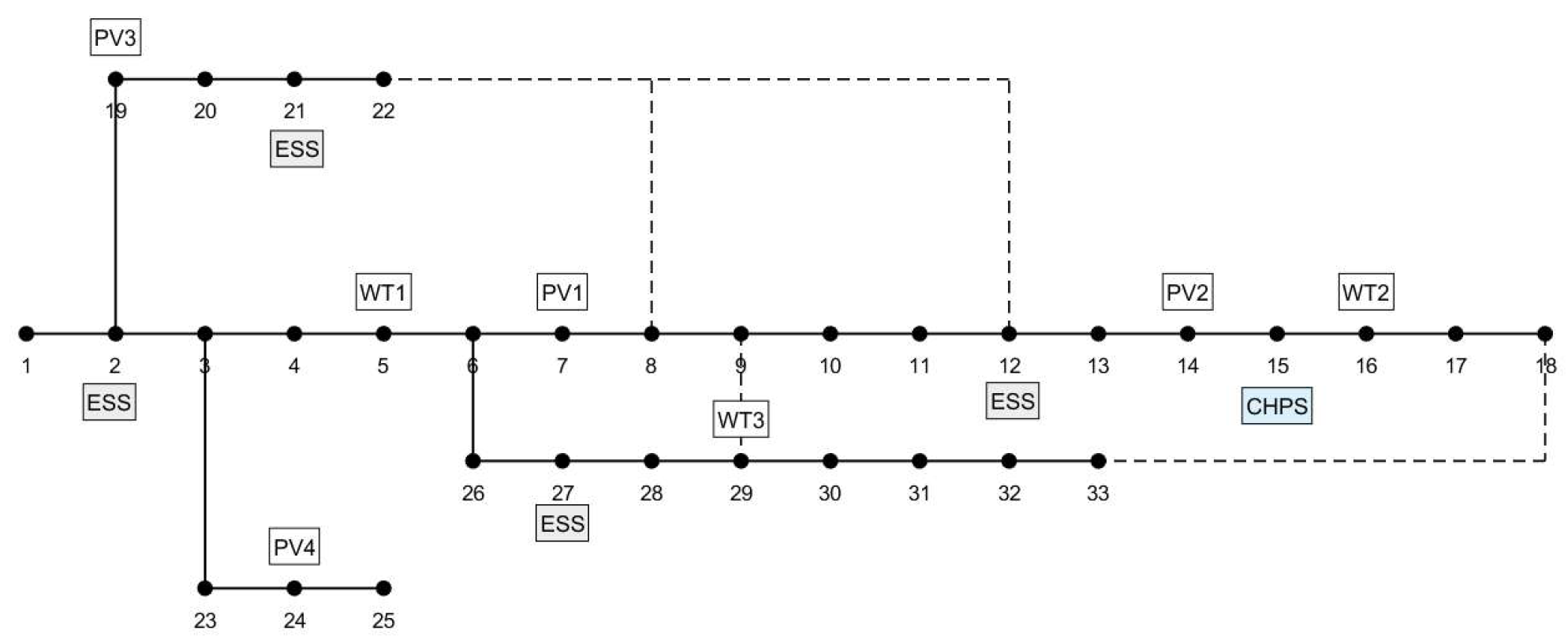
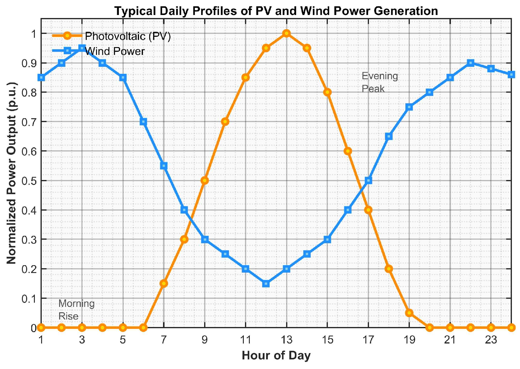
This paper conducts case studies on a modified IEEE 33-bus radial distribution system. A two-reservoir cascade hydropower station is integrated into Bus 15, where two hybrid pumped storage (HPS) units are installed in the upper reservoir (H1) to form an integrated hybrid power plant incorporating both conventional hydropower generation and pumped storage functionalities. All critical transmission lines retain their original power transfer ratings to align with practical grid operation constraints. Distributed energy resources are deployed as follows: PV stations with rated capacities of 4.5 MW, 3.5 MW, 3.5 MW, and 5.5 MW are connected to Buses 7, 14, 19, and 24, respectively; wind farms with installed capacities of 7.0 MW, 5.0 MW, and 6.0 MW are deployed at Buses 5, 16, and 29, respectively; electrochemical energy storage (ESS) systems with power ratings of 3.5–4.5 MW and energy capacities of 7.0–9.0 MWh are configured at Buses 2, 12, 21, and 27. The operational strategies of the distributed ESS units are governed by the energy balance and SOC constraints introduced in Section 3.4, ensuring that their charge/discharge cycles adhere to the defined efficiencies and self-discharge rates. Figure 5 presents the modified IEEE 33-bus distribution system. The basic parameters of all hydropower units in the hybrid system are provided in Table 2 and Table 3. The typical daily output profiles of PV and wind power are presented in Figure 6. The cascade hydro and HPS stations correspond to actual facilities in a regional grid in Northwest China, while wind, PV, and the modified IEEE 33-bus topology are illustrative placements; raw data (2022, hourly) are from that grid’s operational records. The modified IEEE 33-bus system is a representative regional feeder; the relatively large hydro/HPS capacities reflect the real cascade station topology under study.

To ensure reproducibility, the raw hourly demand and renewable generation data used in this study are sourced from the historical operational records of a provincial power grid in Northwest China for the year 2022, with a temporal resolution of 1 h (8760 data points in total). The normalized day profile is constructed using a two-step statistical technique. First, arithmetic averaging is applied to the 365 daily profiles to obtain a typical 24-h mean curve for each hourly timestamp. Second, min-max normalization is performed to scale the profile to a per-unit basis between 0 and 1. While this compression into a single normalized day effectively captures the critical intra-day peak-demand events and the intermittent nature of renewables for evaluating the proposed intra-day optimization strategy, it is acknowledged that multi-day seasonal extremes are smoothed. The multi-day energy storage dynamics are inherently constrained by the SOC and reservoir level limits (Equations (12)–(17) for HPS and Equations (18) and (19) for ESS), ensuring robust operation within the simulation horizon.

Figure 5. IEEE 33-bus distribution system.

Figure 5. IEEE 33-bus distribution system.

Figure 6. The typical daily output profiles of PV and wind power.

Figure 6. The typical daily output profiles of PV and wind power.

4.2. Operational Analysis of the Source-Grid-Load-Storage System with Hybrid Pumped-Storage Cascaded Hydropower Plant

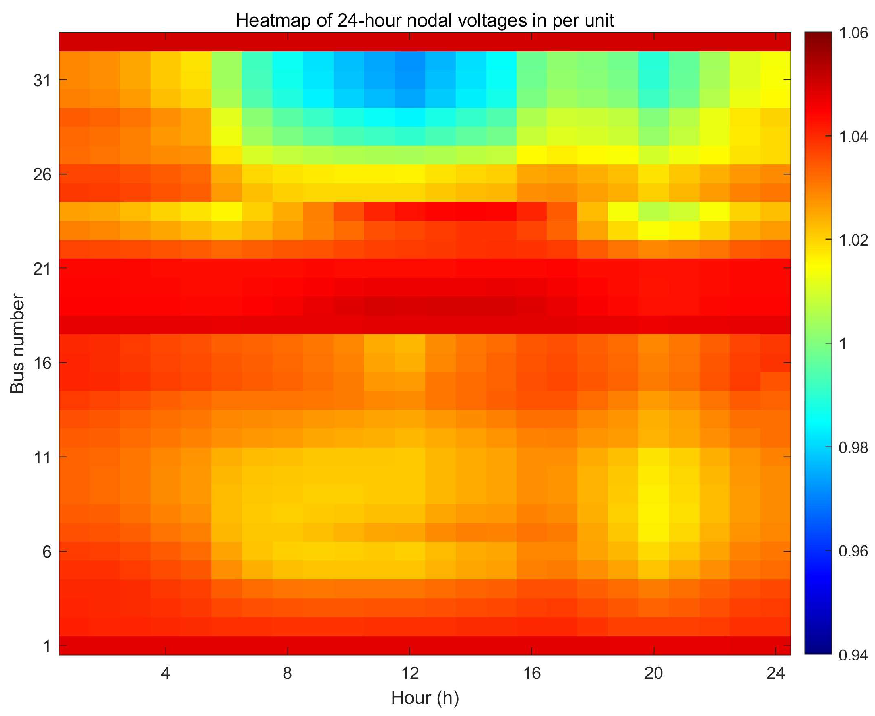
The 24-h nodal voltage heatmap presented in Figure 7 demonstrates that the vast majority of buses in the modified IEEE 33-bus system maintain voltages within the 0.95–1.05 p.u. secure operational envelope throughout the simulation period. Transient minor voltage depressions, dipping to ~0.94 p.u., are only observed at fringe feeder terminals during midday and evening peak load intervals, but voltages recover rapidly to the compliant range without sustained violation. This stable profile confirms that the dynamic reactive power regulation capability of the hybrid pumped-storage cascaded hydropower plant effectively suppresses voltage fluctuations induced by high-penetration renewable integration.

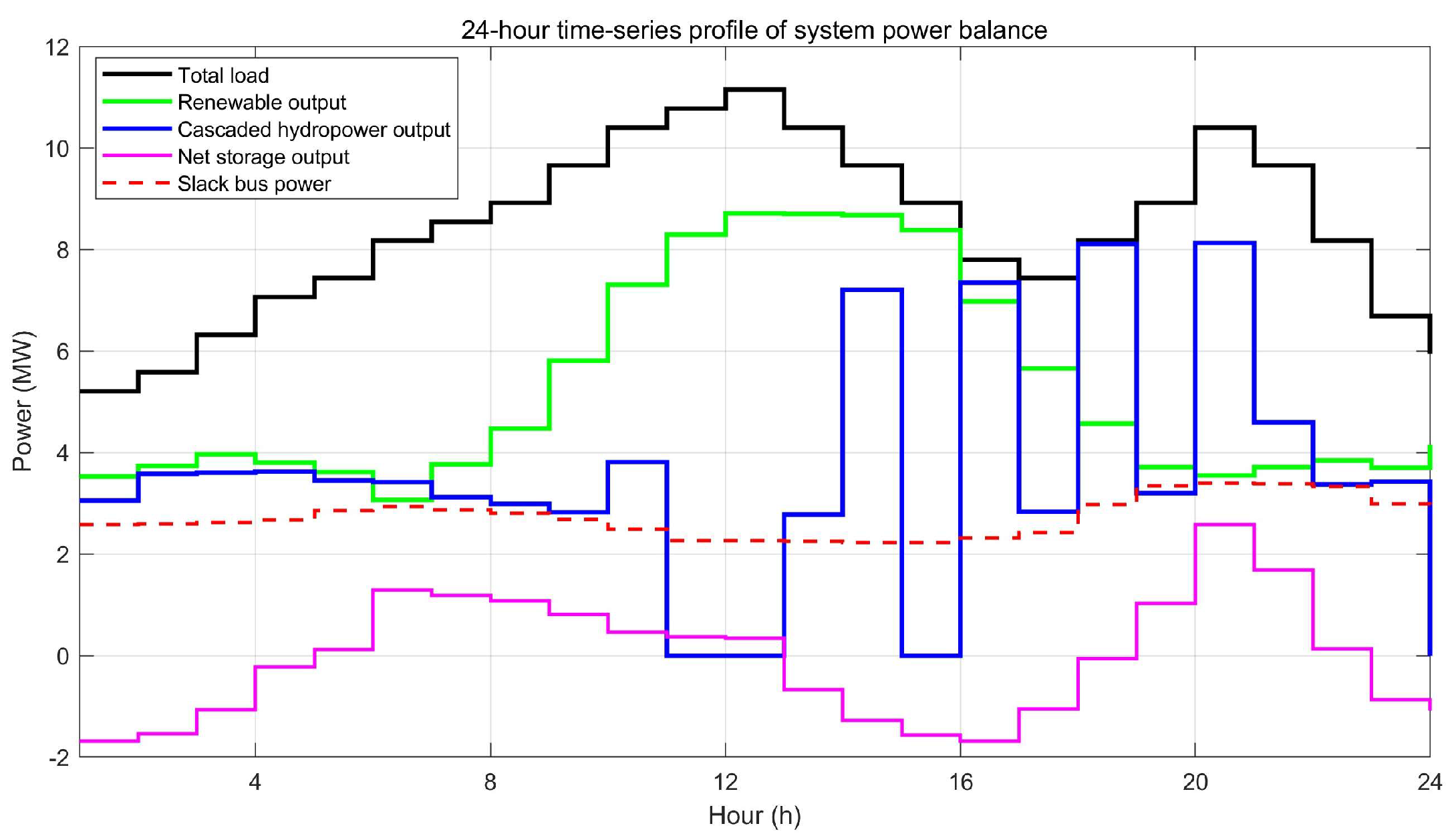
The 24-h power balance timeline in Figure 8 further illustrates how multi-energy complementarity supports full-day supply–demand matching. During daylight hours when photovoltaic output peaks, the hybrid pumped-storage units shift to pumping mode to absorb excess renewable generation, while transitioning to generation mode in the evening to cover the supply gap alongside conventional cascade hydropower units and electrochemical storage systems as load enters its daily peak. Notably, exchange power with the external utility grid remains relatively flat across all intervals, indicating that internal multi-energy synergy meets the majority of the system’s regulation requirements without heavy reliance on external support.

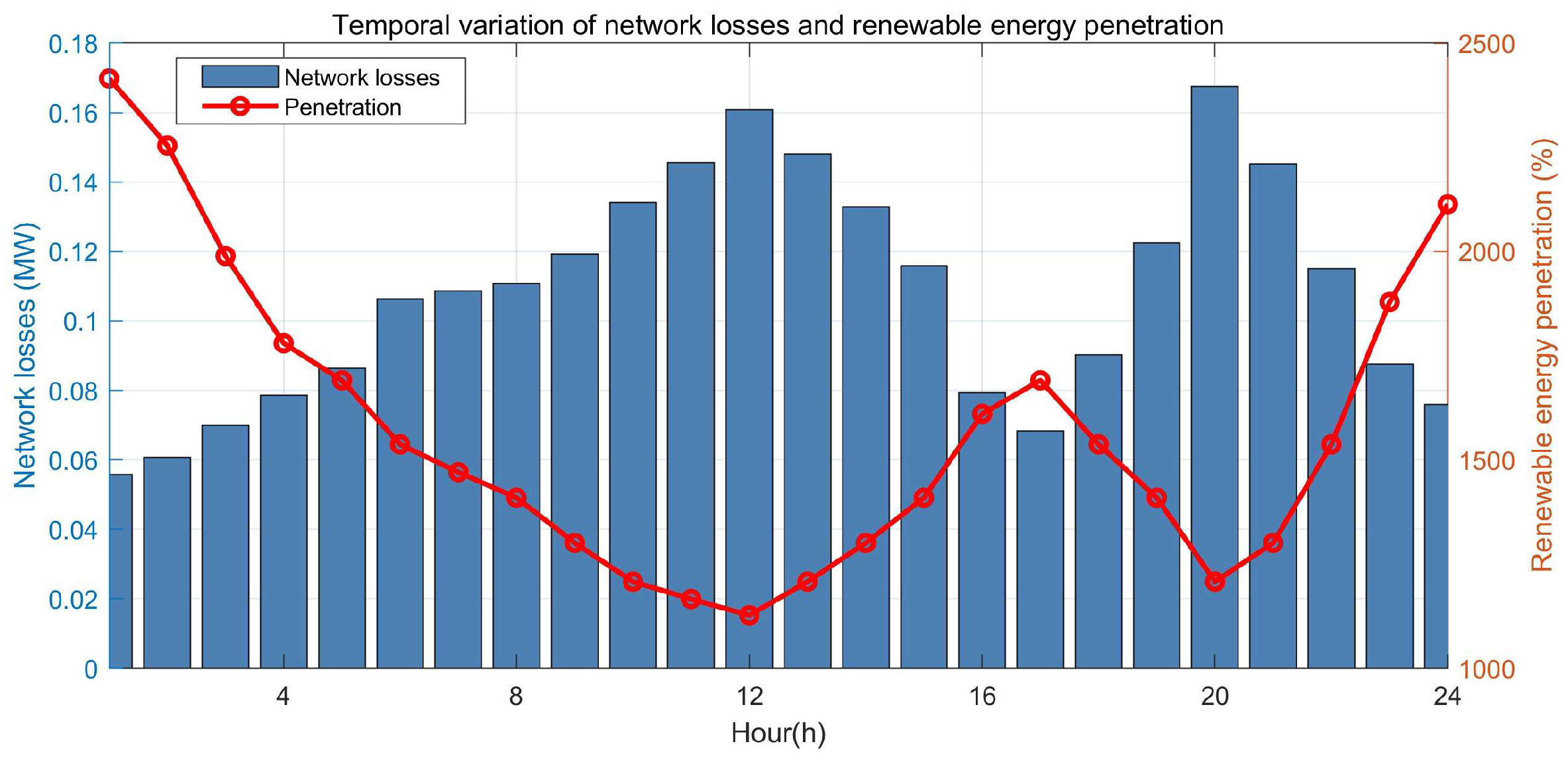
As shown in Figure 9, which tracks temporal variations in system active power losses and renewable energy penetration, the average network active power loss over the 24 h scheduling horizon is 2.59 MW, which corresponds to a total daily energy loss of 62.16 MWh (the same quantity is reported in Table 5); the instantaneous loss is highest around noon, when renewable penetration reaches its maximum and the associated redistribution of power flows aggravates branch loading. The energy-shifting functionality of the pumped-storage units alleviates transmission congestion and keeps the overall losses within an economically viable range. Throughout this paper, the average active power loss is reported in MW, whereas the corresponding daily energy loss is reported in MWh; the two are related by the 24 h duration of the scheduling horizon. Renewable energy accommodation performance is equally robust: photovoltaic generation delivers 61.50 MWh of actual consumption out of 63.33 MWh available, achieving a 97.1% accommodation rate and a corresponding curtailment of 1.83 MWh, while wind power delivers 64.13 MWh out of 77.44 MWh available, reaching an 82.8% accommodation rate and a corresponding curtailment of 13.31 MWh. Because the accommodation rate is defined as the ratio of actual generation to available generation, the total renewable curtailment of the Base Case is 15.14 MWh, which is strictly smaller than the total available wind-and-PV energy of 140.77 MWh and is reported consistently in Table 5. The divergence in accommodation rates stems primarily from inherent output characteristic differences: photovoltaic output aligns closely with daytime load peaks, enabling direct local consumption with minimal need for cross-temporal regulation, while wind power peaks predominantly during nighttime low-load intervals and relies on the pumped-storage units’ energy-shifting capacity to transfer surplus generation to high-demand periods.

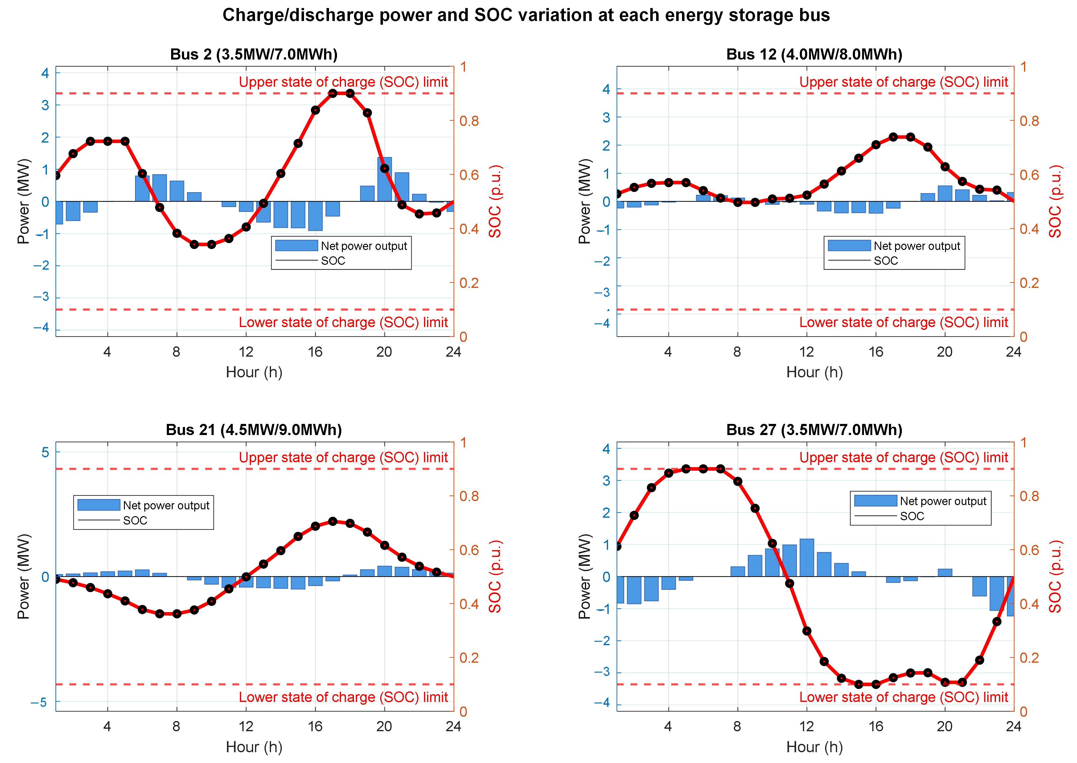
Figure 10 plots the intraday operating profiles of the four distributed energy storage units across the modified IEEE 33-bus system, tracking charge and discharge power alongside state-of-charge evolution. The units adopt differentiated operational strategies aligned with their respective capacity ratings and local load conditions: the 9 MWh unit at Bus 21 maintains a stable, symmetric charge–discharge cycle with its state of charge hovering near 50 percent to provide steady baseline buffering, while the 7 MWh units at Buses 2 and 27 execute more dynamic adjustments, with Bus 27 undergoing deep discharge during daytime peak demand followed by rapid evening recharge to achieve the highest daily energy throughput of 11.72 MWh, and Buses 2 and 12 performing lower-magnitude, higher-frequency tweaks to fine-tune local power balance. Quantitatively, the fleet absorbs 18.13 MWh during charging phases against 16.38 MWh of discharged energy, with the slight net loss consistent with typical storage round-trip efficiency characteristics, and all units strictly adhere to their predefined upper and lower state-of-charge limits throughout the 24-h cycle, validating the feasibility of the coordinated dispatch framework and underscoring the critical role of distributed storage in absorbing surplus renewable generation and smoothing intraday load fluctuations.

4.3. Operational Dynamics of the Hybrid Pumped-Storage Cascaded Hydropower System

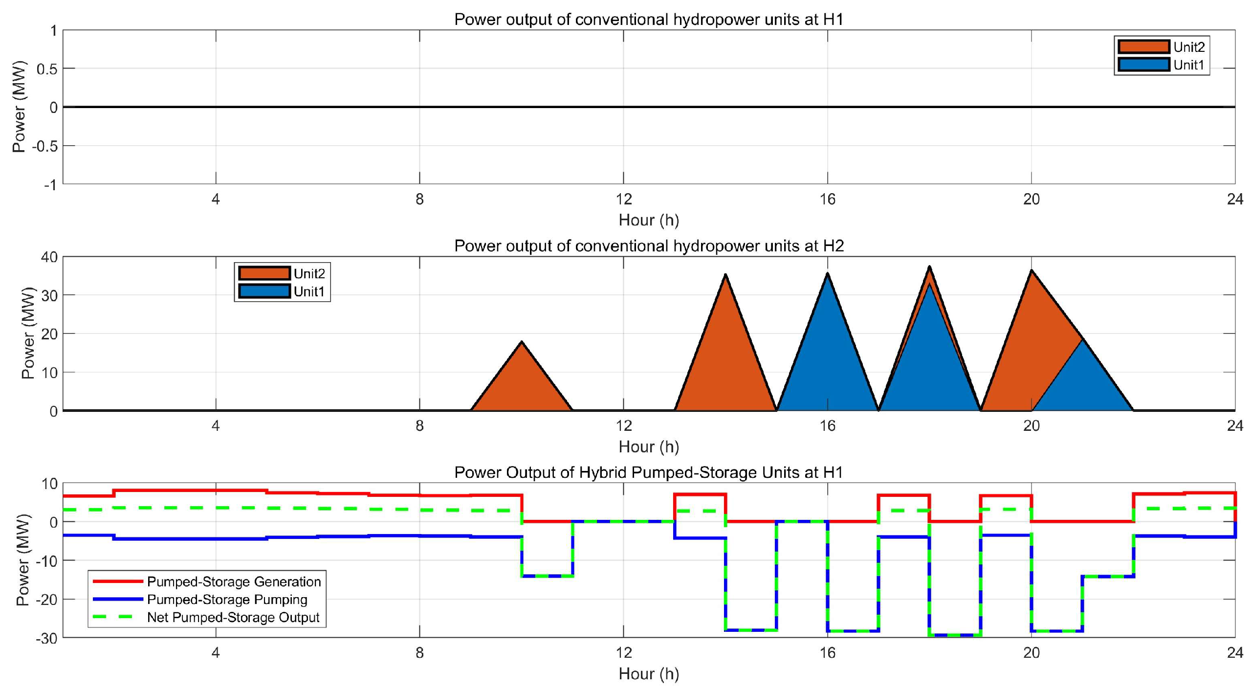
Figure 11 presents the power output profiles of conventional hydropower units at the Stage-I hydropower plant H1 and the Stage-II plant H2, alongside the hybrid pumped-storage units installed at H1. The two H1 conventional units produce no power across the full 24-h scheduling cycle, with no recorded operating intervals. This results from the hierarchical dispatch logic built into the optimization framework, which prioritizes distributed photovoltaic and wind power, downstream H2 conventional units, and hybrid pumped-storage resources over upstream H1 generation. Operational data confirm that H2 units deliver a combined 181.39 MWh of electricity, while the system achieves 97.1% photovoltaic and 82.8% wind power accommodation. The combined capacity of these prioritized resources fully covers diurnal load demand, eliminating the need to activate H1 units for supplementary supply. The H2 units operate across three and four distinct intervals, respectively, averaging 3.66 MW and 3.90 MW, with output profiles aligned to daily load variations that provide stable baseline supply during off-peak periods and flexible mid-load support to complement variable renewable generation, positioning H2 as the core supply source of the cascaded system.

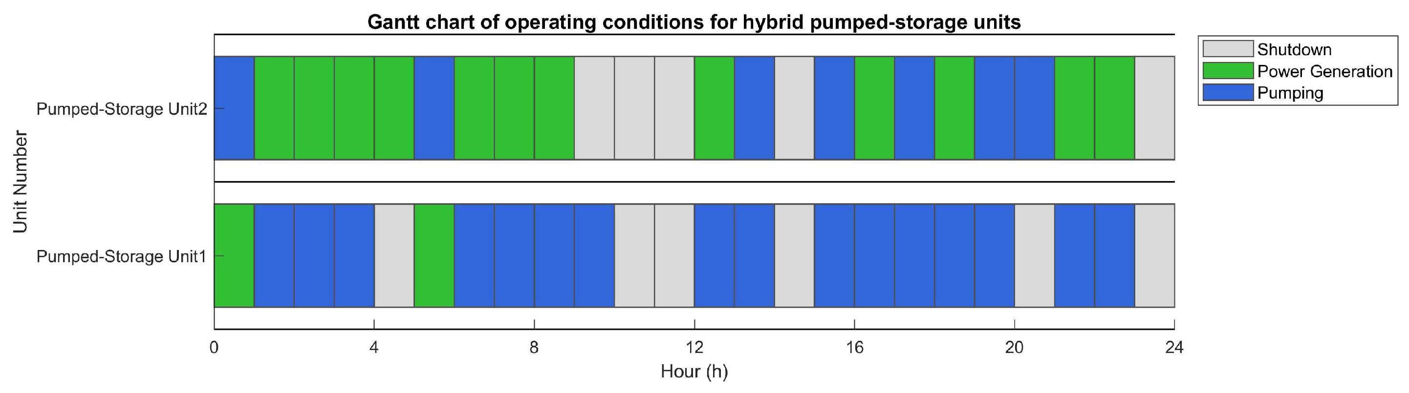
The hybrid pumped-storage units at H1 provide the bulk of the system’s operational flexibility through pronounced bidirectional operation tailored to intraday energy shifting. One unit operates in pumping mode for 17 h, absorbing 121.47 MWh of surplus electricity during midday periods of high renewable output, and generates only 13.88 MWh over two brief intervals, resulting in a net negative output of 107.58 MWh. The second unit balances 12 h of generation producing 87.08 MWh with seven hours of pumping consuming 76.48 MWh, yielding a modest net positive output of 10.60 MWh. Collectively, the hybrid units post a net negative output of 96.98 MWh across the day, functioning primarily as a controllable load to absorb excess renewable energy and store potential energy for later release during peak demand windows. Despite this net negative contribution, the cascaded system as a whole injects 84.41 MWh of electricity into the grid over the 24-h cycle, derived from the sum of H2 conventional generation and net hybrid output. The zero output of H1 conventional units is not an operational anomaly but a deliberate outcome of the cost-minimizing dispatch strategy, which prioritizes lower-marginal-cost resources and maximizes renewable integration. This division of labor, where downstream conventional units provide stable supply, hybrid units manage intraday energy shifting, and upstream conventional units remain as unutilized reserve capacity, enables the system to balance supply reliability, renewable accommodation, and economic efficiency under high renewable penetration scenarios.

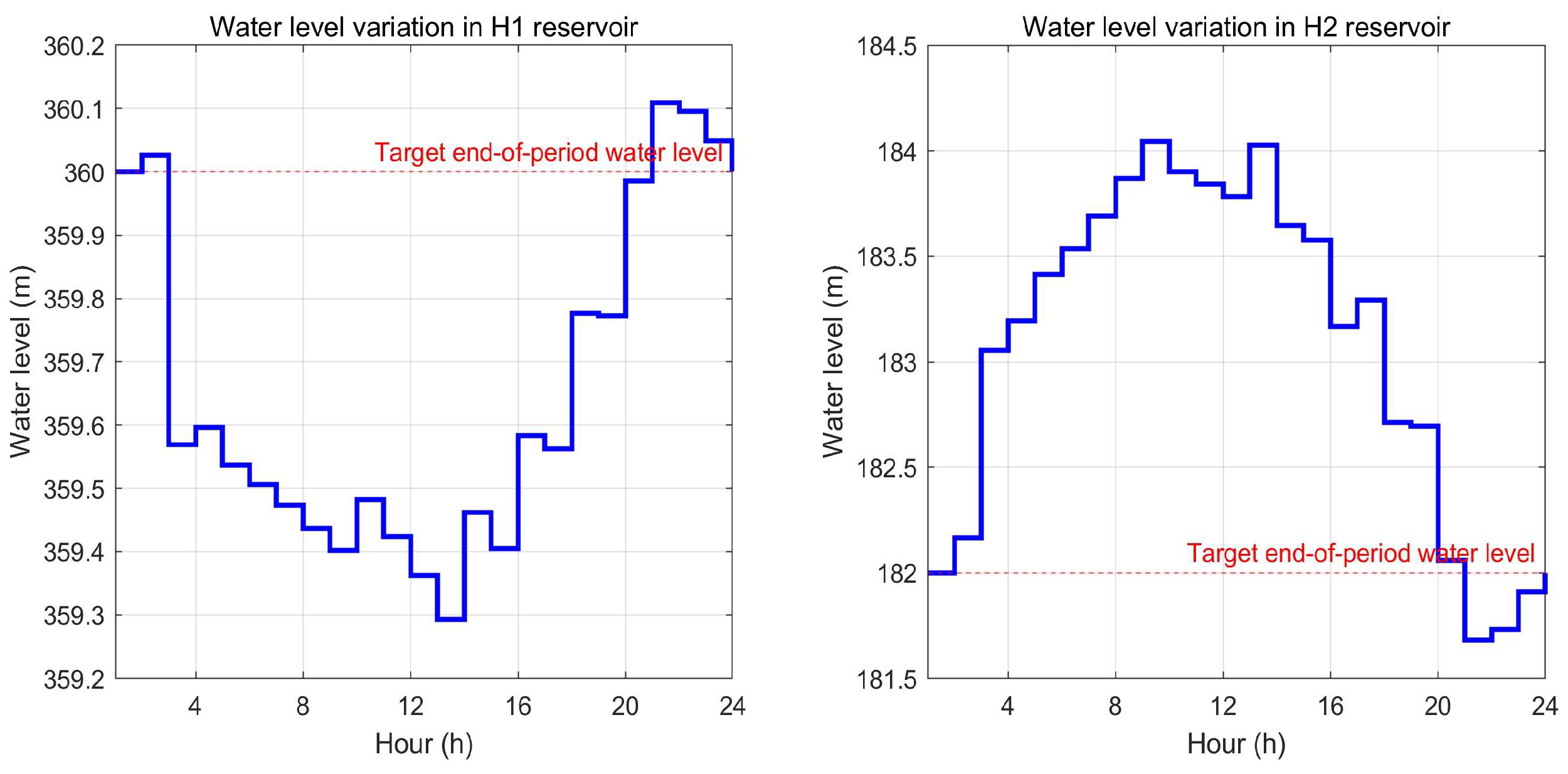
Figure 12 illustrates the daily evolution of water levels in the H1 and H2 reservoirs, demonstrating strict adherence to the periodic storage constraint. The initial and final storage volumes were maintained at 50.00 million m³ for H1 and 40.00 million m³ for H2, respectively; the combined active (regulating) capacity of the two reservoirs is 50 million m³, which is the value used for the spillage normalization in Section 4.5. Despite the closed-loop operation, significant intraday reservoir fluctuations occurred. The H1 reservoir experienced a drawdown from its initial elevation, reaching a minimum level of 359.29 m before recovering to end at 360.11 m. Similarly, the H2 reservoir exhibited a sawtooth pattern, descending to a low of 181.68 m and peaking at 184.04 m. This cyclical variation reflects the dynamic balance between power generation, pumping consumption, and natural inflows managed within the cascaded system.

The Gantt chart of operating conditions for hybrid pumped-storage units is shown in Figure 13. Unit 1 primarily functioned as a net consumer of electricity, engaging in pumping operations for the majority of the pre-peak period, which consumed 121.47 MWh while generating only 13.88 MWh. This resulted in a substantial net negative output of 107.58 MWh. Conversely, Unit 2 adopted a more generation-focused role during the evening peak, producing 87.08 MWh against 76.48 MWh of pumping input, thereby achieving a positive net output of 10.60 MWh. Collectively, the hybrid units facilitated a system-wide net injection while accommodating significant water cycling, as evidenced by the total spillage of 2.45 million m³ at H1 and 2.55 million m³ at H2 (5.00 million m³ in total), underscoring the system’s capability to handle surplus resources efficiently.

4.4. Economic Cost Breakdown of the Proposed System

To validate the cost-minimization objective and demonstrate the economic impact of the proposed scheduling strategy, Table 4 presents a detailed breakdown of the operational costs for the base case (modified IEEE 33-bus system). The results confirm that the objective function, which incorporates comprehensive O&M costs for all assets, provides a transparent representation of the system’s economic performance. A penalty price of 510 USD/MWh is adopted for aL, so that the total curtailed renewable energy of 15.14 MWh in the Base Case yields the curtailment penalty of USD 7721 reported in Table 4.

Table 4. Cost breakdown of the proposed scheduling strategy (unit: USD).

Cost Component	Symbol	Value (USD)
Fuel Cost (Thermal)	Cg	15,917
Start-up & Shut-down Cost	Ck	520
Renewable Curtailment Penalty	Cq	7721
Variable O&M (Hydro/Wind/Solar)	Ch	4727
O&M (Pumped-Storage)	Cp	336
Daily Depreciation (Pumped-Storage)	Cs	17,146
Fixed O&M (Thermal)	Cb	14,400
Total Operational Cost	f1	60,767

Table 4. Cost breakdown of the proposed scheduling strategy (unit: USD).

Cost Component	Symbol	Value (USD)
Fuel Cost (Thermal)	Cg	15,917
Start-up & Shut-down Cost	Ck	520
Renewable Curtailment Penalty	Cq	7721
Variable O&M (Hydro/Wind/Solar)	Ch	4727
O&M (Pumped-Storage)	Cp	336
Daily Depreciation (Pumped-Storage)	Cs	17,146
Fixed O&M (Thermal)	Cb	14,400
Total Operational Cost	f1	60,767

As shown in Table 4, the total 24 h operational cost of the proposed flexible scheduling strategy is 60,767 USD. The dominant cost drivers are the thermal fuel consumption (26.2%) and the daily depreciation of the hybrid pumped-storage asset (28.2%), followed by the fixed O&M of thermal units (23.7%). The inclusion of the renewable curtailment penalty (12.7%) explicitly reflects the economic value of accommodating wind and solar power (achieving PV and wind accommodation rates of 97.1% and 82.8%, respectively). Variable O&M costs for hydro, wind, and solar assets (7.8%) and HPS O&M (0.6%) represent the necessary operational burden of maintaining system flexibility. This full-cost basis-including the fuel, start-up, curtailment penalty, variable O&M, HPS O&M, daily depreciation and fixed O&M terms-is used identically for the operating cost reported in Table 5 of Section 4.5, so that the Base Case entry of USD 60,767 in Table 5 is exactly the objective value f1 detailed in Table 4.

4.5. Comparative Scenario Analysis

To explicitly validate the main contributions of this paper, three distinct scheduling scenarios are established and compared, with the results summarized in Table 5.

The Base Case represents the proposed strategy, incorporating both the allowable reservoir water-level fluctuation range and HPS units. The Fixed-Level Case employs a conventional rigid terminal-water-level constraint (i.e., the allowable fluctuation range is set to zero) while retaining HPS. The Without-HPS Case applies the proposed allowable fluctuation range but deactivates all HPS units to evaluate their standalone impact.

Table 5. Comparative performance of different scheduling scenarios (the operating cost adopts the same full-cost definition as Table 4).

Scenario	Operating Cost (USD)	Renewable Curtailment (MWh)	Reservoir Deviation (m)	Spillage (million m3)	System Losses (MWh)	CO2 (t)	Emission Intensity (kg/MWh)
Base Case (Proposed)	60,767	15.14	0.15	5.00	62.16	185.4	579
Fixed Terminal-Water-Level (+HPS)	81,125	24.50	0.00	3.20	71.0	241.7	628
Without HPS (allowable range)	108,044	35.05	0.18	9.50	96.0	321.5	618

Table 5. Comparative performance of different scheduling scenarios (the operating cost adopts the same full-cost definition as Table 4).

Scenario	Operating Cost (USD)	Renewable Curtailment (MWh)	Reservoir Deviation (m)	Spillage (million m3)	System Losses (MWh)	CO2 (t)	Emission Intensity (kg/MWh)
Base Case (Proposed)	60,767	15.14	0.15	5.00	62.16	185.4	579
Fixed Terminal-Water-Level (+HPS)	81,125	24.50	0.00	3.20	71.0	241.7	628
Without HPS (allowable range)	108,044	35.05	0.18	9.50	96.0	321.5	618

Note to Table 5: the operating cost is the total daily operational cost f1 of Equation (1) and is reported on the same full-cost basis as Table 4; the daily depreciation of the HPS asset is retained in all three scenarios because it is a sunk cost of the already-installed equipment. The renewable curtailment is the sum of curtailed PV and wind energy over the 24 h horizon and is therefore strictly smaller than the total available wind-and-PV energy of 140.77 MWh. The system losses are reported as the total daily energy loss in MWh, whereas the value of 2.59 MW quoted in Section 4.2 and in Section 5 is the corresponding average active power loss.

As shown in Table 5, the Base Case achieves the lowest total operating cost (60,767 USD) and the lowest renewable curtailment (15.14 MWh), confirming the synergistic benefit of combining the allowable fluctuation range with HPS. Compared with the Fixed-Level Case, the Base Case reduces operating cost by 33.5% and curtailment by 38.2%. This is because the rigid terminal constraint in the Fixed-Level Case sacrifices dispatch flexibility—forcing the reservoir level to match the target exactly at each terminal hour—which leads to excessive thermal ramping and renewable curtailment. Its reservoir deviation is strictly zero, but at the expense of significantly higher operational costs. Notably, the Fixed-Level Case exhibits the lowest spillage (3.2 million m³), as the strict water-level enforcement leaves less room for water release; however, this marginal spillage saving is far outweighed by the cost and curtailment penalties.

When compared with the Without-HPS Case, the Base Case reduces operating cost by 43.8% and curtailment by 56.8%. The absence of HPS removes the critical intra-day energy-shifting capability, forcing the system to rely more heavily on thermal generation (520 MWh versus 320 MWh in the Base Case), which substantially increases both fuel cost and network losses (96.0 versus 62.16 MWh). The Without-HPS Case also suffers the highest spillage (9.5 million m³) and reservoir deviation (0.18 m), as cascade hydropower alone cannot flexibly absorb surplus wind and solar power during off-peak periods. As shown in Table 5, the Base Case achieves the lowest CO₂ emissions and emission intensity, confirming the claimed low-carbon benefit of the proposed strategy.

To provide better context for the reported reservoir spillage, the absolute value is normalized against the total annual inflow and the total reservoir capacity. In the Base Case, the total spillage is 5.0 million cubic meters. Considering the total annual inflow of 1200 million cubic meters and the combined active capacity of the cascade reservoirs of 50 million cubic meters, the spillage-to-inflow ratio is 0.42% and the spillage-to-capacity ratio is 10%. Although the absolute spillage may appear large, its relative magnitude is moderate, confirming that the proposed scheduling framework effectively utilizes the majority of incoming water for power generation and grid support. Regarding water-resource sustainability, the proposed allowable reservoir water-level fluctuation range and the integration of hybrid pumped storage (HPS) yield positive implications. Compared to the Fixed-Level Case (3.2 million cubic meters) and the Without-HPS Case (9.5 million cubic meters), the Base Case achieves a balanced spillage level that avoids both excessive water waste and unnecessary reservoir depletion. The HPS units further mitigate spillage by absorbing surplus water through pumping during off-peak periods, converting it into stored potential energy rather than releasing it downstream.

In terms of accommodation, the Base Case achieves wind and solar accommodation rates of 82.8% and 97.1%, respectively, closely matching the values reported in Section 4.2 and validating the effectiveness of the proposed framework. These comparative results underscore that the synergy between the allowable water-level fluctuation range and HPS is essential: the former preserves dispatch feasibility while respecting long-term reservoir boundaries, and the latter provides the flexible regulation resource needed to minimize renewable curtailment and system losses.

5. Conclusions

This paper addresses the operational challenges of cascade hydropower systems under high renewable penetration by proposing an optimal day-ahead scheduling strategy for a cascade hydro-wind-solar-thermal-storage system incorporating hybrid pumped storage (HPS). Targeting the limitations of conventional day-ahead frameworks—including rigid end-of-period reservoir level constraints and insufficient consideration of unit vibration zone restrictions—this study introduces an allowable reservoir water level fluctuation range to balance short-term dispatch flexibility with long-term water resource management requirements. The proposed mixed-integer linear programming (MILP) model coordinates heterogeneous resources, including conventional cascade hydropower, HPS units, variable renewable energy, thermal power units, and distributed energy storage, to minimize total system operation costs while maximizing renewable energy accommodation.

(1)

The integration of HPS significantly enhances the system’s renewable accommodation capacity. The dispatch strategy achieves a 97.1% photovoltaic accommodation rate and an 82.8% wind power accommodation rate. By relaxing rigid end-of-period water level constraints via the allowable fluctuation range, the model avoids infeasibility caused by excessive water level limitations while remaining compliant with medium-to-long-term reservoir operation rules. The cost-minimizing dispatch logic prioritizes low-marginal-cost resources, leaving upstream H1 conventional units offline as standby reserves, which further reduces unnecessary operational expenditures.

(2)

A clear division of labor among system components supports stable day-ahead operation. Downstream H2 conventional units act as the primary baseload suppliers, contributing 181.39 MWh of generation, while HPS units provide core flexibility via bidirectional operation: Unit 1 operates predominantly in pumping mode to absorb surplus midday renewable energy, and Unit 2 balances generation and pumping to support evening peak demand. The coordinated operation yields a net system injection of 84.41 MWh into the grid. Distributed energy storage units at four buses adopt differentiated charge–discharge strategies aligned with local load conditions, which work in tandem with HPS to maintain nodal voltages within the 0.95–1.05 p.u. secure envelope and limit the average network active power loss to 2.59 MW, which is equivalent to a total daily energy loss of 62.16 MWh.

(3)

The allowable water level fluctuation range offers a practical pathway to resolve the conflict between short-term dispatch flexibility and long-term water resource sustainability. While the case study records notable spillage at both H1 and H2 reservoirs due to high natural inflows, the dispatch strategy prioritizes renewable accommodation over strict water conservation, aligning with the low-carbon transition goals of modern power systems.

Future work will focus on refining spillage penalty mechanisms to better balance renewable integration benefits and water resource utilization efficiency, as well as extending the framework to account for multi-scenario renewable output uncertainties within the day-ahead scheduling cycle. Furthermore, while this study embeds key regulatory constraints (e.g., ramp-rate limits, reserve mandates) into the day-ahead scheduling framework, it primarily focuses on the deterministic day-ahead horizon. Future research will extend the model to incorporate stochastic real-time dispatch and explicit market settlement mechanisms for ancillary services, further bridging the gap between scheduling strategies and evolving regulatory policies for hybrid pumped storage systems.

References

1. Zhang, J.; Cheng, C.; Yu, S.; Shen, J.; Wu, X.; Su, H. Preliminary feasibility analysis for remaking the function of cascade hydropower stations to enhance hydropower flexibility: A case study in China. Energy 2022, 260, 125163. [Google Scholar] [CrossRef] [Scilit]
2. Yuan, L.; Liu, H.; Lu, Y.; Zhou, C.; Zhou, C.; Lu, Y. Multi-objective integrated decision method of cascade hydropower stations based on optimization algorithm and evaluation model. J. Hydrog. 2024, 638, 131533. [Google Scholar] [CrossRef] [Scilit]
3. Li, R.; Zhu, G.; Lu, S.; Meng, G.; Chen, L.; Wang, Y.; Huang, E.; Jiao, Y.; Wang, Q. Effects of cascade hydropower stations on hydrologic cycle in Xiying river basin, a runoff in Qilian mountain. J. Hydrog. 2025, 646, 132342. [Google Scholar] [CrossRef] [Scilit]
4. Lu, Y.; Guo, A.; Chang, J.; Wang, Y.; Wang, X.; Niu, C.; Zhang, S.; Xie, Z.; Wang, J. Enhancing the economic benefits of cascade hydropower stations through integrated utilization of electricity and capacity benefits. Energy 2025, 340, 139214. [Google Scholar] [CrossRef] [Scilit]
5. Ren, P.; Zhou, J.; Mo, L.; Zhang, Y. Comprehensive study on cascade hydropower stations in the lower reaches of Yalong river for power generation and ecology. Energy Sustain. Dev. 2023, 73, 236–246. [Google Scholar] [CrossRef] [Scilit]
6. Guo, Y.; Ming, B.; Huang, Q.; Wang, Y.; Zheng, X.; Zhang, W. Risk-averse day-ahead generation scheduling of hydro–wind–photovoltaic complementary systems considering the steady requirement of power delivery. Appl. Energy 2022, 309, 118467. [Google Scholar] [CrossRef] [Scilit]
7. Jiao, Y.; Yang, P.; Jia, R.; Meng, J.; Cao, G.; Guo, Y.; Wen, J.; Månsson, D. Multidimensional evaluation of a wind farm-data center hybrid energy storage system considering full life cycle carbon emissions. Energy 2026, 349, 140696. [Google Scholar] [CrossRef] [Scilit]
8. Du, P.; Ming, B.; Hussain, F.; Fang, W.; Yan, Z.; Yang, X.; Huang, Q.; Liu, P. An explainable deep learning approach for hydropower production forecasting: Evidence from 116 plants in China. Energy 2026, 355, 141237. [Google Scholar] [CrossRef] [Scilit]
9. Wang, K.; Wang, B.; Liang, Z.; Zhou, C.; Ming, B. Hierarchical short-term optimal scheduling of the source-load-storage joint system based on coordinated peak regulation strategy of thermal and energy storage system. J. Energy Storage 2026, 151, 120473. [Google Scholar] [CrossRef] [Scilit]
10. Guo, Y.; Ming, B.; Huang, Q.; Jiang, J.; Yu, M.; San, M.; Cheng, L.; Jia, R. Evaluating the flexibility supply and demand reliability of hydro–wind–PV–battery complementary systems under different consumption modes. Appl. Energy 2025, 379, 124972. [Google Scholar] [CrossRef] [Scilit]
11. Zhu, F.; Zhong, P.-A.; Xu, B.; Liu, W.; Wang, W.; Sun, Y.; Chen, J.; Li, J. Short-term stochastic optimization of a hydro-wind-photovoltaic hybrid system under multiple uncertainties. Energy Convers. Manag. 2020, 214, 112902. [Google Scholar] [CrossRef] [Scilit]
12. Wang, K.; Zhu, H.; Dang, J.; Ming, B.; Wu, X. Short-term optimal scheduling of wind-photovoltaic-hydropower-thermal-pumped hydro storage coupled system based on a novel multi-objective priority stratification method. Energy 2024, 309, 133190. [Google Scholar] [CrossRef] [Scilit]
13. Baghkarvasef, M.; Parvania, M. Integrated artificial intelligence and physics-based modeling for long-term cascaded hydropower scheduling under extreme heat events. IEEE Trans. Sustain. Energy 2025, 17, 590–602. [Google Scholar] [CrossRef] [Scilit]
14. Kang, Y.; Zhao, Z.; Cheng, C.; Wu, X.; Jin, X.; Su, H. Integrating water delay time into short-term hydropower scheduling with spinning reserve capacity allocation and execution. Renew. Energy 2025, 256, 124031. [Google Scholar] [CrossRef] [Scilit]
15. Zhang, Y.; Wang, H.; Fang, G.; Ding, Z.; Huang, X. Optimized scheduling of cascade hydropower stations with advance risk control in dynamic operations. J. Hydrog. 2025, 658, 133196. [Google Scholar] [CrossRef] [Scilit]
16. Bao, Y.; Wang, B.; Li, Y.; Yang, S. Rolling dispatch model considering wind penetration and multi-scale demand response resources. Proc. Chin. Soc. Electr. Eng. 2016, 36, 4589–4600. [Google Scholar] [CrossRef]
17. Zhang, S.; Qiu, G.; Liu, Y.; Ding, L.; Shui, Y. Data-driven distributionally robust optimization based coordinated dispatching for cascaded hydro-PV-PSH combined system. Eng. Sci. Technol. 2023, 55, 128–140. [Google Scholar] [CrossRef]
18. Zhang, Q.; Xie, J.; Pan, X.; Zhang, L.; Fu, D. Short term optimal scheduling model for wind-solar-hydro hybrid power generation system considering dynamic frequency response. Acta Energ. Solaris Sin. 2023, 44, 516–524. [Google Scholar] [CrossRef]
19. Cui, Y.; Zhou, H.; Zhong, W.; Zhao, Y.; Cui, C. Optimal dispatch of power system with energy storage considering deep peak regulation initiative of thermal power and demand response. High Volt. Eng. 2021, 47, 1674–1684. [Google Scholar] [CrossRef]
20. Cui, Y.; Deng, G.; Zeng, P.; Zhong, W.; Zhao, Y.; Liu, X. Multi-time scale source-load dispatch method of power system with wind power considering low-carbon characteristics of carbon capture power plant. Proc. Chin. Soc. Electr. Eng. 2022, 42, 5869–5886+6163. [Google Scholar] [CrossRef]
21. Zhang, R.; Zhang, S.; Wen, X.; Yue, Z.; Zhou, Y. Optimization of short-term hydropower scheduling with dynamic reservoir capacity based on improved genetic algorithm and parallel computing. J. Hydrog. 2024, 636, 131238. [Google Scholar] [CrossRef] [Scilit]
22. Tan, Q.; Nie, Z.; Wen, X.; Su, H.; Fang, G.; Zhang, Z. Complementary scheduling rules for hybrid pumped storage hydropower-photovoltaic power system reconstructing from conventional cascade hydropower stations. Appl. Energy 2024, 355, 122250. [Google Scholar] [CrossRef] [Scilit]
23. Huang, W.; Luo, J.; Ge, L.; He, J.; He, Z.; Wang, X. Consider a generalized economic dispatch strategy combining flexible carbon capture power plants and pumped storage. Proc. Chin. Soc. Electr. Eng. 2024, 44, 1430–1446. [Google Scholar] [CrossRef]
24. Makhdoomi, H.; Moshtagh, J. Optimal scheduling of electrical storage system and flexible loads to participate in energy and flexible ramping product markets. J. Oper. Autom. Power Eng. 2023, 11, 203–212. [Google Scholar] [CrossRef]
25. Li, Y.; Cheng, J.; Li, L.; Shi, Y.; Zhang, D.; Yang, Z.; Chen, N.; An, X. Research on Automatic Power Generation Control and Primary Frequency Regulation Parameter Characteristics of Hydropower Units. Water 2025, 17, 2944. [Google Scholar] [CrossRef] [Scilit]
26. Frew, B.; Brinkman, G.; Denholm, P.; Narwade, V.; Stephen, G.; Bloom, A.; Lau, J. Impact of operating reserve rules on electricity prices with high penetrations of renewable energy. Energy Policy 2021, 156, 112443. [Google Scholar] [CrossRef] [Scilit]
27. GB/T 40595-2021; Guide for Technology and Test on Primary Frequency Control of Grid-Connected Power Resource. Standards Press of China: Beijing, China, 2021.
28. National Energy Administration. Measures for the Management of Electric Power Ancillary Services (Guoneng Fajian Guangui [2021] No. 61). Beijing: National Energy Administration. 2021. Available online: https://zfxxgk.nea.gov.cn/2021-12/21/c_1310391161.htm (accessed on 27 September 2026).
Figure 1. (a) Schematic diagram of a conventional cascade hydropower system. (b) Schematic diagram of a hybrid pumped storage system.
Processes 14 03210 g001
Figure 2. Analysis of hydro-electrical coupling dynamics.
Processes 14 03210 g002
Figure 3. Proposed model architecture diagram.
Processes 14 03210 g003
Figure 4. (a) Energy flow of hybrid pumped storage (HPS). (b) Energy flow of electrochemical energy storage (ESS).
Processes 14 03210 g004
Figure 7. The 24-h nodal voltage heatmap.
Processes 14 03210 g007
Figure 8. The 24-h power balance timeline.
Processes 14 03210 g008
Figure 9. Temporal variation in network losses and renewable energy penetration.
Processes 14 03210 g009
Figure 10. Operating status and SOC regulation of energy storage units at grid buses.
Processes 14 03210 g010
Figure 11. Generation curves of units at H1 and H2, and hybrid pumped-storage at H1.
Processes 14 03210 g011
Figure 12. Daily evolution of water levels in the H1 and H2 reservoirs.
Processes 14 03210 g012
Figure 13. Gantt chart of operating conditions for hybrid pumped-storage units.
Processes 14 03210 g013