Dual-Prior-Constrained Temporal Inversion and FNO Surrogate-Model-Driven Coordinated Optimization of Drilling Engineering Parameters

Abstract

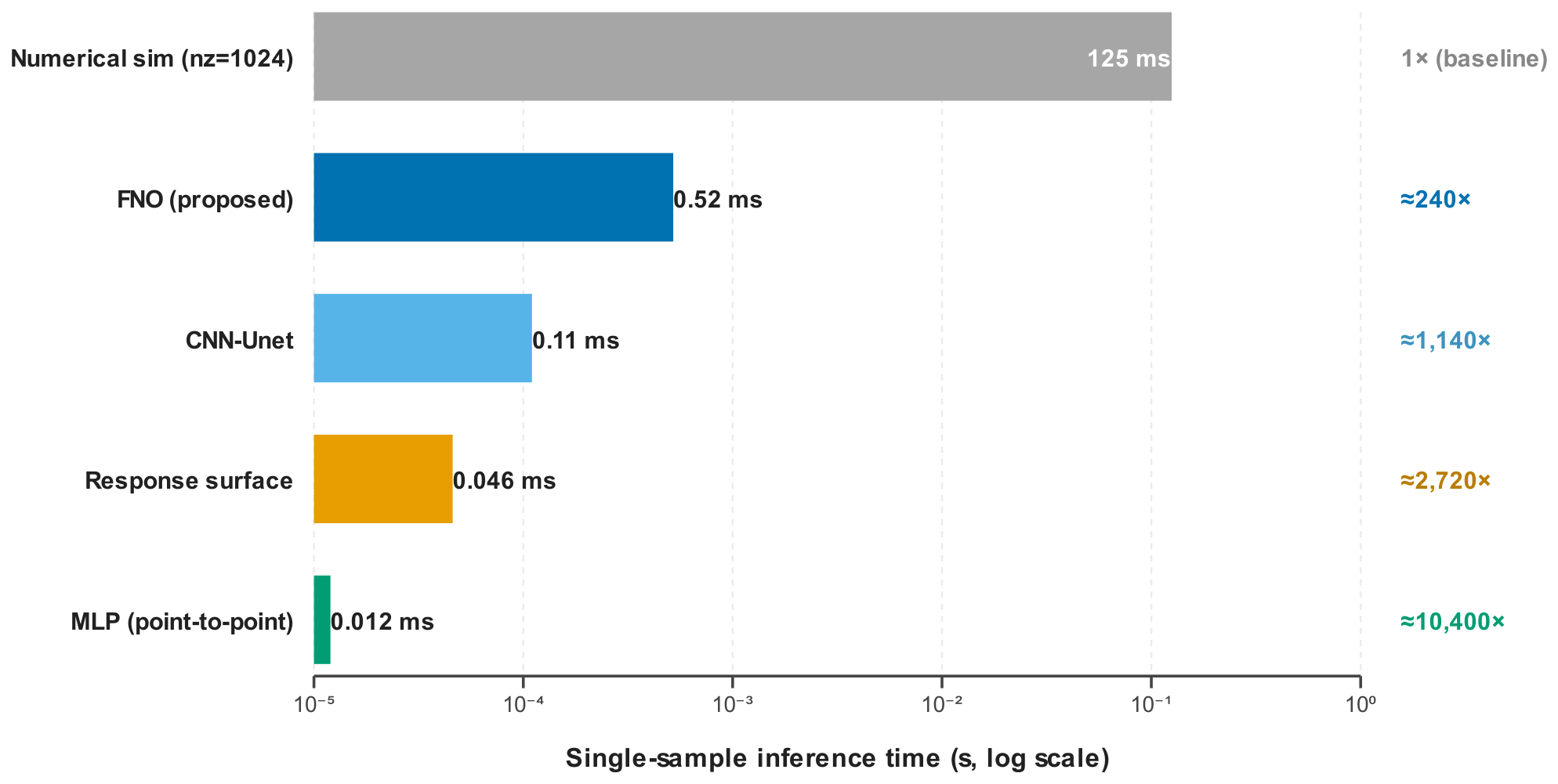
Real-time and accurate inversion of drilling-fluid hydraulic parameters while drilling, together with the coordinated optimization of drilling parameters, is critical for safe and efficient drilling in deep and complex formations. Conventional methods are limited by single-source observations, insufficient prior constraints, weak surrogate-model generalization, and isolated parameter optimization. To address these issues, this paper proposes a three-layer intelligent decision-making framework. The first layer is a dual-prior-constrained temporal inversion module that fuses a pre-drill mechanistic baseline prior with an offset-well statistical prior and estimates plastic viscosity, yield point, annular cuttings concentration, and equivalent eccentricity from standpipe-pressure and rotary-torque observations through a four-term loss function. The second layer is a Fourier neural operator (FNO) surrogate trained on data generated by an in-house two-phase hydraulics solver. All results reported here are obtained on such synthetic data: no field or laboratory measurements are used, and the offset-well statistical prior is prescribed—its mean from a regional depth trend and its covariance from an assumed inter-well variability—rather than fitted to measured offset-well logs. The third layer is a hydraulic–mechanical coupled multi-objective optimization framework that coordinates weight on bit, rotary speed, and flow rate using online Bayesian optimization and probabilistic safety constraints. Numerical experiments with 30 independent noise realizations show that the dual-prior constraints reduce the inversion root-mean-square error by up to 85% for the weakly identifiable parameters (cuttings concentration and equivalent eccentricity) and by 37% for plastic viscosity; that the FNO surrogate is about 240 times faster than the reference numerical simulation and attains a mean relative error of 0.31% for equivalent circulating density and 2.25% for annular pressure loss, about three times lower than the best baseline (a quadratic response surface, 0.95% and 7.16%), preserving that lead outside the training range, while remaining the only surrogate that can be evaluated on a different depth grid without retraining; and that three-parameter optimization improves the rate of penetration by 34.9%. At an equal total surrogate cost, the proposed online optimizer attains the highest mean gain of the methods compared (32.4% over 40 sliding windows, against 31.9% for an online NSGA-II with the same update frequency and 29.4% for a random-search control) while using 4.5 times fewer forward evaluations of the surrogate; the advantage over NSGA-II is small and not statistically resolved at this budget, whereas the advantage over random search is, and the proposed method also has the best worst-case window and the smallest window-to-window spread. The recommended operating points are re-verified with the reference forward solver. Imposing the two analytic closure relations of the forward model as soft physics residuals did not improve accuracy because the reference data satisfy them exactly and the constraint therefore carries no additional information. The framework provides an accurate, efficient, and robust solution for real-time intelligent drilling decision-making.

1. Introduction

With the continuous expansion of oil and gas exploration toward deep, ultra-deep, and structurally complex formations, modern drilling operations are confronted with severe challenges including high-temperature and high-pressure downhole environments, narrow equivalent-circulating-density (ECD) safety windows, and frequent wellbore instability risks [1]. Precise real-time hydraulic monitoring and dynamic parameter optimization are essential to guarantee drilling safety and operational efficiency. Traditional drilling hydraulic analysis and parameter adjustment strategies rely on static pre-drilling design parameters and empirical mechanism models, which fail to capture the dynamic temporal variation of drilling-fluid rheology and annular cuttings transport characteristics during actual drilling processes. Such model errors easily induce downhole complex accidents such as lost circulation, well kick, and borehole collapse [2]. Data-driven early-warning methods for such events are being developed accordingly [3], while characteristic patterns in drillstring mechanics and mud flow measurements can be detected in real time and used as indicators of hazardous intervals [4].

Accurate inversion of downhole hydraulic and cuttings distribution parameters serves as the fundamental premise of real-time while-drilling hydraulic monitoring [5]. Most conventional approaches to managed pressure drilling rely on regulating down-hole pressure to predetermined set points rather than explicitly estimating the magnitude and location of in-/out-flux events through model-based observers [6]. Conventional drilling hydraulics models are typically calibrated offline and become increasingly inaccurate as downhole conditions evolve during drilling, leading to erroneous downhole predictions and elevated operational risk [7]. Although transient models integrated into real-time digital twins have been proposed to monitor downhole cuttings transport, steady-state models still rely on static parameters that fail to capture the dynamic evolution of cuttings distribution [8]. Along-string and wired-pipe measurements now make downhole dynamics available in real time while drilling, and hybrid physics–data schemes use them to estimate bit forces and torque online [9]. Data-driven models trained on laboratory measurements have also been developed to predict the cuttings-bed height directly from operating parameters [10]. Furthermore, existing inversion frameworks underutilize multi-source prior information: pre-drilling mechanism simulation baselines and regional offset-well statistical data, which contain abundant formation and fluid characteristic information, are rarely integrated into inversion constraints, resulting in severe fluctuations and abnormal jumps in inversion results under high measurement noise.

The low computational efficiency of traditional hydraulic forward models constitutes another critical bottleneck restricting real-time drilling intelligent decision-making. Conventional computational fluid dynamics (CFD) methods can achieve high-precision simulation of annular two-phase flow [11,12], yet a single working condition requires hours of iterative calculation, which is incapable of supporting the massive repeated forward evaluations required by online parameter optimization. In recent years, physics-informed neural networks (PINNs) have been applied to fluid-mechanic prediction by embedding physical governing equations into loss functions, enabling physics-driven training that reduces reliance on large labeled datasets [13]. Nevertheless, PINNs remain less accurate than traditional solvers for forward problems [14], although physics-constrained surrogate networks have been shown in simulation to be fast enough to replace the mechanistic model inside a near-real-time control loop for managed-pressure drilling [15]. For complex eccentric rotating annular two-phase flow in drilling engineering, PINNs suffer from difficult training convergence, prominent local prediction errors, and poor adaptability to time-varying drilling conditions, which greatly restrict their practical application in real-time hydraulic prediction.

As an emerging neural-operator architecture, the Fourier neural operator (FNO) implements parametric modeling of integral kernels in Fourier space and directly learns mapping relationships between function spaces, exhibiting advantages of zero-shot super-resolution capability, high computational efficiency, and the ability to learn an entire family of PDEs. Li et al. (2021) originally proposed the FNO framework and showed that it attains higher accuracy than previous learning-based solvers and is up to three orders of magnitude faster than traditional PDE solvers, including on complex turbulent-flow prediction problems [16]. Kovachki et al. (2023) further established the complete theoretical system of neural operators [17]. Nevertheless, the application of FNO in drilling-fluid hydraulic surrogate modeling and drilling-engineering parameter optimization remains underexplored, and its superiority in dynamic drilling prediction and intelligent optimization requires systematic verification [18].

Liu, Ni, and Hui (2026) previously developed a closed-loop machine learning framework integrating real-time lithology identification with drilling parameter optimization, in which optimal WOB and RPM setpoints are derived by inverting the classical Teale MSE model upon formation-change detection [19]; the present study continues this line of work. In terms of drilling parameter optimization, existing studies have explored the optimization of WOB and RPM based on mechanical specific energy (MSE) minimization to improve rock-breaking efficiency [20]. In practical drilling processes, WOB, RPM, and flow rate present strong hydraulic–mechanical coupling and mutually restrictive relationships: WOB and RPM dominate the rate of penetration (ROP) and the cuttings generation rate, whereas the flow rate determines annular pressure loss, ECD variation amplitude, and cuttings carrying efficiency. Isolated single-parameter optimization inevitably deteriorates other drilling performance indicators and fails to achieve a global optimal operational status. Although multi-objective optimization algorithms have been introduced into drilling parameter optimization [21], most existing strategies adopt offline static optimization modes, which cannot dynamically update with real-time variations of downhole formation, fluid, and hydraulic parameters, leading to poor dynamic adaptability and low engineering practicability [22]. A further limitation concerns validation: surrogate-based optimization has been carried out directly on industrial-scale yearly operating data in other process industries [23], and machine learning rate-of-penetration models trained on measured field records have been used to screen operating parameters in drilling [24]. The present study does not reach that stage: no operating data enter any of the three layers, and the validation that a field-deployment claim would require is stated among the limitations.

To address the aforementioned defects in conventional inversion and optimization methods, this paper proposes a novel three-layer stacked intelligent decision framework integrating dual-prior-constrained temporal inversion, FNO hydraulic surrogate modeling, and multi-objective coordinated optimization. The main innovative contributions are summarized as follows:

• A dual-prior-constrained temporal dynamic inversion method is proposed. By integrating pre-drilling mechanism baseline prior and offset-well statistical prior information, combined with standpipe pressure–rotary torque dual observational coupling constraints and sliding-window temporal smooth regularization, a four-term composite loss function is constructed to realize robust real-time inversion of multiple key hydraulic parameters, significantly improving the anti-noise performance and temporal stability of the inversion results.
• An FNO-based eccentric rotating-annular two-phase hydraulic surrogate model is established to replace conventional PINNs. The proposed model realizes full-field hydraulic prediction at sub-millisecond cost and is the only evaluated surrogate whose accuracy is preserved when the depth grid is refined or coarsened without retraining, breaking the efficiency bottleneck of iterative numerical simulation in drilling hydraulic prediction.
• A hydraulic–mechanical coupled three-parameter coordinated real-time optimization framework is constructed to synchronously optimize WOB, RPM, and flow rate. Combined with online Bayesian multi-objective optimization and sliding-window rolling update strategies, dynamic adaptive parameter optimization under time-varying drilling conditions is realized. Probabilistic safety constraints based on inversion-parameter confidence intervals are established to avoid optimization risks induced by parameter uncertainty, achieving a balanced trade-off among drilling safety, efficiency, and energy consumption.

The remainder of this paper is organized as follows. Section 2 first establishes the eccentric rotating-annular two-phase transient hydraulic forward model, then it elaborates the dual-prior-constrained temporal inversion module, the FNO hydraulic surrogate model, and the multi-objective coordinated optimization framework. Section 3 validates the proposed method through numerical simulations, ablation experiments, and comparative analyses, and it provides a discussion of the underlying mechanisms, limitations, and future directions. Section 4 provides a summary of the core conclusions.

1.1. Drilling-Fluid Hydraulic Parameter Inversion

Drilling-fluid hydraulic parameter inversion is a typical ill-posed inverse problem in drilling engineering, aiming to infer unknown downhole fluid rheological properties and annular-flow parameters through measurable surface or downhole observational data. Traditional hydraulic inversion methods primarily rely on steady-state mechanism models and least-squares fitting algorithms, which invert rheological parameters merely based on single standpipe-pressure data. Single-source observational information cannot satisfy the identification requirements of multi-parameter coupled hydraulic systems, resulting in low inversion accuracy and poor stability.

To improve inversion performance, scholars have introduced advanced filtering algorithms and multi-source data constraints into hydraulic-inversion research. He et al. (2022) developed an inversion-based multi-phase-flow interpretation model to realize real-time dynamic identification of downhole flow parameters during managed-pressure drilling [2]. Kaasa et al. (2012) constructed a simplified hydraulic model for high-timeliness downhole-pressure estimation, in which the parameters are updated by recursive online estimation rather than by multi-parameter joint inversion [5]. Hauge et al. (2012) proposed a model-based estimation and control scheme for in/out-flux during managed-pressure drilling [6]. In terms of multi-source-data-fusion monitoring, Arévalo et al. (2022) integrated a transient hole-cleaning model with along-string measurements into a real-time digital twin to track cuttings distribution and reduce borehole-cleaning risk [8].

For the real-time determination of drilling-fluid rheology, Vajargah and van Oort (2015) proposed an approach that estimates downhole rheological properties from distributed pressure measurements, improving the physical rationality of rheology estimation [1]. For online hydraulic-model calibration, Altindal et al. (2025) proposed an online parameter calibration approach that dynamically updates drilling hydraulics models from real-time sensor data by integrating physics-based governing equations with data-driven techniques [7]. Habib et al. (2021) proposed a method for early kick detection and estimation during managed-pressure drilling, including unscented-Kalman-filter-based detection of downhole abnormalities such as gas kick [25].

Nevertheless, existing inversion methods still possess two critical deficiencies. First, most studies exclusively adopt pressure measurements and fail to fully utilize torque signals containing rich rheological and flow-field information, leading to insufficient observational-constraint capability. Second, current prior-constraint strategies are unitary, lacking synchronous integration of mechanism-baseline prior and regional statistical prior information, which results in poor anti-noise performance and temporal stability of inversion results. Different from existing studies, this paper constructs a dual-prior coupled-constraint system based on dual observational data, comprehensively improving the accuracy, stability, and robustness of temporal inversion.

1.2. Fluid Mechanics Surrogate Models and Neural Operators

High-precision CFD numerical simulation is the mainstream approach for drilling-hydraulic-mechanism analysis, whereas its low computational efficiency cannot meet the iterative requirements of online real-time optimization [11]. Surrogate models replace high-cost numerical calculations by constructing input–output mapping relationships of physical systems, serving as an effective solution for efficient hydraulic prediction; they have been used in this way to carry the search loop of well-placement optimization in geothermal reservoirs [26].

Traditional surrogate models such as response-surface methods and Kriging interpolation are typically limited to low-dimensional parameter-space prediction, and their performance degrades when the full flow field is to be reproduced. In recent years, PINNs have become a research hotspot in fluid intelligent prediction owing to their physical-constraint characteristics. Raissi et al. (2019) pioneered the application of PINNs in forward and inverse partial-differential-equation (PDE) solving, providing a novel paradigm for fluid-mechanic intelligent computation [13]. Subsequently, Mao et al. (2020) applied PINNs to high-speed aerodynamic flow modeled by the Euler equations, showing that PINNs perform well on inverse problems but are less accurate than traditional numerical solvers for forward problems [14]. However, PINNs belong to discrete point-to-point-mapping models without resolution invariance, resulting in limited cross-condition generalization and frequent prediction failure under time-varying and boundary working conditions.

Neural operators represented by FNO break through the inherent limitations of traditional neural networks. Li et al. (2021) originally proposed the primitive FNO architecture [16]. Kovachki et al. (2023) systematically proposed neural-operator theories and universal-approximation theorems, verifying the superior performance of FNO in infinite-dimensional-function-space mapping [17]. On this basis, Geo-FNO was developed to adapt complex geometric domains, improving accuracy and discretization convergence for complex-domain computation [27], and physics-augmented variants have been proposed to improve prediction accuracy [28]. At present, FNO has been successfully applied in hydraulic-tomography inversion and subsurface-flow-field prediction [18] and has been reported to outperform convolutional architectures in predicting multiphase flow in fractured reservoirs [29]; yet, to the best of our knowledge, its application in drilling-fluid annular two-phase hydraulic surrogate modeling remains unreported. This paper introduces FNO into drilling-hydraulic prediction and constructs an efficient, resolution-independent surrogate model to support real-time drilling optimization.

1.3. Multi-Objective Optimization of Drilling Parameters

Drilling-parameter optimization is the core approach to coordinate drilling efficiency, operational safety, and energy consumption. Mechanical-specific-energy (MSE) theory provides a quantitative evaluation index for rock-breaking efficiency and is widely applied in WOB and RPM optimization. Nystad et al. (2021) proposed an extremum-seeking-control-based real-time MSE-minimization strategy to realize automatic optimization of mechanical drilling parameters [20]. Closed-loop, model-based automation that adjusts the applied force and the rotary speed online has since been demonstrated in simulation for automated drilling operations [30].

To balance multiple conflicting operational objectives, multi-objective-optimization algorithms have been gradually introduced into drilling-parameter optimization. Song et al. (2022) established a constrained Bayesian multi-objective optimization model that minimizes mechanical specific energy and drilling cost for real-time drilling-parameter optimization [21]. Peng et al. (2023) combined clustering analysis with a deep residual neural network to accurately predict the rate of penetration (ROP) in ultra-deep wells, providing a basis for drilling-parameter optimization [31]. Boukredera et al. (2023) integrated machine-learning models with an optimization algorithm to enhance drilling efficiency and mitigate drill-string vibrations [22].

Existing optimization studies still have prominent limitations. On the one hand, most optimization strategies only optimize single mechanical or hydraulic parameters, ignoring the strong-coupling interactions among WOB, RPM, and flow rate, which cannot achieve global-optimal drilling performance. On the other hand, most optimization methods adopt offline static-solving modes, which fail to dynamically adapt to real-time variations of downhole hydraulic parameters, resulting in poor field adaptability. Targeting the above problems, this paper constructs a hydraulic–mechanical-coupled three-parameter-coordinated online-optimization framework to realize adaptive real-time parameter optimization under time-varying drilling conditions.

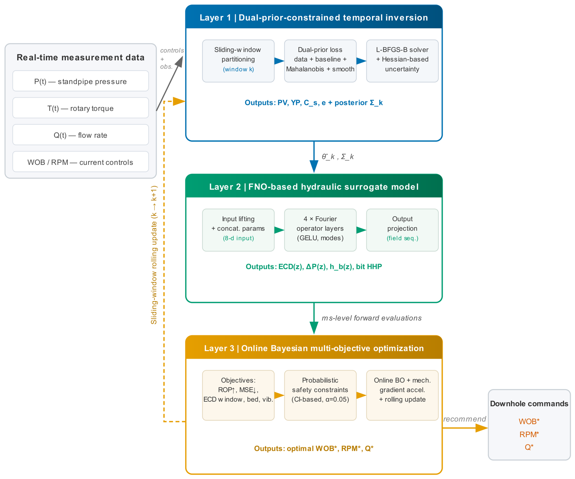
The overall architecture of the proposed three-layer framework is shown in Figure 1: the first layer inverts the hydraulic parameters from the surface measurements, the second layer replaces the reference solver with the FNO surrogate, and the third layer optimizes the drilling parameters online under probabilistic safety constraints taken from the inversion covariance.

2. Methodology

2.1. Basic Assumptions and Governing Equations

This study investigates the drilling-fluid–cuttings two-phase rotating flow in eccentric annuli. The governing equations are established based on the following basic assumptions:

• The drilling fluid is a non-Newtonian fluid conforming to the Herschel–Bulkley (H–B) rheological model.
• Cuttings are treated as a dispersed phase with particle diameters far smaller than the annular clearance, and the Euler–Euler two-fluid model is adopted for description.
• The flow is fully developed axial flow, and the circumferential shear effect induced by drill-string rotation is taken into account.
• The annular eccentricity varies gently along the well depth and is locally regarded as a constant eccentric annular space.
• The cuttings bed forms on the low side of the annulus, and its height is estimated by an empirical model.

The governing equations for annular two-phase flow consist of continuity equations and momentum equations. The continuity equations for the liquid phase (drilling fluid) and the solid phase (cuttings) are, respectively,

$${\displaystyle \frac{\partial \left({\alpha }_l{\rho }_l\right)}{\partial t}}+\nabla ·\left({\alpha }_l{\rho }_l{\mathit{u}}_l\right)=0,$$

(1)

$${\displaystyle \frac{\partial \left({\alpha }_s{\rho }_s\right)}{\partial t}}+\nabla ·\left({\alpha }_s{\rho }_s{\mathit{u}}_s\right)=0,$$

(2)

where ${\alpha }_l$ and ${\alpha }_s$ are the volume fractions of the liquid and solid phases, satisfying ${\alpha }_l+{\alpha }_s=1$; ${\rho }_l$ and ${\rho }_s$ are the densities of the liquid and solid phases; and ${\mathit{u}}_l$ and ${\mathit{u}}_s$ are the velocity vectors of the liquid and solid phases.

The axial momentum equations are

$${\displaystyle \frac{\partial \left({\alpha }_l{\rho }_l{u}_{lz}\right)}{\partial t}}+\nabla ·\left({\alpha }_l{\rho }_l{\mathit{u}}_l{u}_{lz}\right)=-{\alpha }_l{\displaystyle \frac{\partial p}{\partial z}}+\nabla ·\left({\alpha }_l{\mathit{\tau }}_l\right)+{\alpha }_l{\rho }_l{g}_z+M_{ls,z},$$

(3)

$${\displaystyle \frac{\partial \left({\alpha }_s{\rho }_s{u}_{sz}\right)}{\partial t}}+\nabla ·\left({\alpha }_s{\rho }_s{\mathit{u}}_s{u}_{sz}\right)=-{\alpha }_s{\displaystyle \frac{\partial p}{\partial z}}+\nabla ·\left({\alpha }_s{\mathit{\tau }}_s\right)+{\alpha }_s{\rho }_s{g}_z+M_{sl,z},$$

(4)

where p is the pressure; ${\mathit{\tau }}_l$ and ${\mathit{\tau }}_s$ are the viscous stress tensors of the liquid and solid phases; $u_{lz}$ and $u_{sz}$ are the axial velocity components; $g_z$ is the axial component of the gravitational acceleration; and $M_{ls,z}$ and $M_{sl,z}$ are the interphase momentum-exchange terms, satisfying $M_{ls,z}=-M_{sl,z}$.

2.2. Rheological Constitutive Relationship

This study adopts the Herschel–Bulkley (H–B) yield power-law model to describe the constitutive relationship between shear stress and shear rate of the drilling fluid, which serves as the core theoretical basis for hydraulic calculations throughout this paper:

$$\tau ={\tau }_y+K{\dot{\gamma }}^n,$$

(5)

where $\tau$ is the shear stress (Pa); ${\tau }_y$ is the fluid yield stress (Pa, corresponding to the engineering yield point $\mathrm{YP}$); K is the consistency index; $\dot{\gamma }$ is the shear rate; and n is the flow-behavior index (dimensionless).

In the H–B rheological system, the apparent viscosity is a dynamically variable quantity dependent on shear rate rather than the plastic viscosity defined in drilling engineering. To resolve the mismatch between theoretical rheological parameters and engineering measured parameters, and to align with field standard six-speed rotary viscometer testing, this study introduces the industry-standard reference shear rate ${\dot{\gamma }}_0$ and defines the equivalent plastic viscosity:

$$\mathrm{PV}=K{\dot{\gamma }}_0^{n-1}.$$

(6)

In this study, the flow-behavior index n is pre-calibrated by laboratory rheological experiments as a fixed constant and does not participate in the while-drilling inversion calculation. The reference shear rate ${\dot{\gamma }}_0$ is set to the shear rate corresponding to the highest standard viscometer speed of the six-speed rotary viscometer (600 rpm, approximately $1021.7{\mathrm{s}}^{-1}$), so that the equivalent plastic viscosity $\mathrm{PV}$ defined by Equation (6) directly matches the plastic viscosity read from the field six-speed test; in particular, it equals the difference between the dial readings at 600 and 300 rpm for Bingham fluids. The inversion module solves for the two engineering parameters, equivalent plastic viscosity $\mathrm{PV}$ and yield point $\mathrm{YP}$. The consistency index K is then obtained through forward mapping via Equation (6), and combined with the fixed n and the inverted ${\tau }_y$, the three parameters of the H–B model are fully determined. For Bingham fluids ($n=1$), Equation (6) reduces to the classical engineering model, where $\mathrm{PV}=K$ and $\mathrm{YP}={\tau }_y$, fully consistent with drilling industry standard definitions.

Drill-string rotation significantly affects the annular velocity profile through shear-thinning effects and centrifugal forces. The circumferential shear induced by rotation reduces the apparent viscosity, and the equivalent rheological parameters are corrected as

$${\mathrm{PV}}_{\mathrm{eff}}=\mathrm{PV}·f_{\mathrm{rot}}(\mathrm{RPM},e),$$

(7)

$${\mathrm{YP}}_{\mathrm{eff}}=\mathrm{YP}·g_{\mathrm{rot}}(\mathrm{RPM},e),$$

(8)

where $f_{\mathrm{rot}}$ and $g_{\mathrm{rot}}$ are rotation-correction functions related to the rotary speed $\mathrm{RPM}$ and the annular eccentricity e, which are obtained by fitting numerical experiments.

2.3. Correction of Eccentric Annular Velocity Distribution

To obtain an explicit velocity-distribution expression containing spatial coordinates under eccentric geometry, while balancing the nonlinearity of the H–B model and computational efficiency, this study adopts the narrow-slot approximation. Within the local gap, the axial velocity profile is derived using the power-law fluid model (i.e., setting the yield stress to zero); the equivalent consistency index is converted from the inverted $\mathrm{PV}$ through Equation (6). This approximation yields controllable prediction errors for pressure loss and velocity distribution within the engineering-relevant shear-rate range.

The velocity distribution in eccentric annuli differs significantly from that in concentric annuli: the flow velocity is high at the wide gap and low at the narrow gap, causing cuttings to deposit readily on the low side. The local cross-sectional average axial velocity adopts an engineering expression based on the narrow-slot approximation:

$${\overline{u}}_z\left(\theta \right)={\displaystyle \frac{n}{2n+1}}{\left({\displaystyle \frac{\Delta P}{KL}}\right)}^{1/n}{\left(R_2-R_1\right)}^{1+1/n}·h(e,\theta ),$$

(9)

where $R_1$ is the outer radius of the drill string, $R_2$ is the borehole radius, $\Delta P/L$ is the pressure drop per unit length, and $h(e,\theta )$ is the eccentricity-correction function. The eccentricity e is defined as

$$e={\displaystyle \frac{\delta }{R_2-R_1}},$$

(10)

where $\delta$ is the offset distance between the drill-string and wellbore centers. The eccentricity ratio satisfies $e\in [0,1]$; $e=0$ represents a concentric configuration, and $e=1$ represents the drill string contacting the wellbore wall.

Because the training range of Equation (26) reaches $e=0.95$, where the narrow-slot approximation of Equation (9) is least accurate, its error in this range was quantified rather than assumed. A two-dimensional reference solution of the same annulus ($D_h=0.2159$ m, $D_p=0.127$ m) was obtained by solving the axial momentum equation $\nabla ·\left[\mu \left(\dot{\gamma }\right)\nabla u\right]=-G$ with no-slip conditions imposed on the true, non-staircased walls of the eccentric annulus, on Cartesian grids of $N=101$, 201 and 401 nodes, with the flow index of the forward model ($n=0.7$) and its shear-thinning viscosity law. The solver reproduces the exact concentric annular flow rate to $+4.5\%$, $+2.5\%$ and $+1.2\%$ at $N=101$, 201 and 401 (first order in the grid spacing); the two finest grids were combined by Richardson extrapolation to give the reference values below. Drill-string rotation and cuttings transport are absent from the two-dimensional problem, which is consistent with the factorisation of the forward model, where they enter through $f_{\mathrm{rot}}$, $g_{\mathrm{rot}}$ and $F\left(C_s\right)$ rather than through the eccentricity correction.

Table 1. Eccentricity correction of the annular pressure gradient at fixed flow rate, normalized to its value at $e=0.10$, obtained from the two-dimensional reference solution (Richardson extrapolation of the $N=201$ and $N=401$ grids), from the narrow-slot approximation of Equation (9), and from the closure $R_{\mathrm{ecc}}=1-0.35e^2$ used in the forward model. The flow index is $n=0.7$.

e	Two-Dimensional Reference	Narrow-Slot Approximation	Model Closure ${\mathit{R}}_{\mathbf{ecc}}$
0.10	1.000	1.000	1.000
0.25	0.909	0.903	0.982
0.50	0.688	0.669	0.916
0.75	0.492	0.465	0.806
0.90	0.402	0.373	0.719
0.95	0.376	0.347	0.687

compares the eccentricity-induced reduction of the annular pressure gradient at fixed flow rate, normalized to its value at $e=0.10$ so that the concentric baseline cancels and only the eccentricity factor is tested. The narrow-slot approximation tracks the two-dimensional reference closely up to moderate eccentricity—$0.7\%$ at $e=0.25$ and $2.7\%$ at $e=0.5$—and remains within $7.9\%$ at the upper end of the training range ($e=0.95$), where it underestimates the reduction of the pressure gradient, i.e., it overestimates the flow gain produced by the wide gap. The deviation is smaller for a Newtonian fluid of the same geometry ($4.0\%$ at $e=0.95$), so shear thinning amplifies the error of the approximation but keeps it within the accuracy usually accepted for narrow-slot engineering models. The closure actually used for the pressure gradient in the forward model, $R_{\mathrm{ecc}}=1-0.35e^2$, deviates further: it lies $8.0\%$ above the two-dimensional reference at $e=0.25$ and $82.4\%$ above it at $e=0.95$, so the quadratic engineering form underestimates the eccentricity effect at large eccentricity. Because this factor multiplies the annular friction term and the observations are generated with the same closure, the deviation does not bias the self-consistent comparisons of Section 3; what it affects is the absolute level of the annular pressure loss and hence the absolute ECD, which should therefore be read as conditional on the closure. The inverse-crime test of Section 3.2.4 replaces the closure by $\exp (-0.55e^2)$, which differs from the form used here by about $11\%$ at $e=0.95$, and changes the dual-prior errors by at most $0.3\%$, so the inversion is insensitive to a change of closure within this family. The refit itself was also tested directly, the closure being replaced by the two-dimensional reference factor of Table 1 and applied consistently to both the generation of the observations and the inversion operator: the dual-prior results are unaffected by this change (dimensionless overall error of Section 3.2.3: $0.1392$ versus $0.1393$, with the four per-parameter RMSEs agreeing to three significant figures), because the closure cancels between the two roles it plays. What the refit improves is the unconstrained baseline, from $0.557$ to $0.478$, since a stronger eccentricity effect makes e easier to identify without a prior (its RMSE falls from $0.262$ to $0.170$). Every absolute error reported in Section 3 is therefore insensitive to the closure, whereas the relative gain attributed to the priors is mildly sensitive to it: the reduction of the e RMSE, relative to the unconstrained fit, falls from $84.6\%$ to $76.2\%$ under the refitted closure. The quantities that do depend on the closure are the absolute levels—at the top of the inversion envelope ($e=0.64$), the refitted closure lowers the annular pressure gradient by $23\%$ and the peak ECD by 0.069 g/cm³, which is of the same order as the safety margin discussed in Section 3.4.4 and about four times the surrogate-versus-solver deviation reported in Section 3.4.5. Regenerating the labels and retraining the surrogate on the refitted closure, which would shift these absolute levels but no ordering or trend reported here, is left to future work.

2.4. Cuttings Two-Phase Additional Friction and Cuttings Bed Model

The presence of cuttings increases annular flow resistance, and the additional pressure loss is related to the cuttings concentration. A modified two-phase-flow pressure-loss model is adopted:

$${\displaystyle \frac{\Delta P}{L}}={\left({\displaystyle \frac{\Delta P}{L}}\right)}_l·F\left(C_s\right),$$

(11)

where ${(\Delta P/L)}_l$ is the pressure-loss gradient of the pure drilling fluid, $F\left(C_s\right)$ is the cuttings-concentration correction coefficient, and $C_s$ is the average annular cuttings volume concentration.

High-fidelity mechanistic and CFD–DEM studies of annular cuttings transport remain too costly for real-time use, which has motivated data-driven bed-height predictors [10,11,12]; here, the cuttings-bed height $h_b$ is estimated through the cuttings-transport equilibrium relationship:

$$h_b=f(C_s,\mathrm{ROP},Q,\mathrm{PV},\mathrm{YP},d_p,e,{\theta }_{\mathrm{dev}}),$$

(12)

where $d_p$ is the average cuttings particle diameter and ${\theta }_{\mathrm{dev}}$ is the well deviation angle. The presence of the cuttings bed further changes the annular effective flow area and velocity distribution, forming a positive-feedback effect.

2.5. Standpipe Pressure and Rotary Torque Calculation Model

Standpipe pressure is the measured circulating pressure at the drill-floor standpipe during drilling-fluid circulation. The circulating standpipe pressure consists of three dynamic components: the frictional pressure loss inside the drill string, the pressure drop across the bit nozzles due to sudden velocity increase, and the frictional pressure loss in the annulus as the fluid returns to the surface. Because the hydrostatic pressure of the drilling-fluid column on the drill-string side is largely balanced by that of the returning column in the annulus, the net static-pressure difference is negligibly small compared with the dynamic friction components and is therefore not included in the circulating standpipe pressure. Accordingly, the expression for standpipe pressure is

$$P_{\mathrm{standpipe}}=\Delta P_{\mathrm{pipe}}+\Delta P_{\mathrm{bit}}+\Delta P_{\mathrm{annulus}},$$

(13)

where $\Delta P_{\mathrm{pipe}}$ is the frictional pressure loss inside the drill string, $\Delta P_{\mathrm{bit}}$ is the pressure drop across the bit nozzles, and $\Delta P_{\mathrm{annulus}}$ is the frictional pressure loss in the annulus. The standpipe-pressure gauge reading primarily reflects the real-time variations of these three dynamic friction components, which are the quantities relevant to the subsequent hydraulic-parameter inversion.

The rotary torque originates from viscous friction between the drill string and fluid, cuttings-bed friction, and bit–formation interaction. The hydraulics-related torque component can be expressed as

$$T_{\mathrm{hyd}}=2\pi {\int }_0^L{\tau }_w(R_1\left(z\right),z)R_1{\left(z\right)}^2\mathrm{d}z,$$

(14)

where L denotes the total length of the drill string; $R_1\left(z\right)$ represents the outer radius of the drill string, which is piecewise-assigned along the wellbore depth to account for the different diameters of the drill pipe and drill collars; and ${\tau }_w$ denotes the circumferential wall shear stress acting on the outer wall of the drill string, which is closely related to the rheological parameters, the velocity distribution, and the eccentricity.

The above forward model constitutes the physical basis for the inversion and optimization in this study. Among the model parameters, the plastic viscosity $\mathrm{PV}$, yield point $\mathrm{YP}$, average annular cuttings concentration $C_s$, and equivalent eccentricity e are the time-varying parameters to be inverted while drilling, whereas the remaining parameters such as wellbore structure, drill-string dimensions, and cuttings density are known quantities.

2.6. Dual-Prior Constrained Temporal Inversion Module

2.6.1. Problem Formulation and Sliding-Window Mechanism

The objective of while-drilling hydraulic parameter inversion is as follows: given the observed standpipe-pressure sequence $P_{\mathrm{obs}}\left(t\right)$, the observed rotary-torque sequence $T_{\mathrm{obs}}\left(t\right)$, and the flow-rate sequence $Q\left(t\right)$, estimate in real time the four time-varying parameters—plastic viscosity $\mathrm{PV}\left(t\right)$, yield point $\mathrm{YP}\left(t\right)$, average annular cuttings concentration $C_s\left(t\right)$, and equivalent eccentricity $e\left(t\right)$.

Define the parameter vector to be inverted as $\mathit{\theta }\left(t\right)={[\mathrm{PV}\left(t\right),\mathrm{YP}\left(t\right),C_s\left(t\right),e\left(t\right)]}^T$. Because the fluid properties and annular state change relatively slowly during drilling, they can be regarded as quasi-static within a short time window. Therefore, this study adopts a sliding-window mechanism, dividing the continuous time series into fixed windows of length L, within each of which the parameters are treated as constants, and the estimated values are updated window by window.

Let the k-th time window contain N sampling points; the observation vector is

$${\mathit{y}}_k={[P_{\mathrm{obs},1},\dots ,P_{\mathrm{obs},N},T_{\mathrm{obs},1},\dots ,T_{\mathrm{obs},N}]}^T.$$

(15)

The forward model is denoted as $\mathcal{F}({\mathit{\theta }}_k,{\mathit{Q}}_k)$, where ${\mathit{Q}}_k$ is the flow-rate sequence within the window, and its output is the corresponding predicted pressure and torque values. The inversion problem is transformed into an optimization problem within each window:

$${\mathit{\theta }}_k^{*}=\arg \underset{{\mathit{\theta }}_k}{\min }\mathcal{L}\left({\mathit{\theta }}_k\right),$$

(16)

where $\mathcal{L}$ is the total loss function.

2.6.2. Dual-Prior Constraint Design

This study introduces two classes of prior information to constrain the inversion process, constituting a dual-prior constraint mechanism.

First class: pre-drilling mechanism baseline prior. During the drilling design phase, hydraulic simulations are usually performed based on formation prediction and drilling-fluid formulation design to obtain a set of baseline parameters ${\mathit{\theta }}_{\mathrm{base}}$, referred to as the mechanism baseline prior. This prior reflects the physically expected parameter range from the design and serves as the initial baseline and regularization constraint for inversion. The baseline prior adopts an $L_2$ regularization form:

$${\mathcal{L}}_{\mathrm{baseline}}={\parallel {\mathit{\theta }}_k-{\mathit{\theta }}_{\mathrm{base}}\parallel }_2^2.$$

(17)

Second class: offset-well statistical prior. Data from multiple offset wells within the same block contain statistical laws of formation and drilling-fluid characteristics in that region. In this study no measured offset-well data are available, so the prior is prescribed rather than fitted: a regional depth trend supplies the mean and an assumed inter-well variability supplies the covariance, and the resulting multivariate Gaussian distribution is

$$\mathit{\theta }\sim \mathcal{N}({\mathit{\mu }}_{\mathrm{well}},{\mathbf{\Sigma }}_{\mathrm{well}}),$$

(18)

where ${\mathit{\mu }}_{\mathrm{well}}$ is the mean vector of offset-well parameters and ${\mathbf{\Sigma }}_{\mathrm{well}}$ is the covariance matrix. The offset-well prior adopts a regularization term in the form of the Mahalanobis distance, corresponding to the negative log-likelihood of the Gaussian distribution:

$${\mathcal{L}}_{\mathrm{neighbor}}={({\mathit{\theta }}_k-{\mathit{\mu }}_{\mathrm{well}})}^T{\mathbf{\Sigma }}_{\mathrm{well}}^{-1}({\mathit{\theta }}_k-{\mathit{\mu }}_{\mathrm{well}}).$$

(19)

The Mahalanobis distance accounts for correlations among parameters, enabling a more accurate measure of the degree to which the parameters deviate from the block statistical laws.

2.6.3. Four-Term Loss Function

The total loss function consists of four terms, balancing data fitting and prior constraints:

$$\mathcal{L}={\mathcal{L}}_{\mathrm{fit}}+{\lambda }_1{\mathcal{L}}_{\mathrm{baseline}}+{\lambda }_2{\mathcal{L}}_{\mathrm{neighbor}}+{\lambda }_3{\mathcal{L}}_{\mathrm{smooth}}.$$

(20)

Term 1: observation fitting loss. Both standpipe pressure and rotary torque observations are fitted simultaneously, utilizing dual-observation constraints to improve parameter identifiability:

$${\mathcal{L}}_{\mathrm{fit}}={\displaystyle \frac{1}{N}}{\displaystyle \sum _{i=1}^N}\left[w_p{\left({\displaystyle \frac{P_{\mathrm{pred},i}-P_{\mathrm{obs},i}}{P_{\mathrm{obs},i}}}\right)}^2+w_t{\left({\displaystyle \frac{T_{\mathrm{pred},i}-T_{\mathrm{obs},i}}{T_{\mathrm{obs},i}}}\right)}^2\right],$$

(21)

where $w_p$ and $w_t$ are the weighting coefficients for pressure and torque, respectively, set to a nominal (assumed) relative noise level for the two channels rather than calibrated against field measurements, since no field data are used in this study (Section 3.1). The relative-error form is adopted to eliminate dimensional effects.

Term 2: pre-drilling mechanism baseline regularization. As shown in Equation (17), this term constrains the inverted parameters from deviating too far from the design baseline, preventing physically unreasonable results.

Term 3: offset-well statistical prior regularization. As shown in Equation (19), this term constrains the inverted parameters to conform to offset-well statistical laws, improving engineering rationality.

Term 4: temporal smoothness constraint. Parameters in adjacent windows should maintain continuity, suppressing high-frequency fluctuations induced by noise:

$${\mathcal{L}}_{\mathrm{smooth}}={\parallel {\mathit{\theta }}_k-{\mathit{\theta }}_{k-1}\parallel }_2^2,$$

(22)

where ${\mathit{\theta }}_{k-1}$ is the inversion result from the previous window.

Determination of the weights. All three penalty terms are evaluated on dimensionless residuals: the fitting term is already a weighted relative error, and the two prior terms are divided by the characteristic scales $s=(30\mathrm{mPa}·\mathrm{s},10\mathrm{Pa},0.06,0.3)$ for $(\mathrm{PV},\mathrm{YP},C_s,e)$, which are the same scales used to render the parameters comparable in the Mahalanobis distance. The three terms are therefore of comparable magnitude at the solution, so that ${\lambda }_1={\lambda }_2={\lambda }_3=1$—equal weighting in units of the characteristic scales—is the neutral a priori choice, and no further tuning is introduced. This choice was verified rather than assumed: a one-at-a-time sweep of each weight over the range 0 to 10, with the other two held at unity, is reported in Section 3.2.3 and shows that the minimum is a broad plateau that contains unity.

2.6.4. Solution Algorithm and Uncertainty Estimation

Minimization of the loss function is performed using the L-BFGS-B algorithm, which is suitable for small-to-medium-scale bounded optimization problems and exhibits fast convergence. Parameter upper and lower bounds are set according to physical meaning and engineering experience.

To quantify inversion uncertainty, a second-order Taylor expansion of the loss function is performed around the optimal solution, yielding an approximate posterior covariance matrix of the parameters:

$${\mathbf{\Sigma }}_k\approx {\left({\nabla }^2\mathcal{L}\left({\mathit{\theta }}_k^{*}\right)\right)}^{-1},$$

(23)

where ${\nabla }^2\mathcal{L}$ is the Hessian matrix of the loss function. This covariance matrix provides the uncertainty basis for subsequent probabilistic safety-constrained optimization. Note that the fitting loss in Equation (21) is built on weighted relative residuals, and the weighting coefficients $w_p$ and $w_t$ effectively encode the inverse of the observation noise variance. Accordingly, if the observation noise level ${\sigma }^2$ is known explicitly, the posterior covariance in Equation (23) should be scaled as ${\mathbf{\Sigma }}_k\approx {\sigma }^2{\left({\nabla }^2\mathcal{L}\left({\mathit{\theta }}_k^{*}\right)\right)}^{-1}$; otherwise, the un-scaled form may under-estimate the parameter uncertainty by neglecting the noise-induced scale of the fitting residuals. In this study, the weights $w_p$ and $w_t$ are set to a nominal (assumed) observation-noise level rather than calibrated against field measurements, since no field data are involved (Section 3.1); the noise scale is thereby absorbed implicitly, and Equation (23) provides a consistent relative uncertainty estimate. Because the same weights enter the fitting term, they also determine how much information the two observations contribute relative to the priors, and the consequences of this assumption for the identifiability of the parameters and for the safety margins are quantified in Section 3.2.5.

2.7. FNO-Based Hydraulic Surrogate Model

2.7.1. Surrogate Model Positioning and Input–Output Definition

Numerical simulation of eccentric rotating-annular two-phase flow entails enormous computational cost and cannot support the hundreds of online surrogate evaluations required under the sliding-window framework. This study adopts a one-dimensional Fourier neural operator (FNO) to construct a hydraulic surrogate model, learning the solution operator of the parameterized two-phase-flow governing equations and establishing a rapid mapping from rheological parameters and drilling operational parameters to the full-domain hydraulic response along the well depth.

The input vector of the surrogate model is defined as

$$X_{\mathrm{in}}=[\mathrm{PV},\mathrm{YP},C_s,e,\mathrm{WOB},\mathrm{RPM},Q,{\theta }_{\mathrm{dev}}].$$

(24)

The network input is not the bare vector $X_{\mathrm{in}}$ but the field obtained by appending the normalized well-depth coordinate, $u_0\left(z\right)=[X_{\mathrm{in}},z/L]\in {\mathbb{R}}^{n_z\times 9}$, in which the eight physical parameters are broadcast along z. Appending the depth coordinate is essential: without it the input field is constant along z, every non-zero Fourier mode vanishes, and the operator can only return a profile that is constant along the well depth.

The model outputs are one-dimensional discrete sequences along the well depth: the full-domain annular pressure-loss distribution, the equivalent circulating density $\mathrm{ECD}\left(z\right)$, the cuttings-bed height $h_b\left(z\right)$, and the bit hydraulic power sequence.

2.7.2. FNO Network Architecture

This study adopts a one-dimensional FNO architecture adapted to longitudinal well-depth field prediction. The network consists of an input lifting layer, multiple Fourier operator layers, nonlinear activation layers, and an output projection layer:

• Lifting layer: maps the low-dimensional parameter vector to the hidden channel dimension $d_{\mathrm{hidden}}$.
• Fourier operator core layers:

  $${\left(\mathcal{F}u\right)}_k\left(z\right)=\sigma \left(Wu\left(z\right)+{\mathcal{F}}^{-1}\left(R_k\odot \mathcal{F}\left(u\right)\right)\left(z\right)\right),$$

  (25)

  where $\mathcal{F}$ and ${\mathcal{F}}^{-1}$ are the one-dimensional Fourier forward and inverse transforms, $R_k$ is the learnable kernel in Fourier space, ⊙ denotes the Hadamard product, W is the local linear transformation, and the activation function $\sigma$ is chosen as GELU. The model is configured with four Fourier operator layers, $d_{\mathrm{hidden}}=48$ hidden channels and 12 retained Fourier modes, giving 231,219 trainable parameters; the number of retained modes is truncated to balance accuracy and computational cost.
• Output projection layer: maps the high-dimensional hidden features to the hydraulic response field sequences.

2.7.3. Training Dataset Construction

All training samples are generated in batch by the eccentric annular two-phase hydraulic forward model described in Section 2, with parameters covering the engineering-reasonable ranges:

$$\begin{array}{c}\mathrm{PV}\in [10,80]\mathrm{mPa}·\mathrm{s},\mathrm{YP}\in [2,30]\mathrm{Pa},\hfill \\ C_s\in [0,0.15],e\in [0,0.95],\hfill \\ Q\in [15,40]\mathrm{L}/\mathrm{s},\mathrm{RPM}\in [40,180],\hfill \\ {\theta }_{\mathrm{dev}}\in [0°,90°].\hfill \end{array}$$

(26)

The dataset comprises 1200 training samples and 300 test samples (80%/20%); all inputs and outputs are min–max normalized to eliminate training bias caused by different physical dimensions.

Because both the training labels and the test set are produced by the same forward model whose closure relations define the physics of the problem, the errors reported in Section 3.3.1 measure how faithfully the surrogate reproduces that model rather than how faithfully it reproduces a real well: they are a self-consistent upper bound on the accuracy to be expected in the field. Under field conditions, the same network would additionally face a different or transient rheological closure, unmodeled downhole phenomena, and instrument anomalies, so its accuracy should be expected to degrade, and a calibration against field data would be required before operational use. The inversion layer below is subject to the analogous qualification, namely a mismatch between the operator that generates the observations and the operator used to invert them, which is quantified in Section 3.2.4.

2.7.4. Training Loss Function

Training minimizes the mean squared error between the predicted and the reference field, both min–max normalized:

$${\mathcal{L}}_{\mathrm{FNO}}={\displaystyle \frac{1}{N_s}}{\displaystyle \sum _{i=1}^{N_s}}\parallel {\mathit{Y}}_{\mathrm{pred},i}-{\mathit{Y}}_{\mathrm{true},i}{\parallel }_2^2,$$

(27)

where $N_s$ is the number of samples, ${\mathit{Y}}_{\mathrm{pred},i}$ is the hydraulic field predicted by the surrogate model, and ${\mathit{Y}}_{\mathrm{true},i}$ is the numerical-simulation ground truth. Model accuracy is reported with the field-averaged relative $L_2$ error

$$\mathrm{rel}{L}_2={\displaystyle \frac{{\parallel {\mathit{Y}}_{\mathrm{pred}}-{\mathit{Y}}_{\mathrm{true}}\parallel }_2}{{\parallel {\mathit{Y}}_{\mathrm{true}}\parallel }_2+\epsilon }},$$

(28)

computed per output channel over the whole test set, where $\epsilon$ is a tiny constant to avoid division by zero.

The three output fields are not independent: at the fixed point of the reference solver, they are linked by the closure relations of the underlying two-phase annular-flow model. Two of these relations are imposed as soft constraints in the physics-informed variant, giving the loss

$$\mathcal{L}={\mathcal{L}}_{\mathrm{FNO}}+\lambda \left({∥r_{h_b}∥}_2^2+{∥r_{\mathrm{ECD}}∥}_2^2\right),$$

(29)

with the standardized residuals

$$r_{h_b}={\displaystyle \frac{h_b\left(z\right)-\mathcal{H}\left[{\partial }_{z}P\left(z\right)\right]}{s_{h_b}}},r_{\mathrm{ECD}}={\displaystyle \frac{\mathrm{ECD}\left(z\right)-\mathcal{E}\left[{\partial }_{z}P\right]\left(z\right)}{s_{\mathrm{ECD}}}},$$

(30)

where $\mathcal{H}$ is the cuttings-bed equilibrium closure (the equilibrium bed height produced by the local pressure gradient), $\mathcal{E}$ is the depth-accumulation definition of the equivalent circulating density, and $s_{h_b}$ and $s_{\mathrm{ECD}}$ are the standard deviations of the two fields over the training set, which render both residuals dimensionless and comparable in scale to the normalized data term.

The residuals of the three relations on the reference data are reported in

Table 2. Residuals of the three closure relations of the reference forward model, evaluated on 200 randomly sampled parameter sets at $n_z=64$. All three relations are satisfied by the reference data, the momentum and ECD relations identically and the cuttings-bed relation to machine precision.

Closure	Mean Absolute Residual	Relative to Field Std
Momentum, ${\partial }_{z}P=\mathcal{G}\left(h_b\right)$	0 Pa/m	$0\%$
Cuttings bed, $h_b=\mathcal{H}\left({\partial }_{z}P\right)$	$1.2\times {10}^{-13}$ m	$2\times {10}^{-9}\%$
ECD accumulation, $\mathrm{ECD}=\mathcal{E}\left({\partial }_{z}P\right)$	0 g/cm3	$0\%$

. The forward model is solved to the converged coupled fixed point rather than truncated after a fixed number of sweeps: the bed height is obtained by a bisection on the scalar fixed-point equation $h_b=\mathcal{H}\left[\mathcal{G}\left(h_b\right)\right]$, which is well posed because the composite map is monotone decreasing and the two ends of the admissible interval $[0,h_{\max }]$ bracket its root. Once $h_b$ is known, the pressure gradient and the ECD follow from $\mathcal{G}$ and $\mathcal{E}$, so these two relations hold identically by construction, while the bed relation—the one actually solved for—holds to machine precision, at $1.2\times {10}^{-13}$ m, i.e., $2\times {10}^{-9}\%$ of the field standard deviation. Every closure is therefore an identity on the labels, and a residual term evaluated on them vanishes. Whether such a term is nevertheless useful in practice is not a matter of principle but of measurement: the weight $\lambda$ of Equation (29) is swept in Section 3.3.4, where every non-zero value tested is found to degrade the accuracy, and the production surrogate is accordingly trained with $\lambda =0$. This differs from the situation a PINN addresses. In a PINN, the governing equations are the only source of physical information available because the data are sparse, noisy or incomplete; here, the same equations are already imposed upstream, in the generation of the labels, and the residual evaluated on a label is zero by construction, so it can only reshape the loss landscape rather than add information.

The weight $\lambda$ is ramped linearly from zero over the first 15% of the optimization steps and then held fixed. Its value is not a free numerical knob to be tuned for accuracy: as the ablation of Section 3.3.4 shows, the reference data satisfy the closure relations to machine precision, so the residuals vanish on the labels, and the term is found to degrade accuracy at every tested value of $\lambda$. The production surrogate is therefore trained with $\lambda =0$, and the physics-informed variant is retained only as an ablation.

2.7.5. Training Strategy and Online Inference Workflow

The optimizer is Adam with a cosine-decayed learning rate from $5\times {10}^{-3}$ to $1\times {10}^{-4}$, a mini-batch size of 256 and 250 epochs, i.e., 1000 optimization steps; the weights of the final step are retained. Mini-batching is essential at this model size: the earlier full-batch configuration performed only one update per epoch and stalled near the constant-predictor level, whereas the same architecture optimized in 256-sample batches converges to the accuracy reported below.

The real-time inference workflow is as follows:

• Receive the real-time parameters ${\mathit{\theta }}_k$ output from the inversion module described in Section 2.
• Concatenate with the current drilling operational parameters to form the complete input vector.
• Perform the FNO forward pass to output the full-domain ECD, cuttings-bed height, and annular pressure loss in sub-millisecond time.
• Feed the prediction results into the multi-objective optimization module to serve as the rapid evaluation kernel of the objective functions.

2.8. Hydraulic–Mechanical Coupled Multi-Objective Coordinated Optimization Framework

2.8.1. Multi-Objective Optimization Mathematical Model

The decision variables to be optimized are

$$\mathit{x}={[\mathrm{WOB},\mathrm{RPM},Q]}^T.$$

(31)

Objective 1: maximize the rate of penetration ($\mathrm{ROP}$). The rate of penetration is the core indicator of drilling efficiency, and the drillability empirical model applicable to rotary drilling is adopted:

$$f_1\left(\mathit{x}\right)=\mathrm{ROP}=K_d·{\mathrm{WOB}}^{a_1}·{\mathrm{RPM}}^{a_2}·\exp (-\beta V_{\mathrm{risk}}),$$

(32)

where $K_d$ is the formation drillability coefficient, $a_1$ and $a_2$ are fitting exponents, and $\beta$ is the vibration-suppression coefficient. The optimization objective is to maximize $f_1\left(\mathit{x}\right)$.

Objective 2: minimize the mechanical specific energy ($\mathrm{MSE}$). The mechanical specific energy reflects rock-breaking efficiency, defined as the energy required to break a unit volume of rock:

$$f_2\left(\mathit{x}\right)=\mathrm{MSE}={\displaystyle \frac{\mathrm{WOB}}{A}}+{\displaystyle \frac{2\pi ·\mathrm{RPM}·T}{A·\mathrm{ROP}}},$$

(33)

where A is the bottom-hole area and T is the comprehensive bit torque. The optimization objective is to minimize $f_2\left(\mathit{x}\right)$.

Objective 3: ECD safety-window deviation. The equivalent circulating density must be controlled within the safe window between formation pore pressure and fracture pressure. The safety deviation is defined as

$$f_3\left(\mathit{x}\right)=\max \left(0,{\mathrm{ECD}}_{\max }-{\mathrm{ECD}}_{\mathrm{upper}}\right)+\max \left(0,{\mathrm{ECD}}_{\mathrm{lower}}-{\mathrm{ECD}}_{\min }\right),$$

(34)

where ${\mathrm{ECD}}_{\mathrm{upper}}$ and ${\mathrm{ECD}}_{\mathrm{lower}}$ are the upper and lower bounds of the safety window, respectively. The optimization objective is to minimize $f_3\left(\mathit{x}\right)$, whose ideal value is zero.

Objective 4: minimize the cuttings-bed height. Excessive cuttings-bed height can cause stuck pipe and drag issues; the maximum cuttings-bed height along the full well section is taken:

$$f_4\left(\mathit{x}\right)=\underset{z}{\max }{h}_b(z,\mathit{x},\mathit{\theta }).$$

(35)

The optimization objective is to minimize $f_4\left(\mathit{x}\right)$.

Objective 5: minimize the vibration risk. Excessive weight on bit and rotary speed can induce whirl and bit-bounce vibrations; an empirical vibration-risk model is adopted:

$$f_5\left(\mathit{x}\right)=V_{\mathrm{risk}}(\mathrm{WOB},\mathrm{RPM}).$$

(36)

The optimization objective is to minimize $f_5\left(\mathit{x}\right)$.

The constraints include the physical upper and lower bounds of each parameter and the equipment-capacity limits:

$${\mathrm{WOB}}_{\min }\le \mathrm{WOB}\le {\mathrm{WOB}}_{\max },{\mathrm{RPM}}_{\min }\le \mathrm{RPM}\le {\mathrm{RPM}}_{\max },Q_{\min }\le Q\le Q_{\max }.$$

(37)

The multi-objective optimization problem is uniformly converted into minimization form:

$$\underset{\mathit{x}\in \mathsf{\Omega }}{\min }\mathit{F}\left(\mathit{x}\right)={[-f_1\left(\mathit{x}\right),f_2\left(\mathit{x}\right),f_3\left(\mathit{x}\right),f_4\left(\mathit{x}\right),f_5\left(\mathit{x}\right)]}^T,$$

(38)

where $\mathsf{\Omega }$ is the feasible domain.

2.8.2. Online Bayesian Multi-Objective Optimization Algorithm

Traditional black-box multi-objective optimization algorithms such as NSGA-II need a large number of objective-function evaluations per window. In the present framework, those evaluations are surrogate evaluations rather than calls to the reference solver, so they are affordable; the quantity worth reducing is therefore the number of them, which is what the proposed algorithm does. This study adopts an online Bayesian multi-objective optimization algorithm of the ParEGO family, which selects evaluation points through an acquisition function and additionally exploits the analytic gradient of the surrogate to satisfy the ECD constraint. The purpose of that mechanism gradient is to concentrate the limited number of evaluations a sliding window can afford on the constraint surface, where the constrained optimum lies, instead of spending them in the interior of the feasible region. As shown quantitatively in Section 3.4.3, the proposed optimizer reaches the ROP gain of an equally funded online NSGA-II with 4.5 times fewer forward evaluations of the FNO. That evaluation saving is bought with backward passes, and at equal total surrogate cost the advantage over a well-tuned black-box optimizer is not resolved by our experiments; the complete comparison, including the cases in which a black-box search is preferable, is reported in Section 3.4.3 and not concealed here.

Surrogate model. At each sliding window, the multi-objective problem is first scalarized into a single objective by a random-weight augmented Tchebycheff aggregation of the normalized ROP gain and specific-energy objectives, and a Gaussian-process (GP) surrogate with an isotropic radial-basis kernel is then fitted to the scalarized objective over the operating points evaluated so far. The kernel length scale is selected by minimizing the negative log marginal likelihood over a fixed grid. Because two objectives are aggregated into one scalarized objective per window with a random weight drawn from a Dirichlet distribution, a single GP is fitted per window instead of one GP per objective.

Acquisition function. The Expected Improvement (EI) criterion is adopted: a candidate pool of $2\times {10}^4$ points is drawn uniformly over the decision box, the points of largest predicted EI relative to the best scalarized value observed so far are retained, and they are then refined by the gradient step described below before being evaluated. The pool is intentionally much larger than the number of points that will be evaluated because maximizing the acquisition function is a purely internal operation of the Gaussian process and costs no surrogate evaluation; a pool dense enough to contain the neighborhood of the true acquisition maximum is what allows the same mechanism gradient to be reused for the refinement itself.

Mechanism-gradient acceleration. The candidate points retained by the acquisition function are refined by two analytic-gradient steps. First, the candidates are ascended along the analytic gradient of $\log \mathrm{EI}$, which the Gaussian process supplies in closed form; this step never touches the FNO and costs no surrogate evaluation. Second, the ECD and specific-energy constraints are enforced by a Newton projection: for a candidate that violates either constraint, one Newton step,

$$\mathit{x}\leftarrow \mathit{x}-\left(g\left(\mathit{x}\right)-g_{\lim }\right){\displaystyle \frac{\nabla g\left(\mathit{x}\right)}{{\parallel \nabla g\left(\mathit{x}\right)\parallel }^2}},$$

(39)

returns the point to the constraint surface, the gradient $\nabla g$ being obtained by backward propagation through the FNO for the ECD constraint and from the closed-form derivatives of the analytic objective for the specific energy. The projection is deliberately one-sided: it removes the constraint violation without pushing the point into the interior of the feasible region. This is essential because the constrained optimum lies on the ECD boundary—the operating point of highest rate of penetration is the one that consumes the entire safety margin—so any residual inward bias systematically misses it. The two steps replace the finite-difference or evolutionary inner search that a black-box optimizer would need for the same inner maximization. The projection is not free: it requires one forward pass to locate the gradient and one backward pass to obtain it, and both are charged, together with the initial design, against the surrogate budget of the comparison in Section 3.4.3 (where one backward pass is counted as two forward passes, a conservative upper bound on the measured ratio). The trade this accounting exposes is the subject of that section: the projection reduces the number of forward evaluations required for a given gain, but it consumes a budget of its own, and the net effect at equal total cost is small.

2.8.3. Sliding-Window Rolling Update Mechanism

The optimization process proceeds synchronously with the inversion module, adopting a sliding-window rolling update strategy:

• After each inversion window is completed, the parameter estimate ${\mathit{\theta }}_k$ and its confidence interval are updated.
• Based on the latest inversion results, the objective-function surface is recomputed.
• Online Bayesian optimization is executed to update the Pareto frontier and the optimal parameter recommendations.
• The optimization results are output to drilling operators or automatic control systems.

Because a single forward evaluation of the FNO takes about 0.5 ms, the cost of the surrogate is not what limits the per-window search: the evaluations that the optimizers of Section 3.4.3 spend within one window amount to only a few milliseconds of inference, so the search budget can be set by accuracy considerations rather than by model cost.

2.8.4. Probabilistic Safety Constraints Based on Confidence Intervals

Inverted parameters possess uncertainty; direct use of mean values for optimization may lead to risk underestimation. This study constructs probabilistic safety constraints based on the confidence intervals of inverted parameters, ensuring that optimization results satisfy safety requirements at a certain confidence level. For the ECD safety constraint, the following must be satisfied:

$$\mathrm{P}\left(\mathrm{ECD}(\mathit{x},\mathit{\theta })\le {\mathrm{ECD}}_{\mathrm{upper}}\right)\ge 1-\alpha ,\mathrm{P}\left(\mathrm{ECD}(\mathit{x},\mathit{\theta })\ge {\mathrm{ECD}}_{\mathrm{lower}}\right)\ge 1-\alpha ,$$

(40)

where $\alpha$ is the risk level, typically taken as 0.05. Utilizing the posterior Gaussian-distribution assumption of the parameters, the distribution of ECD is approximated through a first-order Taylor expansion, converting the probabilistic constraints into deterministic constraints:

$$\mathrm{ECD}(\mathit{x},{\mathit{\mu }}_k)+z_{1-\alpha }·{\sigma }_{\mathrm{ECD}}(\mathit{x},{\mathbf{\Sigma }}_k)\le {\mathrm{ECD}}_{\mathrm{upper}},$$

(41)

where $z_{1-\alpha }$ is the quantile of the standard normal distribution and ${\sigma }_{\mathrm{ECD}}$ is the standard deviation of ECD, obtained through uncertainty propagation. Similarly, corresponding probabilistic constraints are constructed for other safety indicators such as the cuttings-bed height. The introduction of probabilistic safety constraints renders the optimization results robust, capable of absorbing the impact of inversion uncertainty.

2.8.5. Decision Scheme Selection

Multi-objective optimization yields a set of Pareto-optimal solutions; the final execution scheme must be selected according to actual field requirements. This study provides three decision modes:

• Safety-priority mode: selects the scheme with the largest ECD safety margin, applicable to high-risk conditions such as narrow density windows.
• Efficiency-priority mode: selects the scheme with the highest ROP, applicable to steady-inclination sections with wide safety windows.
• Balanced mode: adopts the TOPSIS method to normalize and weight each objective, selecting the scheme with the highest comprehensive score.

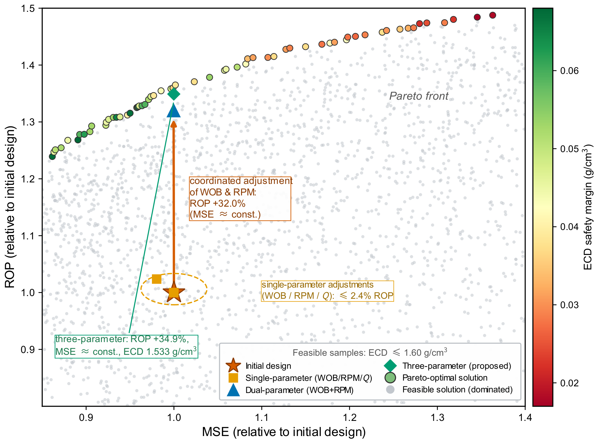
Operators can flexibly select the decision mode according to specific working conditions or manually pick suitable parameter combinations directly from the Pareto frontier.

3. Results and Discussion

3.1. Example Setup

To validate the effectiveness of the proposed method, numerical simulation examples are constructed. All data are generated from the hydraulic PDE numerical simulation described in Section 2, without involving laboratory or field experiments. The base well parameters are listed in

Table 3. Base well parameters.

Parameter	Value
Well depth	4000 m
Hole diameter	215.9 mm
Drill-pipe outer diameter	127 mm
Drill-collar outer diameter	158.8 mm
Drilling-fluid density	1.25 g/cm3
Cuttings density	2.65 g/cm3
Mean cuttings particle diameter	1.5 mm

. This includes the offset-well statistics: because no measured offset-well logs are available, the offset-well prior is prescribed rather than fitted—its mean comes from a regional depth trend and its covariance from an assumed inter-well variability, as specified in Section 2.6.2—and it is defined within the same synthetic parameter model that generates the observations, namely a regional depth trend plus a prescribed well-to-well offset, so that the ablation results reported below are fully reproducible from the code available from the authors.

The dynamic variations of the four parameters during drilling are simulated: $\mathrm{PV}$ and $\mathrm{YP}$ slowly decrease with increasing well depth due to rising temperature, $C_s$ varies with ROP fluctuations, and e increases with increasing well deviation. Gaussian noise with an amplitude of 5% is added to the observation data to simulate actual measurement errors. All inversion metrics are computed over $M=30$ independent noise realizations and reported as mean ± standard deviation.

The two priors of Section 2 are constructed as follows, and their mutual relation is stated explicitly because it determines how the inversion results of this section are to be interpreted. The offset-well prior is prescribed from a regional trend of the four parameters together with an assumed inter-well variability, the prior mean ${\mathit{\mu }}_{\mathrm{well}}$ being taken equal to that regional trend and the inter-well standard deviations being set to 6.0 mPa·s ($\mathrm{PV}$), 4.0 Pa ($\mathrm{YP}$), 0.02 ($C_s$) and 0.10 (e). The well under study is then offset from the regional trend by $\mathit{\delta }=(3.0\mathrm{mPa}·\mathrm{s},2.0\mathrm{Pa},0.01,0.04)$, which is smaller than one inter-well standard deviation on every parameter. The prior therefore contains no information about the well under study beyond the regional trend, and ${\mathit{\mu }}_{\mathrm{well}}$ does not coincide with the truth by construction: it differs from it by exactly $\mathit{\delta }$, so an inversion that is pinned to the prior mean is expected to inherit that difference rather than to remove it. The pre-drill baseline prior is set to the regionally averaged trend raised by 10%, representing the systematic offset of a pre-drill design. The consequences of this deliberate prior–truth mismatch are quantified in Section 3.2.4.

Three baseline methods are used for comparison: (i) traditional least-squares inversion (LS), which uses only pressure observations without prior constraints; (ii) a plain point-to-point MLP prediction model, which directly learns the input–output mapping without any physics residual term or explicit inversion module; and (iii) an online NSGA-II optimizer, which is a standard black-box evolutionary multi-objective algorithm run at the same sliding-window update frequency and under the same total surrogate-cost budget as the proposed method—using simulated binary crossover, polynomial mutation, non-dominated sorting and the constrained-domination principle—so that the comparison isolates the contribution of the surrogate and of the mechanism gradient, since NSGA-II exploits no gradient information. The budget is compared in terms of surrogate cost rather than of evaluation count, because the proposed method also spends backward passes; the accounting is defined in Section 3.4.3.

Three groups of evaluation metrics are adopted: (i) inversion accuracy, quantified by the root-mean-square error (RMSE) and mean absolute percentage error (MAPE) of each parameter; (ii) surrogate-model accuracy, quantified by the full-field relative $L_2$ error and inference time; and (iii) optimization performance, quantified by the ROP improvement rate, MSE reduction rate, safety margin, and a comprehensive efficiency index.

3.2. Analysis of Dual-Prior Constrained Inversion Results

3.2.1. Inversion Accuracy Comparison

Table 4. Comparison of inversion accuracy among different methods (mean ± std over 30 independent noise realizations).

Parameter	Method	RMSE	MAPE (%)
$\mathrm{PV}$ (mPa·s)	Least squares	$4.51\pm 0.44$	$10.95\pm 0.68$
	Baseline prior only	$3.93\pm 0.04$	$9.91\pm 0.14$
	Offset-well prior only	$2.97\pm 0.00$	$8.51\pm 0.00$
	Dual-prior (proposed)	$2.84\pm 0.00$	$8.06\pm 0.00$
$\mathrm{YP}$ (Pa)	Least squares	$1.64\pm 0.10$	$10.09\pm 0.58$
	Baseline prior only	$1.62\pm 0.03$	$9.44\pm 0.31$
	Offset-well prior only	$1.84\pm 0.01$	$13.87\pm 0.06$
	Dual-prior (proposed)	$1.72\pm 0.01$	$12.49\pm 0.05$
$C_s$	Least squares	$0.062\pm 0.002$	$81.53\pm 4.06$
	Baseline prior only	$0.004\pm 0.000$	$5.49\pm 0.06$
	Offset-well prior only	$0.010\pm 0.000$	$14.14\pm 0.01$
	Dual-prior (proposed)	$0.009\pm 0.000$	$13.31\pm 0.01$
e	Least squares	$0.262\pm 0.024$	$67.87\pm 8.56$
	Baseline prior only	$0.148\pm 0.000$	$42.57\pm 0.04$
	Offset-well prior only	$0.040\pm 0.000$	$12.26\pm 0.00$
	Dual-prior (proposed)	$0.040\pm 0.000$	$9.53\pm 0.00$

compares the estimation accuracy of the four parameters obtained by different inversion methods.

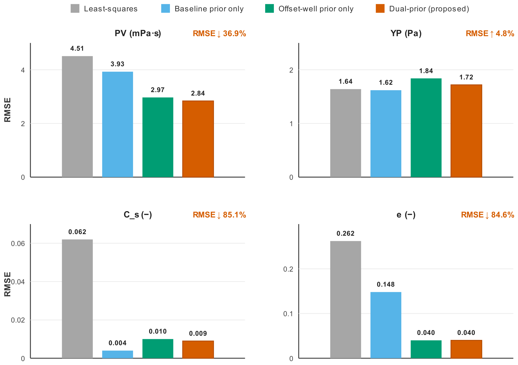
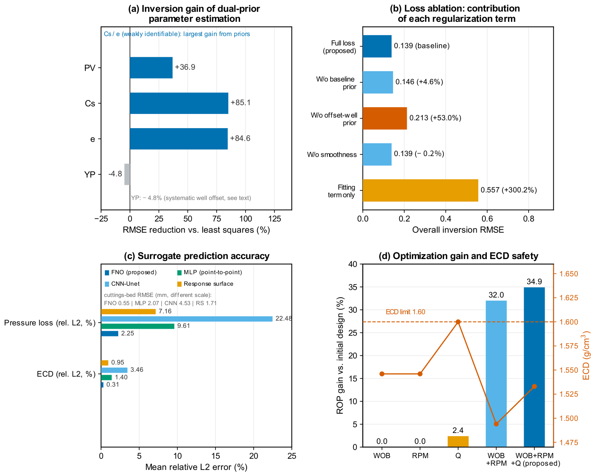
As can be seen from Table 4, the traditional least-squares inversion yields the largest errors, and the four parameters are improved to markedly different degrees by the priors, consistent with their distinct physical roles. The two weakly identifiable parameters—cuttings concentration $C_s$ and equivalent eccentricity e—benefit the most, with their RMSE reduced by 85.1% and 84.6%, respectively, because pressure and torque observations alone can hardly constrain them. Plastic viscosity $\mathrm{PV}$ is reduced by 36.9%. Yield point $\mathrm{YP}$ is essentially unchanged ($-4.8\%$), reflecting a small ($+2$ Pa) well-to-well offset of the current well relative to the regional trend that the offset-well prior does not capture; this is analyzed further in the prior-misspecification test below. Overall, the dual-prior mechanism provides a pronounced, parameter-specific regularization gain rather than a uniform one. Figure 2 summarizes this picture graphically for the plastic viscosity, whose absolute error is the largest of the four parameters: the RMSE falls monotonically from 4.51 mPa·s for least squares and 3.93 mPa·s for the baseline prior alone, to 2.97 mPa·s for the offset-well prior alone and 2.84 mPa·s for the dual prior.

3.2.2. Temporal Stability Analysis

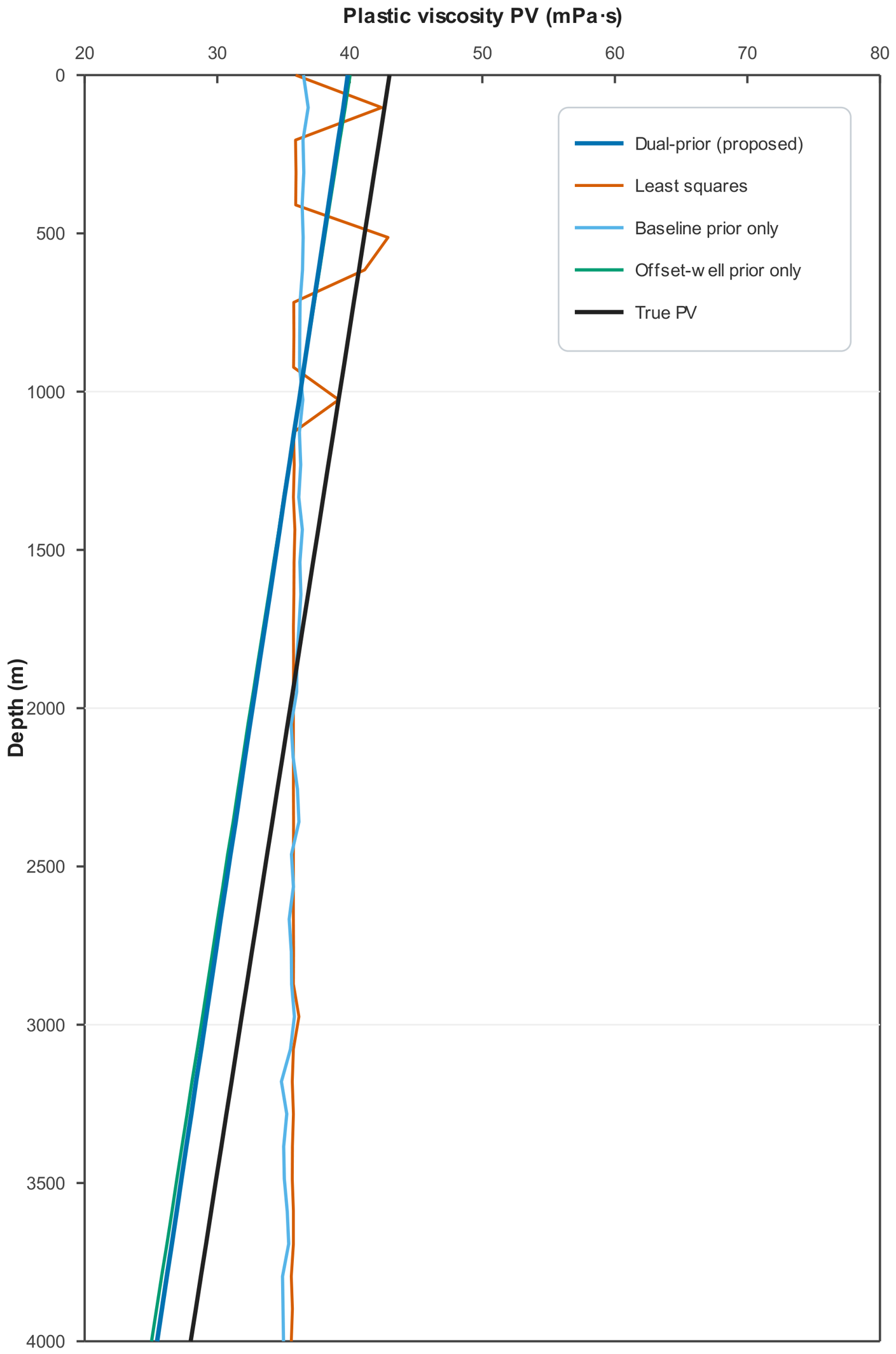
Figure 3 compares the plastic-viscosity estimates along the well depth. The least-squares inversion does not recover the depth trend at all. With two observations and four unknowns the fit term is rank-deficient, and the unregularized estimate remains essentially constant at the level of its starting point (35.75 mPa·s), departing from it only in a few noise-driven excursions. The dual-prior curve instead reproduces the trend over the whole interval and is temporally smooth, its random scatter being reduced from 4.00 to 0.17 mPa·s. A nearly constant offset nevertheless remains: the dual-prior estimate lies 2.84 mPa·s below the true $\mathrm{PV}$ curve, against 2.97 mPa·s for the offset-well prior alone. This residual is not a numerical artefact but the prescribed inter-well offset of ${\delta }_{\mathrm{PV}}=+3.0$ mPa·s between the current well and the regional trend. The offset-well prior is built from that regional trend and therefore carries no information about the level of the current well, while the level itself is not identifiable from the two observed channels and is inherited from the prior rather than determined by the data. What the priors contribute is the depth trend and the suppression of observation noise, not the absolute level; the same mechanism accounts for the unchanged $\mathrm{YP}$ RMSE in Table 4.

3.2.3. Ablation Experiments

To verify the independent contribution of each loss term, ablation experiments are designed, removing each term from the loss function one by one to compare the changes in inversion performance, as summarized in

Table 5. Ablation results of the loss function. The overall RMSE is the mean over the four parameters of ${\mathrm{RMSE}}_p/s_p$, with $s_p$ the characteristic scales of Section 2.6.3, so that it is dimensionless.

Loss Configuration	Overall RMSE	Relative Change
Full loss (proposed)	0.139	Baseline
Baseline regularization removed	0.146	+4.6%
Offset-well regularization removed	0.213	+53.0%
Smoothness constraint removed	0.139	$-0.2$%
Fitting term only	0.557	+300.2%

.

The ablation results show that the offset-well prior contributes the most: removing it increases the overall RMSE by 53.0%. The baseline prior contributes a smaller but still positive gain ($+4.6\%$). The smoothness constraint contributes negligibly under these slowly varying conditions ($-0.2\%$), which is expected because its role is largely redundant with the two priors. When all constraints are removed, leaving only the fitting term, the overall RMSE increases by 300.2%, confirming that the priors are essential for regularizing an otherwise rank-deficient inverse problem. The configuration in which only the smoothness term is removed also provides the like-for-like baseline in which least squares is given the same two priors as the proposed model, so that the two contributions can be separated. Per parameter, it gives RMSE values of $2.858\pm 0.002$ mPa·s ($\mathrm{PV}$), $1.740\pm 0.006$ Pa ($\mathrm{YP}$), $0.009$ ($C_s$) and $0.039$ (e), against $2.844$, $1.721$, $0.009$ and $0.040$ for the full model: the temporal term changes the per-parameter RMSE by at most 1.1% ($\mathrm{YP}$), so the improvement over unregularized least squares originates almost entirely from the two priors, and the temporal term acts as a marginal stabilizer rather than as the source of the gain.

The weights of Equation (20) were set by the one-at-a-time sweep of

Table 6. Sensitivity of the inversion accuracy to the weights of the four-term loss of Equation (20). Each column varies one weight while the other two are held at $1.0$. The entries are the same overall RMSE as in Table 5, i.e., the mean over the four parameters of ${\mathrm{RMSE}}_p/s_p$, reported as mean ± std over the $M=30$ noise realizations.

Weight Value	${\mathit{\lambda }}_1$ (Baseline)	${\mathit{\lambda }}_2$ (Offset-Well)	${\mathit{\lambda }}_3$ (Smoothness)
0	$0.1455\pm 0.0002$	$0.2129\pm 0.0009$	$0.1389\pm 0.0002$
0.1	$0.1446\pm 0.0002$	$0.1509\pm 0.0005$	$0.1389\pm 0.0002$
0.3	$0.1429\pm 0.0002$	$0.1362\pm 0.0004$	$0.1390\pm 0.0002$
1 (adopted)	$0.1392\pm 0.0002$	$0.1392\pm 0.0002$	$0.1392\pm 0.0002$
3	$0.1398\pm 0.0001$	$0.1452\pm 0.0001$	$0.1398\pm 0.0002$
10	$0.1602\pm 0.0001$	$0.1484\pm 0.0000$	$0.1421\pm 0.0002$

, in which each weight was varied over the range 0 to 10 while the other two were held at unity, all other settings being identical to Table 4.

Three features of the sweep support the adopted value ${\lambda }_i=1$. First, the minimum is a plateau rather than a point: ${\lambda }_1$ between $0.3$ and 3, and ${\lambda }_2$ between $0.3$ and 1, all lie within 3% of the best value, so the reported inversion accuracy does not depend on a finely tuned weight. Second, the response is asymmetric in a physically interpretable way. Over-weighting the baseline prior (${\lambda }_1=10$) raises the overall RMSE by 15% and doubles the eccentricity error, from $0.040$ to $0.081$, because the baseline prior then competes with the offset-well prior, which is the term that actually carries the depth trend; under-weighting the offset-well prior by a factor of ten (${\lambda }_2=0.1$) costs 8%, and switching it off costs 53%, consistent with Table 5. Third, ${\lambda }_3$ is essentially inert: between $0.1$ and 10 the overall RMSE varies by 2%, the cuttings-concentration error is unchanged at $0.009$, and only the eccentricity error moves appreciably, from $0.039$ to $0.050$. The standard deviations are negligible throughout, so the weights affect the bias of the estimate rather than its stability across noise realizations. The entries at $\lambda =0$ reproduce the corresponding rows of Table 5 to within rounding, which confirms that the two experiments measure the same quantity.

3.2.4. Robustness to Model-Form Error and Prior Misspecification

Both results reported above are obtained under an ideal condition that has to be examined explicitly. The observations are synthesized and inverted with the same forward operator, so the residual of the fitting term contains observation noise only and carries no model-form error; a favorable comparison under that condition does not by itself establish that the inversion survives a mismatch between the operator that generates the data and the operator used to invert them (an inverse crime).

To break this symmetry, a second and independently parametrized forward model was implemented. It differs from the inversion model in its rheological closure and in its constitutive corrections: an exponential eccentricity correction, a Thomas-type cuttings-friction relation, a modified annular shear-rate correction, and an explicit yield-dominated plug-flow pressure term. The test data were regenerated with this alternative closure while the inversion retained the original operator, and the comparison of Table 4 was repeated under otherwise identical settings; the outcome is reported in

Table 7. Inverse-crime test. RMSE (mean ± std over $M=30$ noise realizations) when the observations are generated by the same operator that is used in the inversion and when they are generated by the independently parametrized closure, the inversion operator being unchanged. All other settings are identical to Table 4.

	Least Squares		Dual-Prior (Proposed)
Parameter	Same Operator	Mismatched	Same Operator	Mismatched
$\mathrm{PV}$ (mPa·s)	$4.506\pm 0.443$	$4.495\pm 0.361$	$2.844\pm 0.002$	$2.843\pm 0.001$
$\mathrm{YP}$ (Pa)	$1.642\pm 0.098$	$1.737\pm 0.085$	$1.721\pm 0.006$	$1.716\pm 0.006$
$C_s$	$0.062\pm 0.002$	$0.059\pm 0.002$	$0.009\pm 0.000$	$0.009\pm 0.000$
e	$0.262\pm 0.024$	$0.240\pm 0.023$	$0.040\pm 0.000$	$0.040\pm 0.000$

.

The dual-prior errors are unchanged within the scatter over the 30 realizations (PV $2.844\to 2.843$ mPa·s, $\mathrm{YP}$ $1.721\to 1.716$ Pa, $C_s$ and e unchanged to the reported precision, i.e., a relative change of at most 0.3%), so the conclusions drawn from Table 4 are not an artifact of using one operator for both purposes. The least-squares errors move by up to 8% and not in a consistent direction ($\mathrm{PV}$ $4.506\to 4.495$, $\mathrm{YP}$ $1.642\to 1.737$, $C_s$ $0.062\to 0.059$, e $0.262\to 0.240$); this is expected, because the fitting term is rank-deficient (Section 3.2.5) and the unregularized estimate is governed by its starting point rather than by the forward operator, so the test is informative for the regularized estimator rather than for least squares.

The second test concerns the prior rather than the operator. The mean of the offset-well prior was displaced by one full inter-well standard deviation—6.0 mPa·s ($\mathrm{PV}$), 4.0 Pa ($\mathrm{YP}$), 0.02 ($C_s$) and 0.10 (e)—and the dual-prior inversion was rerun. Since the well under study lies within one inter-well standard deviation of the regional trend on every parameter (Section 3.1), this is a deliberately adversarial perturbation of the prior;

Table 8. Prior-misspecification test. RMSE (mean ± std over $M=30$ noise realizations) of the dual-prior inversion with the offset-well prior mean as prescribed and with the mean displaced by one standard deviation of ${\mathbf{\Sigma }}_{\mathrm{well}}$.

Parameter	${\mathit{\mu }}_{\mathbf{well}}$ as Prescribed	${\mathit{\mu }}_{\mathbf{well}}$ Displaced by $+1\mathit{\sigma }$
$\mathrm{PV}$ (mPa·s)	$2.844\pm 0.002$	$2.887\pm 0.002$
$\mathrm{YP}$ (Pa)	$1.721\pm 0.006$	$1.500\pm 0.013$
$C_s$	$0.009\pm 0.000$	$0.008\pm 0.000$
e	$0.040\pm 0.000$	$0.054\pm 0.000$

reports the result.

The estimate remains bounded and of the same order on every parameter ($\mathrm{PV}$ $2.844\to 2.887$ mPa·s, a change of 1.5%; $C_s$ $0.009\to 0.008$; e $0.040\to 0.054$, the largest degradation), so a prior error of one inter-well standard deviation perturbs the estimates without destabilizing the inversion. $\mathrm{YP}$ is the instructive case: its RMSE improves from $1.721$ to $1.500$ Pa, because the true $\mathrm{YP}$ of the well under study lies 2 Pa above the regional trend, an offset that is within the 4.0 Pa inter-well standard deviation, so a prior displaced upward by one standard deviation happens to move closer to the truth. This confirms that the mild degradation of $\mathrm{YP}$ in Table 4 is a genuine well-to-well offset rather than an inversion artifact. It also shows the limit of the test: the response is strongly parameter-specific, so the outcome cannot be summarized by a single number, and only the worst case for each parameter is meaningful.

3.2.5. Identifiability of the Fitting Term and the Covariance of the Estimate

The covariance of Equation (23) is the inverse of the Hessian of the total loss and therefore describes the regularized posterior, not the uncertainty implied by the observations alone. Since this covariance feeds the probabilistic safety constraints and thus the margins reported in Section 3.4.4, it is necessary to establish how much of the confidence interval originates from the data and how much from the priors. The two contributions can be separated by forming the Gauss–Newton approximation of the fitting-term Fisher information,

$${\mathit{H}}_{\mathrm{fit}}={\mathit{J}}^T\mathit{W}\mathit{J},$$

(42)

where $\mathit{J}$ is the $2\times 4$ Jacobian of the standpipe pressure and the rotary torque with respect to the four parameters and $\mathit{W}$ is the observation weighting of the fitting term. Evaluated at the optimum of the mid-depth window, ${\mathit{H}}_{\mathrm{fit}}$ has rank 2 while the parameter dimension is 4: the two observations span a two-dimensional subspace of the four-dimensional parameter space at most, so the fitting term is rank-deficient and its covariance matrix is singular, being defined only through a pseudo-inverse.

Table 9. Covariance of the estimate at the mid-depth window: standard deviations obtained from the Hessian of the total loss, as used in the safety constraints, and from the fitting term alone. Caution is needed in reading the second column, because the corresponding information matrix is rank-deficient (rank 2 of 4) and the pseudo-inverse distributes the variance among the parameters arbitrarily.

Parameter	Total Loss (Used in Section 3.4.4)	Fitting Term Only (Pseudo-Inverse)
$\mathrm{PV}$ (mPa·s)	4.1590	0.1650
$\mathrm{YP}$ (Pa)	2.5863	0.6407
$C_s$	0.0134	0.6655
e	0.0671	7.3690

reports the two covariances side by side.

The two covariances are not related by a scalar factor, and the split of the uncertainty among the parameters is not determined by the measurements. For $\mathrm{PV}$ and $\mathrm{YP}$ the fitting-term pseudo-inverse yields smaller standard deviations ($0.165$ against $4.159$ mPa·s and $0.641$ against $2.586$ Pa), whereas for the two weakly identifiable parameters, it yields much larger ones ($C_s$ $0.666$ against $0.013$, e $7.37$ against $0.067$). A pseudo-inverse of a rank-deficient information matrix distributes variance arbitrarily among the parameters and therefore cannot be read as a confidence interval; the regularized posterior is finite only because of the two priors. Since ${\mathit{H}}_{\mathrm{fit}}$ of Equation (42) has rank 2, the two observations determine at most two combinations of the four parameters, and the remaining directions are fixed by the priors alone; the tightness of the safety margins of Section 3.4.4 therefore derives from the prior assumptions rather than from the observations, and the reported margins should be interpreted as conditional on the priors being reasonably calibrated—which is what the sensitivity test of Section 3.2.4 probes. This is consistent with the loss ablation of Section 3, where retaining the fitting term alone degrades the overall RMSE from $0.139$ to $0.557$.

3.3. Performance Analysis of FNO Surrogate Model

3.3.1. Prediction Accuracy

Table 10. Comparison of surrogate-model prediction accuracy on the test set. ECD and pressure loss are reported as mean relative $L_2$ error; cuttings-bed height, a sparse quantity with near-zero mean, is reported as absolute RMSE. All four models are trained on the same 1200 samples and evaluated on the same 300-sample test set, the FNO being evaluated at $n_z=64$.

Method	ECD (%)	Pressure Loss (%)	Cuttings Bed RMSE (mm)
FNO (proposed)	0.31	2.25	0.55
MLP (point-to-point)	1.40	9.61	2.07
CNN-Unet (1D CNN)	3.46	22.48	4.53
Response surface	0.95	7.16	1.71

compares the prediction accuracy of the FNO surrogate model and other methods on the test set.

The proposed FNO is the most accurate of the four surrogates on all three outputs: 0.31% against 0.95% for the ECD, 2.25% against 7.16% for the pressure loss, and 0.55 mm against 1.71 mm for the cuttings-bed height. The strongest baseline is here the quadratic response surface rather than either neural baseline: the training labels are smooth, noise-free functions of the eight input parameters, and a closed-form least-squares fit of a quadratic polynomial in those parameters to the 192 output values is therefore a strong competitor, ahead of the point-to-point MLP (1.40%, 9.61%, 2.07 mm) and of the CNN (3.46%, 22.48%, 4.53 mm). A bootstrap over 1000 resamples of the test set shows that the ranking is resolved at the $1\sigma$ level on every channel ($0.31\pm 0.02$% against $0.95\pm 0.06$% for the ECD, $2.24\pm 0.20$% against $7.15\pm 0.40$% for the pressure loss, and $0.55\pm 0.02$ mm against $1.71\pm 0.08$ mm for the cuttings bed), so the advantage over the best baseline is statistically significant rather than marginal. The margin is about a factor of three on the ECD, a factor of 3.2 on the pressure loss and a factor of 3.1 on the cuttings bed, while the errors of the MLP and the CNN are three to ten times larger than those of the FNO. The gain over the point-to-point baselines is largest for the two fields that vary along the well depth: the MLP maps the input parameters to a fixed output vector and can only reproduce the depth profile through its fully connected weights, whereas the Fourier layers of the FNO act directly on the depth coordinate. A direct measure of this is the mean absolute deviation of each field from its depth average (normalized units, $n_z=64$): on the ECD, it is $2.24\times {10}^{-2}$ in the reference data, and the FNO and the quadratic response surface reproduce it to within 0.1%, whereas the MLP overshoots it to $2.48\times {10}^{-2}$, and the CNN recovers only $2.4\times {10}^{-3}$, about one tenth of the depth variation actually present in the reference field. The same ordering holds for the pressure loss and the cuttings-bed height. The response surface, which regresses every depth node separately, captures that profile and is accordingly the strongest of the three baselines, but it remains a factor of three behind the FNO and, being a fixed polynomial map, it has no notion of the depth grid.

3.3.2. Computational Efficiency

Table 11. Comparison of single-sample inference time. The reference simulation and the four surrogates are timed in the same process on the same workstation with an identical protocol (20 warm-up runs, then the median of 200 timed repetitions); the five models are measured in interleaved rounds and the reported value is the median over five such rounds, so every model is timed under the same machine state.

Method	Single-Sample Inference Time	Relative Speed-Up
Numerical simulation ($n_z=1024$)	125 ms	1×
FNO (proposed, $n_z=64$)	0.52 ms	240×
CNN-Unet ($n_z=64$)	0.11 ms	1140×
Response surface	0.046 ms	2720×
MLP (point-to-point)	0.012 ms	10,400×

compares the single-sample inference time of the four surrogates and of the reference numerical simulation, and Figure 4 shows the same comparison on a logarithmic scale.

The single-sample inference time of the FNO is 0.52 ms, about 240× faster than the reference numerical simulation at $n_z=1024$, which is what makes the hundreds of forward evaluations of the online loop affordable. The speed-up is, however, not the largest among the surrogates considered: the point-to-point MLP needs only 0.012 ms, the response surface 0.046 ms and the CNN 0.11 ms, so that in the present NumPy implementation the FNO is the slowest of the four. Its per-sample cost is dominated by the small-size FFTs and complex multiplications of the Fourier layers, which benefit only weakly from batching, whereas the dense matrix products of the MLP and of the response surface scale almost linearly with batch size; this is the price paid for the discretization invariance of Section 3.3.3, which the other three do not have. The FNO cost is also roughly independent of the depth-grid resolution, so the gap against the direct solver grows at finer grids. We note that the reference here is a semi-analytical one-dimensional model; against a fully three-dimensional solver, the advantage would be much larger, but the exact factor depends on the solver implementation.

3.3.3. Generalization Capability Test

Two tests are carried out on the trained surrogate: a 10% parameter extrapolation outside the training box, and a change of the depth-grid resolution at fixed weights. A third study isolates the effect of the physics-residual term added to the training loss.

Under the 10% parameter extrapolation, the FNO error grows only moderately, from 0.31% to 0.62% for the ECD, from 2.25% to 4.73% for the pressure loss, and from 5.81% to 11.66% for the cuttings bed, and it remains the most accurate of the four models: the quadratic response surface reaches 1.16%, 8.89% and 24.47%, the point-to-point MLP 1.88%, 13.57% and 29.68%, and the CNN 4.01%, 27.69% and 55.32%. Averaged over five independent extrapolation sets of 200 samples each, the FNO attains $0.87\pm 0.26$% and $7.94\pm 3.37$% on the ECD and the pressure loss against $2.06\pm 0.19$% and $15.60\pm 1.74$% for the MLP, and $16.39\pm 4.15$% against $35.72\pm 4.67$% for the cuttings bed, so that every gap is larger than the combined seed-to-seed scatter. It should be noted, however, that the operator form does not confer a qualitative extrapolation advantage: the absolute margin of the FNO over the MLP widens only slightly on the pressure loss (from 7.4 to 8.8 percentage points), while the relative margin narrows from a factor of 4.3 to 2.9. The defensible statement is that the FNO extrapolates as well as, and in absolute terms slightly better than, a well-tuned point-to-point baseline, and it is clearly better than the CNN and the response surface, rather than that it extrapolates fundamentally better.

The property that does distinguish the FNO is its discretization invariance. Because the operator is parameterized in Fourier space and the depth coordinate is supplied as an input channel, the same set of weights can be evaluated on a different number of depth nodes without retraining. Evaluated at 32, 64 and 128 nodes, the relative $L_2$ error of the single FNO model changes only from 2.43% to 2.25% and 2.27% for the pressure loss, and from 5.98% to 5.81% and 5.84% for the cuttings-bed field, i.e., by less than 0.2 percentage points over a fourfold change of the grid. The ECD is the exception: its error rises from 0.31% at the training resolution to 2.16% at 32 nodes and 1.35% at 128 nodes. Most of that increase is not a model error, because the reference ECD field is itself grid-dependent—its accumulation is normalized by the depth of the first node, which changes with $n_z$—and directly interpolating the $n_z=64$ reference solution onto the new grid already changes the ECD by 1.27% and 1.05%, respectively. The residual degradation attributable to the surrogate is therefore about 0.9 percentage points at 32 nodes and 0.3 of a point at 128 nodes. The other two reference fields are exactly grid-independent, since the coupled fixed point is solved independently at every node; they are reproduced by the single set of weights over the fourfold grid change without measurable loss. The MLP, CNN and response-surface baselines have a fixed output dimension tied to the training grid and cannot be evaluated on another grid at all; predicting on another grid requires retraining them. This resolution-independent operator representation, together with the accuracy of Table 10, is the reason for adopting the FNO in the online loop.

3.3.4. Physics-Residual Ablation

The training loss was extended with the two soft closure residuals of $\mathcal{H}$ and $\mathcal{E}$ described in the previous section.

Table 12. Effect of the physics-residual weight $\lambda$ on the FNO accuracy, under an identical training budget (250 epochs, mini-batch 256, $1200/300$ split). Errors are mean relative $L_2$ over the 300-sample test set; extrapolation is over five independent sets of 200 samples drawn from the range extended by 10% on each side.

	In-Domain Rel. ${\mathit{L}}_2$ (%)			10% Extrapolation (%)		5-Seed Extrapolation (%)
$\mathit{\lambda }$	${\mathbf{\partial }}_{\mathit{z}}\mathit{P}$	ECD	${\mathit{h}}_{\mathit{b}}$	${\mathbf{\partial }}_{\mathit{z}}\mathit{P}$	ECD	${\mathbf{\partial }}_{\mathit{z}}\mathit{P}$	ECD
0 (adopted)	2.25	0.31	5.81	4.73	0.62	$7.94\pm 3.37$	$0.87\pm 0.26$
${10}^{-3}$	2.49	0.48	6.48	5.07	0.71	$8.55\pm 3.46$	$0.90\pm 0.20$
${10}^{-2}$	3.77	0.76	9.80	6.97	1.05	$10.12\pm 2.64$	$1.26\pm 0.19$

reports the effect of their weight $\lambda$ under an otherwise identical training budget (same random seed, data split, batch size and learning-rate schedule).

The data do not support the physics-residual term. Accuracy degrades monotonically with $\lambda$ on every reported quantity—the pressure loss, the ECD and the cuttings-bed field, in-domain, under 10% extrapolation and across the five extrapolation seeds—so that the best configuration is the one in which the term is switched off. We note that the earlier version of this table contained a single reversal on the cuttings-bed error under 10% extrapolation; with the retrained surrogate of Table 10, that reversal disappears, and the ordering is monotonic throughout. The reason is visible in Table 2: the reference data satisfy all three closure relations, the momentum and ECD relations identically and the cuttings-bed relation to machine precision, so the residual is zero on every training label. A residual that is identically zero on the labels carries no information about the target that the data term does not already contain, and the only latitude it leaves the optimizer is to reshape the loss landscape, which in this case is harmful. The physical content of the problem is not lost by this: it is imposed one level up, in the generation of the labels, which are obtained by solving the coupled momentum–bed system to its converged fixed point.

It should be emphasized that the accuracy reported in Table 10 is not a product of the physics term: the configuration that attains it is trained with $\lambda =0$, and every non-zero weight tested makes it worse. The physics-informed loss is reported here as a tested and rejected design option, and the production surrogate is trained with $\lambda =0$.

3.4. Analysis of Multi-Objective Coordinated Optimization Results

3.4.1. Pareto Frontier Analysis

Figure 5 shows the resulting front in the ROP–MSE plane, colored by the remaining ECD safety margin. The front is extracted from 60,000 operating points sampled over the decision space (WOB $\in [50,300]$ kN, RPM $\in [40,180]$ rev/min, $Q\in [15,40]$ L/s) under the ECD safety constraint. The initial design lies strictly below the front, confirming that a substantial optimization margin is available. The front is markedly asymmetric: moving from the initial design to the front raises ROP by about 36% at essentially unchanged MSE, whereas the additional ROP available further along the front is marginal—raising MSE by 10% above the initial design buys only about 4% of additional ROP. The colouring shows that this residual gain is bought under a progressively tighter safety budget: the remaining ECD margin of the non-dominated points decreases along the front from about 0.068 g/cm³ near the initial design to about 0.017 g/cm³ at its high-ROP end, i.e., below the propagated ECD uncertainty of about 0.03 g/cm³ for roughly the last fifth of the front, so that the residual ROP at that end is bought without a safety margin that can be certified. The trade-off is therefore threefold, pitting drilling efficiency simultaneously against energy consumption and against the ECD safety margin.

3.4.2. Comparison of Different Optimization Strategies

Table 13. Performance comparison of different optimization strategies.

Optimization Strategy	ROP Gain (%)	MSE Red. (%)	ECD (g/cm3)	Eff. Index
Single-parameter (WOB)	0.0	0.0	1.546	1.00
Single-parameter (RPM)	0.0	0.0	1.546	1.00
Single-parameter (Q)	2.4	2.0	1.600	1.02
Dual-parameter (WOB + RPM)	32.0	0.0	1.494	1.32
Three-parameter (proposed)	34.9	0.0	1.533	1.35

compares the comprehensive performance of different optimization strategies.

Single-parameter optimization of WOB or RPM yields no improvement because the MSE constraint prevents raising either variable in isolation. The flow rate is the only decision variable that also raises the ECD, and increasing it alone returns a modest 2.4% ROP gain with a 2.0% MSE reduction but consumes the whole safety margin, the solution being pushed onto the 1.60 g/cm³ limit. Dual-parameter (WOB + RPM) optimization achieves a 32.0% ROP gain by jointly lowering WOB and raising RPM at unchanged MSE; this also lowers the ECD from 1.546 to 1.494 g/cm³ because a higher rotary speed reduces the effective annular viscosity, so the dual-parameter solution not only is safer than the single-parameter flow-rate one but also leaves the largest ECD margin of the table (0.106 g/cm³). The three-parameter coordinated optimization raises the gain further to 34.9% through the flow-rate degree of freedom, still at unchanged MSE and with the ECD 0.067 g/cm³ below the limit, yielding the best comprehensive efficiency index (1.35).

3.4.3. Comparison with an Online Black-Box Optimizer at Equal Surrogate Cost

The strategies of Table 13 differ in the number of decision variables, not in the optimizer, and none of them establish that the proposed online Bayesian optimizer is the better search strategy. The comparison made here therefore holds the optimization problem fixed and varies only the search: the proposed online Bayesian optimizer, an online NSGA-II, and a model-free random search are run on the same 40 sliding windows, on the same inverted parameter trajectory ${\mathit{\theta }}_k$, over the same decision variables and the same constraints.

The budget has to be defined with care because the three methods do not consume the same resource. NSGA-II and the random search evaluate only the forward surrogate, so their cost is the number of ECD evaluations. The proposed optimizer additionally propagates gradients backward through the FNO whenever it applies the mechanism-gradient refinement of Section 2, and a budget counted in forward evaluations alone would silently credit it with work that a black-box method cannot buy. Throughout this comparison the budget is therefore expressed as a surrogate cost, in which one forward evaluation counts as 1 and one backward pass counts as 2; the weight 2 is a conservative upper bound on the backward-to-forward cost ratio measured for this implementation on the workstation used here, which is of order unity (0.97–1.34 across repeated measurements), so the accounting is biased against the proposed method rather than in its favor. The feasibility-aware projection of the initial design and the projection of every refined candidate point are charged at the same rate. All three methods are stopped once the same total cost of 900 has been spent, which buys the proposed method 196 distinct surrogate evaluations, NSGA-II 880 evaluations (22 generations of 40 individuals), and the random search 900 evaluations.

Table 14. Comparison of three online optimizers on the same 40 sliding windows and under the same surrogate cost of 900 (one forward evaluation of the FNO counts as 1, one backward pass as 2, a conservative upper bound on the measured ratio, which is of order unity (0.97–1.34); every projection is charged). The ECD margin is the average distance of the recommended operating points from the 1.60 g/cm³ limit. The last column gives the number of distinct surrogate evaluations bought by the budget.

Optimizer	Mean ROP Gain (%)	Std	Min (%)	Max (%)	ECD Margin	FNO Evaluations
Online Bayesian (proposed)	32.42	3.44	24.03	36.59	0.026	196
Online NSGA-II	31.94	4.47	19.64	36.64	0.032	880
Random search (no model)	29.40	3.66	19.57	36.01	0.032	900

summarizes the outcome.

Three conclusions follow. First, the proposed optimizer attains the highest mean gain, 32.42% against 31.94% for NSGA-II and 29.40% for the model-free reference, and it does so with 4.5 times fewer distinct surrogate evaluations. The mechanism gradient is what makes that possible: because it drives each candidate onto the ECD boundary, where the constrained optimum lies, the budget is not spent on the interior of the feasible region. The same effect is visible in the recommended operating points themselves, which sit on average 0.026 g/cm³ from the ECD limit against 0.032 g/cm³ for both black-box references—the surrogate-guided search pushes against the constraint while the two references stop short of it—and every one of the 40 windows returned a feasible recommendation in all three methods. Second, the margin over NSGA-II is not resolved by this experiment. The paired per-window difference is $+0.48$ percentage points (paired standard deviation 3.6, $t=0.83$, bootstrap 95% confidence interval $[-0.59,+1.62]$), and the two methods win 20 of the 40 windows each; only the difference against the model-free reference is resolved, $+3.01$ points (95% confidence interval $[+1.93,+4.04]$), with the proposed method ahead in 33 of 40 windows. Third, the two leading methods differ in their failure modes rather than in their average: the worst window of the proposed optimizer gains 24.03%, against 19.64% for NSGA-II and 19.57% for the random search, and its spread is the smallest of the three (3.44 against 4.47 and 3.66). The advantage is moreover concentrated where the problem is hardest—over the first 16 windows, in which the feasible fraction of the operating box is smallest, the proposed method leads NSGA-II by 2.1 points on average, whereas over the last 24 windows, once the feasible region has widened, it trails by 0.6 points.

The comparison above is made at a single budget, but the three strategies also differ in how fast they reach a given gain.

Table 15. Mean ROP gain (%) over the 40 sliding windows as a function of the surrogate cost already spent, for the three optimizers of Table 14. The curve of the proposed method starts at a cost of about 280, which is the price of its feasibility-aware initial design; dashes indicate that no operating point has been evaluated yet at that cost. The entries are read off the running experiment once the stated amount of cost has been spent: the proposed method stops at a mean cost of 904, so its 900 entry (32.30%) is not its final value, and the final mean gain of the completed run (32.42%) is the one listed in Table 14.

Surrogate Cost	200	300	400	500	600	700	800	900
Online Bayesian (proposed)	—	$-2.27$	25.25	29.48	31.22	31.56	32.09	32.30
Online NSGA-II	21.00	22.79	25.96	27.38	29.13	29.99	31.08	31.94
Random search (no model)	25.81	27.53	27.91	28.26	28.58	28.70	29.30	29.40

therefore reports the mean gain that each method has attained by the time a given amount of surrogate cost has been spent, i.e., the anytime behavior of the same 40-window experiment.

Judged by the cost of a given gain, the proposed method reaches the level that NSGA-II attains at a cost of 900 (31.94%) at a cost of about 770, a 1.17-fold saving, whereas the model-free reference does not reach that level within the budget at all. It overtakes both black-box references at a cost of about 400 and stays ahead of them at every larger budget. The price is paid at the small-budget end, and it is substantial: the feasibility-aware initialization and the projections that make the candidate points satisfy the ECD constraint consume about 280 of the 900 units before the first informative evaluation, so that at a cost of 300 the proposed method is 25 points behind the black-box references. Below a cost of roughly 400 a plain evolutionary or even a random search is therefore the better choice; the advantage of the FNO gradients appears only once a window can afford a few hundred surrogate evaluations, which is the regime of the present application.

3.4.4. Effect of Probabilistic Safety Constraints

The probabilistic safety constraint is imposed on the upper confidence bound of the ECD rather than on its mean value, so that the optimizer must reserve room for the posterior uncertainty of the inverted parameters. This distinction matters because the ECD inherits that uncertainty: propagating the dual-prior posterior standard deviations of Table 4 through the forward model gives an ECD standard deviation of the order of 0.03 g/cm³ at the baseline flow rate, and the variance is dominated by the annular cuttings concentration $C_s$, with secondary contributions from the yield point and the plastic viscosity and a negligible contribution from the equivalent eccentricity. A constraint on the mean ECD alone would therefore admit operating points whose true ECD exceeds 1.60 g/cm³ as soon as $C_s$ is over-estimated, whereas constraining the confidence bound forces the solution back into the interior of the feasible region. Consistently, the two strategies that dispose of the WOB and RPM degrees of freedom—the dual- and the three-parameter solutions of Table 13—retain an ECD margin of 0.106 and 0.067 g/cm³, i.e., two to three times the propagated ECD uncertainty of about 0.03 g/cm³. The single-parameter flow-rate solution is the one exception and reaches the limit exactly: with a single degree of freedom, there is no other variable left to trade the consumed ECD against, which is precisely the situation the constraint is meant to expose. One qualification follows from the identifiability analysis of Section 3.2.5: because the fitting term is rank-deficient, the width of these confidence intervals—and hence the amount of ECD margin that the constraint enforces—is set by the prior assumptions rather than by the observations. The margins reported here should therefore be read as conditional on the two priors being reasonably calibrated, and the sensitivity of the inversion to a prior error of one inter-well standard deviation is quantified in Section 3.2.4.

3.4.5. Re-Evaluation of the Recommended Operating Points with the Forward Solver

The operating points of Table 13 are recommended by the FNO surrogate, and the safety margin reported for them is the margin predicted by that surrogate. The two objective functions are evaluated from their closed-form expressions and are therefore unaffected by surrogate error, so the ECD constraint is the only quantity that requires independent verification. Each recommended operating point was consequently returned to the reference forward solver of Section 2 at $n_z=64$, and the resulting ECD and remaining margin are compared in

Table 16. Re-evaluation of the recommended operating points with the reference forward solver instead of the FNO surrogate. The deviation is defined as ECD_FNO–ECD_solver; the margins are measured from the 1.60 g/cm³ limit. The two objective functions are analytic and are not affected by the surrogate.

Operating Point	ECD (FNO)	ECD (Solver)	Deviation	Margin (FNO)	Margin (Solver)
Single-parameter (WOB)	1.5456	1.5427	$+0.0029$	0.0544	0.0573
Single-parameter (RPM)	1.5457	1.5428	$+0.0029$	0.0543	0.0572
Single-parameter (Q)	1.6000	1.6176	$-0.0176$	0.0000	$-0.0176$
Dual-parameter (WOB + RPM)	1.4943	1.4932	$+0.0011$	0.1057	0.1068
Three-parameter (proposed)	1.5334	1.5295	$+0.0039$	0.0666	0.0705

with the values the optimizer used.

At four of the five operating points, the surrogate and the solver agree to within 0.004 g/cm³, that is, within 0.3% of the nominal ECD and of the same order as the 0.31% test-set error of Table 10; in each of those four cases, the surrogate ECD is the higher of the two, so the margin reported by the optimizer is conservative by at most that amount. The single-parameter flow-rate point is a genuine exception, and an instructive one. The surrogate returns exactly the limiting value, 1.6000 g/cm³, whereas the solver returns 1.6176 g/cm³: the surrogate underestimates the ECD by 0.0176 g/cm³, and the recommended point therefore exceeds the safety limit by that amount instead of sitting on it. The reason is structural rather than accidental. With a single decision variable, there is nothing left to trade the consumed ECD against, so the solution is driven onto the constraint surface and its remaining margin is zero by construction; but a margin of zero lies inside the error bar of any surrogate whose ECD error is 0.3% of 1.60 g/cm³, i.e., about 0.005 g/cm³, and cannot be certified at that accuracy. The dual- and three-parameter recommendations are in a different position: their solver margins are 0.107 and 0.071 g/cm³, two to three times the 0.03 g/cm³ ECD uncertainty propagated from the inversion, and one to two orders of magnitude above the 0.001 and 0.004 g/cm³ by which the surrogate is optimistic at those two points, so they remain feasible when re-evaluated with the solver. The practical conclusion is that a surrogate-based recommendation should be required to retain a residual margin rather than to touch the limit, and that the number of decision degrees of freedom determines whether such a margin is available at all: the single-parameter solution consumes it entirely. This is also the quantitative justification for the design choice of Section 3.4.4, where the probabilistic constraint is imposed on the upper confidence bound of the ECD rather than on its mean, which holds the solution off the limit by the very amount measured here.

3.5. Ablation Experiment Analysis

To verify the contribution of each core module, the ablation study examines four aspects of the framework independently: the inversion accuracy gain brought by the dual-prior constraint relative to unconstrained least squares (Table 4), the contribution of each regularization term of the loss function (Table 5), the prediction accuracy of the surrogate models (Table 10), and the optimization gain together with the ECD safety margin of the single-, dual- and three-parameter strategies (Table 13). Figure 6 collects these four aspects into a single plate.

Figure 6a reports the per-parameter RMSE reduction of the dual-prior inversion relative to least squares. The gain is strongly parameter-dependent: the two weakly identifiable parameters, the annular cuttings concentration and the equivalent eccentricity, improve by 85.1% and 84.6%, respectively, and the plastic viscosity improves by 36.9%. The yield point is the exception ($-4.8\%$) because its least-squares estimate is already close to the pre-drill baseline value, so anchoring the solution to that baseline brings no further benefit; the small degradation is a systematic well offset rather than a loss of identifiability. Figure 6b isolates the contribution of each loss term. Removing the offset-well prior raises the overall inversion RMSE from 0.139 to 0.213 ($+53.0\%$), by far the largest single degradation, whereas removing the temporal smoothness term leaves the RMSE unchanged (0.139, $-0.2\%$) because its regularizing effect is largely redundant with the two priors under slowly varying conditions. Retaining the fitting term alone is far worse (0.557, $+300.2\%$), which quantitatively confirms the rank deficiency of the dual-observation fitting problem and shows that the priors, not the measurements, are what bound the covariance of the estimate. Figure 6c compares the surrogate models: the proposed FNO is the most accurate of the four on every output (0.31% against 0.95% for the ECD, 2.25% against 7.16% for the pressure loss, and 0.55 mm against 1.71 mm for the cuttings bed, the reference being the quadratic response surface), and the bootstrap intervals of Table 10 resolve the ranking at the $1\sigma$ level on all three channels; the margin over that strongest baseline is about a factor of three, and the FNO additionally retains a resolution-independent operator representation, one set of weights reproducing its accuracy when the depth grid is changed, whereas the other surrogates must be retrained. Figure 6d couples the optimization gain with the safety margin: single-parameter adjustments of WOB or RPM leave the initial design unchanged and raising the flow rate alone returns only 2.4%, whereas the dual- and three-parameter strategies raise ROP by 32.0% and 34.9% at unchanged MSE, with the dual- and three-parameter operating points keeping an ECD of 1.494 and 1.533 g/cm³, strictly below the 1.60 g/cm³ limit.

Taken together, the four panels show that the three modules contribute along different axes and cannot substitute for one another. The dual-prior constraint is what makes the inversion well posed: it removes the rank deficiency of the fitting term and delivers the largest error reduction for the weakly identifiable parameters, with the offset-well prior as the dominant term. The FNO surrogate is what makes the online loop affordable and grid-independent: it is roughly 240× faster than the reference numerical simulation, it is the most accurate of the four surrogates on every output field, and its accuracy for the two phase-distribution fields is preserved when the depth grid is changed without retraining. The coordinated multi-parameter optimization is what converts the improved parameter estimates into an actual gain: any single-parameter adjustment is blocked by the MSE or the ECD constraint and yields at most 2.4% ROP, whereas the joint WOB–RPM–Q strategy reaches 34.9% while keeping an ECD of 1.533 g/cm³ inside the limit. Removing any one of the three modules therefore degrades a different aspect of the framework—accuracy, efficiency, or optimization gain—which is the quantitative basis for the three-layer design adopted in this study.

3.6. Discussion

3.6.1. Mechanistic Interpretation of the Inversion Improvement

The inversion accuracy gain originates from two coupled mechanisms. First, the dual observations resolve the ill-posedness inherent in single-channel inversion: standpipe pressure primarily constrains the frictional and hydraulic characteristics of the system, whereas rotary torque carries complementary information on the rheological and velocity-field state, so their joint fitting substantially improves parameter identifiability. Second, the two priors play complementary roles in stabilizing the solution. The pre-drill mechanistic baseline prior anchors the inverted parameters to the physically expected range, preventing convergence to non-physical solutions, while the offset-well statistical prior encodes block-scale correlations among parameters through the Mahalanobis distance, which suppresses the high-frequency fluctuations induced by observation noise. This explains the ablation results: removing the offset-well prior degrades the RMSE most severely (53.0%) because it carries the strongest statistical information, whereas the smoothness constraint contributes negligibly ($-0.2\%$) because its role is largely redundant with the two priors under slowly varying conditions.

3.6.2. Mechanistic Interpretation of the Surrogate Efficiency and Generalization

Three properties of the FNO need to be distinguished. The first is accuracy. By parameterizing the integral kernel directly in Fourier space, the FNO learns a mapping between function spaces rather than a discrete point-to-point mapping, and it is the most accurate of the four surrogates on every output field, both in-domain (0.31% against 0.95% for the ECD, 2.25% against 7.16% for the pressure loss and 0.55 against 1.71 mm for the cuttings bed) and under the 10% parameter extrapolation. One qualification is nevertheless necessary: the advantage is quantitative rather than qualitative. Outside the training range the absolute margin of the FNO over the point-to-point MLP widens only from 7.4 to 8.8 percentage points, while its relative margin narrows from a factor of 4.3 to 2.9, so the operator form improves the accuracy of the extrapolated field without altering the way the error grows beyond the training box. The second property is discretization invariance, and it is here that the operator representation earns its place. Because the kernel is parameterized in Fourier space and the depth coordinate is supplied as an input channel, the same weights can be evaluated on 32, 64 or 128 depth nodes: the pressure-loss and cuttings-bed errors change by less than 0.2 percentage points over a fourfold change of the grid, while the ECD error rises from 0.31% to between 1.35% and 2.16%, of which 1.0–1.3 percentage points are already present in the reference field itself, because the accumulation that defines the ECD is normalized by the depth of the first node and therefore changes with $n_z$. The MLP, CNN and response surface have a fixed output dimension tied to the training grid and must be retrained for any other grid. The third property is the one that did not survive the test. Adding two analytic closure relations of the forward model as soft physics residuals was expected to improve both accuracy and physical consistency, and instead accuracy degrades monotonically with the weight $\lambda$, the best configuration being the one in which the term is switched off. The reason is structural rather than numerical: once the forward model is solved to its converged coupled fixed point, all three closure relations are satisfied by the reference data to machine precision—the largest residual is $1.2\times {10}^{-13}$ m—so their residuals vanish on the labels and the penalty adds no information about the target. In this forward model, the output fields already lie on a lower-dimensional, exactly self-consistent manifold, and the useful inductive bias is the operator architecture rather than an additional physical penalty; the physical content of the closures is imposed one level up, in the generation of the training labels. The roughly 240-fold inference speed-up over the numerical simulation follows from a different source—a single feed-forward pass in place of an iterative solution of the coupled equations—and it is worth stating plainly that among the four surrogates the FNO is the slowest in the present implementation since its Fourier layers are less amenable to dense batching than the matrix products of the MLP; this is the price paid for the discretization invariance, which none of the other three offer.

3.6.3. Mechanistic Interpretation of the Coordinated Optimization Gain

The 34.9% rate-of-penetration improvement of three-parameter optimization over single-parameter optimization reflects the exploitation of the intrinsic hydraulic–mechanical coupling among WOB, RPM, and flow rate. WOB and RPM jointly govern the rock-breaking rate and hence the cuttings generation rate, while the flow rate governs the cuttings-carrying capacity and the annular pressure loss; adjusting WOB or RPM alone leaves the initial design unchanged, and raising the flow rate alone returns only 2.4% while consuming the entire ECD safety margin. The coordinated formulation explores the joint feasible region, and the probabilistic safety constraints additionally prevent the optimizer from recommending points whose true ECD may violate the safe window under inversion uncertainty, thereby achieving a robust balance among safety, efficiency, and energy consumption.

3.6.4. Limitations and Assumptions

The proposed method still has certain limitations. First, all experimental data in this study are generated by the in-house hydraulic PDE numerical simulation without validation against field measured data; although the simulated conditions cover most conventional drilling scenarios, they cannot fully replicate complex geological disturbances, instrument anomalies, and sudden drilling-fluid performance changes, so the field adaptability of the method still requires further engineering verification. In particular, because the surrogate labels and the test data are drawn from the same solver, the reported 0.31% ECD and 2.25% pressure-loss errors are a self-consistent upper bound on the field accuracy rather than field-level figures. Second, the inverted parameters only focus on rheological parameters, cuttings concentration, and equivalent eccentricity, without considering special downhole complex conditions such as gas influx, wellbore collapse, and lost circulation, which limits the applicability under abnormal working conditions. Third, the FNO surrogate is trained purely on data: solved to its converged coupled fixed point, the forward model satisfies all three of its closure relations to machine precision, so none of them can be imposed as a non-redundant training constraint, as the ablation of Section 3.3.4 shows. Physical constraints could not therefore be exploited in the present setting, and its accuracy still decays under extrapolation beyond the training range (the pressure-loss error grows from 2.25% to 7.94% and the ECD error from 0.31% to 0.87% over five independent extrapolation sets), and its inference cost remains higher than that of a simple multilayer perceptron. Fourth, the optimization decision mode relies on preset weighting and rule-based selection, without incorporating drilling-expert experience and real-time condition-aware intelligent decision-making, so the intelligence level can still be improved.

3.7. Future Works

To address the above limitations, future research can proceed along the following directions:

• Broader validation and engineering deployment. Collect field drilling data to fine-tune model parameters and constraint weights according to field working conditions, and complete engineering adaptation and deployment verification of the method across diverse geological basins.
• Extension of the inversion parameter dimensionality. Introduce variables such as gas-influx rate, lost-circulation volume, and wellbore-stability parameters to construct a multi-parameter intelligent inversion system for complex downhole conditions.
• Physics-enhanced surrogate modeling with informative constraints. In the present model, the three closure relations are satisfied by the labels to machine precision, so none of them carry information that the data do not already contain. A more promising route is to target a formulation in which the reduced closure relations hold only approximately—for example, a transient or multi-dimensional solver in which the steady one-dimensional balances are no longer exact—so that a residual with independent information becomes available and can be imposed together with the discretization invariance of the operator representation. Combining such a constraint with the operator form is the natural way to improve extrapolation accuracy and physical rationality simultaneously.
• Adaptive intelligent decision-making. Introduce reinforcement learning and expert systems to construct an adaptive intelligent decision-making mechanism, realizing fully automatic optimal parameter decisions under different formations and working conditions.

4. Conclusions

Aiming at the technical problems of low dynamic identification accuracy of hydraulic parameters, insufficient hydraulic-field prediction efficiency, isolated static optimization of drilling parameters, and the difficulty in balancing safety and efficiency during drilling in deep complex formations, this study proposes a WOB–RPM–flow-rate coordinated optimization method driven by dual-prior-constrained temporal inversion and an FNO surrogate model. A three-layer integrated while-drilling intelligent decision-making framework of “parameter inversion–hydraulic prediction–intelligent optimization” is constructed. The effectiveness of the method is verified through theoretical derivation and multiple groups of numerical simulation experiments. The main conclusions are summarized as follows:

• A dual-prior-constrained temporal inversion module is constructed, fusing the pre-drilling mechanism baseline prior and the offset-well statistical prior, combined with standpipe pressure–rotary torque dual-observation information and temporal smoothness constraints. A four-term weighted loss function is designed, effectively improving the ill-posedness of multi-parameter inversion. Compared with the traditional least-squares single-observation inversion method, the inversion RMSE is reduced by up to 85% for the weakly identifiable parameters (cuttings concentration and equivalent eccentricity) and by 37% for plastic viscosity, enabling accurate and stable identification of the dynamic variations of plastic viscosity, yield point, average annular cuttings concentration, and equivalent eccentricity, with excellent anti-noise performance and temporal stability.
• The Fourier neural operator is applied to eccentric rotating-annular two-phase-flow hydraulic prediction for the first time, and a one-dimensional FNO surrogate model adapted to the drilling-fluid hydraulics scenario is constructed, with the well-depth coordinate supplied as an input channel so that the network can represent the profile along the wellbore. The model maps drilling operational and rheological parameters to the full-field hydraulic response with a mean relative error of 0.31% for equivalent circulating density, 2.25% for pressure loss and 0.55 mm for the cuttings-bed height, about three times lower than the error of the best of the three baselines tested (a quadratic response surface, 0.95% and 7.16%) and preserving that lead outside the training range. Its distinctive property is discretization invariance: a single set of weights reproduces the accuracy of the two phase-distribution fields when the depth grid is changed from 32 to 128 nodes without retraining, which none of the baseline surrogates can do, the ECD being the one field whose error grows because its reference definition is itself grid-dependent. The inference time is about 240 times lower than that of the reference numerical simulation, providing efficient computational support for real-time online optimization, although it remains the highest among the four surrogates considered here. Two design choices underlying this accuracy were established through controlled experiment: enlarging the network to four Fourier layers with 48 hidden channels and 12 modes, and replacing full-batch training by 256-sample mini-batches over 250 epochs. Adding two analytic closure relations of the forward model as soft physics residuals did not improve accuracy and was rejected because the reference data satisfy all three closures to machine precision and the residuals therefore carry no information about the target.
• A hydraulic–mechanical coupled three-parameter multi-objective coordinated optimization framework is established, with drilling-efficiency maximization and energy-consumption and risk minimization as the core objectives. Combined with online Bayesian optimization, mechanism-gradient acceleration, and the sliding-window rolling update mechanism, dynamic coordinated optimization of WOB, RPM, and flow rate is realized. Probabilistic safety constraints based on the confidence intervals of inverted parameters effectively reduce optimization risks arising from parameter uncertainty. Compared with the single-parameter optimization schemes, the rate of penetration is improved by 34.9%, while the mechanical specific energy is held essentially constant and the equivalent circulating density remains 0.067 g/cm³ below its limit, achieving a balanced trade-off among drilling safety, efficiency, and energy consumption.
• Ablation experiments verify the independent value and coupling gain effect of each module in the three-layer framework: dual-prior constraints guarantee parameter-identification accuracy, the FNO surrogate model provides efficient forward-modeling support, and online probabilistic optimization achieves dynamic robust decision-making. The synergistic interaction of the three modules jointly constitutes the core advantage of the proposed method, which can provide a novel theoretical method and technical support for real-time intelligent regulation of safe and efficient drilling in deep and ultra-deep wells with narrow windows.

In the future, field drilling data can be combined to complete model engineering adaptation, the capability of identifying complex downhole abnormal working conditions can be expanded, model performance can be optimized by integrating physical constraints and intelligent algorithms, and the field deployment and application of drilling-fluid hydraulic intelligent inversion and parameter optimization technology can be further promoted.

References

1. Vajargah, A.K.; van Oort, E. Determination of drilling fluid rheology under downhole conditions by using real-time distributed pressure data. J. Nat. Gas Sci. Eng. 2015, 24, 400–411. [Google Scholar] [CrossRef] [Scilit]
2. He, M.; Chen, X.; Xu, M.; Chen, H. Inversion-based model for quantitative interpretation by a dual-measurement points in managed pressure drilling. Process Saf. Environ. Prot. 2022, 165, 969–976. [Google Scholar] [CrossRef] [Scilit]
3. Fu, J.; Liu, W.; Zheng, X.; Han, X. Transfer Forest: A Deep Forest Model Based on Transfer Learning for Early Drilling Kick Detection. Energies 2023, 16, 2100. [Google Scholar] [CrossRef] [Scilit]
4. Maksimov, D.; Pavlov, A.; Sangesland, S. Real-Time Detection of Karstification Hazards While Drilling in Carbonates. Energies 2022, 15, 4951. [Google Scholar] [CrossRef] [Scilit]
5. Kaasa, G.-O.; Stamnes, Ø.N.; Imsland, L.; Aamo, O.M. Simplified hydraulics model used for intelligent estimation of downhole pressure for a managed-pressure-drilling control system. SPE Drill. Complet. 2012, 27, 127–138. [Google Scholar] [CrossRef] [Scilit]
6. Hauge, E.; Aamo, O.M.; Godhavn, J.M. Model-based estimation and control of in/out-flux during drilling. In Proceedings of the 2012 American Control Conference (ACC), Montreal, QC, Canada, 27–29 June 2012; IEEE: Piscataway, NJ, USA, 2012; pp. 4909–4914. [Google Scholar] [CrossRef] [Scilit]
7. Altindal, M.C.; Rasheed, A.; Nybø, R. Online parameter calibration in drilling hydraulics model. In Proceedings of the SPE Gas & Oil Technology Showcase and Conference (GOTECH), Dubai, UAE, 21–23 April 2025; SPE-224509-MS; SPE: Richardson, TX, USA, 2025. [Google Scholar] [CrossRef] [Scilit]
8. Arévalo, P.J.; Forshaw, M.; Starostin, A.; Aragall, R.; Grymalyuk, S. Monitoring hole-cleaning during drilling operations: Case studies with a real-time transient model. In Proceedings of the SPE Annual Technical Conference and Exhibition, Houston, TX, USA, 3–5 October 2022; SPE-210244-MS; SPE: Richardson, TX, USA, 2022. [Google Scholar] [CrossRef] [Scilit]
9. Gomar, M.; Elahifar, B. Application of Digitalization in Real-Time Analysis of Drilling Dynamics Using Along-String Measurement (ASM) Data Along Wired Pipes. Energies 2022, 15, 8930. [Google Scholar] [CrossRef] [Scilit]
10. Han, Y.; Zhang, X.; Xu, Z.; Song, X.; Zhao, W.; Zhang, Q. Cuttings Bed Height Prediction in Microhole Horizontal Wells with Artificial Intelligence Models. Energies 2022, 15, 8389. [Google Scholar] [CrossRef] [Scilit]
11. Akhshik, S.; Behzad, M.; Rajabi, M. CFD–DEM approach to investigate the effect of drill pipe rotation on cuttings transport behavior. J. Pet. Sci. Eng. 2015, 127, 229–244. [Google Scholar] [CrossRef] [Scilit]
12. Zakeri, A.; Alizadeh Behjani, M.; Hassanpour, A. Fully Coupled CFD–DEM Simulation of Oil Well Hole Cleaning: Effect of Mud Hydrodynamics on Cuttings Transport. Processes 2024, 12, 784. [Google Scholar] [CrossRef] [Scilit]
13. Raissi, M.; Perdikaris, P.; Karniadakis, G.E. Physics-informed neural networks: A deep learning framework for solving forward and inverse problems involving nonlinear partial differential equations. J. Comput. Phys. 2019, 378, 686–707. [Google Scholar] [CrossRef] [Scilit]
14. Mao, Z.; Jagtap, A.D.; Karniadakis, G.E. Physics-informed neural networks for high-speed flows. Comput. Methods Appl. Mech. Eng. 2020, 360, 112789. [Google Scholar] [CrossRef] [Scilit]
15. Wu, L.; Zhang, Z.; Zhang, C.; Li, G.; Song, X.; Zhou, M.; Yao, X. Physics-Informed Fusion Neural Network for Real-Time Bottomhole Pressure Control in Managed Pressure Drilling. Processes 2026, 14, 1240. [Google Scholar] [CrossRef] [Scilit]
16. Li, Z.; Kovachki, N.; Azizzadenesheli, K.; Liu, B.; Bhattacharya, K.; Stuart, A.; Anandkumar, A. Fourier neural operator for parametric partial differential equations. In Proceedings of the International Conference on Learning Representations, Virtual Event, 3–7 May 2021. [Google Scholar]
17. Kovachki, N.; Li, Z.; Liu, B.; Azizzadenesheli, K.; Bhattacharya, K.; Stuart, A.; Anandkumar, A. Neural operator: Learning maps between function spaces with applications to PDEs. J. Mach. Learn. Res. 2023, 24, 1–26. [Google Scholar]
18. Guo, Q.; He, Y.; Liu, M.; Zhao, Y.; Liu, Y.; Luo, J. Reduced geostatistical approach with a Fourier neural operator surrogate model for inverse modeling of hydraulic tomography. Water Resour. Res. 2024, 60, e2023WR034939. [Google Scholar] [CrossRef] [Scilit]
19. Liu, Q.; Ni, F.; Hui, G. A machine learning-driven framework for real-time lithology identification and drilling parameter optimization. Processes 2026, 14, 156. [Google Scholar] [CrossRef] [Scilit]
20. Nystad, M.; Aadnøy, B.S.; Pavlov, A. Real-time minimization of mechanical specific energy with multivariable extremum seeking. Energies 2021, 14, 1298. [Google Scholar] [CrossRef] [Scilit]
21. Song, J.; Wang, J.; Li, B.; Gan, L.; Zhang, F.; Wang, X.; Wu, Q. Real-time drilling parameter optimization model based on the constrained Bayesian method. Energies 2022, 15, 8030. [Google Scholar] [CrossRef] [Scilit]
22. Boukredera, F.S.; Youcefi, M.R.; Hadjadj, A.; Ezenkwu, C.P.; Vaziri, V.; Aphale, S.S. Enhancing the drilling efficiency through the application of machine learning and optimization algorithm. Eng. Appl. Artif. Intell. 2023, 126, 107035. [Google Scholar] [CrossRef] [Scilit]
23. Kim, J.; Cho, M.-K.; Jung, M.; Kim, J.; Yoon, Y.-S. Rotary Hearth Furnace for Steel Solid Waste Recycling: Mathematical Modeling and Surrogate-Based Optimization Using Industrial-Scale Yearly Operational Data. Chem. Eng. J. 2023, 464, 142619. [Google Scholar] [CrossRef] [Scilit]
24. Ben Aoun, M.A.; Madarász, T. Applying Machine Learning to Predict the Rate of Penetration for Geothermal Drilling Located in the Utah FORGE Site. Energies 2022, 15, 4288. [Google Scholar] [CrossRef] [Scilit]
25. Habib, M.M.; Imtiaz, S.; Khan, F.; Ahmed, S.; Baker, J. Early detection and estimation of kick in managed pressure drilling. SPE Drill. Complet. 2021, 36, 245–262. [Google Scholar] [CrossRef] [Scilit]
26. Li, F.; Guo, X.; Qi, X.; Feng, B.; Liu, J.; Xie, Y.; Gu, Y. A Surrogate Model-Based Optimization Approach for Geothermal Well-Doublet Placement Using a Regularized LSTM-CNN Model and Grey Wolf Optimizer. Sustainability 2025, 17, 266. [Google Scholar] [CrossRef] [Scilit]
27. Li, Z.; Huang, D.Z.; Liu, B.; Anandkumar, A. Fourier neural operator with learned deformations for PDEs on general geometries. J. Mach. Learn. Res. 2023, 24, 1–26. [Google Scholar]
28. Wang, S.; Wang, H.; Perdikaris, P. Learning the solution operator of parametric partial differential equations with physics-informed DeepONets. Sci. Adv. 2021, 7, eabi8605. [Google Scholar] [CrossRef] [Scilit] [PubMed]
29. Kuang, T.; Liu, J.; Yin, Z.; Jing, H.; Lan, Y.; Lan, Z.; Pan, H. Fast and Robust Prediction of Multiphase Flow in Complex Fractured Reservoir Using a Fourier Neural Operator. Energies 2023, 16, 3765. [Google Scholar] [CrossRef] [Scilit]
30. Sui, D. Real-Time Drilling Performance Optimization Using Automated Penetration Rate Algorithms with Vibration Control. Fuels 2025, 6, 33. [Google Scholar] [CrossRef] [Scilit]
31. Peng, C.; Pang, J.; Fu, J.; Cao, Q. Predicting rate of penetration in ultra-deep wells based on deep learning method. Arab. J. Sci. Eng. 2023, 48. [Google Scholar] [CrossRef] [Scilit]
Figure 1. Overall architecture of the proposed three-layer intelligent decision-making framework. Layer 1 (dual-prior-constrained temporal inversion): the standpipe pressure and rotary torque of each sliding window are combined with a pre-drill mechanistic baseline prior and an offset-well statistical prior in a four-term loss, solved by L-BFGS-B, and the inversion returns the parameters PV , YP , C s and e together with their posterior covariance Σ k . Layer 2 (FNO-based hydraulic surrogate): the eight input parameters are lifted, concatenated with the depth coordinate and propagated through four Fourier operator layers, and the model returns the full-depth profiles of ECD , annular pressure loss and cuttings-bed height at millisecond-level cost. Layer 3 (online Bayesian multi-objective optimization): ROP and MSE are optimized over WOB , RPM and flow rate by online Bayesian optimization with probabilistic safety constraints derived from Σ k , and the recommended operating points are returned to the drilling control system as the sliding window advances to k + 1 . The asterisk (*) denotes the operating parameters optimized by the framework.
Processes 14 03036 g001
Figure 2. Comparison of the per-parameter inversion RMSE of the plastic viscosity ( PV , mPa·s), the yield point ( YP , Pa), the cuttings concentration ( C s , dimensionless) and the eccentricity (e, dimensionless) among least-squares inversion, single-prior (baseline/offset-well) inversion, and the proposed dual-prior-constrained method; the bars are colored by inversion scheme, as indicated by the legend. The dual-prior method achieves the lowest RMSE, demonstrating the synergistic effect of combining the pre-drill mechanistic baseline prior with the offset-well statistical prior. The down/upward arrows next to the panel titles denote, respectively, the reduction and the increase of the RMSE obtained with the proposed dual-prior inversion relative to the least-squares inversion.
Processes 14 03036 g002
Figure 3. Comparison of plastic-viscosity ( PV ) inversion along well depth among different methods. The least-squares estimate fails to track the depth trend, remaining close to its starting level with isolated noise-driven excursions, whereas the dual-prior-constrained curve reproduces the trend continuously and without abnormal jumps, with its random scatter reduced from 4.00 to 0.17 mPa·s. The dual-prior curve retains a constant offset of 2.84 mPa·s that equals the prescribed inter-well offset of the current well relative to the regional trend, which the offset-well prior cannot know by construction; what the dual prior provides is the trend recovery and the noise suppression, not the absolute level.
Processes 14 03036 g003
Figure 4. Comparison of single-sample inference time among the four surrogate models and the reference numerical simulation (log scale). The FNO is about 240 times faster than the reference numerical simulation, but it is the slowest of the four surrogates.
Processes 14 03036 g004
Figure 5. Pareto front of the multi-objective optimization in the ROP–MSE plane, both quantities normalized to the initial design. Grey points are 60,000 feasible operating points sampled under the ECD safety constraint (ECD ≤ 1.60 g/cm3); the non-dominated subset is drawn as larger circles colored by the remaining ECD safety margin. The initial design (star) lies strictly below the front. Coordinated adjustment of WOB and RPM (triangle) and the three-parameter solution (diamond) reach 32.0% and 34.9% higher ROP, respectively, at essentially unchanged MSE, whereas the single-parameter solutions (squares) stay close to the initial point: raising WOB or RPM alone moves neither objective, and raising the flow rate alone adds only 2.4% of ROP and 2.0% of MSE reduction.
Processes 14 03036 g005
Figure 6. Ablation summary of the proposed framework. (a) Per-parameter RMSE reduction of the dual-prior inversion relative to least squares (Table 4); the bars of the parameters whose error is reduced are drawn in blue, whereas the grey bar marks the yield point, for which the RMSE does not decrease. (b) Contribution of each regularization term, measured by the overall inversion RMSE when that term is removed (Table 5); the bars are colored by loss configuration, the full loss being dark blue, the two configurations that change the error only marginally light blue, the configuration that degrades the inversion most (removal of the offset-well prior) vermillion, and the fitting term alone orange. (c) Surrogate prediction accuracy: relative L 2 error of the ECD and pressure-loss fields and absolute RMSE of the cuttings-bed height, which is plotted on a different physical scale (Table 10); the bars are colored by surrogate model, as identified by the legend. (d) ROP gain and mean ECD of the single-, dual- and three-parameter optimization strategies, together with the ECD safety limit of 1.60 g/cm3 (Table 13); the bars give the ROP gain on the left axis, orange denoting the single-parameter strategies, light blue the dual-parameter one and dark blue the three-parameter one, while the solid orange line with circular markers gives the mean ECD on the right axis and the orange dashed horizontal line marks the ECD safety limit.
Processes 14 03036 g006