MFD-Mamba: A Mamba-Based Framework for Multiple-Fault Process Monitoring in Industrial Systems

Abstract

Multiple faults in industrial processes may occur simultaneously or successively, leading to abnormal responses distributed across coupled process regions and evolving over time. This paper proposes a Mamba-based multiple-fault detection framework, termed MFD-Mamba, for dynamic industrial processes. A hybrid multiblock decomposition first combines lag-aware data relationships with prior process connections to construct soft variable memberships and a block-relation prior. The resulting blockwise sequences are then modeled by a shared modified Mamba encoder, while dynamic block relation modeling is used to describe interactions among process regions. Blockwise process predictions are further used to construct hybrid residuals. For fault detection, block residuals are converted into probabilistic evidence and fused within a Bayesian framework, where multiple residual-based monitoring statistics, persistence information, and cross-evidence terms are jointly incorporated to construct the final monitoring index. The proposed method is evaluated on the Tennessee Eastman process and the activated sludge process under overlapping and sequential multiple-fault conditions. On the TE process, MFD-Mamba achieves FDR/FAR values of 99.88%/0.13% and 99.81%/0.20% for the overlapping and sequential fault scenarios, respectively. On the ASP, the corresponding FDR/FAR values are 99.79%/0.78% and 99.58%/1.56%. These results demonstrate that MFD-Mamba provides accurate and reliable multiple-fault detection across different dynamic industrial processes.

1. Introduction

Modern industrial processes consist of multiple interacting units in which variables are coupled through material flows, energy transfer, recycle streams, and control loops [1,2,3]. A fault occurring in one part of the process may propagate to other units, leading to distributed abnormal responses across several variables. In practical operation, faults may also occur simultaneously or successively rather than in isolation, giving rise to overlapping and sequential multiple-fault conditions. Under these conditions, the observed process response is influenced by the combined effects of different faults and their temporal evolution [4,5]. The resulting abnormal information may be distributed across different process regions, and may vary over time as the fault condition changes. Consequently, multiple-fault process monitoring requires the detecting model to account for both the structural coupling among process variables and the dynamic evolution of fault-related information [6,7].

Data-driven fault detection methods construct monitoring models directly from process measurements without requiring a complete first-principles description of the process [8,9]. Multivariate statistical methods such as principal component analysis, partial least squares, and canonical correlation analysis characterize normal operating behavior through latent variable representations and corresponding monitoring statistics. With the development of deep learning, models based on autoencoders, recurrent neural networks, convolutional networks, and transformers have been introduced to capture nonlinear relationships and temporal dependencies in industrial process data [9,10]. More recently, selective state-space models have provided another approach to representing long process sequences through input-dependent state updates. These methods have extended the ability to model complex process dynamics; however, many existing approaches still construct a unified representation over the complete variable space, which may not fully preserve the local characteristics of different process regions under multiple-fault conditions [11,12].

Multiple-fault monitoring has received increasing attention in industrial process applications. Early studies addressed this problem through process decomposition and latent variable modeling [13]. Lee et al. [14] combined system decomposition with dynamic PLS for multiple-fault diagnosis in the Tennessee Eastman process. Zhao and Gao [15] considered the combined effects of multiple faults through fault subspace reconstruction, while Ma et al. [16] developed a hierarchical framework that integrated subprocess-level monitoring results at the plant-wide level for KPI-related multiple faults. More recently, Ma et al. [17] considered compound faults occurring simultaneously or successively in coupled manufacturing processes, and Zhou et al. [18] investigated simultaneous faults using a multi-label learning framework. Zhu et al. [19] further studied simultaneous compound faults occurring at different locations of an industrial process and considered their coupled temporal characteristics. In addition, Yang et al. [20] investigated composite faults that evolve from individual fault conditions during system operation. These studies indicate that multiple faults may exhibit both spatial coupling and temporal evolution. A recent review also identifies multiple-fault diagnosis as an ongoing problem in industrial and chemical processes [21].

To preserve local process information, multiblock monitoring methods divide the complete variable space into several process regions and construct local monitoring models for individual blocks. Recent studies have combined multiblock structures with temporal modeling and block-level information fusion for complex process monitoring [22,23,24]. Such decomposition can retain local abnormal responses that may be weakened in a global representation. However, conventional multiblock methods commonly rely on predefined or disjoint variable partitions. In strongly coupled industrial processes, variables associated with recycle streams, shared operating units, or neighboring subsystems may participate in several process regions. A strict assignment of each variable to only one block may discard part of the relationships among coupled regions; moreover, partitions based only on process knowledge may overlook dependencies revealed by process data, whereas data-driven decomposition may not preserve known process connections. These limitations motivate the development of a process representation that integrates data-derived relationships with prior process information while allowing variables to be associated with multiple related blocks.

Beyond process decomposition, the temporal evolution of multiple faults also needs to be considered. Fault responses may develop after fault occurrence, propagate among coupled process regions, or change when a new fault is introduced during an existing abnormal condition. Transformer-based models have been combined with temporal feature extraction for chemical process fault detection [25]. More recently, Mamba-based state-space models have been introduced into fault diagnosis to represent long-range dependencies and interactions in multivariate sequences [26]. For multiblock process monitoring, however, temporal modeling should both characterize the dynamics within individual blocks and consider the interactions among related process regions. Such interactions are particularly important under multiple-fault conditions, where different local regions may exhibit distinct temporal responses as the operating state evolves.

Comparison with Recent Mamba-Based Monitoring Methods

Recent studies have introduced Mamba-based state-space models into multivariate time series anomaly detection and industrial fault diagnosis. For example, MambaAD [27] employs bidirectional multi-view Mamba modules to capture temporal dependencies and inter-variable correlations, while MemMambaAD [28] incorporates sequence decomposition and memory mechanisms to improve its representation of normal patterns. The more recent Dual-Path Mamba [29] combines adaptive signal decomposition with variable-wise state-space modeling for chemical process fault diagnosis.

Despite these advances, existing Mamba-based methods mainly focus on temporal representation or inter-variable dependency modeling within a global sequence framework. In contrast, MFD-Mamba first constructs overlapping process blocks by combining data-driven relations with process prior information, then performs block-wise Mamba modeling and integrates block-level fault evidence through Bayesian fusion. Therefore, the improvement of MFD-Mamba arises not only from the Mamba backbone but also from the proposed process decomposition and evidence fusion strategy, as supported by the ablation results.

The integration of fault information from different process regions is another issue in multiple-fault monitoring. Individual blocks may exhibit different abnormal responses, and their contributions to the final monitoring decision may differ. Recent studies have also considered information fusion strategies for simultaneous multi-fault diagnosis [30]. However, simple averaging may weaken localized fault information, whereas maximum-based fusion may depend excessively on a single block. In addition, prediction residuals and deviations from the normal operating state describe different aspects of abnormal process behavior. Therefore, the final monitoring decision should integrate block-level fault evidence while retaining complementary state deviation information and the temporal continuity of abnormal responses.

To address the above issues, this paper proposes a Mamba-based multiple-fault detection framework for dynamic industrial processes, which we term MFD-Mamba. The framework first constructs a hybrid multiblock representation by combining data-derived variable relationships with prior process information. Soft memberships are introduced to retain associations with multiple coupled blocks rather than being restricted to a strictly disjoint partition. Based on the resulting block structure, a blockwise selective state-space model is developed to characterize local temporal dynamics. The block states are further combined with block relation information to describe interactions among related process regions. Block-level prediction residuals are then transformed into probabilistic fault evidence and integrated through Bayesian fusion. State deviation information and temporal persistence are incorporated into the final monitoring decision. MFD-Mamba combines process decomposition, temporal modeling, and block-level evidence fusion for overlapping and sequential multiple-fault detection.

The main contributions of this work are summarized as follows:

• A hybrid multiblock decomposition is introduced by combining lag-aware data relationships with prior process connections. Soft memberships are used to describe variables associated with multiple process regions, and the resulting memberships are further used to construct a block relation prior.
• A blockwise selective state-space modeling scheme is constructed for temporal process representation. Instead of modeling the complete variable space directly, the learned blockwise sequences are processed by a shared modified Mamba encoder to describe the temporal behavior of individual process blocks.
• Dynamic block relation modeling is introduced to combine the structural block prior with the current block representations. The updated block states are used for blockwise process prediction, from which hybrid residuals are constructed as block-level monitoring information.
• A Bayesian fusion and multi-channel detection scheme integrates block-level residuals with complementary monitoring information to construct the final monitoring index, with thresholds determined from normal operating data.

2. Related Work

Data-driven fault detection methods mainly construct monitoring models from process measurements. Multivariate statistical methods characterize process variation through latent variables and monitoring statistics. Deep learning methods further extend this framework by learning nonlinear representations from multivariate process data. Autoencoders, recurrent networks, temporal convolutional models, and attention-based architectures have been used to describe normal operating patterns and process dynamics. For dynamic process monitoring, transformer-based models provide long-range dependency modeling through self-attention, while state-space models offer another approach to sequence representation. Mamba employs a selective state-space mechanism with input-dependent state updates, and has been introduced into both multivariate time series modeling and anomaly detection. However, existing temporal monitoring methods are often constructed over the complete variable space. For coupled industrial processes, such a global representation may not explicitly preserve the different temporal responses associated with individual process regions.

Multiple faults may occur simultaneously or successively, resulting in fault information being distributed across several process regions. Multiblock monitoring methods address this problem by dividing process variables into local subsystems and constructing block-level monitoring models. While this representation preserves local process information, a strictly disjoint partition may be restrictive for strongly coupled processes in which individual variables may be associated with multiple process units or recycle streams. A global monitoring decision also requires the fusion of block-level responses. Common approaches include averaging, weighted summation, voting, and maximum statistics. These methods use fixed fusion rules, whereas the contribution of individual blocks may vary under different fault conditions. Probabilistic fusion provides an alternative by combining local evidence according to its support for normal and faulty states. These studies provide the basis for structured process monitoring and temporal fault representation. However, process decomposition, temporal state modeling, and block-level evidence fusion are often considered separately. As described in the next section, the proposed MFD-Mamba framework integrates these components for multiple-fault monitoring.

3. MFD-Mamba for Multiple-Fault Detection

This section describes the proposed MFD-Mamba framework for multiple-fault detection. MFD-Mamba first organizes the process variables into several coupled blocks through hybrid multiblock decomposition. The blockwise sequences are then modeled by the modified Mamba architecture in order to capture their temporal evolution and cross-block interactions. Based on the resulting block-level fault evidence, Bayesian fusion and a multi-channel detection strategy are employed to form the final monitoring decision.

3.1. Hybrid Multiblock Process Decomposition

Let $\mathbf{X}={[{\mathbf{x}}_1,{\mathbf{x}}_2,\dots ,{\mathbf{x}}_N]}^T\in {\mathbb{R}}^{N\times m}$ denote the normal operating data, where N and m are the numbers of samples and process variables, respectively. Industrial process variables are usually associated with different operating units while remaining coupled through material flows, recycle streams, and dynamic interactions. Modeling all variables in a single block may obscure local process relationships, whereas a strictly disjoint partition may separate variables shared by several coupled process regions. Therefore, a hybrid multiblock decomposition is constructed by combining data-derived variable dependence with prior process information.

The data-derived relation is first determined from normal operating data. Since process interactions may involve finite transport and response delays, the relation between the ith and jth variables is evaluated over a set of candidate lags

$$R_{ij}^d=\underset{\tau \in \mathcal{L}}{\max }\left|\rho \left(x_i\left(t\right),x_j(t-\tau )\right)\right|,$$

(1)

where $\mathcal{L}$ denotes the considered lag set and $\rho (·,·)$ is the Pearson correlation coefficient. The absolute value is used because both positive and negative process dependencies indicate coupling between variables. Applying this calculation to all variable pairs gives ${\mathbf{R}}^d\in {\mathbb{R}}^{m\times m}$. When several normal operating sequences are available, the lagged dependence is evaluated from the available normal sequences before the common relation matrix is constructed.

Data-derived dependence alone does not explicitly retain known process connections. Therefore, a process relation matrix ${\mathbf{R}}^p\in {\mathbb{R}}^{m\times m}$ is introduced according to the physical connections and process unit associations among the monitored variables. Its elements indicate whether two variables are connected through the predefined process structure. The data and process relations are combined as

$$\mathbf{R}=(1-{\lambda }_p){\mathbf{R}}^d+{\lambda }_p{\mathbf{R}}^p,$$

(2)

where ${\lambda }_p\in [0,1]$ controls the contribution of prior process information. The resulting matrix $\mathbf{R}$ retains the relationships observed from normal process data while introducing structural information that may not be fully reflected by statistical dependence alone.

Based on $\mathbf{R}$, the process variables are organized into B blocks using a soft symmetric non-negative matrix factorization. Let $\mathbf{U}\in {\mathbb{R}}_{+}^{m\times B}$ denote the membership matrix, where $U_{ib}$ represents the membership of variable i in block b. To avoid an excessively dense block structure and discourage memberships inconsistent with the predefined process connections, the membership matrix is obtained by solving

$$\underset{\mathbf{U}\ge 0}{\min }{\displaystyle \frac{1}{4}}{∥\mathbf{R}-\mathbf{U}{\mathbf{U}}^T∥}_F^2+{\lambda }_s{\parallel \mathbf{U}\parallel }_1+{\displaystyle \frac{{\lambda }_n}{2}}\mathrm{Tr}\left({\mathbf{U}}^T\mathbf{Q}\mathbf{U}\right),$$

(3)

where ${\lambda }_s$ controls membership sparsity, ${\lambda }_n$ controls the penalty on nonprocess relationships, and $\mathbf{Q}$ is obtained from the complement of the process relation matrix, with its diagonal elements set to zero. The first term preserves the hybrid variable relation, the second limits unnecessary memberships, and the third penalizes simultaneous assignments of variables that are not supported by the predefined process structure.

The non-negative membership matrix is updated iteratively using the multiplicative rule

$$\mathbf{U}\leftarrow \mathbf{U}\odot {\displaystyle \frac{\mathbf{R}\mathbf{U}+ϵ}{\mathbf{U}{\mathbf{U}}^T\mathbf{U}+{\lambda }_n\mathbf{Q}\mathbf{U}+{\lambda }_s+ϵ}},$$

(4)

where division and multiplication are element-wise and $ϵ$ is a small positive constant used for numerical stability. After convergence, the memberships of each variable are normalized by

$$U_{ib}\leftarrow {\displaystyle \frac{U_{ib}}{{\max }_{1\le k\le B}{U}_{ik}+ϵ}}.$$

(5)

Thus, the membership values describe the relative association of each variable with the learned process blocks.

Unlike a hard partition, the resulting representation does not require each variable to belong exclusively to one block. A variable can retain nonzero memberships in several related blocks when it is involved in multiple process regions. This preserves local block structure while retaining cross-unit relationships associated with shared variables. For interpretation and presentation of the learned blocks, the soft memberships can be converted into representative block-variable lists using a membership threshold, together with constraints on the number of blocks associated with each variable and the minimum number of variables in each block. The soft membership matrix $\mathbf{U}$ is retained in the subsequent model rather than the displayed hard block lists.

The learned membership matrix is also used to transfer the variable-level relation to the block level. The relation prior among the B process blocks is constructed as

$${\mathbf{A}}^B=\mathcal{N}\left({\mathbf{U}}^T\mathbf{R}\mathbf{U}\right),$$

(6)

where $\mathcal{N}(·)$ denotes the symmetric normalization of the block-relation matrix. This prior describes the connections among the learned blocks and is subsequently incorporated into the blockwise selective state-space model. Consequently, the decomposition provides both the soft block memberships and the corresponding block relation structure required for temporal process modeling.

3.2. Blockwise Selective State-Space Modeling

The multiblock decomposition provides the structural organization of process variables, while the temporal behavior within each block and the interactions among different blocks remain to be modeled. To this end, a blockwise selective state-space model is developed. Instead of directly applying Mamba to the complete variable space, the process sequence is first organized according to the learned block memberships. The resulting blockwise sequences are then processed by a shared Mamba encoder, followed by block relation modeling and next-step prediction.

For an observation window of length L, the input sequence at time t is defined as

$${\mathbf{X}}_t=[{\mathbf{x}}_{t-L},\dots ,{\mathbf{x}}_{t-1}]\in {\mathbb{R}}^{L\times m}.$$

(7)

According to the membership matrix $\mathbf{U}$, ${\mathbf{X}}_t$ is organized into B blockwise sequences $\{{\mathbf{Z}}_t^{\left(1\right)},\dots ,{\mathbf{Z}}_t^{\left(B\right)}\}$. Since a process variable can contribute to more than one block, the resulting representations retain both local information and the relationships associated with shared variables.

For the bth block, layer normalization and linear projection are first applied to the input, followed by causal depthwise convolution

$${\mathbf{v}}_k^{\left(b\right)}=\mathrm{DWConv}\left({\mathbf{W}}_x\mathrm{LN}({\mathbf{z}}_k^{\left(b\right)})\right),$$

(8)

where $\mathrm{DWConv}(·)$ denotes causal depthwise convolution. The selective state-space parameters are generated from the current input as

$${\Delta }_k^{\left(b\right)},{\mathbf{B}}_k^{\left(b\right)},{\mathbf{C}}_k^{\left(b\right)}=\mathcal{G}\left({\mathbf{v}}_k^{\left(b\right)}\right),$$

(9)

where $\mathcal{G}(·)$ denotes the input-dependent projection. The discrete state update is then given by

$${\mathbf{h}}_k^{\left(b\right)}={\overline{\mathbf{A}}}_k^{\left(b\right)}{\mathbf{h}}_{k-1}^{\left(b\right)}+{\overline{\mathbf{B}}}_k^{\left(b\right)}{\mathbf{v}}_k^{\left(b\right)},$$

(10)

$${\mathbf{s}}_k^{\left(b\right)}={\mathbf{C}}_k^{\left(b\right)}{\mathbf{h}}_k^{\left(b\right)},$$

(11)

where ${\mathbf{h}}_k^{\left(b\right)}$ denotes the latent state, while ${\overline{\mathbf{A}}}_k^{\left(b\right)}$ and ${\overline{\mathbf{B}}}_k^{\left(b\right)}$ are the discretized state-space parameters. Since ${\Delta }_k^{\left(b\right)}$, ${\mathbf{B}}_k^{\left(b\right)}$, and ${\mathbf{C}}_k^{\left(b\right)}$ depend on the current input, the state update can adapt to changes in the process sequence.

The state-space output is further modulated by a gated branch and combined with the input through a residual connection:

$${\mathbf{o}}_k^{\left(b\right)}={\mathbf{z}}_k^{\left(b\right)}+{\mathbf{W}}_o\left[{\mathbf{s}}_k^{\left(b\right)}\odot \sigma \left({\mathbf{W}}_g\mathrm{LN}({\mathbf{z}}_k^{\left(b\right)})\right)\right]$$

(12)

where $\sigma (·)$ denotes the gating activation and ⊙ denotes element-wise multiplication. Multiple Mamba blocks are stacked to extract the temporal representation of each process block.

The same temporal encoder is shared among all process blocks:

$${\mathbf{S}}_t^{\left(b\right)}={\mathcal{M}}_{\theta }\left({\mathbf{Z}}_t^{\left(b\right)}\right),b=1,\dots ,B$$

(13)

where ${\mathcal{M}}_{\theta }(·)$ denotes the shared Mamba encoder. This allows different process blocks to be represented in a common temporal feature space while retaining their block-specific inputs.

The temporal representations are subsequently coupled according to the relationships among process blocks.

To account for changes in block interactions under different process states, the fixed prior is combined with the current block representations:

$${\mathbf{A}}_t={\mathcal{F}}_r\left({\mathbf{S}}_t,{\mathbf{A}}^B;{\lambda }_r\right)$$

(14)

where ${\mathcal{F}}_r(·)$ denotes the dynamic relation mapping and ${\lambda }_r$ controls the contribution of the structural prior. The block states are then updated as

$${\tilde{\mathbf{S}}}_t={\mathbf{A}}_t{\mathbf{V}}_t+{\mathbf{S}}_t,$$

(15)

where ${\mathbf{V}}_t$ is the value projection of the current block representations.

The updated representation of each block is used to predict the next process state:

$${\widehat{\mathbf{x}}}_t^{\left(b\right)}=f_b\left({\tilde{\mathbf{s}}}_t^{\left(b\right)}\right),{\widehat{\mathbf{x}}}_t^{\left(b\right)}\in {\mathbb{R}}^m$$

(16)

where $f_b(·)$ denotes the prediction head of the bth block. Each block produces a prediction over the complete process-variable space, which provides a common basis for evaluating blockwise prediction errors.

The model is trained using normal operating sequences. The objective function consists of the prediction loss and a cross-block consistency term:

$$\mathcal{L}={\mathcal{L}}_{\mathrm{pred}}+{\lambda }_c{\mathcal{L}}_{\mathrm{con}}$$

(17)

where ${\lambda }_c$ controls the contribution of the consistency term.

For online monitoring, both the overall prediction error and the larger variable-wise deviations are retained. For the bth block, the hybrid residual is defined as

$$r_{b,t}=(1-\gamma )r_{b,t}^{\mathrm{mean}}+\gamma r_{b,t}^{\mathrm{tail}},$$

(18)

where $r_{b,t}^{\mathrm{mean}}$ denotes the mean prediction residual, $r_{b,t}^{\mathrm{tail}}$ represents the residual associated with the largest variable-wise deviations, and $\gamma$ determines their relative contribution. The residuals of all blocks are finally collected as

$${\mathbf{r}}_t={[r_{1,t},r_{2,t},\dots ,r_{B,t}]}^T.$$

(19)

The vector ${\mathbf{r}}_t$ is subsequently used as the block-level fault evidence for Bayesian fusion and final fault detection.

3.3. Bayesian Fusion and Fault Detection

The blockwise selective state-space model produces the residual vector ${\mathbf{r}}_t$ for each monitoring sample. Since a multiple fault may affect several process regions with different response magnitudes, directly averaging the block residuals may suppress fault information from locally affected blocks. Therefore, the block residuals are first converted into probabilistic fault evidence and subsequently fused at the process level.

For each block, a control limit $H_b$ is determined using only normal operating residuals:

$$H_b=Q_{{\alpha }_b}\left(\{r_{b,t}:t\in {\mathcal{T}}_N\}\right)$$

(20)

where ${\mathcal{T}}_N$ denotes the normal reference set and $Q_{{\alpha }_b}(·)$ denotes the control-limit estimator at confidence level ${\alpha }_b$. Based on the block residual and its normal control limit, the evidence under the faulty and normal hypotheses is denoted by $p\left(r_{b,t}\right|\mathcal{F})$ and $p\left(r_{b,t}\right|\mathcal{N})$, respectively. Given the prior fault probability ${\pi }_F$, the posterior fault probability of block b is obtained from Bayes’ rule:

$$P_{b,t}^F={\displaystyle \frac{p\left(r_{b,t}\right|\mathcal{F}){\pi }_F}{p\left(r_{b,t}\right|\mathcal{F}){\pi }_F+p\left(r_{b,t}\right|\mathcal{N})(1-{\pi }_F)}}$$

(21)

where $P_{b,t}^F$ represents the instantaneous Bayesian fault evidence of the bth process block. The corresponding normal-state probability is $P_{b,t}^N=1-P_{b,t}^F$.

The block-level Bayesian evidence is then combined to obtain a global fault index

$$g_t={\mathcal{F}}_B\left(P_{1,t}^F,P_{2,t}^F,\dots ,P_{B,t}^F\right),$$

(22)

where ${\mathcal{F}}_B(·)$ denotes the weighted Bayesian fusion operator. In contrast to equal averaging, the fusion result reflects the instantaneous fault support provided by the individual process blocks. A global control limit $H_g$ is calibrated from normal operating data, and $g_t/H_g$ provides the normalized Bayesian evidence.

Prediction-based evidence mainly describes deviations from the temporal behavior learned by MFD-Mamba. To retain information on the current process state, two additional normal-state deviation statistics are introduced. Let $\mathit{\mu }$ and $\widehat{\mathbf{\Sigma }}$ denote the mean and shrinkage covariance matrix estimated from normal operating data. The Mahalanobis statistic is defined as

$$M_t={({\mathbf{x}}_t-\mathit{\mu })}^T{\widehat{\mathbf{\Sigma }}}^{-1}({\mathbf{x}}_t-\mathit{\mu }).$$

(23)

The statistic quantifies deviations from the correlated normal operating region, while the squared prediction error is calculated as

$$Q_t={∥{\mathbf{x}}_t-\mathbf{P}{\mathbf{P}}^T{\mathbf{x}}_t∥}_2^2,$$

(24)

where $\mathbf{P}$ contains the retained principal directions. The SPE statistic describes deviations that cannot be represented by the normal principal subspace.

To retain persistent changes in the SPE channel, a causal exponentially weighted moving statistic is further computed:

$$E_t={\lambda }_e{Q}_t+(1-{\lambda }_e)E_{t-1}$$

(25)

where ${\lambda }_e\in (0,1]$ is the smoothing coefficient and $E_0$ is initialized from normal operating data. The corresponding limits of the Mahalanobis, SPE, and EWMA channels are also determined from normal reference samples.

A persistence operator is used to reduce isolated threshold crossings. For a normalized evidence sequence $z_t$, define

$${\mathcal{P}}_{K,N}\left(z_t\right)={\mathrm{kth}}_K\{z_{t-N+1},\dots ,z_t\},$$

(26)

where ${\mathrm{kth}}_K(·)$ denotes the Kth largest value within the most recent N samples. Hence, ${\mathcal{P}}_{K,N}\left(z_t\right)>1$ indicates that at least K of the previous N samples exceed the corresponding normalized control limit.

The Bayesian and current-state channels are combined through a final normalized monitoring index. In the present detector, the persistent Bayesian evidence and Mahalanobis evidence are defined as

$$J_t^g={\mathcal{P}}_{2,3}\left({\displaystyle \frac{g_t}{H_g}}\right),J_t^M={\mathcal{P}}_{2,3}\left({\displaystyle \frac{M_t}{H_M^L}}\right),$$

(27)

where $H_M^L$ denotes the lower Mahalanobis decision level. Direct high-deviation channels are given by

$$J_t^{MH}={\displaystyle \frac{M_t}{H_M^H}},J_t^Q={\displaystyle \frac{Q_t}{H_Q}},J_t^E={\displaystyle \frac{E_t}{H_E}},$$

(28)

where $H_M^H$, $H_Q$, and $H_E$ are the high Mahalanobis, SPE, and EWMA limits, respectively.

A cross-evidence channel is additionally introduced to retain samples for which both the Bayesian residual evidence and the SPE evidence are elevated:

$$C_t=\min \left({\displaystyle \frac{g_t}{H_g^E}},{\displaystyle \frac{Q_t}{H_Q^E}}\right)$$

(29)

where $H_g^E$ and $H_Q^E$ are normal-data-calibrated evidence levels. Its persistent form is

$$J_t^C={\mathcal{P}}_{2,2}\left(C_t\right).$$

(30)

The final monitoring statistic is then defined as

$$J_t=\max \left\{J_t^g,J_t^M,J_t^{MH},J_t^Q,J_t^E,J_t^C\right\}.$$

(31)

A fault alarm is generated according to

$${\mathcal{A}}_t=\left\{\begin{array}{cc}1,\hfill & J_t>1,\hfill \\ 0,\hfill & J_t\le 1.\hfill \end{array}\right.$$

(32)

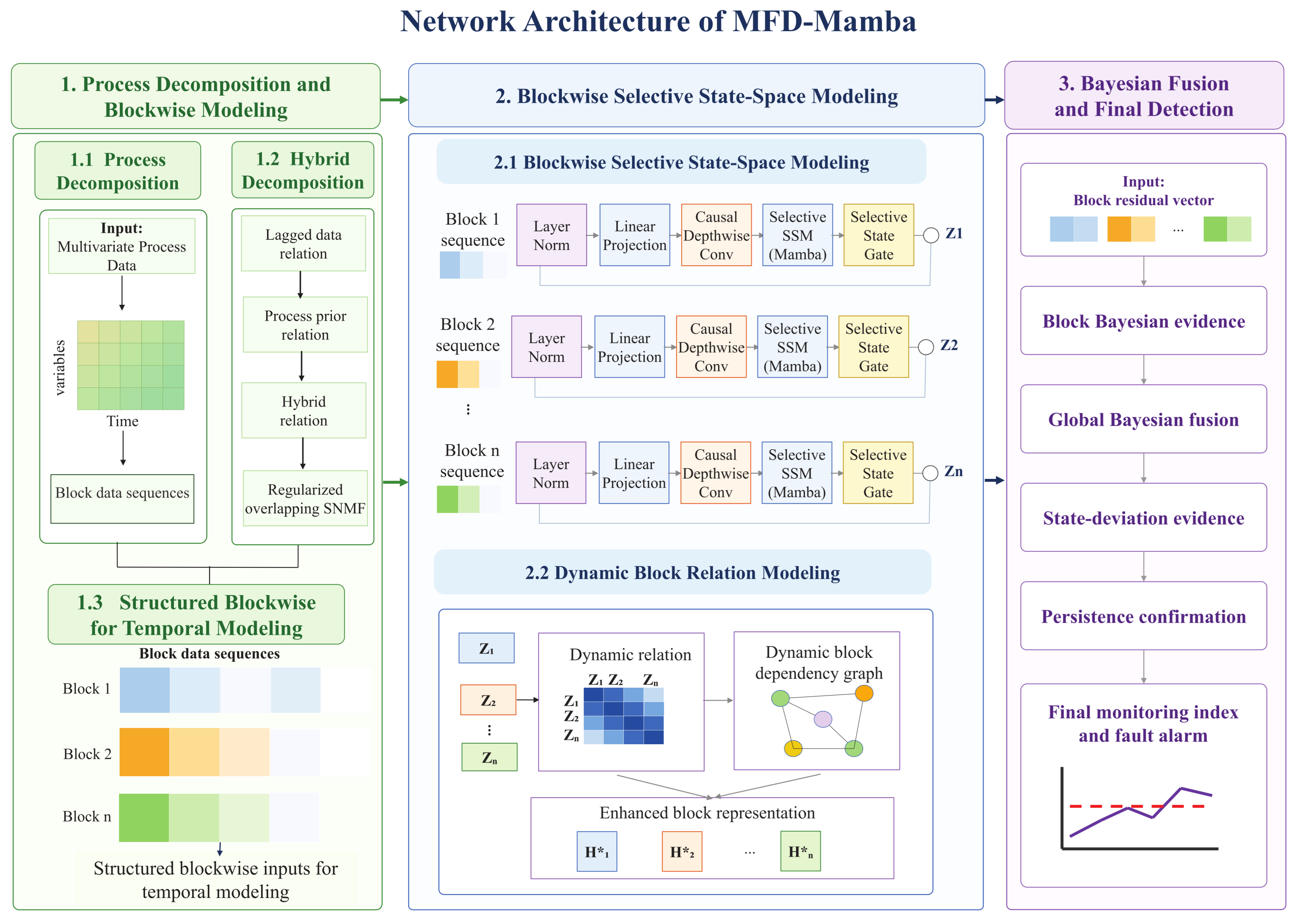
All control limits and evidence thresholds involved in the final decision are calibrated using normal operating data. No fault samples are used in the threshold determination. The resulting detector combines blockwise temporal prediction evidence with current-state deviations, providing a common monitoring decision for both simultaneous and sequential multiple-fault conditions. The overall framework is illustrated in Figure 1.

3.4. Hyperparameter Selection Strategy

The hyperparameters are selected in a staged manner according to their functional roles in the proposed framework. Parameters related to the multiblock construction are first adjusted to obtain stable and physically meaningful block structures. After the block structure is fixed, the parameters associated with temporal modeling and relation learning are determined based on the prediction behavior and the stability of the monitoring statistics. Finally, the smoothing-related parameter is selected to balance fault sensitivity and the suppression of isolated fluctuations. This staged strategy reduces the coupling among parameters from different modules and avoids simultaneously tuning all hyperparameters.

4. Two Industrial Cases

4.1. Experimental Settings

In this study, all computational efficiency experiments are conducted on the same Windows 11 workstation equipped with a 13th Gen Intel Core i7-13620H CPU, 15.73 GB of system memory, and an NVIDIA GeForce RTX 4060 Laptop GPU with 8 GB of memory. The experiments use Python 3.12.3 and PyTorch 2.13.0. The hyperparameters are selected in a staged manner according to their roles in the proposed framework. Specifically, ${\lambda }_p$, ${\lambda }_s$, and ${\lambda }_n$, which respectively control the contribution of process prior information, membership sparsity, and the penalty on non-mechanistic relations, are first determined to obtain stable and physically meaningful overlapping process blocks. After the block structure is fixed, ${\lambda }_r$, ${\lambda }_c$, and $\gamma$ are adjusted by considering the prediction performance and the stability of the resulting monitoring statistics. The EWMA smoothing coefficient ${\lambda }_e$ is selected to balance detection sensitivity and the suppression of isolated fluctuations, and ${\lambda }_e=0.40$ is used in the experiments. The corresponding detection thresholds are subsequently calibrated using normal operating data. Parameter selection is conducted using the training and validation data, while the test fault scenarios are reserved for final performance evaluation. This staged strategy avoids simultaneously tuning a large number of parameters and reduces the interactions among parameters belonging to different modules. For reproducibility, the final hyperparameter settings are summarized in

Table 1. Hyperparameter settings of MFD-Mamba for the TE process and ASP.

Hyperparameter	Symbol	TE	ASP
Process-prior weight	${\lambda }_p$	0.45	0.45
Sparsity coefficient	${\lambda }_s$	0.015	0.015
Non-prior penalty	${\lambda }_n$	0.08	0.08
Residual-tail weight	$\gamma$	0.30	0.30
Consistency weight	${\lambda }_c$	0.05	0.05
Relation-prior strength	${\lambda }_r$	0.75	0.75
EWMA smoothing coefficient	${\lambda }_e$	0.40	0.40
Fault prior	${\pi }_F$	0.01	0.01
Number of process blocks	B	4	4
Membership threshold	$\delta$	0.30	0.30
Block control confidence level	${\alpha }_b$	0.99	0.99
Global calibration confidence level	${\alpha }_g$	0.99	0.995
EWMA confidence level	${\alpha }_e$	0.999	0.999
Global Bayesian persistence	$K/N$	$2/3$	$2/3$
Moderate Mahalanobis persistence	$K/N$	$2/3$	$2/3$
Cross-evidence persistence	$K/N$	$2/2$	$2/2$

.

4.2. Tennessee Eastman Process

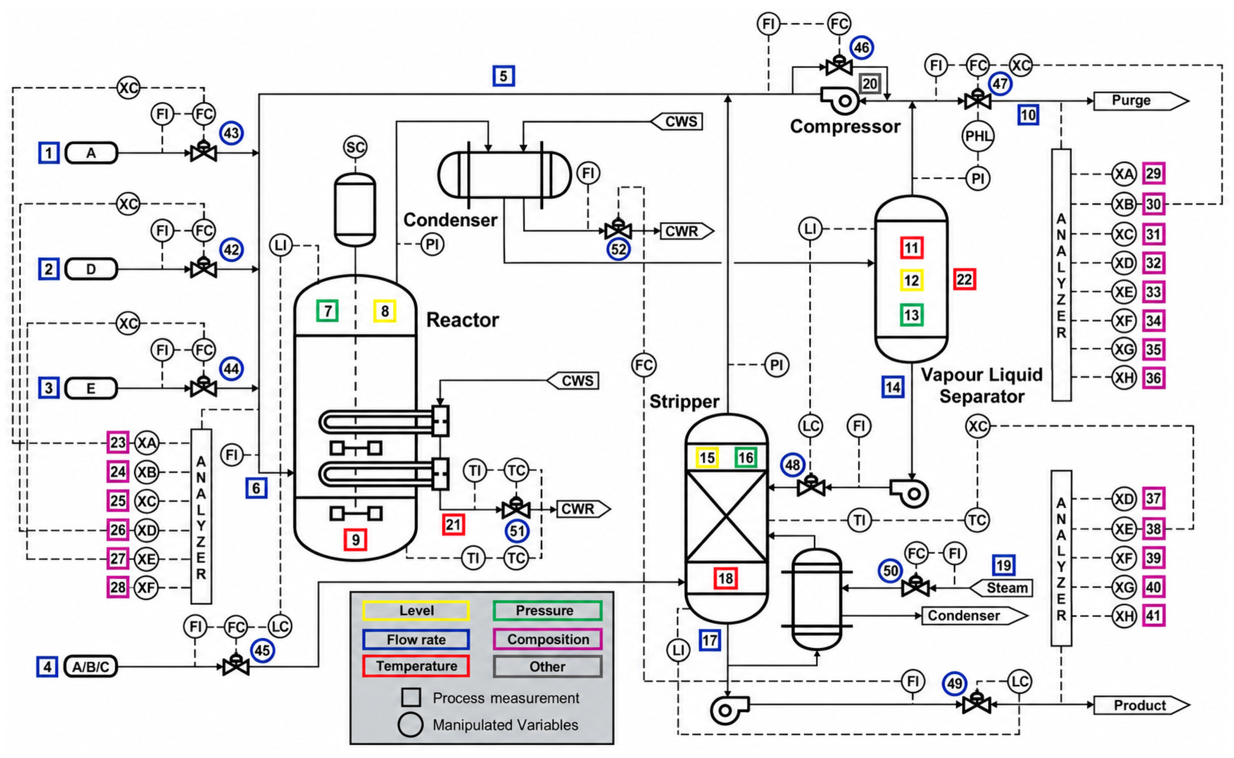
The Tennessee Eastman (TE) process is adopted as the benchmark system for evaluating the proposed monitoring framework [31]. As shown in Figure 2, the TE process consists of five major operating units, including a reactor, condenser, compressor, separator, and stripper. The benchmark provides a set of representative fault conditions with different dynamic characteristics, making it suitable for assessing monitoring performance under complex process disturbances. For the TE experiments, 33 variables are used as the input of the monitoring model, comprising 22 process measurements and 11 manipulated variables. Model training and control-limit estimation are both performed using normal-operation samples. The fault sequences are excluded from model construction and are introduced only during the testing stage. In this way, the detection results reflect the response of the trained model to previously unseen abnormal operating conditions.

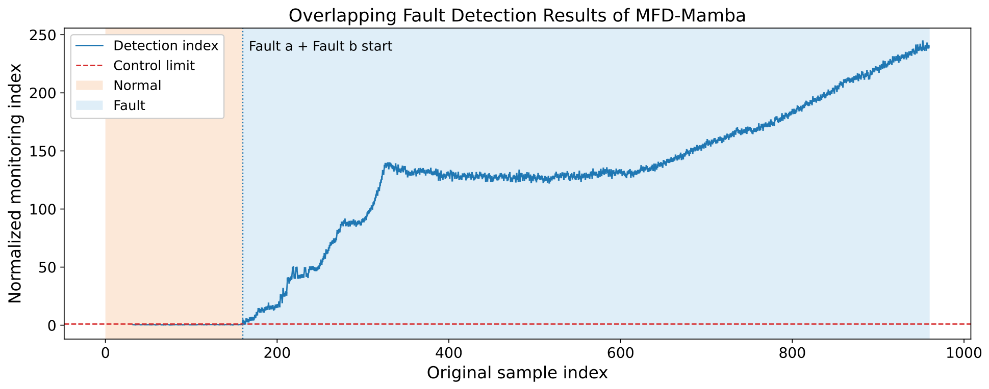
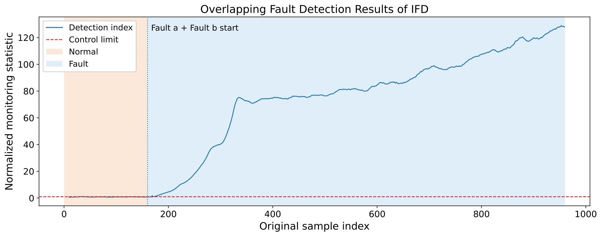
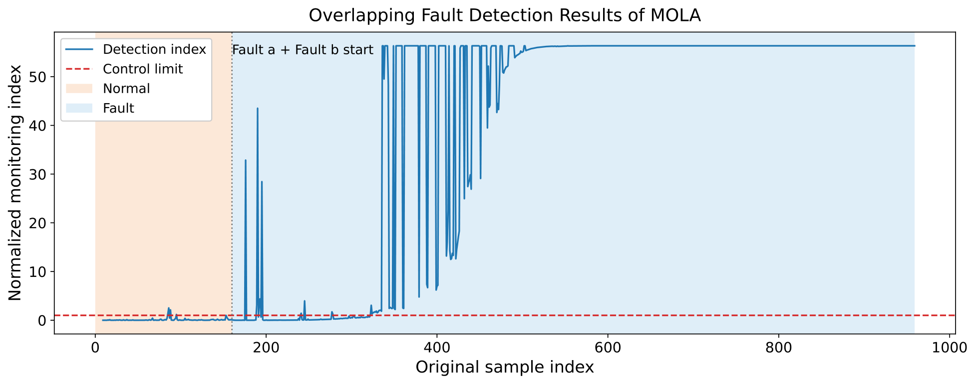
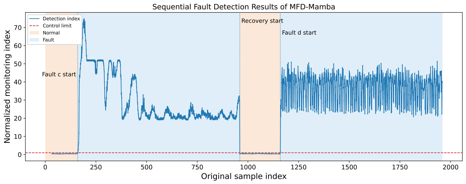
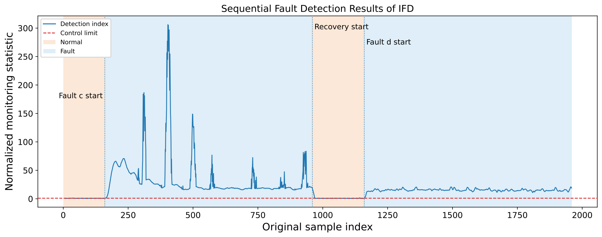
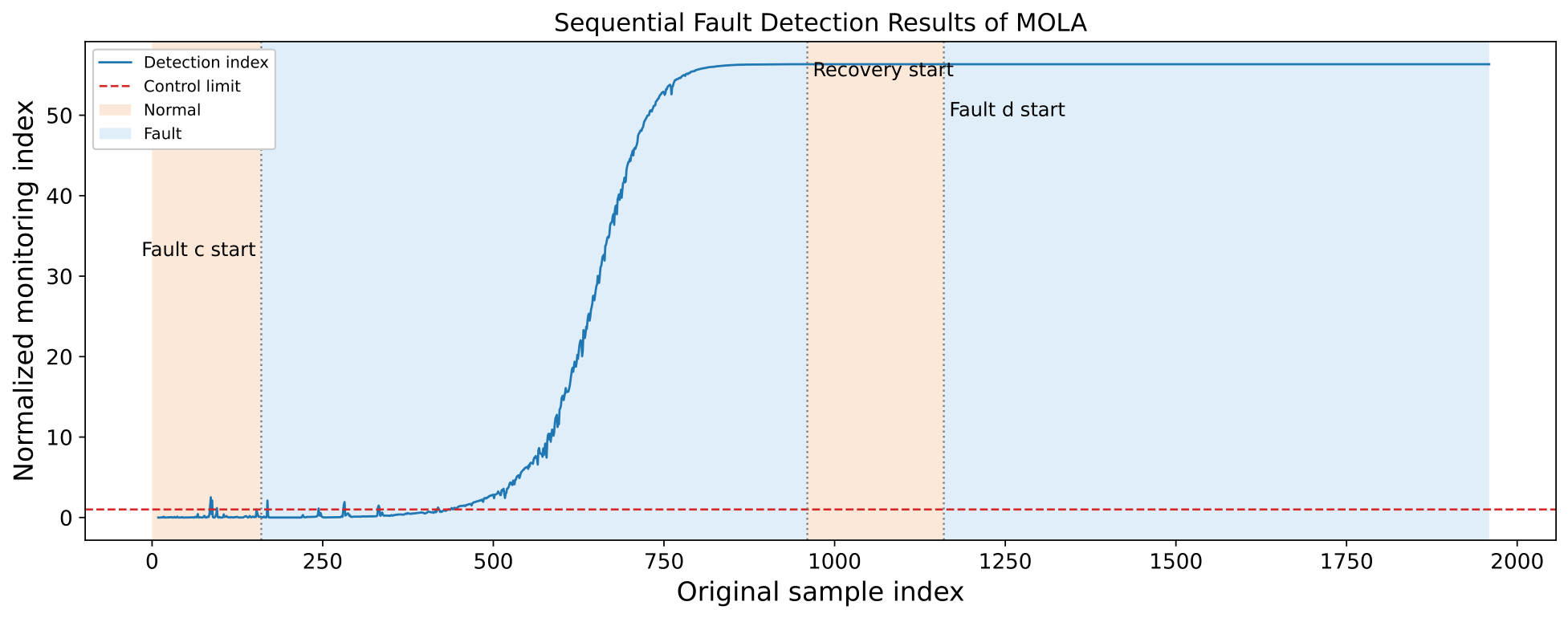
To further evaluate the monitoring performance under multiple-fault conditions, two scenarios are considered, namely, overlapping and sequential faults. For the overlapping-fault scenario, the first 160 samples represent normal operation. Fault 4 and Fault 6 are then introduced simultaneously from the 161st sample onward and remain active throughout the subsequent fault period. Concurrent-fault detection performance is evaluated under conditions where multiple fault effects coexist. For the sequential-fault scenario, the first 160 samples correspond to normal operation, followed by 800 samples affected by Fault 1. The process then returns to the normal condition for 200 samples to form a recovery interval, after which Fault 14 is introduced for the remaining 800 samples. Sequential-fault monitoring performance is evaluated in terms of the ability to track the transition from normal operation to a fault condition, recover after fault removal, and respond promptly to a subsequent fault of a different type.

For quantitative evaluation, the fault detection rate (FDR), false alarm rate (FAR), and detection delay are adopted as the performance metrics. The proposed MFD-Mamba is compared with MambaAD [27]; Mola [22], a multi-view Mamba-based method for multivariate time-series anomaly detection; and the incipient fault detection (IFD) method [32]. All methods are evaluated using the same test sequences and fault occurrence settings. The method-specific hyperparameters are configured according to their respective implementations, while the data partition and evaluation criteria are kept consistent across all methods to ensure a fair comparison. For the TE experiments, the input sequence length is set to 10 and the batch size is 32. The proposed model is trained for 50 epochs using the Adam optimizer with an initial learning rate of $3\times {10}^{-4}$. The control limit is determined from the normal training data with a confidence level of 0.99. A moving-average window of five samples is further employed to suppress isolated fluctuations in the monitoring statistic. All experiments are implemented under the same data partition and fault setting protocol.

Figure 3, Figure 4, Figure 5 and Figure 6 compare the detection performance of MFD-Mamba, MambaAD, IFD, and MOLA under the overlapping-fault scenario. As shown in Figure 3, the monitoring index of MFD-Mamba remains below the control limit during normal operation and rapidly enters the abnormal region after the overlapping faults occur, where it remains stable throughout the fault period. The detection result of MambaAD is shown in Figure 4. Its anomaly score increases gradually after fault occurrence and crosses the control limit after a transition period, resulting in a longer detection delay. As shown in Figure 5, IFD also responds to the overlapping faults, but several threshold exceedances occur during normal operation, leading to a higher FAR. MOLA, shown in Figure 6, exhibits a more fluctuating and intermittent response after fault occurrence, particularly during the early fault stage, indicating less stable fault detection.

Figure 7, Figure 8, Figure 9 and Figure 10 compare the detection performance of MFD-Mamba, MambaAD, IFD, and MOLA under the sequential-fault scenario. MFD-Mamba clearly tracks the successive transitions from normal operation to the first fault, recovery, and the second fault, with distinct changes in the monitoring index. In Figure 8, MambaAD also identifies the two fault stages and returns to the normal region during the recovery interval, although its response to the fault transitions is relatively slower. In Figure 9, IFD responds to both faults, but its monitoring statistic exhibits larger fluctuations and several pronounced peaks during the first fault stage.

In contrast, MOLA shows a delayed increase after the first fault occurs in Figure 10. Its monitoring index remains at a high level during the recovery interval, making the recovery and subsequent fault transition less distinguishable. MFD-Mamba provides clearer and more stable tracking of the successive operating-state transitions under the sequential-fault condition.

To examine the effect of training randomness, each method is independently trained and evaluated over six runs using six different random seeds. The same set of random seeds is used for all compared methods to enable paired statistical testing. The FDR, FAR, and detection delay are reported as the mean ± standard deviation, and a paired t-test is conducted on the seed-matched FDR results.

The quantitative results are summarized in

Table 2. Fault detection performance of different methods for the TE process, reported as mean ± standard deviation over six independent runs.

Method	Fault Scenario	FDR (%)	FAR (%)	Delay
MFD-Mamba	Overlapping fault	99.88 ± 0.03	0.13 ± 0.01	0 ± 0.00
Single-block Mamba	Overlapping fault	97.69 ± 0.82	8.98 ± 4.19	9.00 ± 0.00
MambaAD	Overlapping fault	98.75 ± 0.70	0.30 ± 0.08	39 ± 5.64
IFD	Overlapping fault	95.13 ± 0.11	7.28 ± 3.44	9 ± 2.16
MOLA	Overlapping fault	85.69 ± 6.97	2.21 ± 1.30	37.17 ± 31.51
MFD-Mamba	Sequential fault	99.81 ± 0.02	0.20 ± 0.06	2 ± 0.00/0 ± 0.10
Single-block Mamba	Sequential fault	98.88 ± 0.66	7.66 ± 3.35	8.00 ± 0.00/1.00 ± 0.00
MambaAD	Sequential fault	99.25 ± 2.09	1.35 ± 1.02	7 ± 0.98/2 ± 0.52
IFD	Sequential fault	98.56 ± 0.03	3.81 ± 2.10	2 ± 0.41/1 ± 0.50
MOLA	Sequential fault	94.70 ± 4.64	56.82 ± 0.58	15.67 ± 13.78/3 ± 0.80

Note: Bold values indicate the best-performing results.

. MFD-Mamba provides the best overall performance under both overlapping-fault and sequential-fault conditions, showing consistently high detection accuracy, low false alarm rates, and short detection delays. Compared with single-block Mamba, the proposed method achieves more reliable monitoring, particularly in terms of false alarm suppression and fault-response speed. This comparison indicates that the performance improvement does not arise from the Mamba backbone alone but also benefits from the proposed multiblock decomposition and fusion strategy. As shown in

Table 3. Statistical significance analysis of the FDR on the TE process.

Fault Scenario	Comparison	p-Value	Significance
Overlapping	MFD-Mamba vs. Single-block Mamba	0.0012	**
	MFD-Mamba vs. MambaAD	0.0108	*
	MFD-Mamba vs. IFD	<0.0001	***
	MFD-Mamba vs. MOLA	0.0042	**
Sequential	MFD-Mamba vs. Single-block Mamba	0.0182	*
	MFD-Mamba vs. MambaAD	0.5406	n.s.
	MFD-Mamba vs. IFD	<0.0001	***
	MFD-Mamba vs. MOLA	0.0429	*

* p < 0.05, ** p < 0.01, *** p < 0.001; n.s. denotes no statistically significant difference.

, the FDR improvements over MambaAD, IFD, and MOLA are statistically significant under the overlapping-fault condition. Under the sequential-fault condition, the difference between MFD-Mamba and MambaAD is not statistically significant, whereas significant differences are observed relative to IFD and MOLA. Overall, the results demonstrate that MFD-Mamba improves the selectivity and reliability of fault evidence while maintaining high sensitivity to multiple-fault transitions.

4.3. Activated Sludge Process

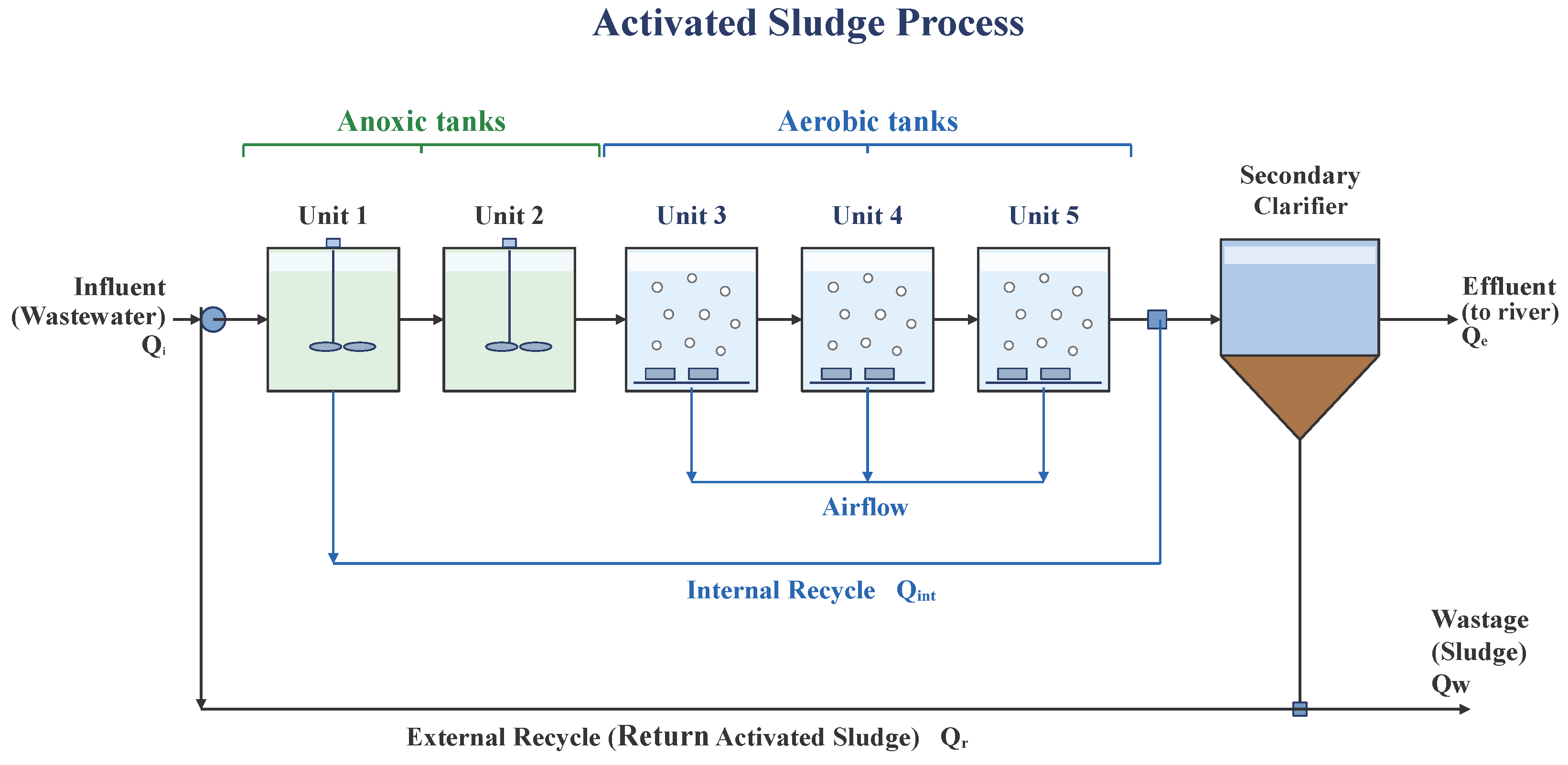
The activated sludge process (ASP) is used to evaluate the monitoring performance of the proposed method. The ASP plant consists of five biological reactors connected in series, followed by a secondary settler [33]. The first two reactors are operated under anoxic conditions for denitrification, whereas the remaining three reactors are aerated for carbon removal and nitrification. The secondary settler separates the treated effluent from activated sludge and includes return-sludge and waste-sludge streams. An internal recycle stream connects the aerobic and anoxic sections to support nitrogen removal. The biological reactions are described by ASM1, while the secondary settler is represented by a ten-layer settling model. A total of 25 process variables are selected as model inputs, and the effluent total nitrogen is retained as the quality variable. Normal operating data under dry, rainy, and storm conditions are used for model construction. The sampling interval is 15 min, and each test sequence covers Day 7 to Day 14, giving 672 samples.

For all methods, the normal samples under dry, rainy, and storm conditions are used for model construction, with 80% of each sequence used for training and the remaining 20% for validation. For MFD-Mamba, the window length is set to 32. The Mamba feature dimension and state dimension are 32 and 8, respectively, with two Mamba layers, a convolution width of 3, an expansion factor of 2, and a dropout rate of 0.1. Four overlapping process blocks are used. The model is trained using AdamW with a learning rate of $3\times {10}^{-4}$, a batch size of 64, and a maximum of 80 epochs. For MambaAD, the window length is 64, with a patch length of 8 and an overlap of 4. The model and state dimensions are 64 and 32, respectively. The learning rate is $1\times {10}^{-4}$, the batch size is 64, and the number of training epochs is 80. The temporal and signal masking ratios are both set to 0.1. For IFD, the window length and latent dimension are set to 10 and 32, respectively. The neighborhood sizes of the multiscale graph are 8, 16, and 24. The graph and stability regularization coefficients are set to 0.02 and 0.001. The model is trained for 200 epochs using Adam with a learning rate of $1\times {10}^{-3}$. The control limits are estimated from normal validation data with a confidence level of 0.99.

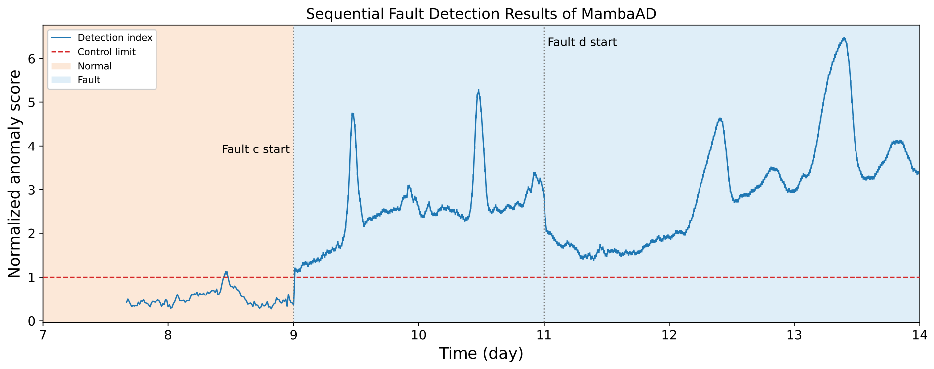
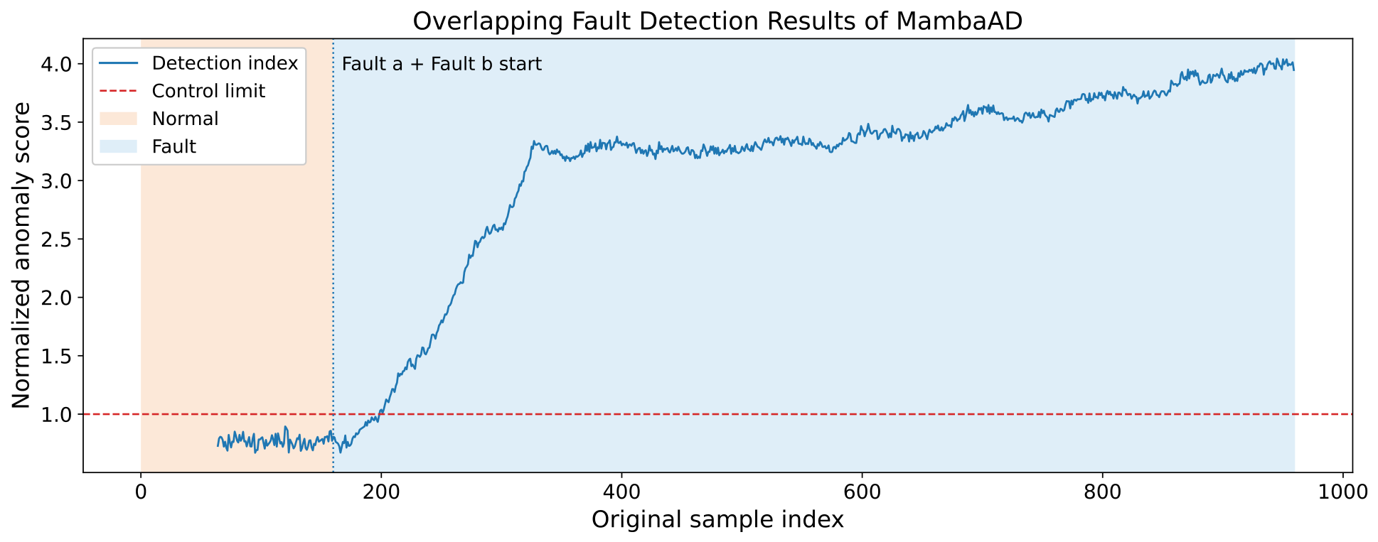
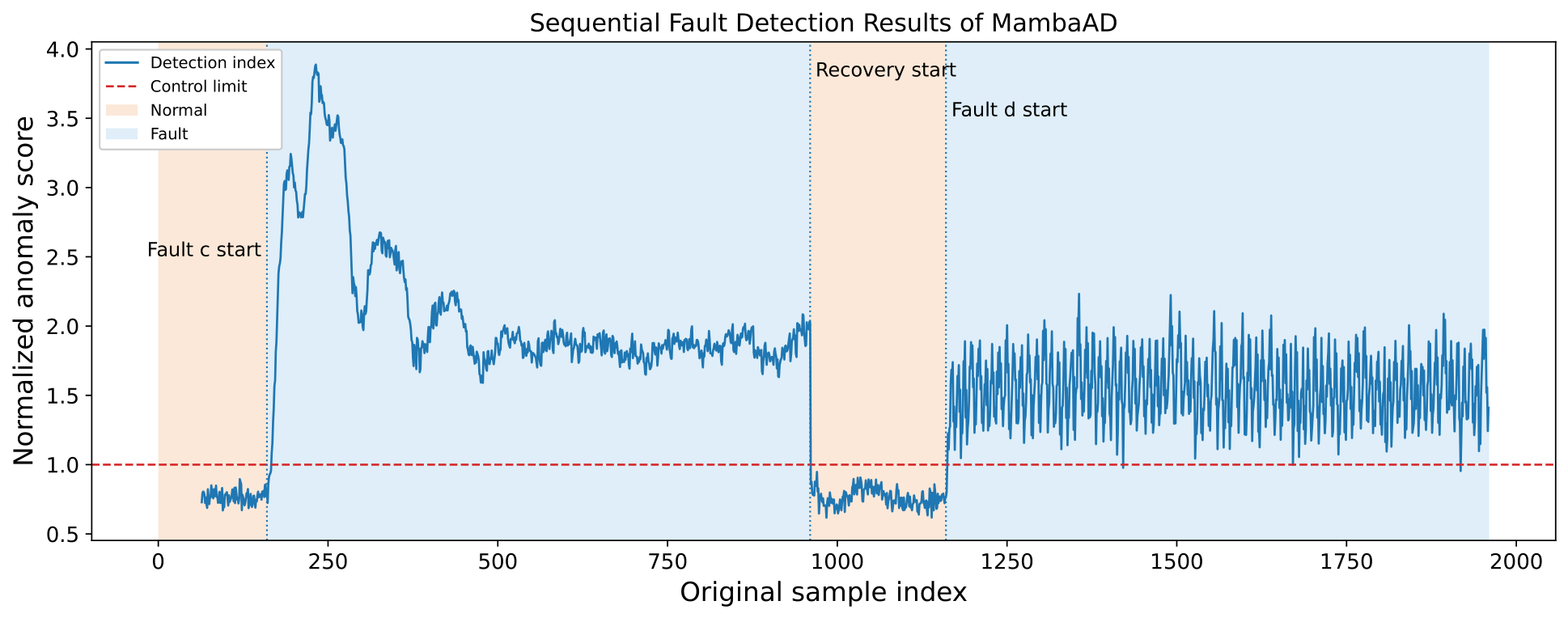
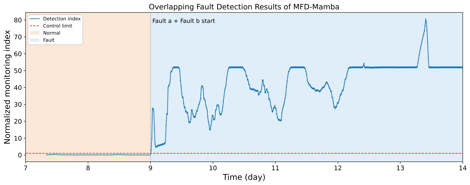
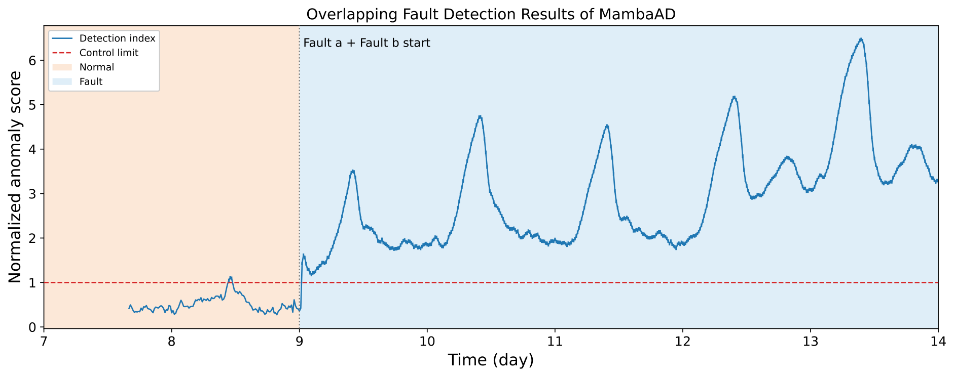
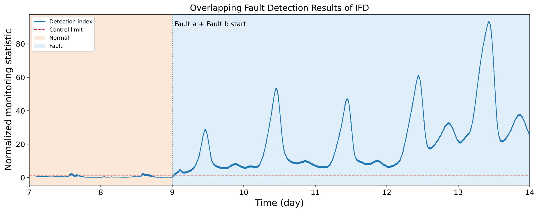
Two multiple-fault scenarios are considered, including overlapping and sequential faults. In the overlapping-fault scenario, Fault a and Fault b are introduced simultaneously. Fault a represents an aeration loss condition in which the oxygen transfer coefficient in the third aeration tank, $KL{a}_3$, is reduced from 240 to 120 d⁻¹. Fault b represents an influent nitrate shock, where the influent $S_{NO}$ is increased by 15 mgN/L. For the sequential-fault scenario, Fault c is followed by Fault d. Fault c represents an influent organic load shock, where the influent $S_S$ and $X_S$ are increased to twice their normal values. Fault d represents an influent nitrate shock, with the influent $S_{NO}$ increased by 15 mgN/L. No recovery interval is introduced between the two fault stages. Figure 11 presents the schematic structure of the ASP, including the biological reaction units, secondary clarifier, and internal recycle streams.

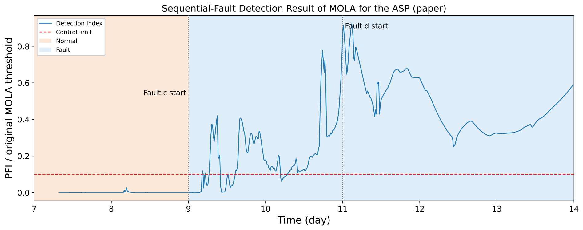
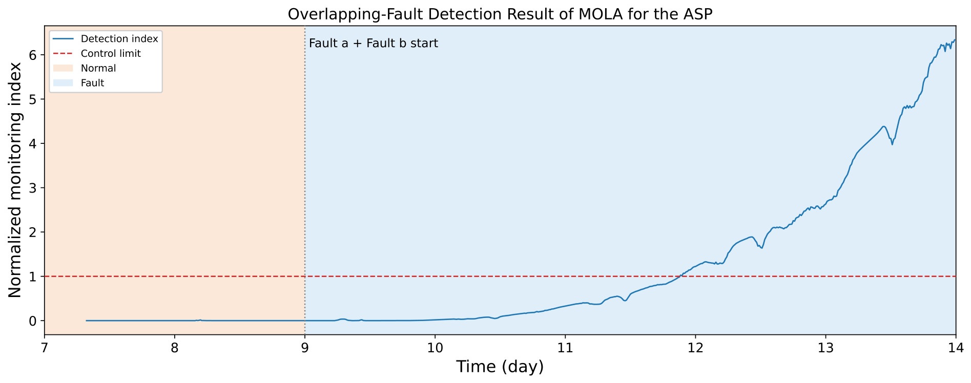
Figure 12, Figure 13, Figure 14 and Figure 15 compare the detection performance of MFD-Mamba, MambaAD, IFD, and MOLA under the overlapping-fault condition. MFD-Mamba responds rapidly after fault onset and maintains a clear separation between the normal and faulty operating regions. In Figure 13, MambaAD also detects the overlapping faults, although a short threshold crossing occurs during normal operation. IFD exhibits larger fluctuations and several threshold exceedances before fault occurrence, indicating a higher tendency toward false alarms in Figure 14. In Figure 15, MOLA shows a relatively slow increase after fault onset and crosses the control limit only after a noticeable transition period, resulting in a longer detection delay.

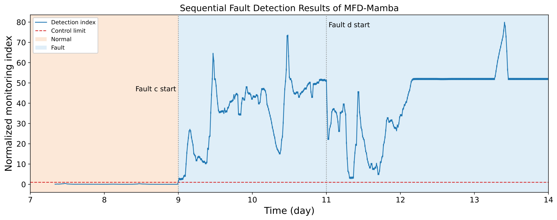
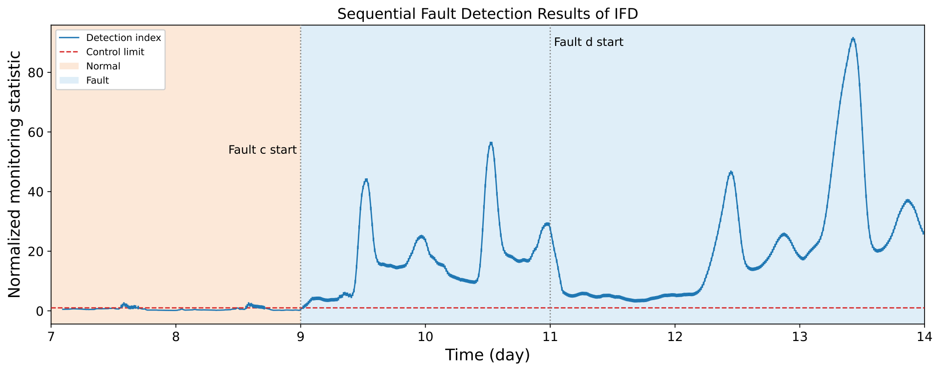
Figure 16, Figure 17, Figure 18 and Figure 19 compare the detection performance of MFD-Mamba, MambaAD, IFD, and MOLA under the sequential-fault condition. MFD-Mamba responds promptly to the first fault and maintains a clear abnormal response after the transition to the second fault in Figure 17. MambaAD also detects both fault stages, but its monitoring index exhibits larger variations around the fault transitions. IFD shows several pronounced peaks and stronger fluctuations during the sequential-fault period in Figure 18. MOLA responds to the faults, but exhibits a more irregular monitoring trajectory, particularly around the transition between the two fault stages.

The quantitative results are summarized in

Table 4. Fault detection performance of different methods for the ASP.

Method	FDR (%)	FAR (%)	Delay
Overlapping fault
MFD-Mamba	99.79 ± 0.01	0.78 ± 0.01	1 ± 0.00
Single-block Mamba	95.58 ± 2.50	9.38 ± 3.38	8.00 ± 0.00
MambaAD	99.37 ± 0.76	2.34 ± 1.48	3 ± 0.00
IFD	98.95 ± 0.11	15.30 ± 5.67	5 ± 0.52
MOLA	82.23 ± 6.37	9.21 ± 0.51	10.80 ± 3.16
Sequential fault
MFD-Mamba	99.58 ± 0.03	1.56 ± 0.07	0 ± 0.00/2 ± 0.00
Single-block Mamba	96.79 ± 2.38	10.62 ± 6.41	10.00 ± 0.00/8.00 ± 0.00
MambaAD	99.17 ± 2.52	2.34 ± 1.48	3 ± 2.66/0 ± 0.00
IFD	98.96 ± 0.32	15.30 ± 5.67	3 ± 0.00/2 ± 0.00
MOLA	82.23 ± 8.98	11.21 ± 1.51	3.75 ± 0.90/7.75 ± 1.01

Note: Bold values indicate the best-performing results.

. MFD-Mamba provides the best overall performance under both overlapping-fault and sequential-fault conditions, with consistently high detection accuracy, low false alarm rates, and short detection delays. As shown in

Table 5. Statistical significance analysis of the FDR on the ASP.

Fault Scenario	Comparison	p-Value	Significance
Overlapping	MFD-Mamba vs. Single-block Mamba	0.0091	**
	MFD-Mamba vs. MambaAD	0.0313	*
	MFD-Mamba vs. IFD	0.1250	n.s.
	MFD-Mamba vs. MOLA	0.0313	*
Sequential	MFD-Mamba vs. Single-block Mamba	0.0349	*
	MFD-Mamba vs. MambaAD	0.0313	*
	MFD-Mamba vs. IFD	0.0313	*
	MFD-Mamba vs. MOLA	0.0313	*

* $p<0.05$, ** $p<0.01$; n.s. denotes no statistically significant difference.

, the FDR improvements over MambaAD and MOLA are statistically significant under the overlapping-fault condition, whereas the difference relative to IFD is not significant. The comparison with single-block Mamba also shows a significant improvement, supporting the contribution of the proposed multiblock decomposition and fusion strategy.

Under the sequential-fault condition, significant FDR improvements are observed over all comparison methods, including single-block Mamba. Although some competing methods achieve relatively high FDRs, they generally exhibit higher false alarm rates or longer detection delays. The ASP results indicate that the performance gain does not arise from the Mamba backbone alone. The proposed multiblock decomposition and fusion strategy improves fault evidence selectivity and monitoring reliability under multiple-fault conditions.

4.4. Computational Efficiency Analysis

To evaluate the computational cost of the different methods, the number of trainable parameters, model size, total training time, and per-sample inference time are measured for MFD-Mamba, Transformer, MambaAD, IFD, and MOLA. Training time is measured as the wall-clock time required to complete the corresponding training procedure. For inference-time measurement, the batch size is set to one. After 50 warm-up runs, the average latency is calculated over 500 forward passes. Data loading and preprocessing are excluded from the inference-time measurement. The reported computational costs correspond to the sequence length adopted by each method in the fault detection experiments. For the TE process, the sequence lengths of MFD-Mamba, Transformer, MambaAD, IFD, and MOLA are 32, 32, 64, 10, and 10, respectively. For the ASP, the corresponding sequence lengths are 32, 32, 64, 10, and 32.

In addition to the empirical measurements, the computational complexity with respect to sequence length is considered. Let L denote the sequence length, d the hidden dimension, N the state dimension, and B the number of process blocks. The self-attention operation in a standard transformer has a sequence-dependent computational complexity of approximately $\mathcal{O}\left(L^{2}d\right)$ due to the pairwise attention computation. In contrast, the selective state-space operation used by Mamba scales linearly with L, with an approximate complexity of $\mathcal{O}\left(LdN\right)$. Therefore, for MFD-Mamba, the dominant temporal modeling term over multiple process blocks is expressed approximately as $\mathcal{O}\left(BLdN\right)$. The subsequent block relation and evidence fusion operations depend mainly on the number of process blocks, and do not introduce a quadratic dependence on the sequence length.

As shown in

Table 6. Computational efficiency comparison of different methods on the TE process and ASP.

Dataset	Method	Parameters (K)	Model Size (MB)	Training Time (s)	Inference Time (ms/Sample)
TE	MFD-Mamba	36.77	0.158	15.56	4.378
	Transformer	27.65	0.115	9.95	0.286
	MambaAD	233.44	0.919	142.31	6.855
	IFD	72.17	0.280	7.80	0.051
	MOLA	12.19	0.059	11.01	1.034
ASP	MFD-Mamba	36.25	0.156	320.80	5.224
	Transformer	27.13	0.113	35.98	0.287
	MambaAD	221.37	0.873	500.35	5.792
	IFD	56.73	0.221	19.24	0.056
	MOLA	11.58	0.057	25.25	1.201

, MFD-Mamba remains compact in terms of parameter count and model storage. Its parameter count and model size are considerably lower than those of MambaAD on both datasets, and it also requires less training and inference time than MambaAD. The Transformer baseline exhibits lower empirical latency under the relatively short input windows used in the present experiments. MOLA also requires lower inference latency than MFD-Mamba. Therefore, the present results do not indicate that MFD-Mamba is the fastest method under short-sequence conditions; instead, the computational motivation for the Mamba architecture mainly lies in its linear dependence on sequence length, in contrast to the quadratic dependence of standard self-attention (see

Table 7. Sequence -length dependence of representative sequence models.

Model	Dominant Sequence Modeling Cost	Dependence on L
Transformer	$\mathcal{O}\left(L^{2}d\right)$	Quadratic
LSTM/GRU	$\mathcal{O}\left(L{d}^2\right)$	Linear
Mamba	$\mathcal{O}\left(LdN\right)$	Linear
MFD-Mamba	$\mathcal{O}\left(BLdN\right)$	Linear

).

These results demonstrate that MFD-Mamba achieves the reported multiple-fault detection performance with a compact model and millisecond-level CPU inference. Although its empirical runtime is higher than that of the Transformer baseline, IFD, and MOLA under the present short-window settings, its state-space sequence modeling avoids the quadratic sequence-length dependence of self-attention. The additional computational cost mainly arises from multiblock temporal modeling, dynamic block relation modeling, and the subsequent evidence fusion procedure.

4.5. Interpretability Analysis

The block-wise Bayesian structure of MFD-Mamba provides a direct form of model interpretability. Prior to global evidence fusion, each process block generates posterior fault evidence $P_{b,t}^F$, the magnitude of which reflects the contribution of the corresponding block to the detected abnormal condition. For a given operating stage ${\mathcal{T}}_s$, the mean Bayesian fault evidence is calculated as

$${\overline{P}}_{b,s}^F={\displaystyle \frac{1}{|{\mathcal{T}}_s|}}\sum _{t\in {\mathcal{T}}_s}{P}_{b,t}^F,$$

(33)

where the block with the largest ${\overline{P}}_{b,s}^F$ is regarded as the dominant contributing block.

As shown in

Table 8. Mean block-wise Bayesian fault evidence under representative multiple-fault scenarios.

Dataset	Operating Stage	Block 1	Block 2	Block 3	Block 4	Dominant Block
TE	Overlapping fault	0.890	0.940	0.944	0.937	Block 3
TE	First fault	0.984	0.262	0.324	0.411	Block 1
TE	Recovery	0.002	0.002	0.001	0.002	–
TE	Second fault	0.142	0.650	0.001	0.997	Block 4
ASP	Overlapping fault	0.899	0.933	0.632	0.711	Block 2
ASP	First fault	0.801	0.766	0.674	0.481	Block 1
ASP	Second fault	0.710	0.753	0.830	0.889	Block 4

Note: Bold values indicate the best-performing results.

, overlapping-fault conditions activate multiple process blocks, while the dominant contributing block can still be identified from the Bayesian evidence. Block 3 provides the strongest contribution in the TE process, whereas Block 2 is dominant in the ASP process.

Under the sequential-fault condition, the dominant Bayesian evidence changes with the operating stage. In the TE process, the dominant contribution shifts from Block 1 during the first fault to Block 4 during the second fault, while the block evidences decrease to near-zero levels during recovery. A similar transition from Block 1 to Block 4 is observed in the ASP process. These stage-wise changes illustrate how the Bayesian fault evidence evolves as the operating condition changes.

The block-wise evidence provides an interpretable indication of which process region contributes most strongly to the monitoring decision and supports block-level fault localization; however, variable-level localization requires an additional within-block contribution analysis, and is left for future work.

4.6. Sensitivity to the Number of Process Blocks

To evaluate the sensitivity of MFD-Mamba to the number of process blocks, B is varied from 2 to 6 on both the TE and ASP processes, while the remaining settings are kept unchanged. As shown in

Table 9. Sensitivity of MFD-Mamba to the number of process blocks B on the TE and ASP processes.

		Overlapping Fault			Sequential Fault
Dataset	$\mathit{B}$	FDR (%)	FAR (%)	Delay	FDR (%)	FAR (%)	Delay
TE	2	98.12	3.11	6	99.25	1.07	4/2
TE	3	99.26	1.22	2	99.25	0.84	4/2
TE	4	99.88	0.12	0	99.81	0.20	2/0
TE	5	99.88	0.12	0	99.81	0.20	2/0
TE	6	97.75	2.66	17	99.25	3.20	4/2
ASP	2	95.83	9.01	3	92.50	7.50	14/0
ASP	3	98.54	3.99	2	97.21	2.87	7/0
ASP	4	99.79	0.78	1	99.58	1.56	2/0
ASP	5	99.79	0.78	2	99.58	1.56	2/0
ASP	6	99.79	0.78	2	99.58	1.56	2/0

Note: Bold values indicate the best-performing results.

, the monitoring performance generally improves as B increases from 2 to 4.

On the TE process, $B=4$ and $B=5$ provide the best overall monitoring performance, whereas a further increase to $B=6$ leads to noticeable deterioration, particularly under the overlapping-fault condition. On the ASP, the performance improves markedly from $B=2$ to $B=4$, then remains relatively stable for larger values of B. These results indicate that an excessively small number of blocks may merge process regions with different dynamic characteristics, whereas an excessively large number of blocks may fragment correlated process information without providing additional monitoring benefits. Therefore, $B=4$ is adopted in the final configuration as a balance between monitoring performance and model simplicity.

4.7. Ablation Study

Ablation experiments are conducted on the TE process and the ASP to evaluate the contributions of the main components of MFD-Mamba. The Mamba module and Bayesian fusion strategy are examined on both processes, while the final detector and block fusion mechanism are further evaluated on the TE and ASP processes, respectively. The results are summarized in

Table 10. Ablation results of MFD-Mamba for the TE process.

Method	Fault Scenario	FDR (%)	FAR (%)	Delay
MFD-Mamba	Overlapping fault	99.88	0.13	0
W/o Mamba	Overlapping fault	96.25	3.75	30
W/o Bayesian fusion	Overlapping fault	98.13	1.88	9
W/o final detector	Overlapping fault	97.50	9.37	15
MFD-Mamba	Sequential fault	99.81	0.20	2/0
W/o Mamba	Sequential fault	99.25	5.63	7/2
W/o Bayesian fusion	Sequential fault	97.63	4.37	5/2
W/o final detector	Sequential fault	98.56	3.81	7/10

Note: Bold values indicate the best-performing results.

and

Table 11. Ablation results of MFD-Mamba for the ASP.

Method	Scenario	FDR (%)	FAR (%)	Delay
MFD-Mamba	Overlapping	99.79	0.78	1
W/o Bayesian fusion	Overlapping	98.25	2.60	5
W/o equal block fusion	Overlapping	91.67	4.17	2
W/o Mamba	Overlapping	89.38	1.04	9
MFD-Mamba	Sequential	99.58	1.56	0/2
W/o Bayesian fusion	Sequential	98.83	3.13	8/2
W/o equal block fusion	Sequential	96.25	5.45	2/5
W/o Mamba	Sequential	90.42	7.16	19/0

Note: Bold values indicate the best-performing results.

.

For the TE process, removing Mamba mainly degrades the fault detection rate and response speed, whereas removing Bayesian fusion increases the false alarm rate and detection delay. The final detector also plays an important role in alarm reliability. Similar trends are observed on the ASP, where both the removal of Mamba and the replacement of the structured block fusion mechanism lead to clear performance degradation. The results indicate that the performance gain of MFD-Mamba does not arise from the Mamba backbone alone. Mamba-based temporal modeling, multiblock organization, and evidence fusion provide complementary contributions to fault detection, response speed, and alarm reliability.

5. Conclusions

This paper has presented MFD-Mamba for multiple-fault process monitoring in dynamic industrial processes. The proposed framework combines hybrid process decomposition, blockwise selective state-space modeling, dynamic block relation modeling, and fault evidence fusion. Data-derived lagged relationships and prior process connections are used to construct soft variable memberships and block relation information. The resulting blockwise sequences are processed by a shared modified Mamba encoder, and the block representations are subsequently updated according to their current interactions. Blockwise prediction residuals are then integrated through Bayesian fusion and combined with state deviation and persistence information to form the final monitoring decision. The proposed method was evaluated on the TE and the ASP under overlapping and sequential multiple-fault conditions. Comparative experiments showed that MFD-Mamba maintained high fault detection rates while controlling false alarm rates and detection delays across the considered fault scenarios. The ablation results further showed that temporal modeling, block relation modeling, block-level fusion, and the final detection components contribute to different aspects of monitoring performance.

References

1. Gao, L.; Chen, Z.; Ji, H.; Niu, Y.; Dong, H. Correlation-Aided Neural Network for Distributed Process Monitoring of Large-Scale Industrial Automation Systems. IEEE Trans. Ind. Inform. 2025, 21, 9526–9537. [Google Scholar] [CrossRef] [Scilit]
2. Chen, Y.; Ma, H.; Wang, Y.; Liu, X.; Zhang, X. Deep Feature Correlation Analysis for KPI-Related Fault Detection with Missing Data. IEEE Trans. Autom. Sci. Eng. 2026, 23, 11340–11357. [Google Scholar] [CrossRef] [Scilit]
3. Huo, M.; Yin, S. Interpretable Fault Diagnosis for Industrial Processes: A Unified Perspective. Artif. Intell. Sci. Eng. 2026, 2, 101–120. [Google Scholar] [CrossRef] [Scilit]
4. Song, B.; Zhang, J.; Wang, L.; Shi, H.; Tao, Y.; Li, Z.; Zheng, C. Fault Path Tracing and Root Cause Diagnosis Based on Semifrozen Autoencoder. IEEE Trans. Instrum. Meas. 2026, 75, 3513310. [Google Scholar] [CrossRef] [Scilit]
5. Si, Y.; Wang, Y.; Zhou, D. Key-performance-indicator-related process monitoring based on improved kernel partial least squares. IEEE Trans. Ind. Electron. 2020, 68, 2626–2636. [Google Scholar] [CrossRef] [Scilit]
6. Song, Y.; Zhang, A. From black box to physically interpretable: Trustworthy computing for AI-driven decision-making and control. J. Autom. Intell. 2026, 5, 91–111. [Google Scholar] [CrossRef] [Scilit]
7. Luo, H.; Wu, S.; Li, L. A time-domain estimation of the ν-gap metric and stability margin with its application to attack defense in cyber-physical systems. Automatica 2025, 182, 112549. [Google Scholar] [CrossRef] [Scilit]
8. Sun, C.Y.; Yang, G.H. A Quality-Relevant Fault Diagnosis Scheme Aided by Enhanced Dynamic Just-in-Time Learning for Nonlinear Industrial Systems. IEEE Trans. Ind. Inform. 2024, 20, 7471–7480. [Google Scholar] [CrossRef] [Scilit]
9. Wu, T.; Wang, L.; Xu, X.; Su, L.; He, W.; Wang, X. An intelligent fault detection algorithm for power transmission lines based on multi-scale fusion. Intell. Robot. 2025, 5, 474–487. [Google Scholar] [CrossRef] [Scilit]
10. Li, K.; Feng, J.; Sun, C.; Jiang, Y. TF-LGNet: A Time-Frequency Guided Local-Global Feature Network for Nonintrusive Load Monitoring. IEEE Sens. J. 2026, 26, 17262–17272. [Google Scholar] [CrossRef] [Scilit]
11. Mishra, R.K.; Choudhary, A.; Fatima, S.; Mohanty, A.R.; Panigrahi, B.K. A Systematic Review on Advancement and Challenges in Multi-Fault Diagnosis of Rotating Machines. Eng. Appl. Artif. Intell. 2025, 156, 111306. [Google Scholar] [CrossRef] [Scilit]
12. Jiang, Y.; Zhang, Z.; Mei, Y.; Zhang, M.; Mo, J.; Zio, E. A Bias-Variance Balanced Solution for Vibration-Based Fault Diagnosis of Tunnel Boring Machine Main Bearing. IEEE Sens. J. 2026, 26, 21360–21368. [Google Scholar] [CrossRef] [Scilit]
13. Sun, R.; Yin, X.; Wang, R. Hybrid kernel deep orthogonal subspace analysis-based anomaly detection for key performance indicators. Chemom. Intell. Lab. Syst. 2026, 278, 105874. [Google Scholar] [CrossRef] [Scilit]
14. Lee, G.; Han, C.; Yoon, E.S. Multiple-Fault Diagnosis of the Tennessee Eastman Process Based on System Decomposition and Dynamic PLS. Ind. Eng. Chem. Res. 2004, 43, 8037–8048. [Google Scholar] [CrossRef] [Scilit]
15. Zhao, C.; Gao, F. Fault Subspace Selection Approach Combined with Analysis of Relative Changes for Reconstruction Modeling and Multifault Diagnosis. IEEE Trans. Control Syst. Technol. 2016, 24, 928–939. [Google Scholar] [CrossRef] [Scilit]
16. Ma, L.; Dong, J.; Peng, K.; Zhang, C. Hierarchical Monitoring and Root-Cause Diagnosis Framework for Key Performance Indicator-Related Multiple Faults in Process Industries. IEEE Trans. Ind. Inform. 2019, 15, 2091–2100. [Google Scholar] [CrossRef] [Scilit]
17. Ma, L.; Yang, P.; Peng, K. Multitask Learning Based Collaborative Modeling of Heterogeneous Data for Compound Fault Diagnosis in Manufacturing Processes. IEEE Trans. Ind. Inform. 2024, 20, 14174–14183. [Google Scholar] [CrossRef] [Scilit]
18. Zhou, K.; Tong, Y.; Wei, X.; Song, K.; Chen, X. A Novel Multi-Label Classification Deep Learning Method for Hybrid Fault Diagnosis in Complex Industrial Processes. Measurement 2025, 242, 115804. [Google Scholar] [CrossRef] [Scilit]
19. Zhu, C.; Liu, N.; Li, Z.; Li, Y.; Guo, J.; Ji, L.; Zhao, Y.; Shi, X.; Lan, X. A Multi-Label Domain Adaptation Method for Unseen Compound Fault Recognition in FCC Settler Catalyst Loss Processes. Process Saf. Environ. Prot. 2025, 203, 107885. [Google Scholar] [CrossRef] [Scilit]
20. Yang, C.; Cai, B.; Kong, X.; Zhang, R.; Gao, C.; Liu, X.; Shao, H.; Zhao, X. Fast and Stable Fault Diagnosis Method for Composite Fault of Subsea Production System. Mech. Syst. Signal Process. 2025, 226, 112373. [Google Scholar] [CrossRef] [Scilit]
21. Eydam, L.; Lange, H.; Urbas, L. Hybrid Fault Diagnosis in the Process and Chemical Industries: A Review. Annu. Rev. Control 2026, 62, 101064. [Google Scholar] [CrossRef] [Scilit]
22. Ma, F.; Ji, C.; Wang, J.; Sun, W.; Tang, X.; Jiang, Z. MOLA: Enhancing Industrial Process Monitoring Using a Multi-Block Orthogonal Long Short-Term Memory Autoencoder. Processes 2024, 12, 2824. [Google Scholar] [CrossRef] [Scilit]
23. Xue, C.; Zhang, T.; Xiao, D. Output Related Fault Detection and Diagnosis Based on Multi Block Modified Orthogonal Broyden-Fletcher-Goldfarb-Shanno Algorithm. Neurocomputing 2024, 607, 128350. [Google Scholar] [CrossRef] [Scilit]
24. Yan, S.; Yang, Y.; Ran, J.; Xiong, T.; Huang, H.; Zhu, J.; Yang, X.; Zhai, C.; Zhang, G.; Zhang, H. Fast and interpretable just-in-time learning via information-weighted similarity search: Probabilistic soft sensing of catalyst coke in MTO process. Chem. Eng. Sci. 2026, 330, 123911. [Google Scholar] [CrossRef] [Scilit]
25. Zhu, Z.; Chen, F.; Ni, L.; Bian, H.; Jiang, J.; Chen, Z. A Novel Transformer-Based Model with Large Kernel Temporal Convolution for Chemical Process Fault Detection. Comput. Chem. Eng. 2024, 188, 108762. [Google Scholar] [CrossRef] [Scilit]
26. Zhang, H.; Li, Y.; Zhang, X.; Feng, H. Multi-Scale Group Mamba Network with Structural Attention for Rotating Machinery Fault Diagnosis Using Multisensor Data. Adv. Eng. Inform. 2025, 67, 103521. [Google Scholar] [CrossRef] [Scilit]
27. Qin, S.; Zhu, J.; Guo, A.; Yang, Y.; Wang, L.; Tao, G. MambaAD: Multivariate time series anomaly detection in IoT via multi-view Mamba. Neurocomputing 2025, 655, 131385. [Google Scholar] [CrossRef] [Scilit]
28. Li, G.; Ge, M.; Wan, J.; Han, D.; Li, M.; Zhou, M. MemMambaAD: Memory-augmented state space model for multivariate time series anomaly detection. Eng. Appl. Artif. Intell. 2025, 158, 111308. [Google Scholar] [CrossRef] [Scilit]
29. Yang, P.; Xie, Z.; Sheng, S. Dual-path mamba for chemical process fault diagnosis with adaptive signal decomposition. Chin. J. Chem. Eng. 2026; in press. [CrossRef] [Scilit]
30. Mishra, R.K.; Choudhary, A.; Fatima, S.; Mohanty, A.R.; Panigrahi, B.K. Adaptive Information Fusion for Multi-Fault Diagnosis Using Multi-Stream Convolutional Neural Network. Measurement 2026, 272, 121043. [Google Scholar] [CrossRef] [Scilit]
31. Wang, G.; Yang, J.; Qian, Y.; Han, J.; Jiao, J. KPCA-CCA-Based Quality-Related Fault Detection and Diagnosis Method for Nonlinear Process Monitoring. IEEE Trans. Ind. Inform. 2023, 19, 6492–6501. [Google Scholar] [CrossRef] [Scilit]
32. Sun, C.; Wang, X.; Cheng, Y. A Quality-Related Incipient Fault Detection and Location for Industrial IoT with Incomplete Data. IEEE Internet Things J. 2026, 13, 23524–23536. [Google Scholar] [CrossRef] [Scilit]
33. Alex, J.; Benedetti, L.; Copp, J.; Gernaey, K.V.; Jeppsson, U.; Nopens, I.; Pons, M.N.; Steyer, J.P.; Vanrolleghem, P.A. Benchmark Simulation Model No. 1 (BSM1); Technical Report TEIE-7229; Lund University: Lund, Sweden, 2008. [Google Scholar]
Figure 1. Framework of the proposed MFD-Mamba method.
Processes 14 02973 g001
Figure 2. Schematic diagram of the Tennessee Eastman process.
Processes 14 02973 g002
Figure 3. Overlapping fault detection results of MFD-Mamba for TE.
Processes 14 02973 g003
Figure 4. Overlapping fault detection results of MambaAD for TE.
Processes 14 02973 g004
Figure 5. Overlapping fault detection results of IFD for TE.
Processes 14 02973 g005
Figure 6. Overlapping fault detection results of MOLA for TE.
Processes 14 02973 g006
Figure 7. Sequential fault detection results of MFD-Mamba for TE.
Processes 14 02973 g007
Figure 8. Sequential fault detection results of MambaAD for TE.
Processes 14 02973 g008
Figure 9. Sequential fault detection results of IFD for TE.
Processes 14 02973 g009
Figure 10. Sequential fault detection results of MOLA for TE.
Processes 14 02973 g010
Figure 11. Schematic diagram of the ASP.
Processes 14 02973 g011
Figure 12. Overlapping fault detection result of MFD-Mamba for the ASP.
Processes 14 02973 g012
Figure 13. Overlapping fault detection result of MambaAD for the ASP.
Processes 14 02973 g013
Figure 14. Overlapping fault detection result of IFD for the ASP.
Processes 14 02973 g014
Figure 15. Overlapping fault detection result of MOLA for the ASP.
Processes 14 02973 g015
Figure 16. Sequential fault detection result of MFD-Mamba for the ASP.
Processes 14 02973 g016
Figure 17. Sequential fault detection result of MambaAD for the ASP.
Processes 14 02973 g017
Figure 18. Sequential fault detection result of IFD for the ASP.
Processes 14 02973 g018
Figure 19. Sequential fault detection result of MOLA for the ASP.
Processes 14 02973 g019