Article

Transmission–Distribution Coordinated Multi-Time-Scale Rolling Optimal Control Considering Static Voltage Stability

1
State Grid Zhejiang Electric Power Co., Ltd. Research Institute, Hangzhou 310014, China
2
State Grid Zhejiang Electric Power Co., Ltd., Hangzhou 310007, China
3
State Grid Xiangshan Power Supply Company, Ningbo 315700, China
4
State Key Laboratory of Power Transmission Equipment Technology, School of Electrical Engineering, Chongqing University, Chongqing 400044, China
*
Author to whom correspondence should be addressed.
Processes 2026, 14(18), 2877; https://doi.org/10.3390/pr14182877
Submission received: 12 July 2026 / Revised: 27 August 2026 / Accepted: 4 September 2026 / Published: 9 September 2026
(This article belongs to the Section Energy Systems)

Abstract

The increasing penetration of distributed energy resources has strengthened the operational coupling between transmission and distribution grids, intensified voltage fluctuations, and reduced static voltage stability margins under bidirectional power-flow conditions. In transmission–distribution coordinated operation, conventional scheduling methods have difficulty simultaneously addressing boundary power interaction, renewable generation forecasting errors, real-time corrective control, and static voltage stability constraints. To address these issues, this paper proposes a transmission–distribution coordinated multi-time-scale rolling optimal control method considering static voltage stability. First, based on local network equivalencing, a static voltage stability index (SVSI) calculation method is developed for scenarios with bidirectional power-flow variations, enabling fast online assessment of static voltage stability boundaries. Second, the transmission–distribution boundary exchange power is selected as the key coordination variable, and a multi-time-scale rolling optimization framework is established to coordinate main-grid operational requirements with distribution-side flexible resources. At the long time scale, a baseline scheduling plan is generated by considering economic operation, renewable energy accommodation, and transmission–distribution boundary power exchange. At the short time scale, model predictive control (MPC) is adopted to perform closed-loop correction of control variables using rolling forecast information and real-time measurements, thereby achieving rolling coordinated control of distributed generation, energy storage systems, flexible regulation resources, and boundary exchange power. Furthermore, the SVSI is embedded into the rolling optimization model as a security constraint, forming a multi-objective coordinated control method that jointly considers economic performance, renewable energy accommodation capability, transmission–distribution interaction, and static voltage security margin. Case study results show that the proposed method can effectively improve renewable energy accommodation and reduce network losses while enhancing the static voltage stability margin. In addition, it improves the adaptability of the coordinated transmission–distribution system to operating-condition variations, forecasting deviations, and boundary power fluctuations.

1. Introduction

With the increasing penetration of distributed photovoltaics, wind power, energy storage systems, and flexible loads in distribution networks, conventional distribution networks are evolving from an operating mode characterized by unidirectional power reception and passive regulation toward one involving multi-source integration, bidirectional power flow, and active control. Existing studies have systematically analyzed the integration of distributed generation from the perspectives of its definition, integration benefits, operational challenges, and distribution network planning [1,2,3,4,5,6]. The integration of distributed generation can promote local renewable energy accommodation, reduce losses in certain feeders, and improve local power supply capability. However, the stochastic, intermittent, and fluctuating nature of distributed generation also changes the original power-flow distribution and nodal voltage profiles. Under high-penetration distributed generation scenarios, distribution networks may experience reverse power flow, intensified voltage fluctuations, rapid variations in operating conditions, and reduced static voltage stability margins. Therefore, achieving multi-time-scale rolling optimal control of distribution networks under uncertain renewable energy output, while simultaneously considering operational economy, renewable energy accommodation, and static voltage stability security, has become an urgent issue in the optimal operation of active distribution networks.
Model predictive control (MPC) provides rolling optimization, feedback correction, and explicit constraint-handling capabilities, and has been widely applied to the optimal scheduling and control of power systems with intermittent resources [7,8,9,10,11,12,13,14]. Su et al. [15] developed an MPC-based power scheduling model for distribution systems considering the uncertainty of plug-in electric vehicles, aiming to improve the adaptability of distribution systems to stochastic loads. Parisio et al. [16] applied MPC to microgrid operation optimization, thereby improving energy management capability under forecasting errors. Raimondi Cominesi et al. [17] proposed a two-layer stochastic MPC framework to realize optimal microgrid control across different time scales. More recently, MPC has also been extended to multifunctional control of voltage-source-converter-based microgrids under both islanded and grid-connected operating modes [18]. These studies indicate that MPC and related real-time dispatch methods can mitigate the impact of renewable energy fluctuations and load forecasting errors on scheduling results through rolling prediction and feedback correction [19]. However, existing multi-time-scale MPC scheduling models mainly focus on operating cost, power balance, renewable energy accommodation, or power tracking deviation as optimization objectives, while the explicit role of static voltage stability boundaries as constraints in the rolling optimization process remains insufficiently considered.
Static voltage stability analysis is an important basis for ensuring the secure operation of distribution networks with high-penetration distributed generation. Continuation power flow, modal analysis, power-flow solvability criteria, and line- or node-based static voltage stability indices have been widely used for voltage stability assessment [20,21,22,23,24,25]. Among these methods, the static voltage stability index (SVSI) has the advantages of a concise computational form, clear physical interpretation, and ease of integration into optimization models, making it suitable for online security assessment and scheduling constraint formulation. Song et al. [26] investigated the static voltage stability mechanism of distribution systems based on the network-load admittance ratio. Wang et al. [27] proposed a necessary condition for power-flow insolvability in distribution systems with distributed generators. Aolaritei et al. [28] developed a hierarchical and distributed monitoring method for voltage stability in distribution networks. However, after the integration of high-penetration distributed generation, the power-flow directions around a node may vary with renewable energy output, and some nodes may simultaneously have multiple power-inflow branches and multiple power-outflow branches. Traditional SVSI calculation methods based on a single branch power-flow direction are therefore unable to accurately characterize the equivalent electrical relationship of the local network around a node, which affects the accuracy of online static voltage stability boundary assessment.
In terms of coordinated scheduling models for distribution networks, existing studies generally incorporate factors such as operating cost, network losses, renewable energy accommodation, energy storage operation, and flexible load response into the objective function. The feasibility of scheduling schemes is usually ensured through power-flow constraints, nodal voltage constraints, branch capacity constraints, device operating constraints, and voltage management strategies [3,5,6,15,29,30]. Some studies have further introduced voltage stability indices or voltage stability margins into optimization models. Jalali and Aldeen [31] proposed a risk-based stochastic allocation method for energy storage systems to ensure the voltage stability margin of distribution systems. Eajal et al. [32] analyzed the loadability and voltage stability of islanded AC–DC hybrid microgrids during contingencies. Wang et al. [33] embedded steady-state voltage stability constraints into a semidefinite programming-based optimal power flow model, thereby improving the voltage stability security of the optimized operating results. Bakhtvar and Keane [34] considered long-term voltage stability constraints in wind capacity allocation. These studies are significant for improving the operational economy and security margins of distribution networks. Nevertheless, most of them focus on planning and allocation, offline assessment, or static optimization scenarios, and have not fully considered the coupling between online SVSI calculation results and the multi-time-scale rolling optimization process of MPC. Relying only on voltage magnitude constraints and power balance constraints cannot accurately reflect the distance between the system operating point and the static voltage stability boundary. As a result, a scheduling scheme may still involve potential voltage stability risks even when it achieves favorable economic performance.
Although the aforementioned studies have laid a foundation for improving the rolling scheduling capability of active distribution networks, characterizing static voltage stability boundaries, and exploiting the regulation potential of distributed resources, several limitations remain. First, existing multi-time-scale MPC scheduling studies mainly focus on renewable energy accommodation, operating cost, and power tracking, while insufficient attention has been paid to the time-varying constraints imposed by static voltage stability margins. Second, existing SVSI methods are mostly used for security assessment, planning and allocation, or static optimization, and have not been sufficiently combined with real-time measurements and rolling forecast information to update static voltage stability boundaries online. Third, existing coordinated scheduling models usually adopt voltage magnitude constraints as the primary security constraints, making it difficult to reflect the actual distance between the system operating point and the static voltage stability boundary. Therefore, embedding an online SVSI calculation method applicable to bidirectional power-flow scenarios into the multi-time-scale MPC rolling optimal control process can more fully exploit the coordinated regulation capability of distributed generation, energy storage systems, and flexible loads [35], thereby further improving the operational economy, renewable energy accommodation capability, and static voltage security level of distribution networks.
To address these issues, this paper proposes a multi-time-scale rolling optimal control method for distribution networks considering static voltage stability. First, an MPC-based multi-time-scale coordinated scheduling framework for distribution networks is developed. Through the coordination of long-time-scale baseline scheduling, short-time-scale rolling optimization, and real-time feedback correction, the adaptability of the scheduling strategy to renewable energy fluctuations and load forecasting errors is improved. Second, based on the concept of local network equivalencing, an online SVSI calculation method applicable to bidirectional power-flow scenarios is established, enabling fast assessment of static voltage stability boundaries in distribution networks. Furthermore, the SVSI is embedded into the MPC rolling optimization model as a security constraint, forming a coordinated control method that simultaneously considers operational economy, renewable energy accommodation, and static voltage stability margin. The main contributions of this paper are summarized as follows:
In this study, each MPC sampling instant is treated as a quasi-steady-state operating point, and the proposed SVSI evaluates static voltage stability at that operating point. Dynamic or transient voltage stability is beyond the scope of this study.
(1)
An MPC-based multi-time-scale coordinated scheduling framework for distribution networks is proposed. By coordinating the long-time-scale baseline schedule with short-time-scale rolling correction, the proposed framework realizes closed-loop scheduling control under renewable energy output fluctuations and load forecasting errors.
(2)
An online SVSI calculation method based on local network equivalencing is established. To address the complex variations in power-flow directions around nodes after the integration of high-penetration distributed generation, the local network is equivalently processed, enabling fast assessment of the static voltage stability index under bidirectional power-flow scenarios.
(3)
An MPC-based coordinated scheduling model for distribution networks considering static voltage stability constraints is constructed. The online calculated SVSI is embedded into the rolling optimization process, allowing the scheduling strategy to account for economic performance, renewable energy accommodation, and scheduling smoothness while preventing the system operating point from approaching the static voltage stability boundary.
The remainder of this paper is organized as follows. Section 2 establishes the MPC-based multi-time-scale coordinated scheduling framework for distribution networks. Section 3 proposes the SVSI calculation method based on local network equivalencing. Section 4 constructs the coordinated scheduling model for distribution networks considering static voltage stability constraints. Section 5 verifies the effectiveness of the proposed method through case studies. Section 6 concludes the paper.

2. Multi-Time-Scale Coordinated Scheduling Framework for Distribution Networks Based on MPC

2.1. Basic Principles of Model Predictive Control

Model predictive control (MPC) is a model-based finite-horizon closed-loop optimization control method, which mainly consists of three components: a prediction model, rolling optimization, and feedback correction. The prediction model is used to predict system outputs over a finite horizon according to the current system state and future input information. Rolling optimization is performed to solve the optimal control sequence over the prediction horizon while satisfying the objective function and system constraints. Feedback correction uses real-time measurements to compensate for prediction errors, thereby enabling the next optimization cycle to better reflect the actual operating state of the system.
Let the current sampling instant be denoted by k , the prediction horizon by N , and the control horizon by M , where M ≤ N. At each sampling instant, MPC solves the sequence of control variables over the future control horizon based on the current system state and forecast information:
Δ u M k = Δ u T k + 1 k , Δ u T k + 2 k , , Δ u T k + i k , , Δ u T k + M k
where Δ u T k + 1 k denotes the vector of control variables predicted at time k for the future interval k + i 1 , k + i . MPC does not implement the entire control sequence at once. Instead, only the first element of the optimized control sequence is applied as the actual control action for the current sampling period. At the next sampling instant, the system acquires updated measurement information and forecast results, and a new control sequence is then solved. Therefore, MPC can continuously correct operating deviations during the rolling optimization process and prevent the accumulation of prediction errors over a long prediction horizon from having a persistent impact on subsequent control actions.
For distribution networks with high penetration of distributed generation, the advantage of MPC lies in its ability to use rolling forecasts of renewable generation and load to respond in advance to future operating-condition variations. Meanwhile, real-time measurement feedback is used to continuously correct forecasting errors, making the scheduling results more consistent with the actual system operation. Therefore, introducing MPC into the multi-time-scale scheduling process of distribution networks is beneficial for improving the adaptability of distribution networks to renewable power fluctuations and load uncertainties.

2.2. Multi-Time-Scale Coordinated Scheduling Architecture Considering the Transmission–Distribution Boundary

Different types of adjustable resources in distribution networks have distinct response speeds and scheduling characteristics. Controllable distributed generators, energy storage systems, and certain flexible loads have relatively fast response capabilities and are suitable for participating in short-time-scale rolling optimization. By contrast, on-load tap-changing transformers, reactive power compensation devices, and flexible loads that require advance notification are subject to limitations related to device lifetime, operating conditions, and user response time. These resources are therefore more suitable for forming baseline schedules over a longer time scale. Accordingly, distribution network scheduling should not rely on a single time scale to complete all control tasks. Instead, a coordinated architecture combining long-time-scale baseline scheduling and short-time-scale rolling correction should be established.
In the context of coordinated transmission–distribution operation, the distribution network exchanges power with the transmission network through the point of common coupling (PCC). Its distributed generators, energy storage systems, flexible loads, and other resources can, to some extent, participate in main-grid power regulation and voltage support. Therefore, this paper takes the power exchanged at the transmission–distribution boundary as the coordination variable between the long- and short-time-scale scheduling stages. In this way, both the long-time-scale baseline schedule and the short-time-scale rolling correction can reflect the regulation capability of distribution-side resources and the variation in transmission–distribution boundary power.
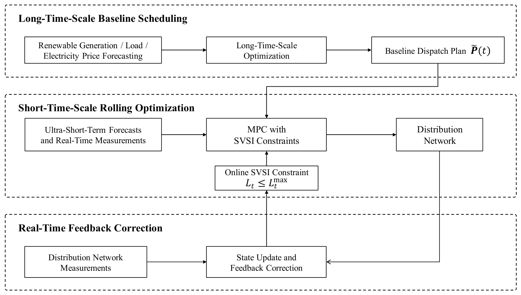
The multi-time-scale coordinated scheduling architecture considering the transmission–distribution boundary adopted in this paper consists of three layers: long-time-scale baseline scheduling, short-time-scale rolling optimization, and real-time feedback correction. Long-time-scale scheduling forms a baseline dispatch plan for a future operating period based on forecast information over a relatively long horizon, including renewable generation output, load demand, electricity prices, and transmission–distribution boundary exchange power. Short-time-scale rolling optimization takes the long-time-scale baseline schedule as a reference and incorporates the latest ultra-short-term forecast information to correct the outputs of controllable distributed generators, energy storage systems, flexible loads, and other distribution-side resources, as well as the deviation in transmission–distribution boundary exchange power. Real-time feedback correction updates the initial state of the next optimization cycle using actual measurements at the current sampling instant, thereby transforming the scheduling process from open-loop plan-based control into closed-loop rolling control.
Long-time-scale scheduling mainly plays the role of global planning. Its optimization objective can be formulated as the minimization of operating cost, considering the power purchasing cost from the main grid, flexible load scheduling cost, energy storage operating cost, and controllable distributed generation scheduling cost. The objective function can be expressed as:  C l o a d , i t
m i n F = m i n t = 1 T l ( C g r i d t P g r i d t + i = 1 m C l o a d , i t + j = 1 N S C s t a r , j t + k = 1 N G C D G t )
where T l is the optimization horizon of the long-time-scale scheduling; m , N S , and N G denote the numbers of flexible loads, energy storage systems, and controllable distributed generators, respectively; C g r i d t is the time-of-use electricity price of the main grid; P g r i d t is the active power exchanged between the distribution network and the upstream grid; and, C s t a r , j t , and C D G t represent the scheduling costs of flexible loads, energy storage systems, and controllable distributed generators, respectively.
The long-time-scale optimization result is not fixed and executed throughout the entire operating horizon. Instead, it serves as the reference trajectory for the short-time-scale MPC-based rolling optimization. The baseline dispatch plan can be written as:
P ˜ t = P ˜ g r i d t , P ˜ l o a d t , P ˜ s t a r t , P ˜ D G t T
where P ˜ g r i d t , P ˜ l o a d t , P ˜ s t a r t , P ˜ D G t denote the baseline values of tie-line exchange power, flexible load adjustment, energy storage charging/discharging power, and controllable distributed generation output, respectively.
Under this coordinated architecture, long-time-scale scheduling generates an economically optimized baseline dispatch plan based on forecast information on renewable generation, load demand, and electricity prices. Short-time-scale MPC takes this baseline plan as a reference and performs rolling corrections of adjustable resources by incorporating ultra-short-term forecast information and real-time measurement results. Meanwhile, the static voltage stability index (SVSI), obtained through online calculation based on local network equivalencing, is introduced into the short-time-scale MPC rolling optimization process as a static voltage stability constraint. The real-time feedback correction stage updates the initial conditions for the next optimization cycle according to the actual operating state of the distribution network, thereby forming a closed-loop coordinated scheduling framework that simultaneously considers economic operation, renewable energy accommodation capability, and static voltage security margin. The overall multi-time-scale coordinated scheduling framework is illustrated in Figure 1.

2.3. MPC-Based Rolling Optimization and Feedback Correction Process

In the short-time-scale rolling optimization stage, MPC uses rolling forecasts of intermittent distributed generation and load as input variables, takes the current real-time measurements of the system as the initial optimization state, and uses the long-time-scale baseline dispatch plan as the reference trajectory. On this basis, the control variables over a future finite horizon are solved in a rolling manner.
Let P o k denote the initial active power output of adjustable resources at the current sampling instant k , which is obtained from real-time measurements. Let Δ u k + t k denote the active power output increment predicted at time k for the future interval k + t 1 , k + t . Then, the short-time-scale rolling prediction model can be expressed as:
P k + i k = P o k + t = 1 i Δ u k + t k ,     i = 1 , 2 , , N
where P k + i k denotes the active power output predicted at time k for the future instant k + i , and N is the prediction horizon. This equation indicates that the predicted output at a future instant is jointly determined by the current measured initial value and the future control increments.
Taking the baseline dispatch plan issued by the long-time-scale optimization as the reference, the objective of the short-time-scale MPC optimization is to minimize the deviation between the predicted output and the reference output. Substituting Equation (4) into the MPC rolling optimization objective yields:
m i n J k = i = 1 N P o k + t = 1 i Δ u ( k + t | k ) P ˜ k + i Q 2
where P ˜ k + i is the reference output obtained from the long-time-scale optimization at time k + i , and Q is a weighting matrix used to characterize the importance of the deviation between the predicted output and the reference output. By solving Equation (5), the active power output increment sequence over the future control horizon can be obtained.
In practical implementation, MPC only applies the first control action in the optimized control sequence. Therefore, the active power output of adjustable resources at time k + 1 is given by
P T k + i k = P o k + Δ u T k + t k
When the system reaches time k + 1 , the actual active power output is obtained through the measurement system and is used as the initial value for the next rolling optimization cycle:
P o k + 1 = P r e a l k + 1
where P r e a l k + 1 denotes the actual active power output measured at time k + 1 after the control command is implemented, and P o k + 1 denotes the initial state for the next rolling optimization cycle. Through the feedback correction process described by Equation (7), MPC can continuously use real-time operating data to correct prediction deviations, allowing the scheduling results to be dynamically updated according to changes in the system state.
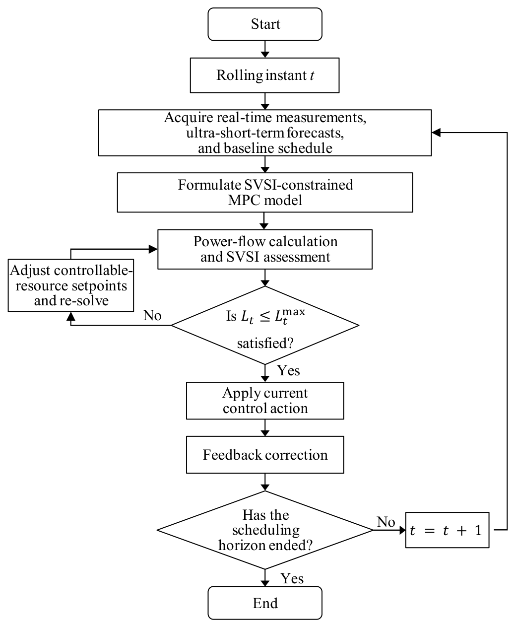
Through the mechanisms of rolling prediction, rolling optimization, and feedback correction, the short-time-scale MPC solves the future control sequence at each sampling instant based on ultra-short-term forecasts, the long-time-scale baseline dispatch plan, and the current real-time measurements. It then implements only the first control action and updates the initial state of the next optimization cycle using the measurements collected at the following sampling instant, thereby forming a closed-loop rolling control process.

3. SVSI Calculation Method Based on Local Network Equivalencing

3.1. Fast Online Assessment Method for the Stability Boundary

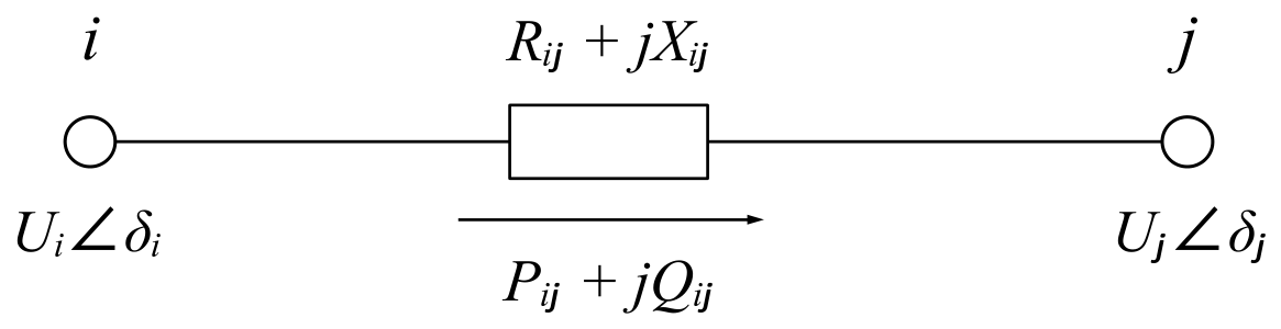
For a radial distribution network with multiple nodes, based on the current operating state, any transmission line can be equivalently represented by a line model consisting of an upstream node i, a downstream node j, and the branch impedance R i j + j X i j . To facilitate the derivation of the nodal static voltage stability index, this paper adopts the line model shown in Figure 2 to describe the voltage, power, and impedance relationships between node i and node j.
In Figure 2, U i δ i and U j δ j are the voltage phasors of node i and node j , respectively; R i j and X i j are the resistance and reactance of the branch, respectively; and P i j and Q i j are the active and reactive power flowing through branch i j into node j, respectively. Based on this line model and the existence condition of the power-flow solution, the static voltage stability index of node j can be obtained as:
L j = 4 [ P i j X i j Q i j R i j ) 2 + P i j R i j + Q i j X i j U i 2 U i 4
As shown in Equation (8), the nodal static voltage stability index is jointly affected by branch transmission power, line impedance, and the voltage magnitude of the upstream node. When the branch transmission power increases, the line voltage drop becomes more severe, or the nodal voltage level decreases, and L j increases accordingly, indicating that the operating state of the node is gradually approaching the static voltage stability boundary.
To evaluate the static voltage stability level on the distribution-network side under coordinated transmission–distribution operation, the maximum SVSI among all nodes in the distribution network is adopted as the system-level static voltage stability index:
L = max L j
Since this index takes the maximum value among all nodes, it can reflect the voltage stability condition of the weakest node in the system. When L is small, all nodes in the system are relatively far from the voltage stability boundary. When L approaches the allowable upper limit, at least one node in the system has an insufficient voltage stability margin, and corresponding control measures should be taken during the scheduling process.
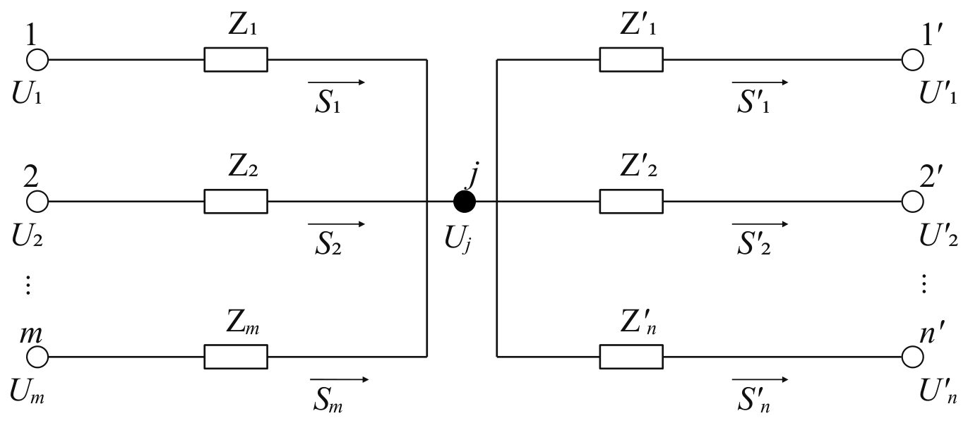
In conventional distribution networks with unidirectional power flow, Equation (8) can be directly used to calculate the static voltage stability index of each node. However, after the integration of high-penetration distributed generation, the power-flow direction of some branches may change, and multiple power-inflow branches and multiple power-outflow branches may coexist around a node. In this case, directly calculating the SVSI based on a single-branch model may fail to accurately represent the equivalent electrical relationship of the local network around the node. Therefore, this paper introduces a local network equivalencing method, in which multiple inflow branches and outflow branches around a node are equivalently represented by equivalent branches. The local network model of the distribution network is shown in Figure 3.
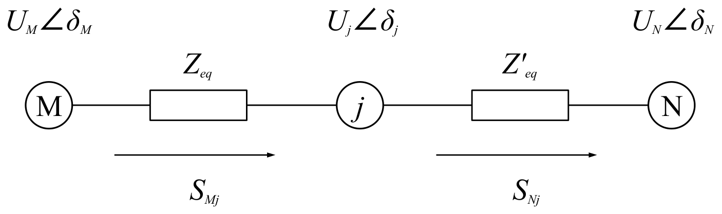
Based on the current power-flow results, the branches connecting nodes 1 , 2 , , m to node j inject power into node j, while node j may also export power through other branches. Suppose that there are m branches through which power flows into node j, and n branches through which power flows out of node j. Let U 1 , U 2 , , U m be the voltages of neighboring nodes on the inflow side, Z 1 , Z 2 , , Z m be the impedances of the inflow-side branches, and S 1 , S 2 , , S m be the corresponding branch transmission powers. By equivalently processing the local network shown in Figure 3, the complex multi-branch connection relationship can be transformed into the local network equivalent model shown in Figure 4.
In Figure 4, M and N are the equivalent nodes on the inflow side and outflow side, respectively; U M and U N are the voltages of the equivalent nodes; and Z e q and Z e q are the equivalent impedances on the inflow side and outflow side, respectively. They are the reciprocals of the equivalent branch admittances Y e q and Y e q . Through this equivalent model, multiple inflow branches and multiple outflow branches can be equivalently represented by two equivalent branches, thereby providing a unified local network representation for SVSI calculation under bidirectional power-flow variations.
For multiple branches flowing into node j, the equivalent admittance and equivalent node voltage on the inflow side are given by:
Y e q = i = 1 m Y i
U M = i = 1 m Y i U i Y e q
where Y i = 1 / Z i . Equations (10) and (11) indicate that the local equivalencing of the inflow side combines multiple inflow branches according to their admittance relationships, thereby maintaining the consistency of the local power transmission relationship at node j before and after equivalencing.
Similarly, for multiple branches through which node j exports power to other nodes, the equivalent admittance and equivalent node voltage on the outflow side are expressed as:
Y e q = i = 1 n Y i
U N = i = 1 n Y i U i Y e q
where n is the total number of branches through which power flows out of node j. Through Equations (10)–(13), the multi-branch local network around node j can be equivalently represented by the two-sided equivalent network shown in Figure 4, thereby reducing the difficulty of SVSI calculation under complex power-flow relationships.
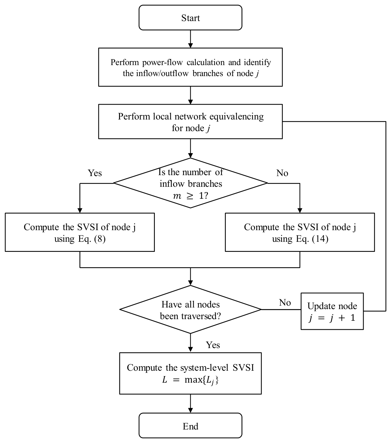
After local network equivalencing is completed, the corresponding stability index calculation method should be selected according to the number of branches m through which power flows into node j. When m 1 , at least one branch delivers power to node j. In this case, the SVSI of node j is calculated using Equation (8), where the corresponding voltage, impedance, and power variables are substituted by the quantities obtained from the local equivalent network.
When m = 0 , there is no power-inflow branch around node j, and node j only exports power to external branches. In this case, the conventional inflow-branch model corresponding to Equation (8) is no longer applicable. The nodal stability index should instead be calculated according to the existence condition of the power-flow solution between node j and the outflow-side equivalent node N, which can be expressed as:
L j = 4 P N j X j N Q N j R j N 2 P N j R j N + Q N j X j N U N 2 U N 4
where R j N and X j N are the resistance and reactance of the equivalent branch between node j and the equivalent node N, respectively; P N j and Q N j are the active and reactive power flowing from node j to the equivalent node N, respectively; and U N is the voltage magnitude of the equivalent node N. Equation (14) is used to handle the special case in which node j has no power-inflow branch, enabling the SVSI calculation to cover reverse power-flow scenarios that may occur after the integration of high-penetration distributed generation.
Based on the above calculation procedure, the online SVSI calculation process based on local network equivalencing is shown in Figure 5.

3.2. Rolling Correction Mechanism for the Stability Boundary

Let the rolling optimization time be denoted by t. After power-flow calculation is performed according to the current operating state, the static voltage stability index of each node can be obtained using the local network equivalencing method described in Section 3.1. Then, the overall voltage stability index L t of the distribution network at the current time can be obtained using Equation (9). To ensure that the operating point of the distribution network does not exceed the allowable static voltage stability boundary, the static voltage stability constraint is expressed as:
0 < L t L t max
where L t is the voltage stability index of the distribution network at time t, and L t max is the allowable upper limit of the voltage stability index at time t, which can be specified by the system operator according to actual operating requirements.
Equation (15) represents the static voltage stability requirement for a single operating point. In the MPC framework, this constraint is further extended to each step of the prediction horizon, as described in Section 4.2.2. At each rolling instant, the current operating state is updated using real-time measurements and ultra-short-term forecasts, and the SVSI constraint is incorporated directly into the subsequent MPC optimization.
As illustrated in Figure 6, for each candidate control sequence generated during the MPC optimization, the corresponding predicted power-flow states are calculated over the prediction horizon. Based on the predicted power-flow directions, the local equivalent network of each node is reconstructed and the nodal SVSI values are evaluated. The candidate control sequence is regarded as feasible only when the system-level SVSI satisfies the prescribed upper limit throughout the prediction horizon. The optimizer then determines the optimal feasible control sequence, of which only the first control action is implemented. At the next rolling instant, the measured operating state is fed back and the above procedure is repeated. In this way, the SVSI is directly coupled with the MPC feasibility evaluation and optimization process rather than being used only as an external post-optimization check.

4. MPC-Based Multi-Time-Scale Coordinated Scheduling Model for Distribution Networks

With the large-scale integration of distributed generation, power interactions between transmission and distribution networks have become increasingly coupled, which imposes new requirements on rolling optimization on the distribution-network side and coordinated operation at the transmission–distribution interface. Due to the large number of distributed generation nodes in distribution networks and the heavy communication burden, it is difficult to achieve real-time response to photovoltaic and wind power fluctuations across the system. Therefore, this paper proposes a multi-time-scale coordinated optimal scheduling method. At the long time scale, with a 15-min scheduling interval, an optimal power flow problem is solved with economic optimality as the objective function, and the scheduling plan for the next 1 h is obtained. At the short time scale, based on the principle of model predictive control, the ultra-short-term rolling forecasts of wind and photovoltaic power are used as references. The short-time-scale optimization is activated every 5 min, takes the long-time-scale scheduling results as reference values, and on a rolling basis, calculates the active power output increments over the next 15 min. However, only the control command of the first time interval is executed each time. In this way, the active power outputs of controllable distributed generators are corrected in a timely manner, thereby maximizing the accommodation of intermittent renewable energy.

4.1. Long-Time-Scale Optimization Scheduling

At the long time scale, an economic scheduling model is adopted for the active power optimal scheduling of the active distribution network, with the objective of minimizing the scheduling cost, as follows:
min F = min t = 1 T 1 ( c grid ( t ) P grid ( t ) + i = 1 m C load i ( t ) + j = 1 N S C stor j ( t ) + k = 1 N G C DG ( t ) )
where T1 denotes the long-time-scale optimal scheduling period; m, NS, and NG denote the numbers of flexible loads, energy storage devices, and controllable distributed generators, respectively; c grid ( t ) denotes the time-of-use electricity price of the grid; P grid ( t ) denotes the active power of the tie line connected to the main grid; C load i ( t ) denotes the scheduling cost of flexible loads; C stor j ( t ) denotes the scheduling cost of batteries; and C DG ( t ) denotes the scheduling cost of controllable distributed generators. The specific mathematical models of the scheduling costs are given as follows:
(1)
Flexible load scheduling cost.
The relationship between the flexible load scheduling cost and the power variation is expressed as follows:
C load i ( t ) = 1 α i Δ P load i 2 ( t ) + β i 2 P load i 0 ( t ) α i Δ P load i ( t )
where α i and β i bare the scheduling cost coefficients of flexible loads, respectively; P load i 0 is the initial active power of the flexible load before scheduling; and Δ P load i is the power variation in the flexible load.
(2)
Scheduling cost of battery energy storage.
The battery energy storage system operates in either the charging or discharging state. Both charging and discharging affect the service life of the battery. Therefore, the virtual scheduling cost of the battery energy storage system is assumed as follows:
C stor j ( t ) = λ ess P stor j 2 ( t )
where λ ess denotes the scheduling cost coefficient of the battery energy storage system, and P stor j ( t ) denotes the charging/discharging power of the battery energy storage system.
(3)
Scheduling cost of controllable distributed generators.
C DG k ( t ) = a k P DG k 2 ( t ) + b k P DG k ( t ) + c k
where a k , b k , and c k denote the scheduling cost coefficients of controllable distributed generators, respectively; and P DG k ( t ) denotes the active power output of controllable distributed generators.

4.2. Short-Time-Scale Optimization Scheduling

Traditional optimal scheduling control in power systems adopts an open-loop manner. Specifically, the optimal solution over a future optimization horizon is obtained at the initial stage of optimization and then issued at one time. When the load forecasting accuracy is high, this scheduling mode can satisfy practical scheduling requirements. However, active distribution networks contain a large number of intermittent renewable distributed generators, whose forecasting accuracy is much lower than that of load forecasting. Moreover, the forecasting accuracy decreases as the prediction time scale increases. Therefore, the optimal scheduling results obtained by taking such forecasts as input variables cannot be directly applied to the actual system. It is necessary to adopt an MPC-based rolling-horizon optimization scheduling strategy with feedback correction.
MPC takes the rolling forecasts of intermittent renewable distributed generators as input variables, uses the actual measured values of controllable distributed generators in the active distribution network as the initial value P0(k), and takes the active power output increments of distributed generators over a finite future horizon as control variables to perform rolling optimization over the finite future horizon.

4.2.1. Rolling Forecasting Model

By solving the control variables through rolling optimization, the active power outputs of distributed generators, energy storage systems, and flexible loads over the future finite horizon are predicted. The prediction model is formulated as follows:
P ( k + i | k ) = P 0 ( k ) + t = 1 i Δ u ( k + t | k ) ,           i = 1 , 2 , , N
where Po(k) denotes the initial active power output of controllable distributed generators, energy storage systems, and flexible loads, which is obtained from actual measurements; Δ u ( k + t | k ) denotes the predicted active power output increment over the interval [k + (t − 1), k + t] at time k, which is the control variable to be optimized; P(k + i|k) denotes the active power output at future time k + i predicted at time k; and N denotes the prediction horizon.

4.2.2. Objective Function for Optimization

Taking the active power output dispatched at the long time scale as the reference value, the short-time-scale optimization aims to minimize the correction deviation of active power output. Therefore, the quadratic performance index for short-time-scale active power optimal scheduling based on model predictive control is established as follows:
min J ( k ) = i = 1 N P ( k + i k ) P ˜ ( k + i ) Q 2 = i = 1 N P 0 ( k ) + i = 1 i Δ u T ( k + t k ) P ˜ ( k + i ) Q 2
s . t .           P min ( k + i ) P 0 ( k ) + t = 1 i Δ u T k + t k P max k + i
s o c storj ( k + i k ) = s o c storj ( k + i 1 k ) ( 1 σ ) η P storj ( k + i k )
s o c min s o c ( k + i k ) s o c max
P ( k + i k ) = P ˜ Σ Load ( k + i k ) + P loss ( k + i k ) , i = 1 , 2 , N
where P ˜ ( k + i ) denotes the active power output reference value at time k + i .
  • In addition to the above operational constraints, the static voltage stability constraint in Equation (15) is explicitly incorporated into the MPC optimization over the prediction horizon. For each predicted time step k + i , the predicted operating state determined by the candidate control variables is used to perform power-flow calculation. According to the resulting power-flow directions, the local equivalent network of each node is reconstructed, and the corresponding nodal SVSI L ( k + i | k ) is calculated using the method described in Section 3.1. The system-level SVSI is then obtained as the maximum nodal value and constrained as
0 < L ( k + i | k ) = max j Ω L j ( k + i | k ) L m a x ,     i = 1,2 , , N
where L ( k + i | k ) denotes the predicted SVSI of node j at time k + i based on the information available at time k , and L m a x denotes the allowable upper limit of the system-level SVSI. During the sequential quadratic programming process, this constraint is evaluated together with the predicted power-flow state for each candidate control sequence. Therefore, changes in power-flow direction caused by the control-variable updates are reflected in the local network equivalencing and SVSI calculation, allowing the voltage-stability boundary to participate directly in the MPC optimization rather than being evaluated only after the optimization.
P ˜ ( k + i ) = [ P ˜ grid ( k + i ) , Δ P ˜ load T ( k + i ) , P ˜ stor T ( k + i ) , P ˜ DG T ( k + i ) ] T
where P ( k + i k ) denotes the active power output of each controllable distributed generator at future time k + i predicted at time k, which is specifically expressed as follows:
P ( k + i k ) = [ P grid ( k + i k ) , Δ P load T ( k + i k ) , P stor T ( k + i k ) , P DG T ( k + i k ) ] T
where s o c ( k + i k ) denotes the state of charge of the battery energy storage system at future time k + i predicted at time k; s o c min and s o c max denote the lower and upper limits of the state of charge, respectively; P ˜ Σ Load ( k + i k ) denotes the net load at future time k + i predicted at time k; and P loss ( k + i k ) denotes the system active power loss at future time k + i predicted at time k.
  • Where Δ u T k + i k denotes the column vector of active power output variations in controllable distributed generators at future time k + i predicted at time k. The active power variations over the future N time instants are optimized and solved using the sequential quadratic programming method as follows:
{ Δ u T ( k + 1 k ) , Δ u T ( k + 2 k ) , , Δ u T ( k + N k ) }
The first control-variable column vector in the control sequence is issued, and the active power outputs of controllable distributed generators, energy storage systems, and flexible loads in the active distribution network at time k + 1 are obtained as follows:
P ( k + 1 k ) = P 0 ( k ) + Δ u T ( k + 1 k )

4.2.3. Feedback Correction

Under the current forecasting accuracy of wind and photovoltaic power, the predictive MPC control cannot guarantee that the actual wind and photovoltaic outputs are identical to their forecasted values. This may lead to deviations between the advance-dispatched outputs of controllable distributed generators and the actual active power outputs. Therefore, a feedback correction process is required. The current actual active power output of the system is used as the initial value for the next round of rolling optimal scheduling, thereby forming a closed-loop control structure. This process mitigates the uncertainties of the system, wind power, and photovoltaic power, and makes the predicted active power outputs in the next round more consistent with the actual values and more accurate, namely:
P 0 ( k + 1 ) = P real ( k + 1 )
where Preal(k + 1) denotes the actual active power output at time k + 1 collected by the measurement system after the active power output predicted at time k is dispatched; and P0(k + 1) denotes the initial active power output at time k + 1.

4.3. Transmission–Distribution Boundary Coordination Constraints

On the basis of the above distribution-network-side rolling optimization model, transmission–distribution boundary coordination constraints are further introduced to coordinate the scheduling results on the distribution network side with the power interaction requirements of the main grid. The transmission network and the distribution network exchange power through points of common coupling, and the boundary interaction relationship can be expressed as
P b , t T = P b , t T D
P b , t D = P b , t T D
where P b , t T denotes the active power exchanged between the transmission-network side and the b -th boundary node at time t ; P b , t D denotes the active power exchanged between the b -th boundary node and the distribution-network side at time t ; and P b , t T D denotes the active power exchanged between the transmission and distribution networks at the b -th boundary node. The direction from the transmission network to the distribution network is defined as positive. The above constraints ensure that the power exchange between the transmission-network side and the distribution-network side remains consistent at the point of common coupling.
Considering the capacity limit of the transmission–distribution boundary channel, the boundary exchange power should satisfy
P ¯ b T D P b , t T D P ¯ b T D
where P ¯ b T D is the maximum allowable transmission power of the b -th transmission–distribution boundary. This constraint is used to ensure that the power exchange at the transmission–distribution boundary does not exceed the capacity of the boundary channel.
When the system contains multiple transmission–distribution boundaries, the above constraints should hold simultaneously for all boundary nodes and scheduling periods, namely,
b Ω T D , t Ω T
where Ω T D is the set of transmission–distribution boundaries, and Ω T is the set of scheduling periods. Through the above boundary coordination constraints, the long-time-scale baseline scheduling results can be linked with the short-time-scale MPC-based rolling optimization process, so that the optimized results of adjustable resources on the distribution network side satisfy the power interaction requirements of the main grid.

5. Case Studies

5.1. Test System and Network Parameters

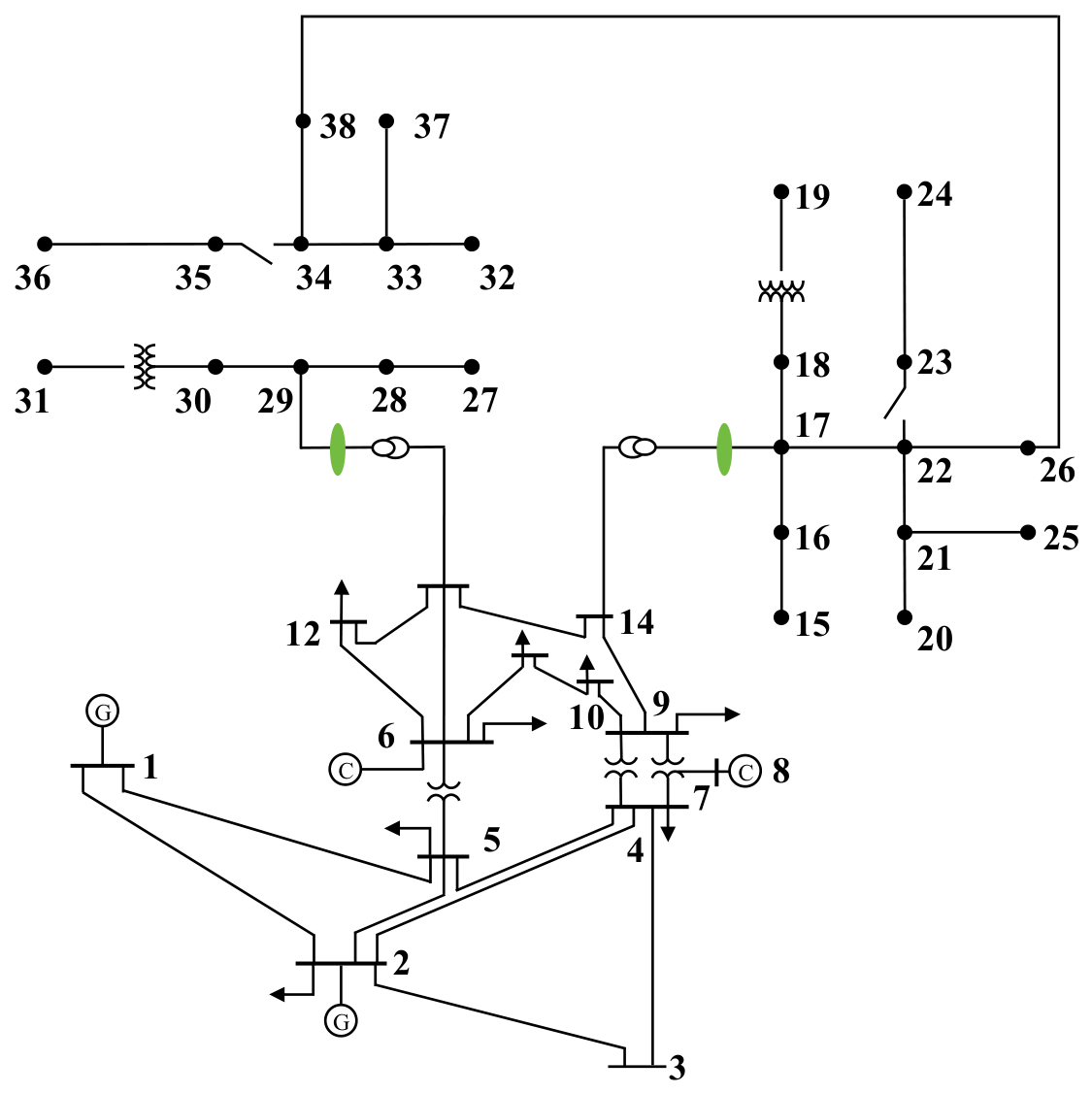
The simulation is conducted on a transmission–distribution coupled system consisting of the IEEE 14-bus transmission network and two modified IEEE 13-node distribution networks, as shown in Figure 7. The two distribution networks are connected to buses 13 and 14 of the IEEE 14-bus transmission network, respectively, and are interconnected through a tie line. The system base capacity is set to 10 MVA, the base voltage on the distribution side is 12.66 kV, and the allowable nodal voltage range is set to 0.95–1.05 p.u. The relevant parameter settings for the microturbines, flexible loads, and energy storage system are shown in the Table 1.
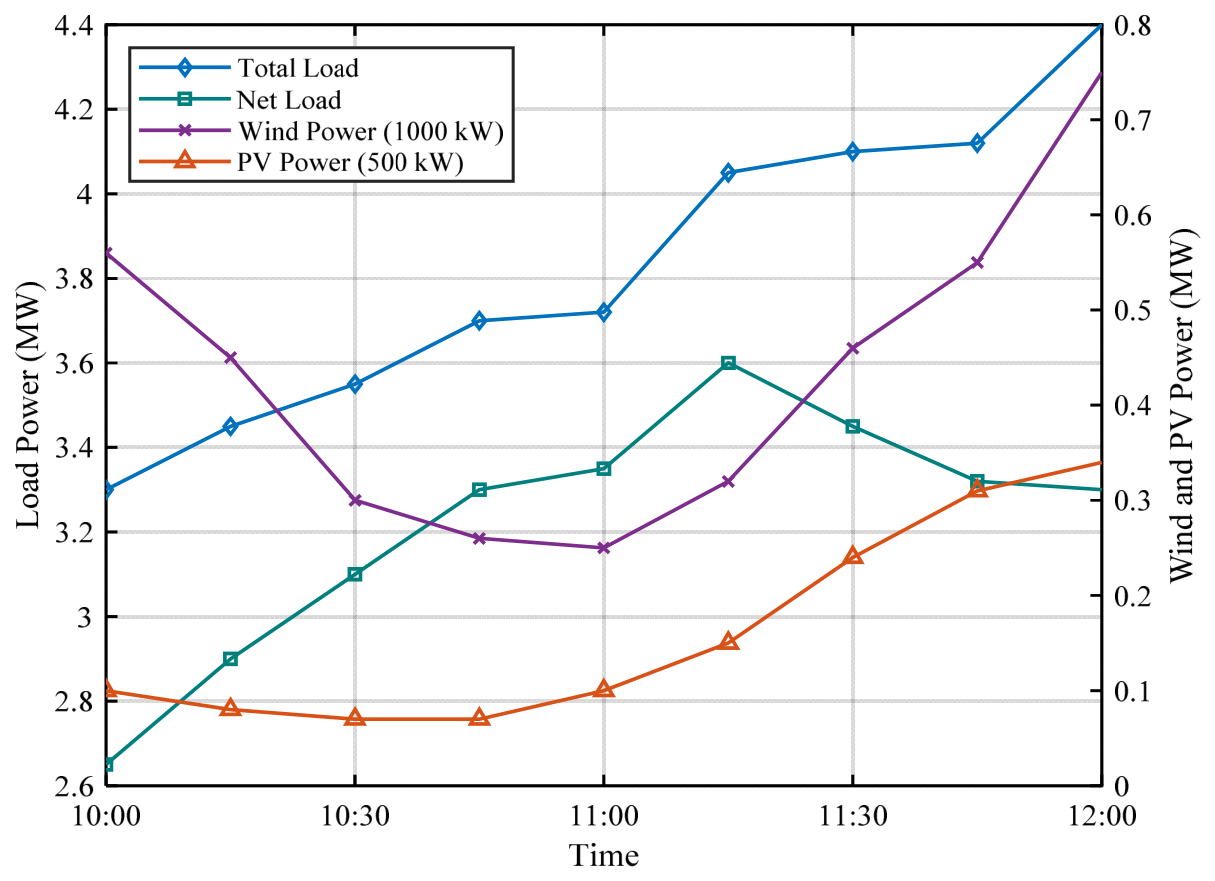
In the test system, the transmission network exchanges power with the distribution networks through transmission–distribution interface buses. On the distribution side, adjustable resources, including wind power, photovoltaic generation, energy storage systems, and flexible loads, are integrated. Two variation patterns of distributed generation are considered in the case studies: one represents a slow variation scenario of wind and photovoltaic outputs, and the other represents a fast fluctuation scenario of wind and photovoltaic outputs. According to the typical variation characteristics of wind power, photovoltaic generation, and load in active distribution networks, the corresponding active-power profiles are synthetically generated by manually specifying the power values at discrete time instants. The rated capacities of the wind power and photovoltaic units are set to 1000 kW and 500 kW, respectively. The operating profile for Case Study 1 is shown in Figure 8. At the long time scale, with a time interval of 15 min, a baseline dispatch plan for the outputs of adjustable resources in the distribution networks and the transmission–distribution interface exchange power is generated for the next 1 h. At the short time scale, MPC-based rolling optimization is activated every 5 min. The prediction horizon and control horizon are both set to three steps, i.e., M = N = 3, corresponding to a 15-min rolling optimization horizon. At each rolling instant, only the control instruction for the first 5-min interval is implemented, after which the optimization horizon is shifted forward for the next rolling optimization.

5.2. Case Study 1: Scenario Setting

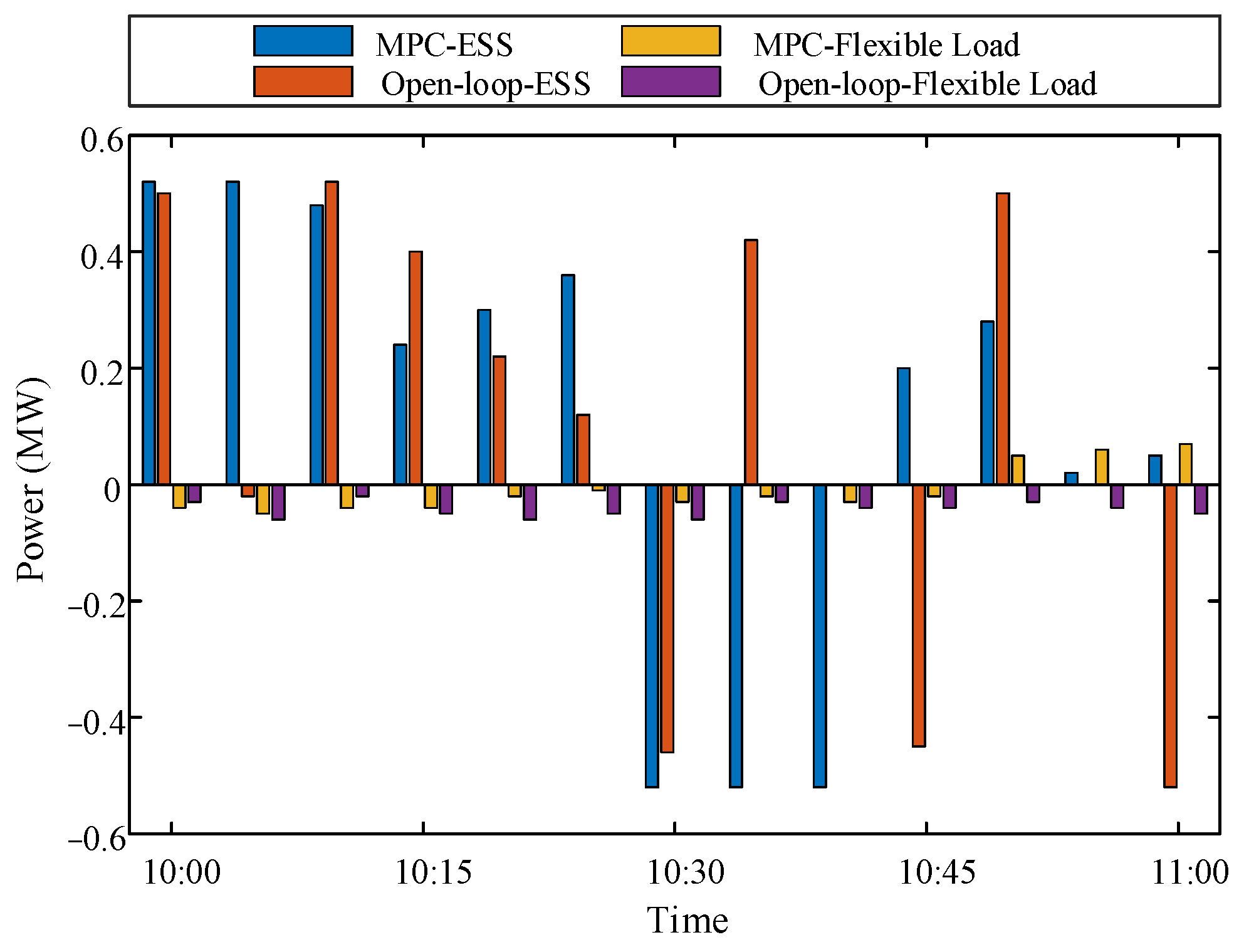
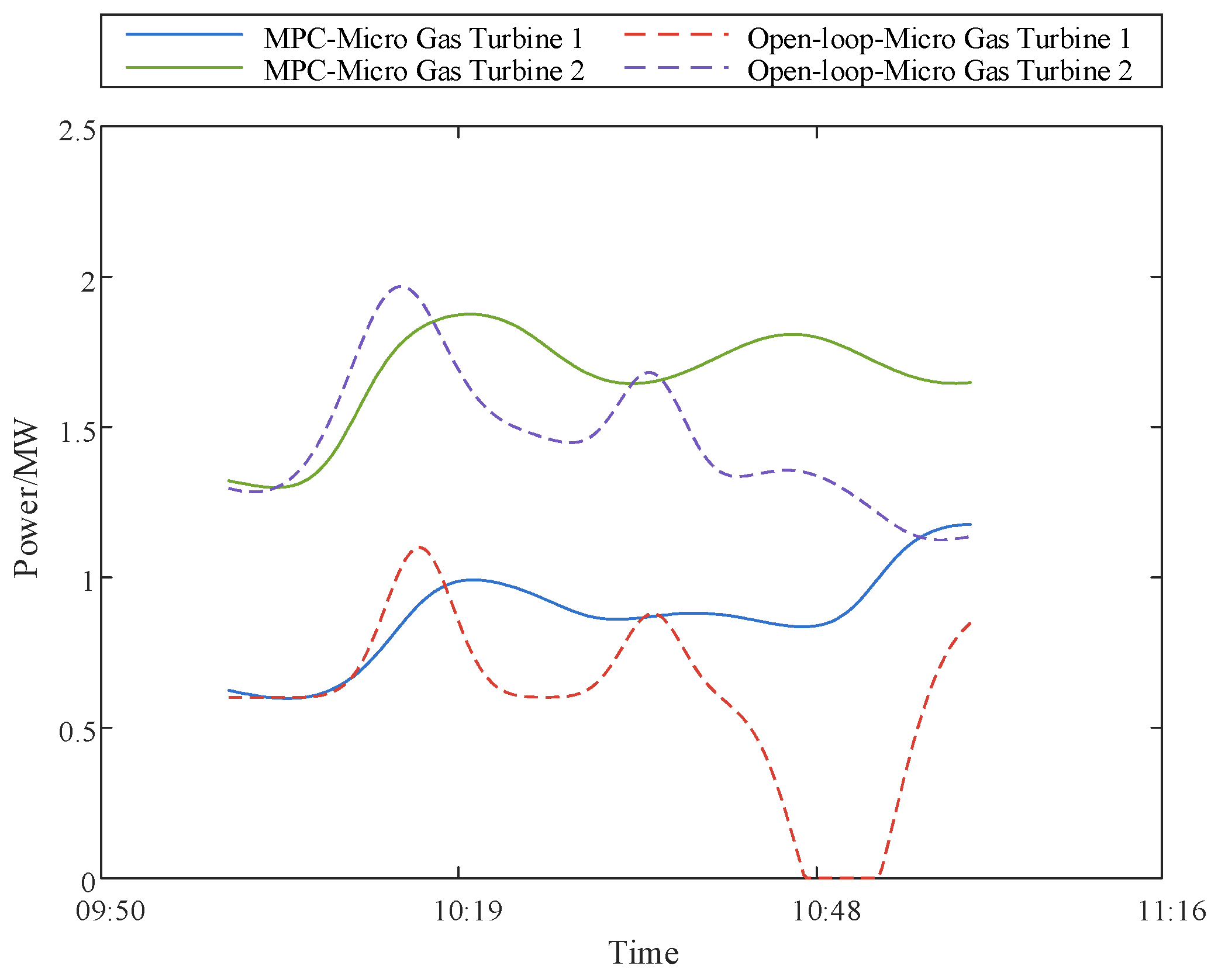
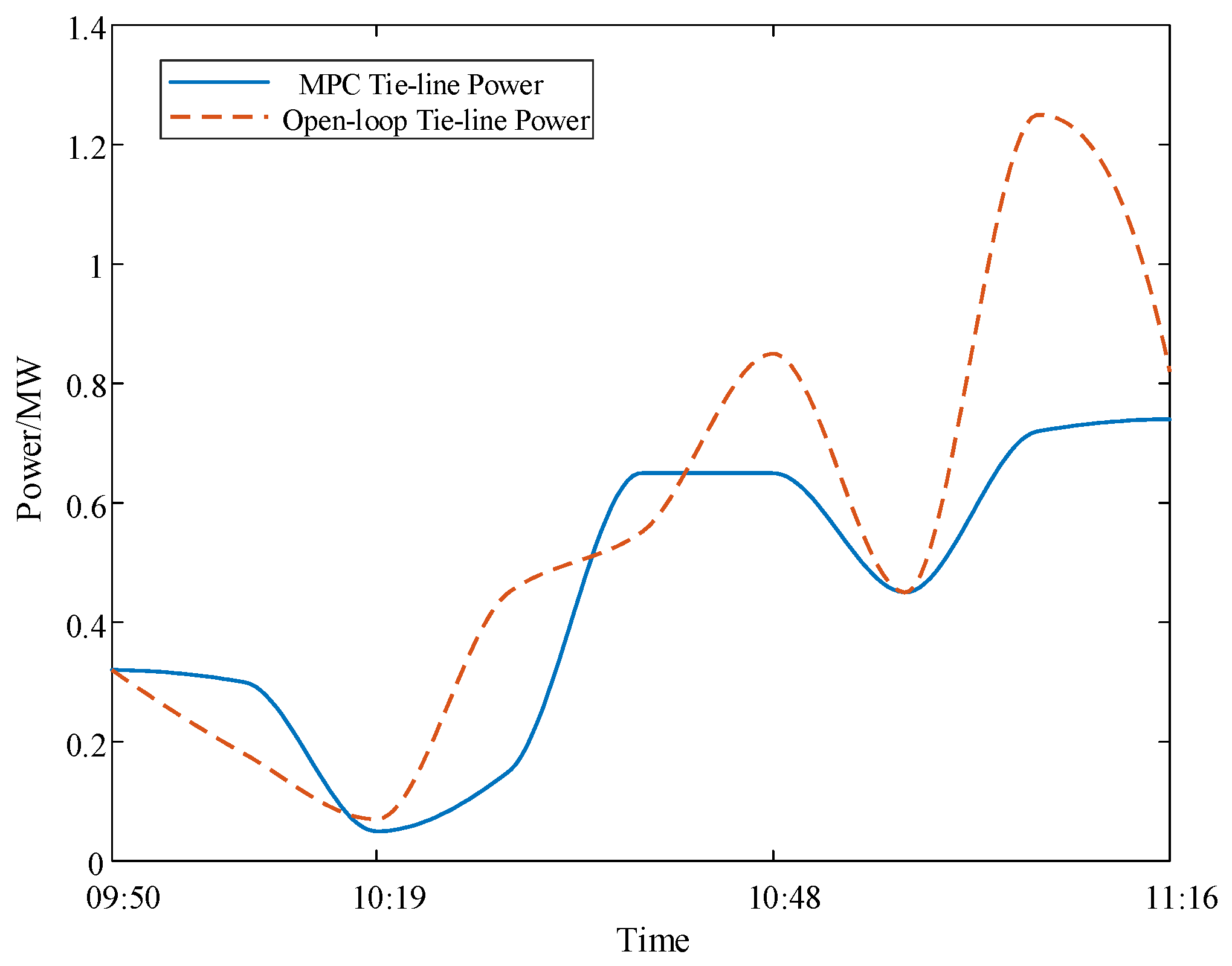
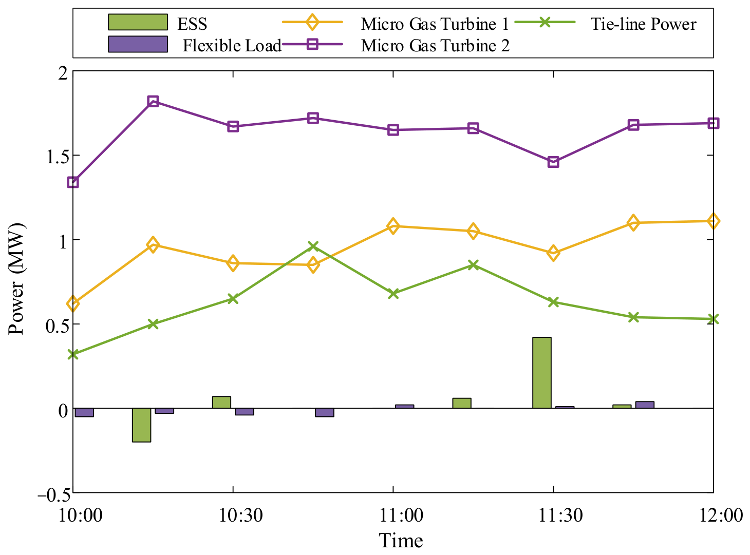
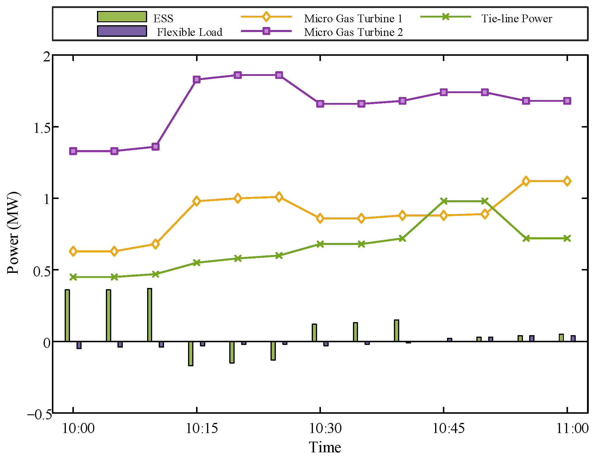
In the scenario of Case Study 1, the forecast data from 10:00 to 12:00 are taken as an example to perform long-time-scale optimal scheduling, as shown in Figure 8. Figure 9 shows the scheduled active power outputs of each controllable distributed generator at the long time scale. Figure 10 shows the active power outputs of each controllable distributed generator at the short time scale. In traditional open-loop optimal scheduling, the load, wind power, and photovoltaic power outputs over the future optimization horizon are predicted at one time, and the corresponding optimization calculation is then performed to issue the scheduling plan. Figure 11 and Figure 12 compare the scheduling results obtained by traditional open-loop optimization and MPC-based optimal scheduling, respectively.
The simulation results show that the active power output trend issued by MPC-based rolling optimization control is consistent with that obtained by traditional open-loop optimal power flow calculation, and the optimization results are relatively close. However, compared with traditional open-loop optimal power flow-based active power scheduling, the MPC-based rolling optimization takes the active power output variation as the control variable and continuously uses the actual measured values of the system for feedback correction. Therefore, the MPC-based rolling optimal scheduling results are smoother, which is more conducive to coping with the fluctuation and uncertainty of intermittent distributed generators. Meanwhile, it ensures smooth outputs of controllable distributed generators, reduces the mechanical wear of controllable distributed generators, and prolongs their service life.

5.3. Case Study 2: Scenario Setting

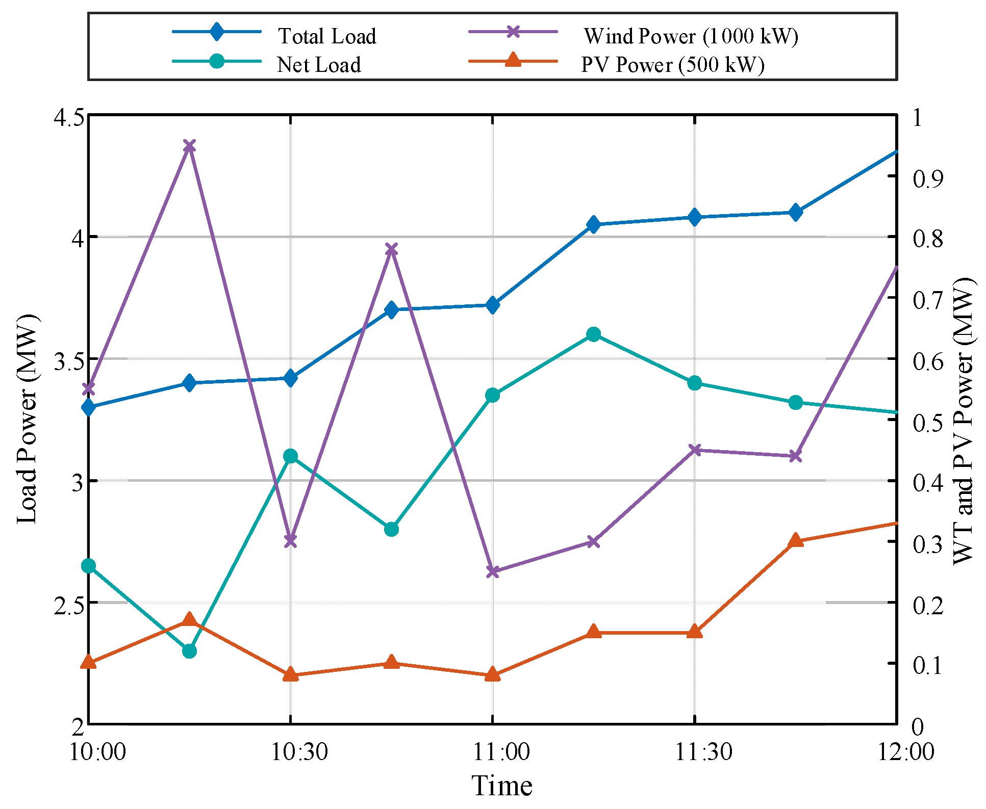
Figure 13 presents the forecast data of wind and photovoltaic power with rapid fluctuations from 10:00 to 12:00 in the scenario of Case Study 2. Figure 14, Figure 15 and Figure 16 compare the scheduling results of traditional open-loop optimal scheduling and MPC-based optimal scheduling under the scenario with rapid fluctuations in wind and photovoltaic active power outputs.
The simulation results of Case Study 2 show that, under rapid fluctuations in wind and photovoltaic power outputs, the active power outputs obtained by traditional open-loop optimal scheduling fluctuate significantly. In contrast, the MPC-based feedback rolling optimization control method is more effective than the traditional open-loop control method in accommodating wind power fluctuations and smoothing the active power outputs of distributed generators. By comparing the simulation results under different scenarios in Case Study 1 and Case Study 2, it can be observed that the MPC-based feedback rolling optimization control strategy exhibits superior performance in handling the fluctuations in intermittent energy sources.

5.4. Sensitivity Analysis

5.4.1. Performance Under Different Representative Operating Periods

To further evaluate the applicability of the proposed method under different daily operating conditions, representative operating periods corresponding to morning ramping, daytime operation, and evening peak conditions are considered. In addition to the original 10:00–12:00 cases, two additional operating periods, 06:00–08:00 and 18:00–20:00, are introduced. The morning period represents the simultaneous increase in load demand and photovoltaic generation, whereas the evening period represents the decrease in photovoltaic output accompanied by an increase in load demand. The original slow-variation and rapid-fluctuation cases during 10:00–12:00 are retained as representative daytime operating conditions. For all cases, the same network topology, control strategy, and MPC parameter settings are adopted. The maximum SVSI, minimum bus voltage, energy loss, renewable energy curtailment, and operating cost are used to evaluate the performance of the proposed method. The results are summarized in Table 2.
As shown in Table 2, the operating characteristics of the system vary significantly among the representative periods. During the morning ramping period, the simultaneous increase in load and photovoltaic generation results in a gradual redistribution of power flow. During the daytime period, the proposed method maintains satisfactory voltage-security performance under both slow and rapid renewable-generation variations. The evening peak period represents a more stressed operating condition because photovoltaic generation decreases while the load demand increases, resulting in a reduced voltage-security margin and increased dependence on controllable resources. Nevertheless, the proposed coordinated rolling optimization method maintains the SVSI and bus voltages within their allowable limits over all considered operating periods. These results further demonstrate the adaptability of the proposed method to different daily operating conditions.

5.4.2. Performance Under Different Renewable Energy Penetration Levels

To further evaluate the applicability of the proposed method under different renewable energy integration levels, the installed capacities of wind power and photovoltaic generation are proportionally adjusted while keeping the load level, network topology, and temporal variation patterns of renewable generation unchanged. The original case with 1000 kW wind power and 500 kW photovoltaic generation is taken as the base case, and renewable energy penetration levels of 80%, 100%, 120%, and 140% are considered. The corresponding operating results are summarized in Table 3.
As shown in Table 3, increasing the renewable energy penetration level generally reduces the system operating cost due to the increased utilization of renewable generation. Meanwhile, the maximum SVSI gradually increases and the minimum bus voltage decreases slightly as the renewable energy penetration level rises, indicating a stronger impact of high renewable integration on the system voltage-security margin. In addition, renewable energy curtailment becomes more evident at higher penetration levels. Nevertheless, the proposed coordinated rolling optimization method maintains the SVSI and bus voltages within their allowable limits under all considered penetration levels, demonstrating its adaptability to different renewable energy integration conditions.

5.4.3. Sensitivity Analysis of MPC Parameter Settings

To further justify the selection of the MPC parameters, a sensitivity analysis is conducted with respect to the control interval, prediction horizon, control/prediction steps, and weighting settings. The original parameter configuration, i.e., a 5-min control interval, a 15-min rolling optimization horizon, and M = N = 3, is taken as the baseline case. Other parameter combinations are then tested while keeping the network topology, load level, renewable generation profiles, and other system parameters unchanged. The effects of different MPC parameter settings are evaluated in terms of the maximum SVSI, minimum bus voltage, operating cost, renewable energy utilization, and computation time. The corresponding results are summarized in Table 4.
As shown in Table 4, extending the prediction horizon from 10 min to 15 min improves the voltage-security performance, as reflected by the reduced maximum SVSI and increased minimum bus voltage. Meanwhile, the operating cost is reduced and renewable energy utilization is slightly improved. When the prediction horizon is further extended to 20 min, only marginal performance improvement is obtained, whereas the computation time increases noticeably. In contrast, increasing the control interval reduces the updating frequency of the rolling optimization and weakens the ability of the controller to respond rapidly to renewable power variations, resulting in a higher maximum SVSI and a lower minimum bus voltage.
The results under different weighting settings further indicate that increasing the emphasis on security-related tracking performance can improve the voltage-security margin, but may lead to a moderate increase in operating cost. Overall, the parameter combination of a 5-min control interval, a 15-min prediction horizon, and M = N = 3 provides a favorable compromise among voltage stability, economic performance, renewable energy utilization, and computational efficiency. Therefore, this parameter configuration is adopted in the subsequent case studies.
To further assess the real-time applicability of the proposed MPC framework, all simulations were implemented in MATLAB R2025b on a 64-bit Windows 11 computer equipped with an Intel Core i7-13700H processor and 32 GB RAM. The nonlinear rolling optimization problem was solved using the sequential quadratic programming method. The computation time reported in Table 4 represents the average wall-clock time required for one complete rolling optimization step. Under the adopted baseline setting of a 5-min control interval, a 15-min prediction horizon, and M = N = 3 , the average computation time is 0.84 s. Among all parameter configurations considered in Table 4, the largest average computation time is 1.19 s, corresponding to approximately 0.40% of the shortest control interval of 300 s. Therefore, the proposed method provides sufficient computational margin for online rolling implementation.
The numerical results also demonstrate the adaptability of the proposed framework to time-varying operating conditions. As shown in Table 2 and Table 3, the prescribed SVSI and bus-voltage limits are maintained under different representative operating periods, rapid renewable-generation fluctuations, and renewable-energy penetration levels ranging from 80% to 140%. Unlike robust optimization, which generally seeks solutions that remain feasible within a predefined uncertainty set, and distributionally robust optimization, which considers an ambiguity set of probability distributions [37,38], the proposed MPC framework addresses forecast deviations through receding-horizon re-optimization and explicit measurement feedback. At each rolling instant, updated forecasts and measurements are incorporated, only the first optimized control action is implemented, and the measured state is used to initialize the next optimization cycle. The operating-state-dependent SVSI constraint is updated accordingly. Therefore, the specific advantage of the proposed framework for the problem considered here lies in its ability to adapt the optimization and corrective actions to updated operating information, rather than in claiming universal numerical superiority over robust optimization methods.

5.5. Static Voltage Stability Analysis

5.5.1. SVSI-Based Static Voltage Stability Analysis

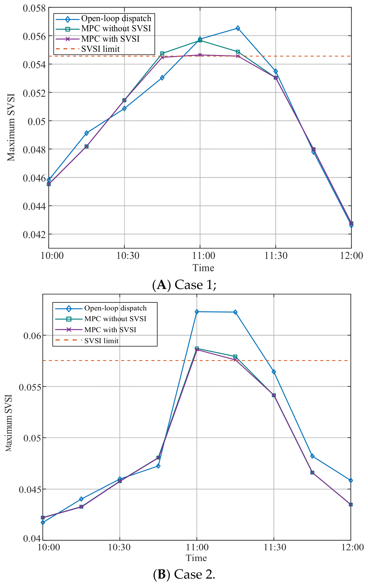
To further verify the effectiveness of the proposed method in improving the static voltage stability of the distribution network, the nodal static voltage stability index was calculated at each time instant based on Case 1 and Case 2. The maximum SVSI among all nodes in the entire network was then selected as the system-level evaluation index for static voltage stability. A larger SVSI indicates that the system operating point is closer to the static voltage stability boundary, whereas a smaller SVSI represents a more sufficient static voltage stability margin. Three scheduling methods were compared in this study: conventional open-loop dispatch, MPC dispatch without SVSI constraints, and MPC dispatch with SVSI constraints. The results are shown in Figure 17 and Table 5.
Figure 17A shows the variation curves of the system maximum SVSI under different scheduling methods in Case 1, where wind power and photovoltaic output vary slowly. It can be observed that, with variations in renewable generation and load levels, the SVSI values of conventional open-loop dispatch and MPC dispatch without SVSI constraints increase significantly during certain periods, indicating that the system operating point gradually approaches the static voltage stability boundary. In particular, conventional open-loop dispatch results in a relatively high maximum SVSI during high-risk periods because it lacks a rolling correction mechanism. Although MPC dispatch without SVSI constraints can correct forecasting deviations based on real-time measurement information, the SVSI may still approach or exceed the allowable upper limit. By contrast, the proposed MPC rolling optimization method with SVSI constraints can adjust the control variables in a timely manner when the system maximum SVSI approaches its limit, thereby maintaining the system operating point within the allowable range of static voltage stability.
Figure 17B shows the variation curves of the system maximum SVSI under different scheduling methods in Case 2, where wind power and photovoltaic output change abruptly. As shown in the figure, when renewable generation undergoes sudden changes, the system power-flow distribution varies rapidly. Under conventional open-loop dispatch, the system maximum SVSI increases significantly and exceeds the allowable upper limit, indicating an insufficient static voltage stability margin. MPC dispatch without SVSI constraints can reduce the SVSI to some extent, but the system still faces the risk of approaching the stability boundary at the initial stage of the abrupt change. The proposed method embeds SVSI constraints into the rolling optimization process, effectively suppressing the increase in the system maximum SVSI and keeping the operating point within or near the allowable static voltage stability range. This improves the adaptability of the distribution network to abrupt renewable generation variations and forecasting errors.
To further quantify the static voltage stability and operational performance under different scheduling methods, S V S I m a x , S V S I ¯ , U m i n , E l o s s , and E c u r were selected as evaluation indices. Here, S V S I m a x denotes the maximum value of the system maximum SVSI over the entire time horizon, S V S I ¯ denotes the average value of the system maximum SVSI over the entire time horizon, U m i n denotes the minimum nodal voltage over the entire time horizon, E l o s s denotes the network energy loss, and E c u r denotes the curtailed renewable energy.
Table 5 compares the static voltage stability and operational indices under different scheduling methods. It can be observed that MPC with SVSI constraints reduces both S V S I m a x and S V S I ¯ in the two scenarios. In Case 1, S V S I m a x decreases from 0.05666 under conventional open-loop dispatch to 0.05465 under the proposed method. In Case 2, it decreases from 0.06229 to 0.05860. These results indicate that the proposed method can effectively improve the static voltage stability margin of the system, with a more pronounced improvement under the abrupt renewable generation variation scenario. Meanwhile, U m i n remains above 0.99 p.u. under all scheduling methods, suggesting that nodal voltage magnitude constraints alone cannot fully reflect the static voltage stability margin. The MPC method with SVSI constraints results in only a small amount of renewable energy curtailment, while its network energy loss remains almost at the same level as that of MPC without SVSI constraints. This demonstrates that the proposed method can enhance system static voltage stability with limited renewable energy curtailment and a minor operating cost increase.

5.5.2. Independent Validation Using Continuation Power Flow

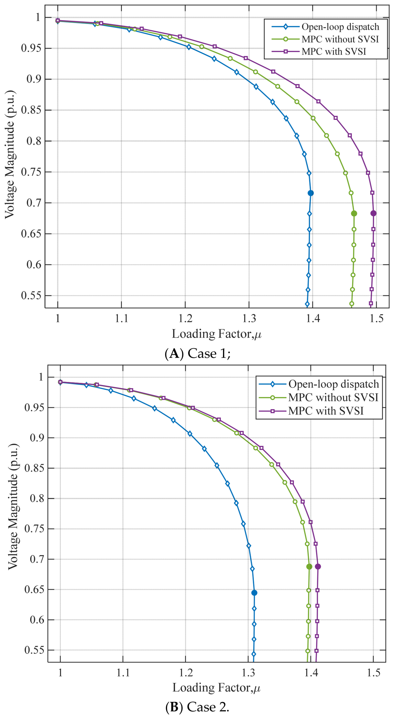
To independently verify the effectiveness of the proposed SVSI, continuation power flow (CPF) is further employed to evaluate the static voltage stability margin. For each case, the operating instant with the maximum SVSI under open-loop dispatch is selected as the representative operating point, and the same instant is used for the three scheduling methods to ensure a consistent comparison.
During the CPF calculation, the active and reactive loads on the distribution-network side are increased proportionally while maintaining their original power factors:
P L , i ( μ ) = μ P L , i 0 ,
Q L , i ( μ ) = μ Q L , i 0 ,
where P L , i 0 and Q L , i 0 are the initial active and reactive loads, respectively, and μ is the loading factor. The initial operating point corresponds to μ = 1 . The critical loading factor μ c r i t is determined from the nose point of the P–V curve, and the corresponding loadability margin is defined as
M l o a d = μ c r i t 1 .
Figure 18 shows the P–V curves obtained by CPF under the three scheduling methods. In both cases, the P–V nose point shifts to a higher loading factor when MPC is applied. The operating point obtained by MPC with SVSI exhibits the highest critical loading factor, indicating the largest static voltage stability margin.
As shown in Table 6, in Case 1, the critical loading factor increases from 1.420 under open-loop dispatch to 1.490 under MPC with SVSI, while the corresponding loadability margin increases from 0.420 to 0.490. In Case 2, the critical loading factor increases from 1.300 to 1.420, and the loadability margin increases from 0.300 to 0.420. The difference between the two MPC schemes in Case 2 is relatively small, which is consistent with their close SVSI values.
Overall, the CPF results show that lower SVSI values are consistently associated with larger critical loading factors and loadability margins. Therefore, the independent CPF results confirm that the reduction in SVSI corresponds to an improvement in system loadability and static voltage stability margin under the investigated operating conditions.

6. Conclusions

This paper addresses the challenges caused by the integration of high-penetration distributed generation into distribution networks, including bidirectional power-flow variations, accumulated forecasting errors, and reduced static voltage stability margins. A multi-time-scale rolling optimal control method for distribution networks considering static voltage stability is proposed. Based on model predictive control (MPC), a coordinated control framework combining long-time-scale baseline scheduling, short-time-scale rolling optimization, and real-time feedback correction is developed. Moreover, a static voltage stability index (SVSI) based on local network equivalencing is embedded into the rolling optimization process, enabling the coordinated consideration of economic operation, renewable energy accommodation, and static voltage stability constraints. The main conclusions are as follows.
(1)
The proposed multi-time-scale rolling optimal control method can effectively improve the limited adaptability of conventional open-loop scheduling to forecasting errors. Long-time-scale scheduling provides a baseline plan with global economic performance, while short-time-scale MPC performs rolling correction of control variables according to ultra-short-term forecasts and real-time measurements. As a result, the output adjustments of distributed generation, energy storage systems, and flexible loads become smoother. Under both slowly varying and rapidly fluctuating wind and photovoltaic generation scenarios, the proposed method reduces the impact of intermittent renewable energy fluctuations on scheduling results and improves the real-time adaptability of active distribution network operation and control.
(2)
The SVSI based on local network equivalencing can adapt to complex power-flow direction variations caused by high-penetration distributed generation. By equivalently processing multiple power-inflow and power-outflow branches around a node, the proposed SVSI calculation method overcomes the limitations of conventional single-branch indices under reverse power flow or multi-branch coupling conditions. Therefore, it provides effective support for the online assessment of static voltage stability boundaries in distribution networks.
(3)
Embedding the SVSI constraint into the MPC rolling optimization model can improve the static voltage stability margin while maintaining scheduling economy and renewable energy accommodation capability. The case study results show that, under the slowly varying wind and photovoltaic generation scenario, the maximum SVSI decreases from 0.05666 under conventional open-loop scheduling to 0.05465. Under the rapidly fluctuating renewable energy scenario, the maximum SVSI decreases from 0.06229 to 0.05860, and the average SVSI also decreases accordingly. These results indicate that the proposed method can effectively prevent the system operating point from approaching the static voltage stability boundary, with a more pronounced stability improvement under scenarios involving abrupt renewable energy variations.
In summary, by combining multi-time-scale rolling optimization with online static voltage stability constraints, the proposed method improves the adaptability of distribution networks to renewable energy fluctuations and load forecasting deviations, while enhancing the static voltage security level of the system. Future research will further consider three-phase unbalance characteristics, communication delays, operation constraints of discrete voltage regulation devices, and multi-area coordinated control, so as to improve the engineering applicability of the proposed method in practical active distribution network operation.


Author Contributions

Conceptualization, S.Y., F.Z. and T.N.; Methodology, S.Y., F.Z., J.J. and T.N.; Software, J.Z., Y.Z. and J.J.; Validation, J.Z., Y.Z. and S.D.; Formal Analysis, J.Z., Y.Z. and J.J.; Investigation, J.Z. and S.D.; Resources, F.Z., L.Y. and T.N.; Data Curation, J.Z. and Y.Z.; Writing—Original Draft Preparation, J.Z.; Writing—Review and Editing, J.Z., J.J., Y.Z. and T.N.; Visualization, J.Z. and Y.Z.; Supervision, T.N.; Project Administration, F.Z. and T.N.; Funding Acquisition, S.Y. All authors have read and agreed to the published version of the manuscript.

Funding

This research was funded by the science and technology project of State Grid Zhejiang Electric Power Co., Ltd. (Research on Intelligent Generation and Multi-Level Frequency and Voltage Coordinated Control Methods for Complex Multi-Scenario Operation Modes Including High Proportion of Centralized/Distributed New Energy Sources), grant number B311DS25Z017.

Data Availability Statement

The original contributions presented in this study are included in the article. Further inquiries can be directed to the corresponding author.

Conflicts of Interest

Authors Shize Ye and Feng Zhang were employed by State Grid Zhejiang Electric Power Co., Ltd. Research Institute. Author Lin Ye was employed by State Grid Zhejiang Electric Power Co., Ltd. Author Shitong Dai was employed by State Grid Xiangshan Power Supply Company. The remaining authors declare that the research was conducted in the absence of any commercial or financial relationships that could be construed as a potential conflict of interest. The State Grid Zhejiang Electric Power Co., Ltd. had no role in the design of the study; in the collection, analyses, or interpretation of data; in the writing of the manuscript, or in the decision to publish the results.

References

  1. Ackermann, T.; Andersson, G.; Söder, L. Distributed generation: A definition. Electr. Power Syst. Res. 2001, 57, 195–204. [Google Scholar] [CrossRef] [Scilit]
  2. Pepermans, G.; Driesen, J.; Haeseldonckx, D.; Belmans, R.; D’haeseleer, W. Distributed generation: Definition, benefits and issues. Energy Policy 2005, 33, 787–798. [Google Scholar] [CrossRef] [Scilit]
  3. El-Khattam, W.; Hegazy, Y.G.; Salama, M.M.A. An integrated distributed generation optimization model for distribution system planning. IEEE Trans. Power Syst. 2005, 20, 1158–1165. [Google Scholar] [CrossRef] [Scilit]
  4. Lopes, J.A.P.; Hatziargyriou, N.; Mutale, J.; Djapic, P.; Jenkins, N. Integrating distributed generation into electric power systems: A review of drivers, challenges and opportunities. Electr. Power Syst. Res. 2007, 77, 1189–1203. [Google Scholar] [CrossRef] [Scilit]
  5. Atwa, Y.M.; El-Saadany, E.F.; Salama, M.M.A.; Seethapathy, R. Optimal renewable resources mix for distribution system energy loss minimization. IEEE Trans. Power Syst. 2010, 25, 360–370. [Google Scholar] [CrossRef] [Scilit]
  6. Georgilakis, P.S.; Hatziargyriou, N.D. Optimal distributed generation placement in power distribution networks: Models, methods, and future research. IEEE Trans. Power Syst. 2013, 28, 3420–3428. [Google Scholar] [CrossRef] [Scilit]
  7. Camacho, E.F.; Bordons, C. Model Predictive Control, 2nd ed.; Springer: London, UK, 2007. [Google Scholar] [CrossRef] [Scilit]
  8. Venkat, A.N.; Hiskens, I.A.; Rawlings, J.B.; Wright, S.J. Distributed MPC strategies with application to power system automatic generation control. IEEE Trans. Control Syst. Technol. 2008, 16, 1192–1206. [Google Scholar] [CrossRef] [Scilit]
  9. Xie, L.; Ilić, M.D. Model predictive dispatch in electric energy systems with intermittent resources. In Proceedings of the 2008 IEEE International Conference on Systems, Man and Cybernetics, Singapore, 12–15 October 2008; pp. 42–47. [Google Scholar] [CrossRef] [Scilit]
  10. Xie, L.; Ilić, M.D. Model predictive economic/environmental dispatch of power systems with intermittent resources. In Proceedings of the 2009 IEEE Power & Energy Society General Meeting, Calgary, AB, Canada, 26–30 July 2009; pp. 1–6. [Google Scholar] [CrossRef] [Scilit]
  11. Xia, X.; Zhang, J.; Elaiw, A.M. A model predictive control approach to dynamic economic dispatch problem. In Proceedings of the 2009 IEEE Bucharest PowerTech, Bucharest, Romania, 28 June–2 July 2009; pp. 1–7. [Google Scholar] [CrossRef] [Scilit]
  12. Elaiw, A.M.; Xia, X.; Shehata, A.M. Application of model predictive control to optimal dynamic dispatch of generation with emission limitations. Electr. Power Syst. Res. 2012, 84, 31–44. [Google Scholar] [CrossRef] [Scilit]
  13. Morstyn, T.; Hredzak, B.; Aguilera, R.P.; Agelidis, V.G. Model predictive control for distributed microgrid battery energy storage systems. IEEE Trans. Control Syst. Technol. 2018, 26, 1107–1114. [Google Scholar] [CrossRef] [Scilit]
  14. Garcia-Torres, F.; Zafra-Cabeza, A.; Silva, C.; Grieu, S.; Darure, T.; Estanqueiro, A. Model predictive control for microgrid functionalities: Review and future challenges. Energies 2021, 14, 1296. [Google Scholar] [CrossRef] [Scilit]
  15. Su, W.; Wang, J.; Zhang, K.; Huang, A.Q. Model predictive control-based power dispatch for distribution system considering plug-in electric vehicle uncertainty. Electr. Power Syst. Res. 2014, 106, 29–35. [Google Scholar] [CrossRef] [Scilit]
  16. Parisio, A.; Rikos, E.; Glielmo, L. A model predictive control approach to microgrid operation optimization. IEEE Trans. Control Syst. Technol. 2014, 22, 1813–1827. [Google Scholar] [CrossRef] [Scilit]
  17. Raimondi Cominesi, S.; Farina, M.; Giulioni, L.; Picasso, B.; Scattolini, R. A two-layer stochastic model predictive control scheme for microgrids. IEEE Trans. Control Syst. Technol. 2018, 26, 1–13. [Google Scholar] [CrossRef] [Scilit]
  18. Ghiasi, M.; Niknam, T.; Dehghani, M.; Baghaee, H.R.; Wang, Z.; Ghanbarian, M.M.; Blaabjerg, F.; Dragicevic, T. Multipurpose FCS model predictive control of VSC-based microgrids for islanded and grid-connected operation modes. IEEE Syst. J. 2023, 17, 2558–2569. [Google Scholar] [CrossRef] [Scilit]
  19. Yang, L.; Sun, X.; Cao, X.; Chen, M.; Guan, X. Joint chance-constrained coordinated scheduling for electricity–heat coupled systems considering hydrogen storage. Energy Internet 2024, 1, 99–111. [Google Scholar] [CrossRef] [Scilit]
  20. Kessel, P.; Glavitsch, H. Estimating the voltage stability of a power system. IEEE Trans. Power Deliv. 1986, 1, 346–354. [Google Scholar] [CrossRef] [Scilit]
  21. Ajjarapu, V.; Christy, C. The continuation power flow: A tool for steady state voltage stability analysis. IEEE Trans. Power Syst. 1992, 7, 416–423. [Google Scholar] [CrossRef] [Scilit]
  22. Gao, B.; Morison, G.K.; Kundur, P. Voltage stability evaluation using modal analysis. IEEE Trans. Power Syst. 1992, 7, 1529–1542. [Google Scholar] [CrossRef] [Scilit] [PubMed]
  23. Van Cutsem, T. Voltage instability: Phenomena, countermeasures, and analysis methods. Proc. IEEE 2000, 88, 208–227. [Google Scholar] [CrossRef] [Scilit]
  24. Chakravorty, M.; Das, D. Voltage stability analysis of radial distribution networks. Int. J. Electr. Power Energy Syst. 2001, 23, 129–135. [Google Scholar] [CrossRef] [Scilit]
  25. Musirin, I.; Abdul Rahman, T.K. Novel fast voltage stability index for voltage stability analysis in power transmission system. In Proceedings of the 2002 Student Conference on Research and Development: Globalizing Research and Development in Electrical and Electronics Engineering, Shah Alam, Malaysia, 16–17 July 2002; pp. 265–268. [Google Scholar] [CrossRef] [Scilit]
  26. Song, Y.; Hill, D.J.; Liu, T. Static voltage stability analysis of distribution systems based on network-load admittance ratio. IEEE Trans. Power Syst. 2019, 34, 2270–2280. [Google Scholar] [CrossRef] [Scilit]
  27. Wang, Z.; Cui, B.; Wang, J. A necessary condition for power flow insolvability in power distribution systems with distributed generators. IEEE Trans. Power Syst. 2017, 32, 1440–1450. [Google Scholar] [CrossRef] [Scilit]
  28. Aolaritei, L.; Bolognani, S.; Dörfler, F. Hierarchical and distributed monitoring of voltage stability in distribution networks. IEEE Trans. Power Syst. 2018, 33, 6705–6714. [Google Scholar] [CrossRef] [Scilit]
  29. Mudaliyar, S.; Mishra, S. Real-time coordinated control of low-voltage DC distribution network with soft opening point. IEEE Trans. Power Electron. 2021, 36, 7123–7137. [Google Scholar] [CrossRef] [Scilit]
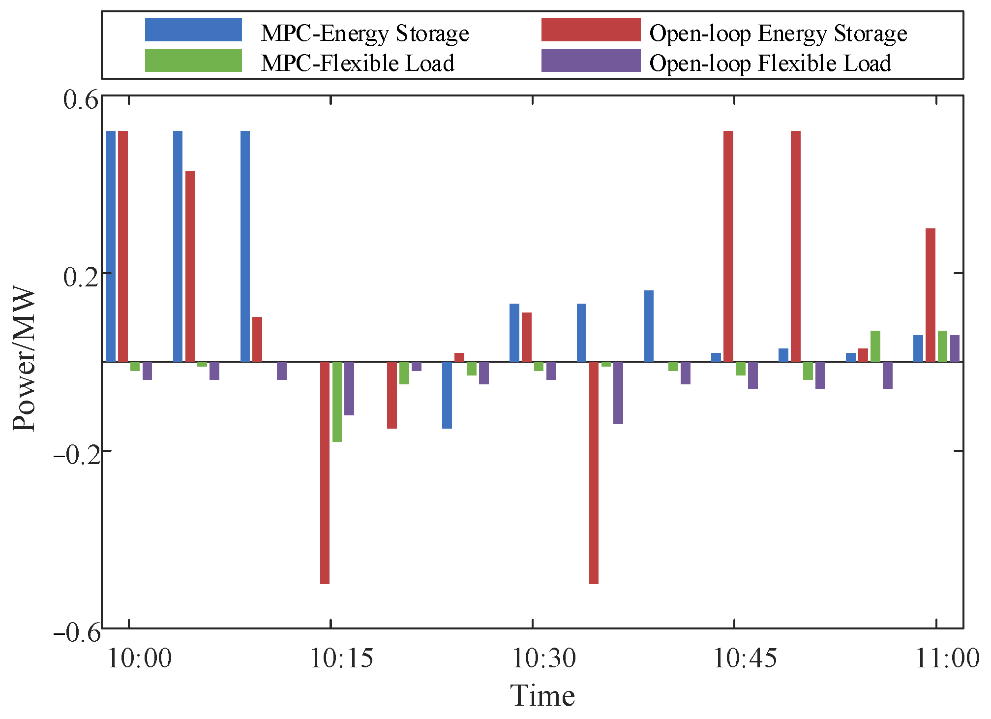
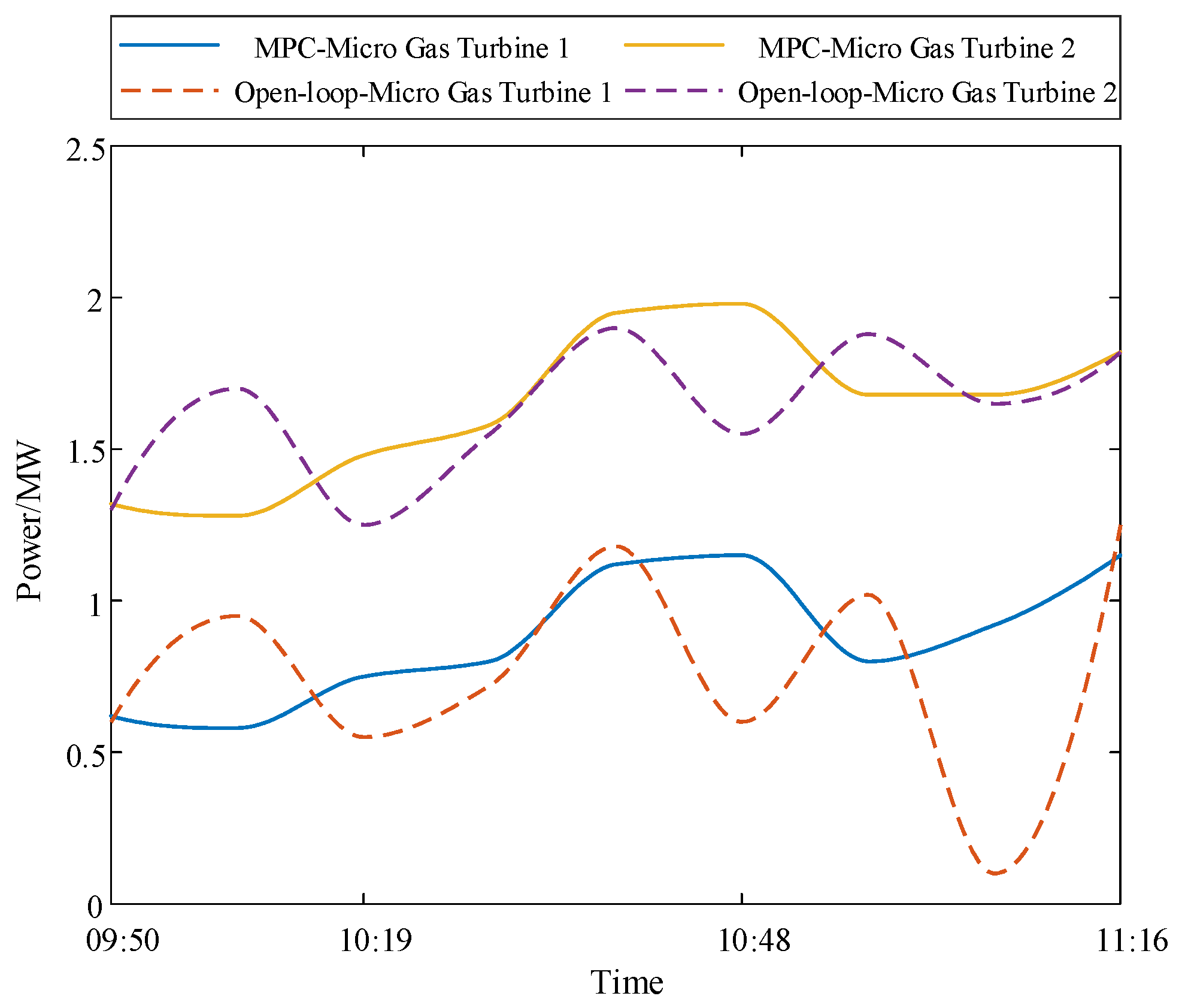
  30. Liu, C.; Li, Z. Offer-making model for aggregators of prosumers under network security constraints and complex market environment. Energy Internet 2025, 2, 313–327. [Google Scholar] [CrossRef] [Scilit]
  31. Jalali, A.; Aldeen, M. Risk-based stochastic allocation of ESS to ensure voltage stability margin for distribution systems. IEEE Trans. Power Syst. 2019, 34, 1264–1277. [Google Scholar] [CrossRef] [Scilit]
  32. Eajal, A.A.; Yazdavar, A.H.; El-Saadany, E.F.; Ponnambalam, K. On the loadability and voltage stability of islanded AC–DC hybrid microgrids during contingencies. IEEE Syst. J. 2019, 13, 4248–4259. [Google Scholar] [CrossRef] [Scilit]
  33. Wang, C.; Cui, B.; Wang, Z.; Gu, C. SDP-based optimal power flow with steady-state voltage stability constraints. IEEE Trans. Smart Grid 2019, 10, 4637–4647. [Google Scholar] [CrossRef] [Scilit]
  34. Bakhtvar, M.; Keane, A. Allocation of wind capacity subject to long-term voltage stability constraints. IEEE Trans. Power Syst. 2016, 31, 2404–2414. [Google Scholar] [CrossRef] [Scilit]
  35. Sun, Q.; Hu, J.; Wang, R.; Zhang, H. Source–load cooperative frequency regulation based on virtual synchronous/asynchronous machine concept. Energy Internet 2024, 1, 188–199. [Google Scholar] [CrossRef] [Scilit]
  36. Yang, Y.; Dong, W.; Ye, S.; Ji, J.; Zheng, J.; Zeng, Y.; Niu, T. A Transmission–Distribution Coordinated Optimal Scheduling Strategy Considering Short-Term Voltage Stability and Supply–Demand Flexibility Balance. Processes 2026, 14, 889. [Google Scholar] [CrossRef] [Scilit]
  37. Yang, Y.; Wu, W. A Distributionally Robust Optimization Model for Real-Time Power Dispatch in Distribution Networks. IEEE Trans. Smart Grid 2019, 10, 3743–3752. [Google Scholar] [CrossRef] [Scilit]
  38. Zhang, Y.; Ai, X.; Fang, J.; Wen, J.; He, H. Data-Adaptive Robust Optimization Method for the Economic Dispatch of Active Distribution Networks. IEEE Trans. Smart Grid 2019, 10, 3791–3800. [Google Scholar] [CrossRef] [Scilit]
Figure 1. Multi-time-scale MPC-based scheduling architecture with SVSI constraints. Arrows indicate the flow of scheduling information, control actions, and measurement feedback among the three layers.
Processes 14 02877 g001
Figure 2. Line model.
Processes 14 02877 g002
Figure 3. Local network model.
Processes 14 02877 g003
Figure 4. Equivalent local network model.
Processes 14 02877 g004
Figure 5. Online SVSI calculation process based on local network equivalencing.
Processes 14 02877 g005
Figure 6. Flowchart of the rolling correction process for the static voltage stability boundary.
Processes 14 02877 g006
Figure 7. Combination of a transmission system (IEEE 14 bus system) with two (modified IEEE 13 node feeders) distribution systems [36].
Processes 14 02877 g007
Figure 8. Load, wind power, and photovoltaic power profiles under the slow-variation scenario.
Processes 14 02877 g008
Figure 9. Long-Time-Scale Scheduled Active Power Outputs of Distributed Generators.
Processes 14 02877 g009
Figure 10. Short-Time-Scale Active Power Outputs of Distributed Generators.
Processes 14 02877 g010
Figure 11. Micro Gas Turbine Active Power Output in Case Study 1.
Processes 14 02877 g011
Figure 12. Energy Storage and Flexible Load Optimization Results in Case Study 1.
Processes 14 02877 g012
Figure 13. Load, wind power, and photovoltaic power profiles under the fast-fluctuation scenario.
Processes 14 02877 g013
Figure 14. Micro Gas Turbine Active Power Output in Case Study 2.
Processes 14 02877 g014
Figure 15. Tie-Line Power Exchange with the Main Grid in Case Study 2.
Processes 14 02877 g015
Figure 16. Energy Storage and Flexible Load Optimization Results in Case Study 2.
Processes 14 02877 g016
Figure 17. Variation curves of the system maximum SVSI under different scheduling methods.
Processes 14 02877 g017
Figure 18. P–V curves obtained by continuation power flow under different scheduling methods.
Processes 14 02877 g018
Table 1. Parameters of Microturbines and Flexible Loads.
ParameterPhysical MeaningUnitValue
α i Flexible-load cost coefficientp.u.2/$5
β i Flexible-load characteristic coefficientp.u.0.31
λ ess Energy-storage scheduling cost coefficient$/p.u.20.27/0.32/0.42
a1Quadratic cost coefficient of DG1$/p.u.20.29
b1Linear cost coefficient of DG1$/p.u.0.05
c1Constant cost coefficient of DG1$0.78
a2Quadratic cost coefficient of DG2$/p.u.20.30
b2Linear cost coefficient of DG2$/p.u.0.03
c2Constant cost coefficient of DG2$0.75
Table 2. Performance of the Proposed Method under Different Representative Operating Periods.
ScenarioTime PeriodOperating CharacteristicMaximum SVSIMinimum Bus Voltage/p.u.Energy Loss/MWhRenewable Energy Curtailment/MWhOperating Cost/$
Morning ramping06:00–08:00Load and PV ramping up0.056920.993100.19760.010129.4
Daytime slow variation10:00–12:00High PV, slow RES variation0.054650.993820.20280.015125.3
Daytime rapid fluctuation10:00–12:00Rapid wind/PV variation0.058600.991680.19130.019128.7
Evening peak18:00–20:00PV decline and load increase0.061740.990620.21470.003136.5
Table 3. Operating Results under Different Renewable Energy Penetration Levels.
Renewable Energy Penetration LevelWind Power Capacity/kWPV Capacity/kWMaximum SVSIMinimum Bus Voltage/p.u.Energy Loss/MWhRenewable Energy Curtailment/MWhOperating Cost/$
80%8004000.1460.9620.1860.000131.6
100% (Base Case)10005000.1530.9580.1740.008125.3
120%12006000.1650.9530.1690.026121.8
140%14007000.1810.9470.1770.058120.9
Table 4. Performance Comparison under Different MPC Parameter Settings.
CaseControl Interval/minPrediction Horizon/minM = NWeight SettingMaximum SVSIMinimum Voltage/p.u.Operating Cost/$Renewable Energy Utilization/%Computation Time/s
15102Q00.1610.954127.198.20.58
25153Q00.1530.958125.398.90.84
35204Q00.1510.959124.999.01.19
410202Q00.1690.951127.898.00.66
515302Q00.1780.946130.497.20.71
65153Q00.1580.955124.799.00.82
75153Q00.1490.961126.698.70.87
Table 5. Comparison of static voltage stability indices under different scheduling methods.
CaseMethod S V S I m a x S V S I ¯ U m i n / p . u . E l o s s / k W h E c u r / M W h
Case 1Open-loop dispatch0.056660.051150.99376204.0180.000
Case 1MPC without SVSI0.055670.051040.99382204.6880.000
Case 1MPC with SVSI0.054650.050830.99382202.8100.015
Case 2Open-loop dispatch0.062290.050250.99159204.4790.000
Case 2MPC without SVSI0.058700.048820.99168191.1650.000
Case 2MPC with SVSI0.058600.048770.99168191.2570.019
Table 6. Independent validation of SVSI using continuation power flow.
CaseScheduling MethodSVSI at t Critical Loading Factor μ c r i t Loadability Margin M l o a d
Case 1Open-loop dispatch0.056661.4200.420
Case 1MPC without SVSI0.055021.4500.450
Case 1MPC with SVSI0.054621.4900.490
Case 2Open-loop dispatch0.062291.3000.300
Case 2MPC without SVSI0.058561.4100.410
Case 2MPC with SVSI0.058471.4200.420
Disclaimer/Publisher’s Note: The statements, opinions and data contained in all publications are solely those of the individual author(s) and contributor(s) and not of MDPI and/or the editor(s). MDPI and/or the editor(s) disclaim responsibility for any injury to people or property resulting from any ideas, methods, instructions or products referred to in the content.