Fast Generation of Feasible Unit Commitment Schedules Based on Standardized Net-Load Trajectory Similarity and Historical Schedule Transfer

Abstract

High penetration of wind and photovoltaic generation reshapes power system net-load profiles and increases the computational burden of repeatedly solving security-constrained unit commitment problems under multiple renewable scenarios. This paper proposes a fast schedule generation method based on historical schedule transfer. A library is constructed by pairing feasible unit commitment schedules with their corresponding 24 h net-load trajectories. For a target day, hour-wise, standardized net-load trajectories are compared using Euclidean distance, and the Top-K most similar historical schedules are selected as candidates. Each candidate is verified under the target-day operating conditions. When no candidate satisfies the feasibility or economic requirements, a limited-perturbation model is applied to repair the retrieved schedule with minimal changes in unit statuses. Case studies show that the proposed method effectively transfers historical commitment patterns, maintains operational feasibility and near-optimal economic performance, and reduces the computational effort required for unit commitment schedule generation.

1. Introduction

With the accelerated transition of power systems toward low-carbon and sustainable operation, renewable energy sources such as wind and solar power have accounted for an increasing share of the generation mix. Renewable generation is characterized by strong variability, intermittency, and anti-peak characteristics. Its large-scale integration not only reshapes the power supply–demand balance but also intensifies the operating pressure on conventional units in terms of peak-shaving and valley-filling, fast ramping, reserve provision, and network security. In studies addressing the duck curve challenge, reference [1] pointed out that the intra-day concentration of photovoltaic (PV) generation depresses daytime net load and produces a strong ramping requirement in the evening, which means that the temporal distribution of renewable generation directly changes the regulation demand faced by conventional units.

From the perspective of day-ahead unit commitment (UC) and security-constrained unit commitment (SCUC), renewable energy integration primarily affects power system operation by reshaping the net-load curve. As a result, system dispatch is gradually shifting from conventional load-following operation to net-load-driven operation. The increasing variability and peak-valley difference in the net-load curve caused by renewable energy integration impose greater regulation requirements on conventional units and generally increase the difficulty of solving the UC problem. In this context, rapidly identifying SCUC results that can accommodate renewable energy output and load variations has become a key challenge for improving day-ahead dispatch efficiency and supporting multi-scenario operational analysis.

The UC models of power systems generally lead to a large-scale mixed integer linear programming (MILP) problem, where unit ON/OFF decisions, ramping limits, reserve provision, and network power-flow constraints are considered simultaneously. Reference [2] provided a systematic review of the modeling approaches and solution challenges of SCUC problems. It pointed out that commitment variables, network constraints, and uncertainty treatment are core difficulties in day-ahead SCUC models. On this basis, reference [3] further compared different UC formulations and showed that the representation of start-up and shut-down logic, ramping constraints, and minimum ON/OFF time constraints directly affects solution efficiency and feasible-solution quality.

Because renewable energy integration makes day-ahead UC highly dependent on uncertain wind power, PV generation, and load conditions, multi-scenario analysis has become an important tool for evaluating system operation under different net-load patterns. Against this background, scenario generation has been widely used to characterize renewable uncertainty in power system dispatch [4,5,6,7,8,9]. Reference [10] systematically reviewed methods of quantitatively evaluating generated scenarios and emphasized that scenario quality should be evaluated in relation to downstream power system operation. In fact, generated scenarios are generally used as external inputs to UC models, and the corresponding unit commitment schedules can only be obtained after solving the optimization problem. However, repeatedly solving UC models over numerous scenarios inevitably brings a heavy computational burden. In practice, different scenarios often produce the same or only marginally different unit commitment schedules, namely ON/OFF statuses, resulting in only minor changes in the objective value. With the development of deep learning, increasing attention has been paid to directly generating or predicting UC solutions based on scenario inputs. By learning the mapping relationship between operating scenarios and historical optimization solutions, machine-learning-based solving methods can provide candidate unit commitment schedules without repeatedly solving the full UC problem, thereby reducing unnecessary solving efforts and supporting fast multi-scenario operational analysis. Moreover, in applications that require repeatedly solving partially modified UC problems, such as market-oriented gaming models, machine-learning-based solving methods can serve as surrogates that rapidly return candidate solutions during the iterative solution process.

Machine-learning-assisted methods attempt to extract reusable solutions from historical optimization instances and transfer them to new UC cases. Earlier studies mainly embedded machine-learning models into the optimization process. Typical applications include identifying critical commitment variables, screening inactive units, predicting active constraints, and providing warm-start solutions. Reference [11] integrated machine learning within a decomposition-and-coordination optimization framework to learn solutions to UC subproblems for speeding up the convergence of the iterative process. Reference [12] learned stable commitment variables from branch-and-bound information and fixed a subset of the binary variables before optimization. Beyond fixing binary variables, the network constraints can also be pruned. Reference [13] proposed a cost-driven screening method to identify inactive or redundant transmission constraints in the UC problem. In addition to reducing the problem size, reference [14] extracted information from historical SCUC instances to predict redundant constraints and good initial feasible solutions, thereby reducing the problem size and providing warm starts for MIP solvers. In addition, some machine-learning-based strategies, in a more general setting, are used to guide the branching process of MILP problems by exploiting the special structure of UC formulations. Reference [15] trained a graph convolutional network to imitate strong branching variable selection policies and reference [16] learned branching rules for MILP problems. The two methods can accelerate the tree search without modifying the model.

More recent studies have further attempted to directly learn the mapping from operating conditions, such as load profiles, renewable generation scenarios, and net-load profiles, to UC solutions, so that candidate unit commitment schedules can be obtained without solving the full UC model. For example, reference [17] established a predictive-prescription framework in which a boosting ensemble maps contextual operating features to commitment decisions, so that a schedule is prescribed directly from historical data rather than re-optimized for each new condition. Reference [18] developed a graph neural network data-augmentation framework, where the graph neural network is used to capture the structural relationships among system components and enrich the learning process for predicting near-optimal UC schedules. In fact, the solutions directly produced by learning models are likely to violate operational constraints, and therefore usually need to be combined with feasibility recovery or solution correction models. Therefore, feasibility layers, post-processing procedures, and optimization-based correction mechanisms are often required to recover feasible schedules [19,20]. The fast generation of feasible solutions to UC models under diverse renewable scenarios remains challenging, let alone a guarantee of optimality. Moreover, the commitment schedules generated may deviate significantly from practical operating patterns, making them less consistent with operators’ experience and actual dispatch practices. In fact, system operators often prefer commitment patterns that remain close to previously implemented and validated schedules. Such historical schedules may implicitly incorporate operator experience and system-specific security considerations that are difficult to represent fully in a standard UC model, including short-circuit strength, transient stability, voltage stability, and other practical operating requirements.

Machine-learning-assisted methods can accelerate the UC solving process, but they generally still require the UC problem to be re-optimized with partially fixed commitment variables, relaxed inactive constraints, or warm-start settings. By contrast, direct solution generation methods avoid repeated solving, but the generated commitment schedules are not necessarily feasible and may violate unit operational constraints, particularly minimum ON/OFF time limits. In this case, the unit commitment schedules are required to be adjusted. One alternative is to reuse the unit commitment schedules of historical days. Since these schedules are produced by a full UC model, they already satisfy the relevant operational constraints and reflect actual dispatch practices. The key issue is therefore how to identify a suitable historical day for reuse. Under high renewable energy penetration, the net-load curve provides an effective basis for the selection. Net load is defined as the system load minus the available renewable power output, and represents the residual demand to be supplied by conventional units. Since this residual demand determines the required generation level, ramping capability, and reserve provision, it strongly affects unit commitment decisions. Therefore, historical days with similar net-load curves are likely to have similar peaks, valleys, and ramping patterns, leading to similar commitment schedules.

Based on this idea, this paper first constructs a library of commitment schedules from historical UC cases. For each historical day, the net-load trajectory is calculated from the load demand and available renewable power. Each record in the library contains the commitment schedule, while being labeled by a 24 h net-load trajectory. On this basis, day-to-day similarity is measured using the Euclidean distance between standardized 24 h net-load trajectories, so that the comparison reflects both the relative hourly level and the intra-day shape of the net-load trajectories. For a target day, the K historical days with the most similar standardized net-load trajectories, referred to as the Top-K similar days, are retrieved, and their commitment schedules are used as candidate solutions. Each candidate is verified by fixing the unit ON/OFF statuses and re-optimizing dispatch. Infeasible or high-cost candidates are repaired through a limited-perturbation repair model. The resulting schedules preserve the main structure of historical UC solutions, while satisfying operational constraints and achieving costs close to the full UC benchmark.

Unlike existing machine-learning-assisted methods that partly support variable fixing, constraint screening, or warm starts, the proposed method directly transfers complete historical schedules to the target day. Since these schedules are obtained from previously solved UC or SCUC problems, they preserve feasible intertemporal operating patterns. The novelty lies in a retrieval, verification, and repair framework that selects historical schedules based on standardized net-load similarity, verifies them under target day conditions, and applies limited repair only when necessary.

The main contributions of this paper are summarized as follows:

• A training-free schedule transfer method is proposed to retrieve complete, solver-validated historical UC schedules based on standardized net-load trajectory similarity, avoiding the prediction of individual binary variables.
• A strategy combining candidate retrieval, feasibility verification, and limited repair is developed. The Top-K candidates are evaluated through fixed binary dispatch and adjusted only when necessary, ensuring feasibility while maintaining economic performance and computational efficiency.

The remainder of this paper is organized as follows. Section 2 establishes the day-ahead unit commitment and security-constrained unit commitment models. Section 3 presents the proposed commitment schedule generation method based on the day-to-day similarity measured by the Euclidean distance of net-load trajectories and the limited-perturbation repair model. Section 4 evaluates the method on a modified IEEE 118-bus system in terms of strict feasibility, similarity of unit ON/OFF statuses, economic deviation, and computational efficiency. Section 5 concludes the paper.

2. The Unit Commitment and Security-Constrained Unit Commitment Models

To obtain commitment schedules of conventional units under different net-load profiles, this section first introduces the day-ahead UC model and further extends it with security constraints to build the SCUC model. The two models consider a 24 h scheduling horizon with hourly time resolution. The UC and SCUC models account for operating limits on the unit level and the system level. For the former, the constraints include conventional unit ON/OFF statuses, start-up and shut-down logic, minimum ON/OFF time, power output ranges, and unit ramping capabilities. For the latter, the constraints include system balance, system reserve requirements, and transmission line flow limits.

The UC model minimizes the system operating cost while considering the renewable power curtailment, as shown in (1). The system operating cost $c^{OP}$ and the renewable power curtailment penalty cost $c^{PN}$ are respectively given in Equations (2) and (3).

$$\mathit{min}(c^{OP}+c^{PN})$$

(1)

$$c^{OP}={{\displaystyle \sum }}_{n=1}^N{{\displaystyle \sum }}_{t=1}^T\left[{{\displaystyle \sum }}_{k=1}^{K_n}{b}_{n,k}·p_{n,k,t}+C_n^{FX}·u_{n,t}+C_n^{ST}·y_{n,t}+C_n^{SD}·z_{n,t}\right]$$

(2)

$$c^{PN}=K^{RE}·p^{C,RE}$$

(3)

$$p^{C,RE}={{\displaystyle \sum }}_{v=1}^V{{\displaystyle \sum }}_{t=1}^T\left(P_{v,t}^{RE}-p_{v,t}^{RE}\right)$$

(4)

In (2), $N$ denotes the number of thermal units, and $T$ denotes the number of hours in the scheduling time horizon; $b_{n,k}$ is the cost coefficient of the segment $k$ of conventional unit $n$; $C_n^{FX}$, $C_n^{ST}$, and $C_n^{SD}$ represent the fixed operating cost, start-up cost, and shut-down cost of conventional unit $n$, respectively; and $u_{n,t}$ denotes the ON/OFF statuses of conventional unit $n$ at hour $t$. When $u_{n,t}=1$, the unit is ON; otherwise, it is OFF. $y_{n,t}$ and $z_{n,t}$ are respectively binary indicators representing the start-up and shut-down of thermal unit $n$ at hour $t$. In (3), variable $p^{C,RE}$, as calculated in (4), denotes the total curtailed renewable energy, and $K^{\mathrm{RE}}$ denotes the corresponding penalty-cost coefficients for renewable power curtailment. In (4), $p_{v,t}^{RE}$ denotes the available renewable power at hour $t$; and $p_{v,t}^{\mathrm{RE}}$ denotes the dispatched renewable power at hour $t$. We use $V$ to denote the number of renewable sources, including wind farms and PV stations.

The constraints are formulated as shown in (5)–(24).

• Dispatchable range constraints for renewable energy

Constraint (5) requires the dispatchable renewable power at hour $t$ of renewable source $v$ to be no greater than the available renewable power in that period.

$$0\le p_{v,t}^{\mathrm{RE}}\le P_{v,t}^{\mathrm{RE}}$$

(5)

• Operational constraints of conventional units

The constraints for conventional unit power output are formulated as in (6)–(8), where $p_{n,k,t}$ denotes the output of conventional unit $n$ in segment $k$ at hour $t$; $G_n^{SEG}$ denotes the range of the segments for conventional unit $n$; and $K_n$ denotes the number of segments. Constraint (8) restricts the output of conventional unit $n$ at hour $t$, where $P_n^{LB}$ and $P_n^{UB}$ respectively denote the lower and upper bounds of the power output.

$$0\le p_{n,k,t}\le G_n^{SEG}·u_{n,t}$$

(6)

$$p_{n,t}={{\displaystyle \sum }}_{k=1}^{K_n}{p}_{n,k,t}+P_n^{LB}·u_{n,t}$$

(7)

$$P_n^{LB}·u_{n,t}\le p_{n,t}\le P_n^{UB}·u_{n,t}$$

(8)

The unit ramping constraints are given in (9) and (10), where $R^{+}$ and $R^{-}$ respectively denote the upward and downward ramping rates of conventional unit $n$, and ${\Delta }_{30}$ denotes the 30 min ramping interval within each hourly time interval.

$$p_{n,t-1}-p_{n,t}\le R_n^{-}·{\Delta }_{30}·u_{n,t}+P_n^{LB}·z_{n,t}$$

(9)

$$p_{n,t}-p_{n,t-1}\le R_n^{+}·{\Delta }_{30}·u_{n,t-1}+P_n^{LB}·y_{n,t}$$

(10)

The start-up and shut-down constraints of unit $n$ are given in (11)–(13) with the typical “3-bin” formulation.

$$u_{n,1}=y_{n,1}-z_{n,1}$$

(11)

$$u_{n,t}-u_{n,t-1}=y_{n,t}-z_{n,t}$$

(12)

$$y_{n,t}+z_{n,t}\le 1$$

(13)

The minimum ON/OFF time constraints of conventional unit $n$ are given in (14) and (15). In constraints (14) and (15), $T{U}_n$ and $T{D}_n$ denote the minimum ON and OFF times of conventional unit $n$, respectively.

$${{\displaystyle \sum }}_{\tau =\mathit{max}(t-T{U}_n+1,1)}^t{y}_{n,\tau }\le u_{n,t}$$

(14)

$${{\displaystyle \sum }}_{\tau =\mathit{max}(t-T{D}_n+1,1)}^t{z}_{n,\tau }\le 1-u_{n,t}$$

(15)

The spinning reserve and operating reserve constraints are formulated as shown in (16) and (17). Spinning reserve is available only when a conventional unit is ON, whereas operating reserve is available when a unit is OFF. In (16) and (17), $r_{n,t}^{SR}$ and $r_{n,t}^{OR}$ denote the spinning reserve capacity and operating reserve capacity of conventional unit $n$ at hour $t$, respectively; ${\Delta }_5$ and ${\Delta }_{15}$ denote the 5 min and 15 min ramping intervals within each hourly time interval.

$$\left\{\begin{array}{c}{r}_{n,t}^{SR}\le \mathit{min}\left\{R_n^{+}·{\Delta }_5,P_{n,t}^{UB}-p_{n,t}\right\}\\ 0\le r_{n,t}^{SR}\le P_{n,t}^{UB}·u_{n,t}\end{array}\right.$$

(16)

$$\left\{\begin{array}{c}{r}_{n,t}^{OR}\le R_n^{+}·{\Delta }_{15}+P_n^{LB}\\ 0\le r_{n,t}^{OR}\le \left(1-u_{n,t}\right)·P_n^{UB}\end{array}\right.$$

(17)

• System power balance constraints

The system power balance is ensured by constraint (18), where $D_{d,t}$ denotes the demand of load $d$ at hour $t$.

$${{\displaystyle \sum }}_{n=1}^N{p}_{n,t}+{{\displaystyle \sum }}_{v=1}^V{p}_{v,t}^{RE}={{\displaystyle \sum }}_{d=1}^D{D}_{d,t}$$

(18)

• Transmission line flow constraints

The transmission line flow constraints are formulated as shown in (19) and (20), where $L_l^{UB}$ is the transmission capacity limit of line $l$; $f_{l,t}^0$ is the power flow of line $l$ under the normal operating state; and $S{F}_{l,n}^0$, $S{F}_{l,v}^0$, and $S{F}_{l,d}^0$ are the shift factors of conventional units, renewable sources, and loads under the normal operating state, respectively.

$$f_{l,t}^0={{\displaystyle \sum }}_{n=1}^{N}S{F}_{l,n}^0\hspace{0.17em}{p}_{n,t}+{{\displaystyle \sum }}_{v=1}^{V}S{F}_{l,v}^0\hspace{0.17em}{p}_{v,t}^{RE}\hspace{0.17em}-{{\displaystyle \sum }}_{d=1}^{D}S{F}_{l,d}^0\hspace{0.17em}{D}_{d,t}$$

(19)

$$-L_l^{UB}\le f_{l,t}^0\le L_l^{UB},\forall l,t$$

(20)

• System reserve requirement constraints

The system reserve requirement constraints are formulated as shown in (21) and (22), where $r_t^{SR}$ and $r_t^{OR}$ denote the spinning reserve and operating reserve requirements, respectively, at hour $t$.

$${{\displaystyle \sum }}_{n=1}^N{r}_{n,t}^{SR}\ge r_t^{SR}$$

(21)

$${{\displaystyle \sum }}_{n=1}^N{r}_{n,t}^{OR}\ge r_t^{OR}$$

(22)

The SCUC model is formulated by extending the UC model with transmission network security constraints to ensure secure system operation under contingencies. After incorporating the post-contingency network security constraint, a UC problem, (1)–(22), is transformed into an SCUC problem, namely (1)–(24).

• Post-contingency network security constraint

Constraints (23) and (24) are post-contingency network security constraints. In constraint (23), $f_{l,t}^c$ is the power flow of line $l$ under contingency $c$. $S{F}_{l,n}^c$, $S{F}_{l,v}^c$, and $S{F}_{l,d}^c$ are correspondingly the shift factors of conventional units, renewable sources, and loads under contingency $c$, respectively.

$$f_{l,t}^c={{\displaystyle \sum }}_{n=1}^{N}S{F}_{l,n}^c\hspace{0.17em}{p}_{n,t}+{{\displaystyle \sum }}_{v=1}^{V}S{F}_{l,v}^c\hspace{0.17em}{p}_{v,t}^{\mathrm{RE}}-{{\displaystyle \sum }}_{d=1}^{D}S{F}_{l,d}^c\hspace{0.17em}{D}_{d,t}$$

(23)

$$-L_l^{UB}\le f_{l,t}^c\le L_l^{UB},\forall l,t,c$$

(24)

3. Net-Load Euclidean Similarity-Based Commitment Schedule Generation

This section proposes a commitment schedule generation method. Net load, defined as system load minus available renewable generation, directly reflects the residual demand that is supplied by conventional units. Therefore, days with similar net-load trajectories usually have similar peak-valley patterns, ramping requirements, reserve requirements, and unit commitment structures. This provides the basis for reusing historical commitment schedules for a target day.

Based on this idea, we first construct a historical commitment schedule library from historical UC cases, where each historical net-load trajectory is paired with its feasible commitment schedule. Before retrieval, identical or near-identical commitment schedules are merged in the historical library to remove redundant candidates. For the target day, the Top-K most similar historical days are retrieved according to the standardized net-load trajectory, and their commitment schedules are used as candidates. The candidates are then evaluated by a verification model with fixed binary variables, and infeasible or high-cost candidates are further adjusted through a limited-perturbation repair model. Therefore, given the load demand and available renewable power sequences of the target day, the proposed method outputs a feasible hourly unit ON/OFF schedule by reusing and adapting historical unit commitment patterns rather than generating binary commitment variables from scratch.

3.1. Construction of the Historical Commitment Schedule Library

We use $\mathit{A}$ to denote the set of historical days and use $a$ to index them. For each historical day $a$, the load demand $D_{d,a,t}$ and available renewable power $P_{v,a,t}^{RE}$ are input into the full UC model to obtain the optimal unit ON/OFF statuses, start-up and shut-down statuses, and operating cost of the historical day.

The historical commitment schedule library can be expressed as follows:

$$H=\left\{\left({\mathit{L}}_a^N,{\mathit{u}}_a^{\ast },{\mathit{y}}_a^{\ast },{\mathit{z}}_a^{\ast },{\mathit{J}}_a^{\ast }\right)\mid a\in \mathit{A}\right\}$$

(25)

In (25), $H$ denotes the historical commitment schedule library; ${\mathit{L}}_a^N$ collects the 24 h net-load trajectory of historical day $a$; ${\mathit{u}}_a^{\ast }$, ${\mathit{y}}_a^{\ast }$, and ${\mathit{z}}_a^{\ast }$ are the matrices of optimal commitment schedules, the matrices of start-up and shut-down indicators obtained from the full UC model, respectively; and ${\mathit{J}}_a^{\ast }$ is the corresponding optimal operating cost. In fact, ${\mathit{y}}_a^{\ast }$, and ${\mathit{z}}_a^{\ast }$ can be uniquely determined by ${\mathit{u}}_a^{\ast }$.

The matrix of commitment schedules of historical day $a$ can be expressed as shown in (26).

$${\mathit{u}}_a^{\ast }=\left\{u_{n,a,t}^{\ast }\mid n=1,\dots ,N, t=1,\dots ,T\right\}$$

(26)

In (26), $u_{n,a,t}^{\ast }=1$ indicates that unit $n$ is ON at hour $t$ on historical day $a$, whereas ${\mathit{u}}_{n,a,t}^{\ast }=0$ indicates that the unit is offline.

Identical and highly similar commitment schedules are removed to reduce redundancy. For each historical day, the binary commitment matrix is reshaped into a unit-hour vector. The distance between two schedules is measured by the normalized Hamming distance, i.e., the proportion of unit-hour positions with different ON/OFF statuses. If the distance between a schedule and an existing representative is smaller than a preset threshold, the schedule is assigned to the same group rather than stored as an independent candidate. Within each group, the historical day with the lowest full UC operating cost is retained as the representative schedule. Therefore, the historical commitment schedule library contains distinct commitment schedules.

3.2. Net-Load-Based Candidate Generation and Feasibility Repair

After the historical commitment schedule library is constructed, net-load standardization is first performed on both the historical days and the target day to obtain comparable trajectory features for day-to-day similarity-based retrieval. Based on the retrieved candidate schedules, verification with fixed binary variables is then conducted by fixing the binary commitment-related variables and optimizing only the continuous dispatch variables, so as to assess feasibility and operating cost of the target day. If no candidate schedule satisfies the feasibility or economic requirement, a limited-perturbation repair model is further applied to restore feasibility with minimal changes to the candidate commitment schedule.

(i)

Net-load standardization

For any operating day $a$, the system net load is defined as the total system load minus the available renewable output, as shown in (27).

$$L_{a,t}^N={{\displaystyle \sum }}_{d=1}^D{D}_{d,a,t}-{{\displaystyle \sum }}_{v=1}^V{P}_{v,a,t}^{RE},t=1,\dots ,T$$

(27)

In (27), $L_{a,t}^N$ denotes the system net load of operating day $a$ at hour $t$.

For the target day, the load demand and available renewable power sequences are available as input information. Then, the net-load trajectory constructed by (27) can serve as the basic feature for retrieving similar operating days.

Because the mean level and fluctuation range of the net load differ significantly across hours, directly measuring Euclidean distance on the raw net-load sequence may overemphasize high-load periods and weaken the contribution of valley periods or ramping periods. In a time-series similarity measurement, Z-score normalization makes Euclidean distance less sensitive to absolute magnitude and more closely related to correlation-based shape similarity [21]. Therefore, before calculating the distance between operating days, this paper performs hour-wise standardization of the net-load trajectory, as shown in (28).

$${\tilde{L}}_{a,t}^N={\displaystyle \frac{L_{a,t}^N-{\mu }_t}{{\mathrm{\sigma }}_t+\mathrm{\epsilon }}}, t=1,\dots ,T$$

(28)

In (28), ${\tilde{L}}_{a,t}^N$ denotes the standardized net load; ${\mu }_t$ and ${\sigma }_t$ are the mean and standard deviation of the net load at time interval $t$ over all operating days in the historical commitment schedule library, respectively; and $\epsilon$ is a small positive number used to avoid division by zero. After hour-wise standardization, the similarity measure is less dominated by absolute load magnitude and better reflects the intra-day shape, peak-valley structure, and ramping pattern of the net-load curve.

(ii)

Euclidean similarity and Top-K similar operating day retrieval

After the standardized net-load trajectories of the target day and the historical days are obtained, Euclidean distance is used to measure their similarity. We use $a_0$ to denote the target day. The distance between the two net-load trajectories is defined as follows:

$$\rho \left(a_0,a\right)={\left[{{\displaystyle \sum }}_{t=1}^T{\left({\tilde{L}}_{a_0,t}^N-{\tilde{L}}_{a,t}^N\right)}^2\right]}^{1/2}$$

(29)

In (29), $\rho \left(a_0,a\right)$ denotes the Euclidean distance. A smaller $\rho \left(a_0,a\right)$ indicates that the two standardized net-load curves are more similar, and that the residual supply task, intra-day ramping pressure, and reserve requirement of conventional units are also more similar.

During retrieval, the Top-K historical days with the smallest distances are selected to form the candidate set:

$${\mathit{A}}_K\left(a_0\right)={\mathrm{TOPK}}_{a\in \mathit{A}}\left[-\rho \left(a_0,a\right)\right]$$

(30)

In (30), ${\mathit{A}}_K\left(a_0\right)$ denotes the set of $K$ historical days most similar to the target day. Owing to factors such as network power flows, initial unit statuses, minimum ON/OFF time, and reserve constraints, the nearest single historical day may be infeasible or economically inferior for the target day. The Top-K mechanism provides multiple candidates for subsequent verification with fixed binary variables and therefore reduces the risk of mismatch.

(iii)

Dispatch verification with fixed binary variables

The obtained Top-K candidates are not necessarily feasible under the specific load, renewable power output, and network conditions of the target day. Let ${\mathit{A}}_K\left(a_0\right)=\left\{a_1,a_2,\dots ,a_K\right\}$, where $a_q$ denotes similar historical day $q$. The commitment schedule of each retrieved historical day is then transferred as a candidate schedule for $a_0$, as shown in (31).

$$\left\{\begin{array}{c}{\mathit{u}}_{a_0,q}={\mathit{u}}_{a_q}^{\ast }\\ {\mathit{y}}_{a_0,q}={\mathit{y}}_{a_q}^{\ast }\\ {\mathit{z}}_{a_0,q}={\mathit{z}}_{a_q}^{\ast }\end{array}\right.,q=1,\dots ,K$$

(31)

In (31), ${\mathit{u}}_{a_0,q}$, ${\mathit{y}}_{a_0,q}$, and ${\mathit{z}}_{a_0,q}$ respectively denote the candidate commitment variables, start-up indicators, and shut-down indicators set by historical day $q$. It is worth noting that as these candidates are selected from historical days, their commitment schedules already satisfy the logical links between commitment, start-up, and shut-down decisions, as well as the minimum ON/OFF time constraints.

On this basis, a verification model with fixed binary variables is further introduced to evaluate each candidate. In this model, all binary variables are fixed, and the MILP problem is reduced to a linear programming problem. For candidate $q$, the verification model can be written as follows:

$$\begin{array}{c}{J}_{a_0,q}^{VER}=min\left[c^{OP}+c^{PN}+{\lambda }_D{\displaystyle \sum }_{d,t}{\xi }_{d,t}^D+{\lambda }_R{{\displaystyle \sum }}_t\left({\xi }_t^{SR}+{\xi }_t^{OR}\right)\right]\\ s.t. \begin{array}{c}{{\displaystyle \sum }}_n{p}_{n,t}+{{\displaystyle \sum }}_v{p}_{v,t}^{RE}={{\displaystyle \sum }}_d\left(D_{d,a_0,t}-{\xi }_{d,t}^D\right)\\ \begin{array}{c}{{\displaystyle \sum }}_n{r}_{n,t}^{SR}+{\xi }_t^{SR}\ge R_t^{SR}\\ {{\displaystyle \sum }}_n{r}_{n,t}^{OR}+{\xi }_t^{OR}\ge R_t^{OR}\\ {\xi }_{d,t}^D\ge 0,{\xi }_t^{SR}\ge 0,{\xi }_t^{OR}\ge 0\end{array}\end{array}\end{array}$$

(32)

In (32), $J_{a_0,q}^{VER}$ denotes the operating cost. ${\xi }_{d,t}^D$, ${\xi }_t^{SR}$, and ${\xi }_t^{OR}$ are respectively the slack variables for load shedding, spinning reserve shortage, and operating reserve shortage. The coefficients ${\lambda }_D$ and ${\lambda }_R$ are set to ${10}^4$ and ${10}^5$, respectively, and are far larger than the cost coefficients of the economic terms such as the renewable curtailment penalty ($K^{RE}=20$). In this way, load shedding and reserve shortage are avoided unless no feasible dispatch exists. A candidate commitment schedule is considered feasible if no load shedding or reserve shortage occurs, while renewable curtailment is allowed as an economic adjustment.

The feasible candidate set can be represented as shown in (33):

$$\mathit{S}\left(a_0\right)=\left\{q|{{\displaystyle \sum }}_{d,t}{\xi }_{d,q,t}^D=0,{{\displaystyle \sum }}_t{\xi }_{q,t}^{SR}=0,{{\displaystyle \sum }}_t{\xi }_{q,t}^{OR}=0,q=1,\dots ,K\right\}$$

(33)

In (33), $\mathit{S}\left(a_0\right)$ denotes the set of feasible candidates. If $\mathit{S}\left(a_0\right)$ is nonempty, the candidate with the lowest verification operating cost is selected as the final unit commitment schedule:

$$q^{\ast }=\mathit{arg}\underset{q\in \mathit{S}\left(a_0\right)}{\mathit{min}}{J}_{a_0,q}^{VER}$$

(34)

$${\widehat{\mathit{u}}}_{a_0}={\mathit{u}}_{a_0,q^{\ast }}$$

(35)

In (35), ${\widehat{\mathit{u}}}_{a_0}$ denotes the final generated commitment schedule of the target day. This ensures feasibility under the target day settings, while selecting the minimum-cost feasible candidate avoids the economic loss of adopting only the nearest candidate.

(iv)

Limited-perturbation repair of infeasible candidates

If all Top-K candidates are infeasible or the feasible candidates exceed the preset cost deviation threshold, historical commitment schedule transfer alone is insufficient for the target day. In this case, a limited-perturbation repair model is introduced to make bounded adjustments around the candidate commitment schedule. Unlike solving the full UC problem, the limited-perturbation repair does not re-optimize all commitment variables. Instead, it penalizes deviations from the candidate schedule, so that only limited changes are introduced when restoring feasibility.

We use $\overline{q}$ to denote the candidate schedule selected for repair. When no feasible candidate exists, $\overline{q}$ can be chosen as the nearest retrieved candidate. The repair model re-optimizes the binary commitment variables, while penalizing deviations from the candidate commitment schedule. The objective function is written as (36).

$$J_{a_0}^{REP}=min\left[c^{OP}+c^{PN}+{\lambda }_u{{\displaystyle \sum }}_{n,t}{\delta }_{n,t}^u+{\lambda }_y{{\displaystyle \sum }}_{n,t}{\delta }_{n,t}^y+{\lambda }_z{{\displaystyle \sum }}_{n,t}{\delta }_{n,t}^z\right]$$

(36)

In (36), ${\delta }_{n,t}^u$, ${\delta }_{n,t}^y$, and ${\delta }_{n,t}^z$ are the deviation variables for unit commitment variables, start-up indicators, and shut-down indicators, respectively. ${\lambda }_u$, ${\lambda }_y$, and ${\lambda }_z$ are the corresponding deviation penalty coefficients. They are set to 5000, 1000, and 1000, respectively, which are also larger than the economic cost coefficients, so that the candidate schedule changes only when necessary. The repair model enforces all original operating constraints.

The deviation of unit commitment variables can be represented as follows:

$$\left\{\begin{array}{c}{\mathrm{\delta }}_{n,t}^u\ge u_{n,t}-{\overline{u}}_{n,t}\\ {\delta }_{n,t}^u\ge {\overline{u}}_{n,t}-u_{n,t}\end{array}\right.;$$

(37)

The deviation of start-up indicators can be written as follows:

$$\left\{\begin{array}{c}{\delta }_{n,t}^y\ge y_{n,t}-{\overline{y}}_{n,t}\\ {\delta }_{n,t}^y\ge {\overline{y}}_{n,t}-y_{n,t}\end{array}\right.$$

(38)

The deviation of shut-down indicators can be written as follows:

$$\left\{\begin{array}{c}{\delta }_{n,t}^z\ge z_{n,t}-{\overline{z}}_{n,t}\\ {\delta }_{n,t}^z\ge {\overline{z}}_{n,t}-z_{n,t}\end{array}\right.$$

(39)

In (37)–(39), ${\overline{u}}_{n,t}$, ${\overline{y}}_{n,t}$ and ${\overline{z}}_{n,t}$ denote the commitment, start-up, and shut-down statuses of the selected schedule. The repair model tends to restore operating feasibility while changing the original candidate commitment schedule as little as possible.

Therefore, the final generated schedule can be expressed as (40), where ${\mathit{u}}_{a_0}^{rep}$ denotes the commitment schedule obtained by the limited-perturbation repair model, and $\Gamma \left(a_0\right)$ is a binary indicator that equals one if the economic repair criterion is triggered and 0 otherwise.

$${\widehat{\mathit{u}}}_{a_0}=\left\{\begin{array}{c}{\mathit{u}}_{a_0,q^{\ast }},\mathit{S}\left(a_0\right)\ne \varnothing ,\Gamma \left(a_0\right)=0\\ {\mathit{u}}_{a_0}^{rep},\mathit{S}\left(a_0\right)=\varnothing \mathrm{or} \Gamma \left(a_0\right)=1\end{array}\right.$$

(40)

It should be noted that net-load similarity alone can hardly guarantee optimality, since multiple factors, such as reserve requirements, maintenance availability, and network structures, may lead to different commitment decisions even under similar net-load profiles. However, net-load similarity provides a useful and computationally efficient basis for identifying promising historical schedules, because it captures the residual demand and ramping requirements faced by conventional units. In fact, all retrieved candidates are re-evaluated under the actual target-day settings. The Top-K mechanism reduces the risk of relying on a single matched historical schedule, while the limited-perturbation model adjusts the binary decisions when none of the retrieved candidates is feasible or economically acceptable.

In practical operation, factors such as maintenance availability and network structure change are usually limited to a finite set of predefined and known configurations rather than changing arbitrarily from day to day. Historical schedules can therefore be classified according to these structural features, with a separate library established for each configuration, so that for a target day, the applicable configuration is first identified before candidate schedules are retrieved. For days that require a full UC or SCUC solution, their results are then added to the library. The library can thus be maintained as a rolling database, in which newly obtained feasible schedules are continuously added and redundant records are removed.

4. Case Studies

4.1. Test System and Test Case Settings

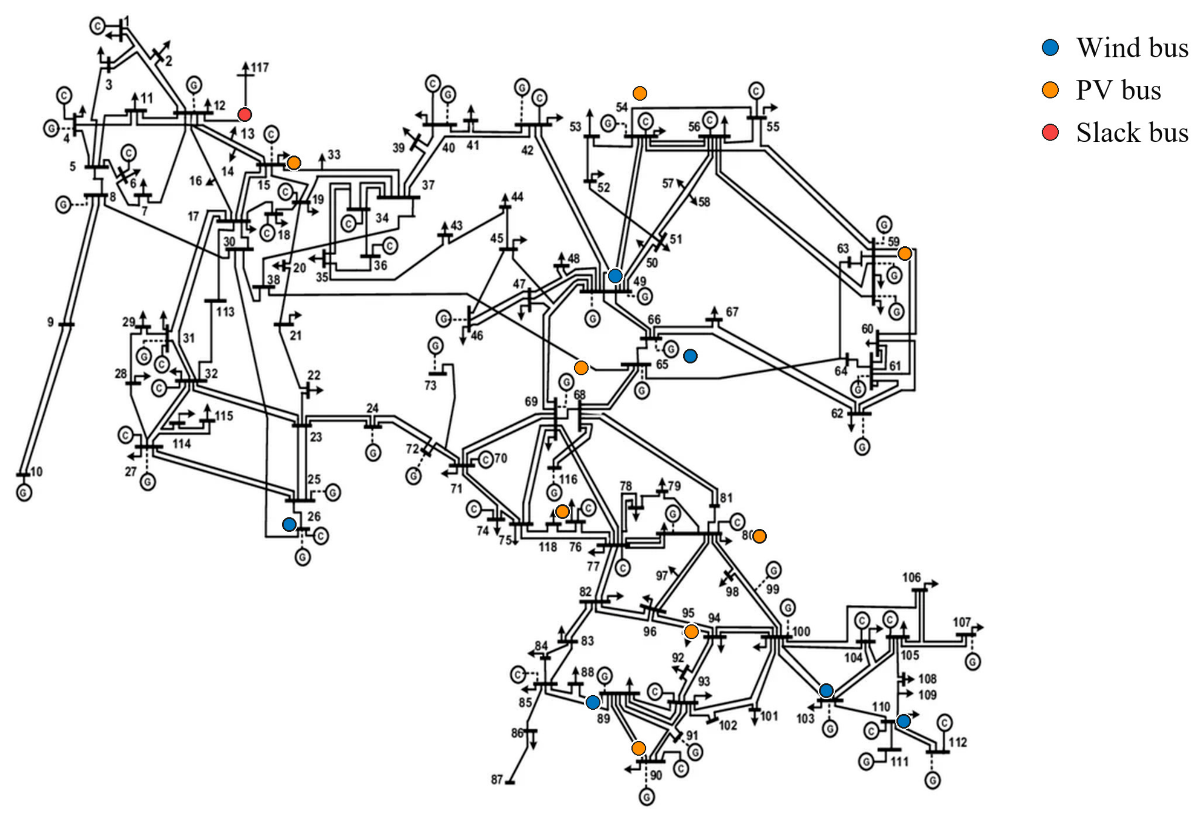
To evaluate the effectiveness of the proposed method for rapidly generating commitment schedules, case studies are conducted on a modified IEEE 118-bus system. Renewable sources are added to the original system, as shown in Figure 1. The case studies assess the proposed method in terms of operational feasibility, commitment schedule similarity, operating economy, and computational efficiency.

The system contains 54 conventional units, the total minimum and maximum outputs of which are 2334 MW and 8270 MW, respectively. Wind farms are connected at buses 26, 49, 65, 89, 103, and 110, with a total installed capacity of 3920.04 MW. PV stations are connected at buses 59, 68, 80, 54, 76, 90, 95, and 15, with a total installed capacity of 3584.60 MW. The total installed capacity of renewable energy is therefore 7504.64 MW.

The dataset contains 1821 operating days from 2 January 2015 to 31 December 2019. For each day, the scheduling horizon is 24 h with an hourly time resolution. The first 1456 days form the historical commitment schedule library, and the last 365 days are taken as the test set. The same split is applied for both the UC and the SCUC cases.

For each historical day, its standardized net-load trajectory, hourly unit commitment matrix, and operating cost are recorded. When generating the schedule, the load, wind power, and PV output of the target day are used to form a 24 h net-load trajectory, from which the Top-K most similar historical days are retrieved from the library. K is set to four in this paper.

The retrieved candidate commitment schedules are then fed one by one into the verification model with fixed binary variables. If no candidate satisfies strict feasibility, or candidates exhibit large cost deviations, the limited-perturbation repair model is applied to produce the final unit commitment schedules. The full UC and full SCUC solutions serve as the benchmark for evaluating the feasibility, commitment schedule similarity, and operating economy of the generated commitment schedule.

All optimization models are implemented with YALMIP 20250626 and solved by Gurobi 12.0.3 on a Windows workstation equipped with an Intel U7 265K processor and 32 GB of memory.

The evaluation metrics include strict feasibility rate, commitment schedule similarity, objective function deviation, and computation time.

The strict feasibility rate measures whether the generated schedule leads to a solution that satisfies all constraints during the subsequent fixed-binary verification or repair process. It is defined as shown in (41).

$$R_{\mathrm{fea}}={\displaystyle \frac{N_{\mathrm{fea}}}{N_{\mathrm{test}}}}\times 100\%$$

(41)

In (41), $R_{\mathrm{fea}}$ represents the strict feasibility rate. $N_{\mathrm{fea}}$ denotes the number of test days satisfying the strict feasibility criterion, and $N_{\mathrm{test}}$ denotes the total number of test days.

The commitment schedule similarity characterizes the consistency between the generated commitment matrix and the commitment matrix of the full UC benchmark. It is defined as (42).

$$S_u=\left(1-{\displaystyle \frac{{{\displaystyle \sum }}_{n=1}^N{{\displaystyle \sum }}_{t=1}^T\left|u_{n,t}^{\mathrm{gen}}-u_{n,t}^{\mathrm{UC}}\right|}{NT}}\right)\times 100\%$$

(42)

In (42), $S_u$ represents the commitment schedule similarity. $u_{n,t}^{\mathrm{gen}}$ denotes the ON/OFF statuses of unit $n$ at hour $t$ generated by the proposed method; $NT=N\times T$ is the total number of unit-hour statuses; and $u_{n,t}^{\mathrm{UC}}$ denotes the corresponding ON/OFF statuses obtained from the full UC benchmark model.

The objective function deviation reflects the economic loss of the generated schedule relative to the full UC benchmark. It is defined as (43).

$$G_F=\left|{\displaystyle \frac{F^{\mathrm{gen}}-F^{\mathrm{UC}}}{F^{\mathrm{UC}}}}\right|\times 100\%$$

(43)

In (43), $G_F$ represents the objective function deviation. $F^{\mathrm{gen}}$ denotes the operating cost obtained after the verification with fixed binary variables dispatch or repair of the generated commitment schedule, and $F^{\mathrm{UC}}$ denotes the optimal operating cost of the full UC.

Intuitively, a larger $R_{\mathrm{fea}}$ represents a higher feasibility rate; an $S_u$ value closer to 100% represents stronger consistency with the benchmark commitment schedule, and a $G_F$ value closer to zero represents a smaller operating-cost deviation from the benchmark.

4.2. Performance Comparison with UC and SCUC Cases

(i)

Results for the UC case

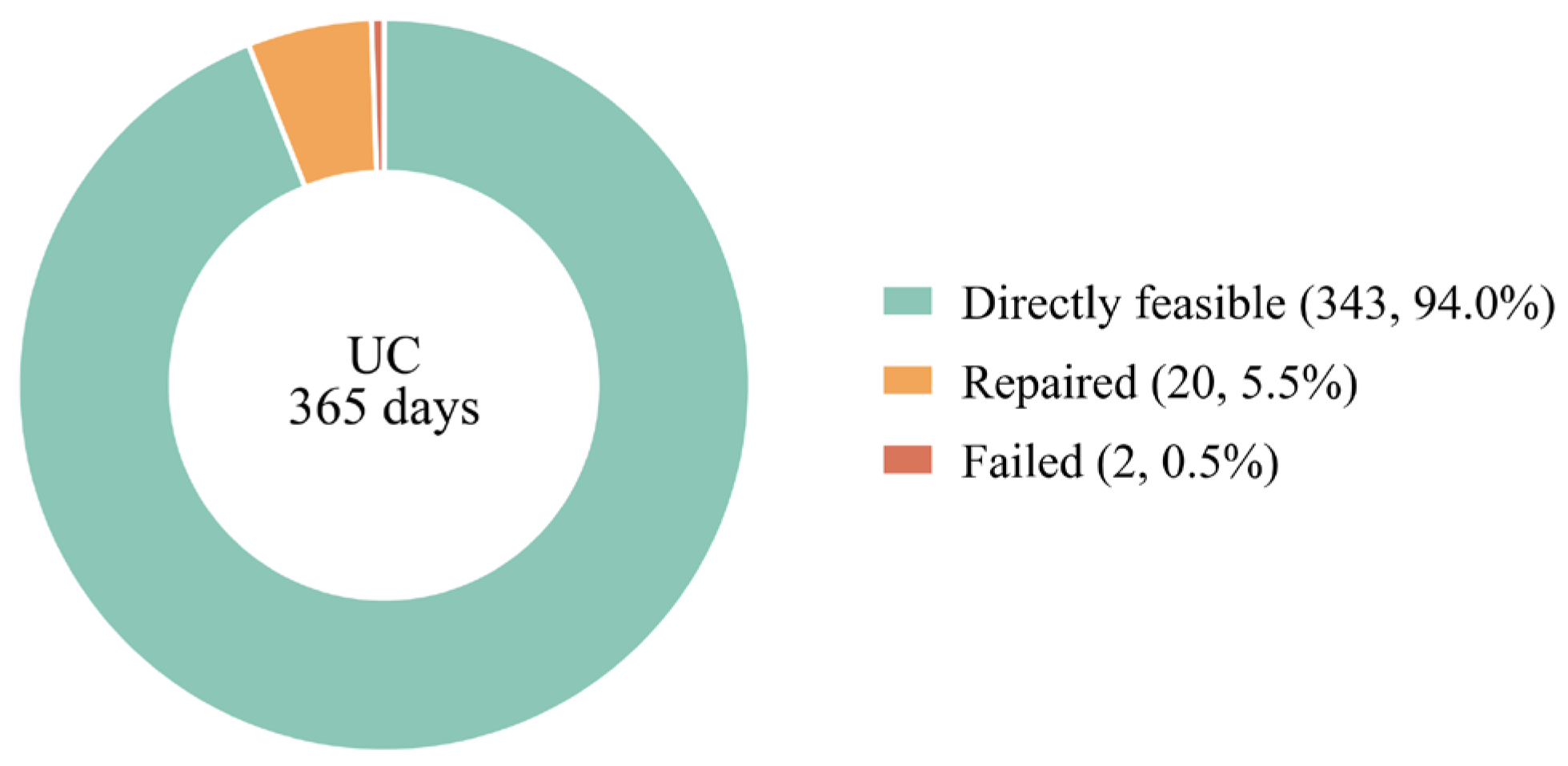
The UC case results are first analyzed to evaluate the performance of the proposed method. As shown in Figure 2 and

Table 1. Summary of the UC case results.

Index	Result
Generation outcome	343 direct; 20 repaired; 2 failed
Successful generation rate	99.45%
Objective function deviation	mean 0.522%; median 0.225%; 95th percentile 2.465%
Schedule similarity	mean 96.3%; median 97.1%; 95th percentile 98.9%
Computation time	proposed 2.10 s/day; full UC 11.09 s/day

, commitment schedules for most UC test days can be directly generated. For most test days, the final commitment schedule is selected directly from the Top-4 candidates, and all four candidates are strictly feasible in many cases. Among the test days, 266 days have all four strictly feasible candidates in the Top-4 set, indicating that net-load trajectory similarity-based retrieval could provide a sufficiently rich candidate set for most UC operating conditions.

Among the 365 UC test days, feasible solutions are obtained directly from the retrieved candidates for 343 days, while the limited-perturbation repair successfully handles another 20 days, leaving only two unsuccessful cases. The two unsuccessful days have standardized distances greater than 1.9, compared with an average distance of 1.4 for the successfully generated days. Both unsuccessful cases correspond to extreme low-net-load and high-renewable conditions, with net loads falling within the lowest 4% of the test set. Neither case has a close neighbor in the historical library, suggesting that the failures are associated with insufficient library coverage of these extreme operating conditions. The commitment schedules generated also remain close to benchmark schedules obtained by solving the full UC model, with a mean objective function deviation of 0.522%, a median deviation of 0.225%, and a 95th percentile deviation of 2.465%. The mean schedule similarity reaches 96.3%, further showing that the proposed method can preserve the main commitment schedule of the benchmark UC solution.

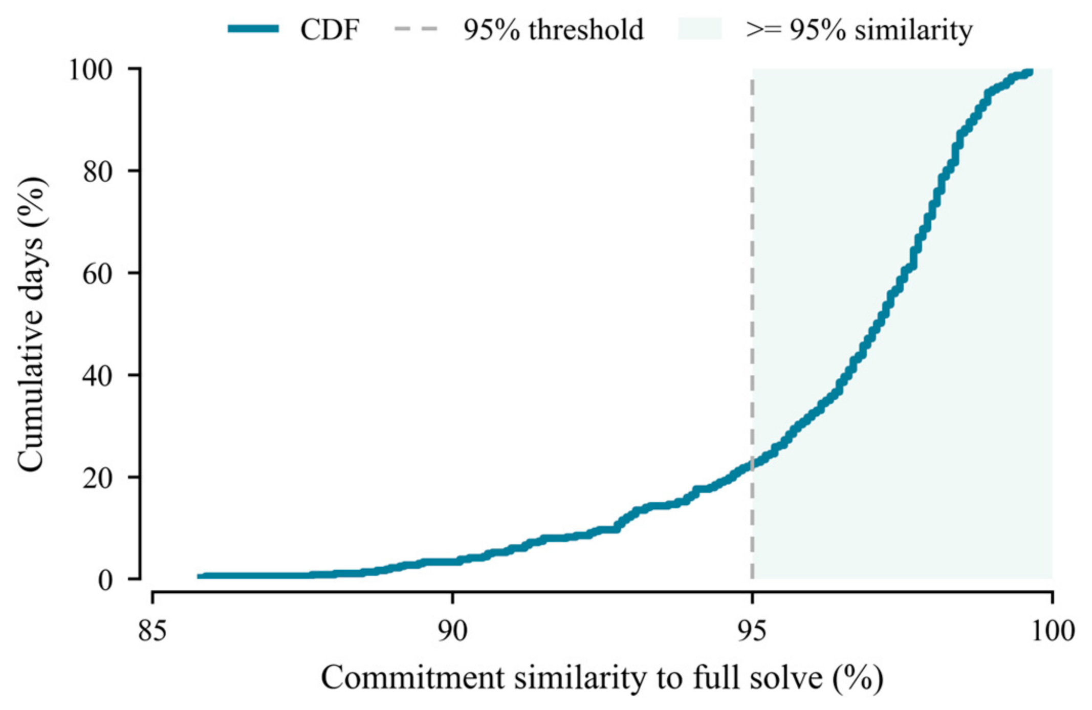
To further evaluate the share of test days with generated schedules that are close to the full UC benchmark, Figure 3 presents the cumulative distribution of the commitment schedule similarity between the generated schedules and the full UC benchmark. As shown in Figure 3, only about 20% of the test days fall below the 95% similarity threshold, while the majority of days achieve higher similarity. This shows that the proposed method reproduces the benchmark commitment schedule and changes only a few unit statuses.

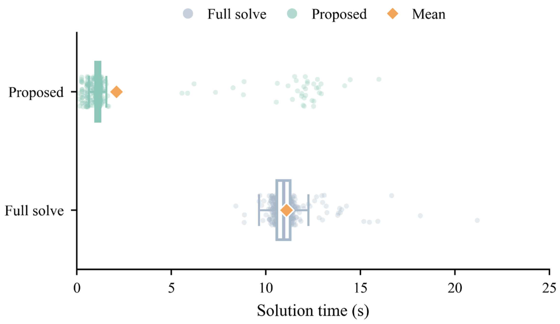
To further compare the computational efficiency of the proposed method and the full UC benchmark, Figure 4 presents the distribution of daily solution time over all test days. As shown in Figure 4, the proposed method generally requires less solution time than the full UC model, and its solution-time distribution is concentrated in a lower range. Although a few days require additional time due to repair, the average computation time of the proposed method remains much lower than that of solving the full UC benchmark.

To assess whether the time reduction is statistically meaningful, the computation times are compared statistically in

Table 2. Statistical comparison of the computation time in the UC case.

Method	Mean (s/Day)	Standard Deviation (s)	95% Confidence Interval (s/Day)
Full UC	11.09	1.07	[10.98, 11.20]
Proposed	2.10	3.27	[1.76, 2.44]

. The 95% confidence intervals of the two methods are far apart, so the difference cannot be attributed to random fluctuations across days. The proposed method also has a larger standard deviation than the full solve, because most days are generated directly from the retrieved candidates and only a few require the repair model, which produces a small number of slower days rather than a longer computation time. Even so, the proposed method is faster on 93.7% of the test days, which confirms that the advantage persists across individual test days rather than only on average. The difference is further confirmed by a paired Wilcoxon signed-rank test, a non-parametric test that compares the per-day computation times of the two methods without assuming a normal distribution. The test rejects the hypothesis of equal computation time (p < 0.001).

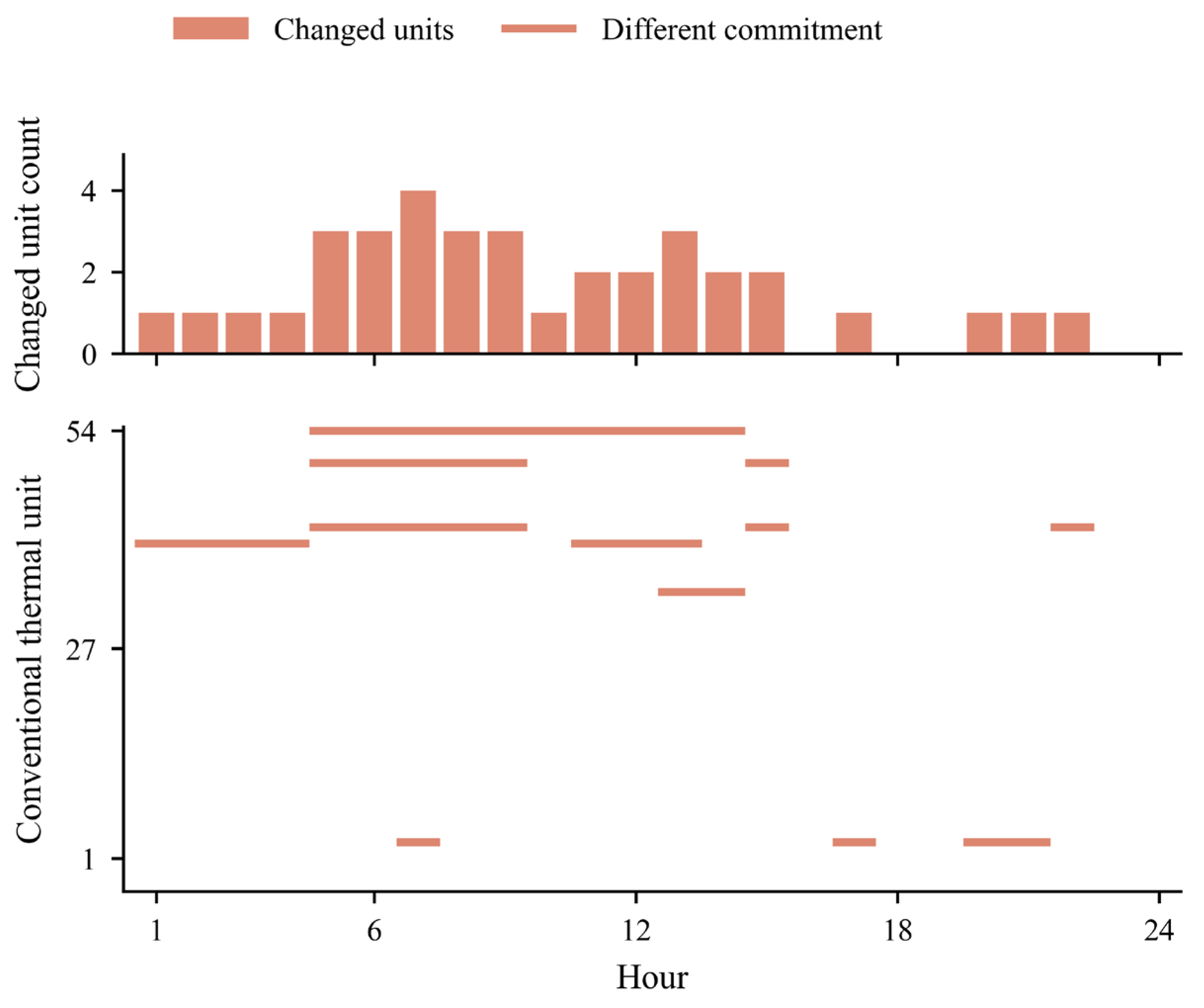
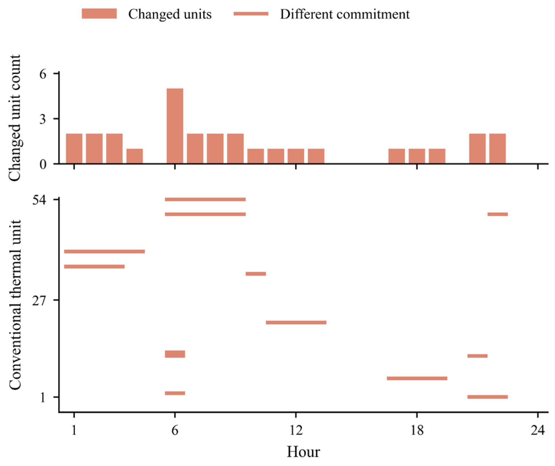
As illustrated in Figure 5, the commitment schedule generated differs only slightly from the full UC benchmark for a small number of units and hours. This suggests that the retrieved historical schedule already provides a close match for the target day, and only minor adjustments are needed in the final generated schedule if necessary.

(ii)

Results for the SCUC case

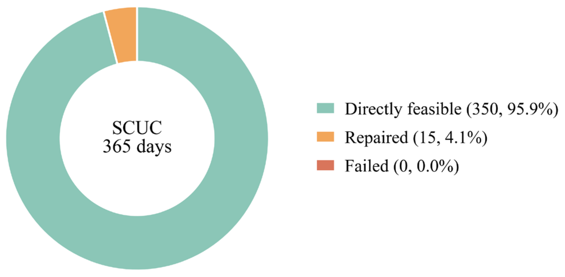
The SCUC case results are then analyzed to evaluate the performance of the proposed method. As shown in Figure 6 and

Table 3. Summary of the SCUC case results.

Index	Result
Generation outcome	350 direct; 15 repaired; 0 failed
Successful generation rate	100%
Objective function deviation	mean 0.558%; median 0.217%; 95th percentile 2.782%
Schedule similarity	mean 95.3%; median 96.1%; 95th percentile 98.5%
Computation time	proposed 32.18 s/day; full SCUC 63.48 s/day

, the proposed method also maintains a high successful generation rate in the SCUC case. Although additional network security constraints are considered, 290 days still have four strictly feasible candidates in the Top-4 set. This shows that the historical commitment schedule retrieval mechanism remains effective under security-constrained operation.

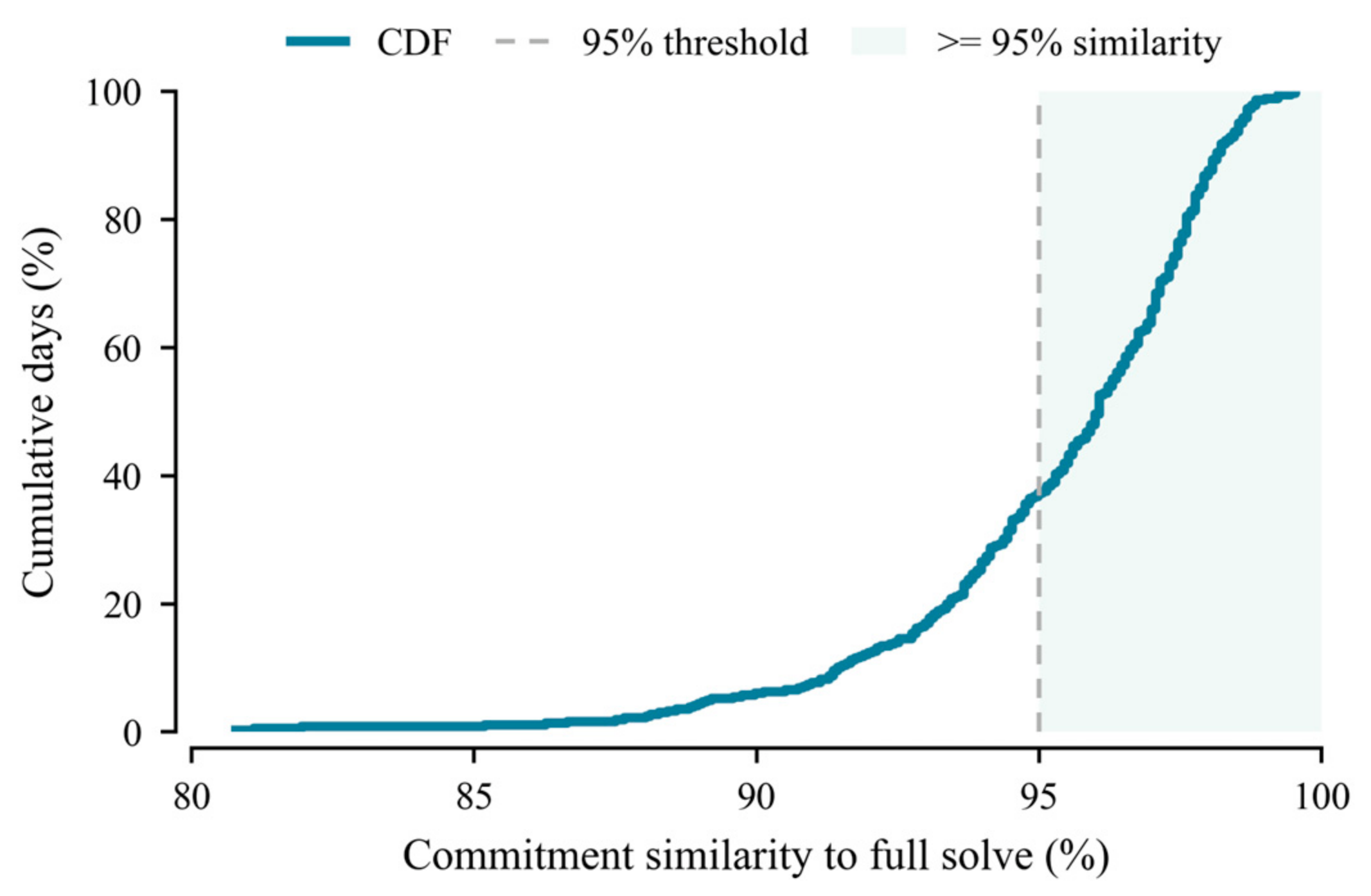
The similarity distribution in Figure 7 is concentrated in the high-value range, which means, in general, that the generated schedules closely match the full SCUC benchmark for most test days. This result suggests that, even with network security constraints, the proposed method can reproduce the main unit ON/OFF patterns of the full SCUC solution through historical schedule transfer and limited repair.

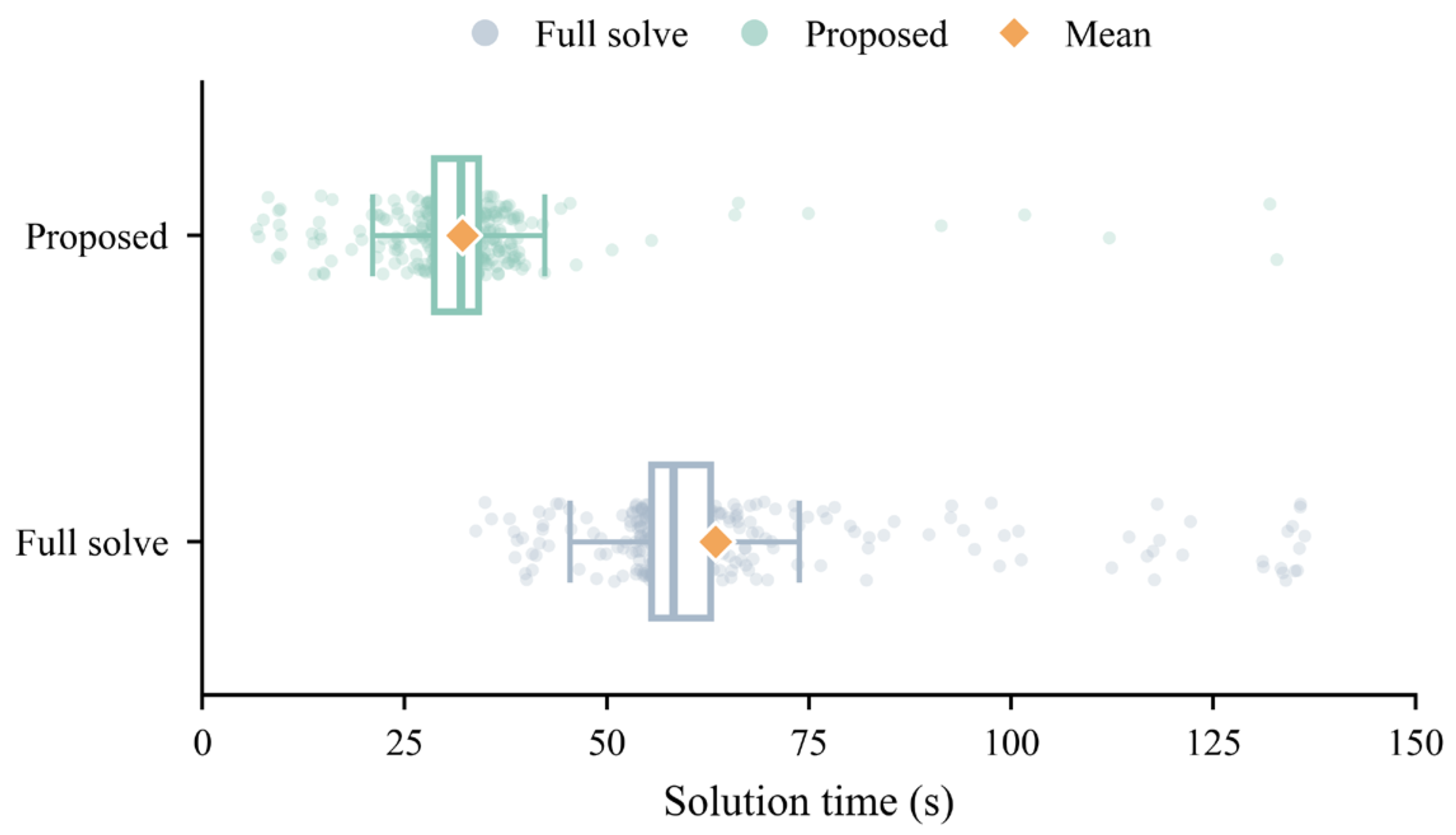
Compared with the UC case, in the SCUC case, the proposed method shows a clear computational advantage. As shown in Figure 8, the computation time distribution of the proposed method shifts left relative to the full SCUC benchmark.

The same statistical comparison is made for the SCUC case in

Table 4. Statistical comparison of the computation time in the SCUC case.

Method	Mean (s/Day)	Standard Deviation (s)	95% Confidence Interval (s/Day)
Full SCUC	63.48	18.98	[61.53, 65.43]
Proposed	32.18	12.30	[30.92, 33.44]

. The full SCUC solve is not only slower but also substantially more variable, with a standard deviation of 18.98 s, because its solution time depends strongly on the difficulty of the security-constrained MILP for each day. Fixing the commitment variables removes most of this variability, so the proposed method is both faster and more predictable, which is desirable when many scenarios must be evaluated within a limited time. The proposed method is faster on 98.9% of the test days, showing that the advantage is consistent across the whole test set. The paired Wilcoxon signed-rank test on the computation times leads to the same conclusion for the SCUC case (p < 0.001).

The computational advantage mainly comes from two aspects. First, the verification model fixes the unit commitment variables. Second, the limited-perturbation repair model is activated only for a limited number of test days, so its additional computational cost remains low.

Figure 9 shows that the commitment schedule generated in an SCUC case differs from the full SCUC solution only for a small number of units and hours. This indicates that the proposed method preserves most of the retrieved historical schedule while making only limited adjustments.

4.3. Sensitivity and Ablation Analysis

To further examine the behavior of the proposed method, this subsection studies the effect of the retrieval size, namely K, the choice of similarity metric, the contribution of each pipeline component, the repair penalty, and the robustness over different data partitions.

(i)

Effect of the retrieval size K

The retrieval size K determines how many historical candidates are verified for each target day. As shown in

Table 5. Effect of the retrieval size K.

K	UC SGR	UC Mean Cost Deviation	UC Time (s/Day)	SCUC SGR	SCUC Mean Cost Deviation	SCUC Time (s/Day)
1	98.90%	0.712%	1.3	99.73%	0.860%	10.2
2	99.18%	0.569%	1.7	100%	0.641%	15.6
3	99.18%	0.549%	1.9	100%	0.588%	24.7
4	99.45%	0.522%	2.1	100%	0.558%	32.2
6	99.45%	0.600%	2.8	100%	0.562%	43.1
8	99.45%	0.614%	3.5	100%	0.571%	60.1

, the UC successful generation rate (SGR) increases with K and reaches 99.45% at K = 4, while the SCUC rate reaches 100% from K = 2. The mean cost deviation is lowest with K = 4 in both cases and does not improve for larger K, whereas the computation time keeps growing with K. Larger values of K are unnecessary, since they add computation without improving feasibility or economy.

(ii)

Choice of similarity metric

We compared the Euclidean distance with four alternative measures, including cosine, correlation, Mahalanobis distance, and DTW. The results are summarized in

Table 6. Comparison of similarity metrics.

Metric	UC Median Deviation	UC 95th-Pct Deviation	SCUC Median Deviation	SCUC 95th-Pct Deviation
Euclidean	0.225%	2.47%	0.217%	2.78%
Cosine	0.343%	7.97%	0.383%	6.90%
Correlation	0.492%	16.62%	0.433%	15.78%
Mahalanobis	0.675%	13.14%	0.627%	9.78%
DTW	0.320%	3.65%	0.288%	4.41%

.

The retrieval methods based on cosine, correlation, and Mahalanobis distances achieve a 100% SGR, but increase the 95th-percentile cost deviation to 6.9–17%, while that of the Euclidean distance is about 2.5%. This is because they match the shape of the net-load curve while ignoring its magnitude. DTW brings no improvement under the fixed 24 h alignment. The Euclidean distance therefore gives the lowest cost deviation, which supports its use in the proposed method.

(iii)

Component-wise ablation

Table 7. Ablation study of the pipeline components (UC case).

Variant	SGR	Mean Deviation
Full method	99.45%	0.522%
Without Top-K (K = 1)	98.90%	0.712%
Without repair	93.97%	—
Without standardization	99.45%	0.585%
Without redundancy removal	99.45%	0.687%

reports an ablation study in which each module is disabled in turn. Removing the Top-K mechanism (K = 1) lowers the SGR from 99.45% to 98.90% and raises the mean deviation from 0.522% to 0.712%. Disabling the repair model has the largest effect, reducing the SGR to 93.97%, which shows that repair recovers about 5% of the days. Removing the hour-wise standardization or the redundancy removal increases the mean deviation to 0.585% and 0.687%, respectively. This is because these two steps also affect the economy of the retrieved candidates. Standardization keeps the distance from being dominated by high-load hours, and redundancy removal keeps the candidate library small and avoids retrieving several near-identical schedules.

(iv)

Comparison with the CVAE-based generation

To compare with a learning-based alternative, a conditional variational autoencoder (CVAE), a deep generative model that learns to produce commitment schedules from the daily load, wind, and PV trajectories, is trained on the same historical library (2015–2018) and tested on the same 365 days of 2019. The CVAE samples twenty candidate schedules per day, which are verified and repaired by the same pipeline as the proposed method. As shown in

Table 8. Comparison with the CVAE-based generation (UC case).

Method	SGR	Mean Deviation	95th-Pct Deviation	Computation Time
Proposed	99.45%	0.522%	2.47%	2.10 s/day
CVAE	100%	0.846%	3.93%	7.01 s/day

, the CVAE reaches a similar successful-generation rate, but its mean and 95th-percentile cost deviations are clearly larger.

4.4. Discussion and Limitations

The present cases evaluate previously unseen operating days under a fixed system configuration, since the 2019 test days are excluded from the 2015–2018 historical library. The two unsuccessful UC cases further show that insufficient historical coverage can limit performance when the target operating condition differs substantially from those represented in the library. It is worthwhile to mention that changes in generation portfolios and network configurations are not tested in this work. The strategies discussed below therefore provide general guidance for handling these situations.

It should be noted that the numerical validation in this study is limited to the modified IEEE 118-bus system, and the reported results should therefore be interpreted within this scope. The proposed framework nevertheless has a computationally simple retrieval stage based on distance calculations between 24 h net-load trajectories, while the candidate verification fixes the commitment-related binary variables and reduces the original UC or SCUC problem to an LP. The repair model is required only for a small fraction of cases, although it remains an MILP when activated. These characteristics explain the computational improvement observed in the present case studies, but do not by themselves constitute a general scalability assessment.

5. Conclusions

This paper proposes a fast UC and SCUC schedule generation method based on standardized net-load trajectory similarity and historical schedule transfer. For a target day, Top-K historical schedules with similar net-load trajectories are retrieved as candidates, verified with fixed binary variables, and repaired through limited perturbation when necessary. Case studies on the modified IEEE 118-bus system show that the proposed method can generate feasible commitment schedules with small economic deviations. For the tested system, the successful generation rates reach 99.45% in the UC case and 100% in the SCUC case. The mean objective function deviations are 0.522% and 0.558%, and the mean commitment schedule similarities are 96.3% and 95.3%, respectively. In the SCUC case, the average computation time is reduced from 63.48 s/day to 32.18 s/day, achieving a speedup of 1.97 times. These results show that the proposed method can effectively reuse historical commitment structures on the tested system while maintaining feasibility, economic performance, and computational efficiency. Nevertheless, two UC test days remain unsuccessful, indicating that a full UC solve is still necessary as a fallback under extreme operating conditions. In addition, the current validation is limited to the modified IEEE 118-bus system with a fixed system configuration. Therefore, the scalability of the proposed method to larger systems, as well as its adaptability to changing generation portfolios, dynamically updated historical libraries, and other power systems, remains to be further investigated.

References

1. Howlader, H.O.R.; Sediqi, M.M.; Ibrahimi, A.M.; Senjyu, T. Optimal thermal unit commitment for solving duck curve problem by introducing CSP, PSH and demand response. IEEE Access 2018, 6, 4834–4844. [Google Scholar] [CrossRef] [Scilit]
2. Chen, Y.; Pan, F.; Qiu, F.; Xavier, A.S.; Zheng, T.; Marwali, M.; Knueven, B.; Guan, Y.; Luh, P.B.; Wu, L.; et al. Security-constrained unit commitment for electricity market: Modeling, solution methods, and future challenges. IEEE Trans. Power Syst. 2023, 38, 4668–4681. [Google Scholar] [CrossRef] [Scilit]
3. Tejada-Arango, D.A.; Lumbreras, S.; Sánchez-Martín, P.; Ramos, A. Which unit-commitment formulation is best? A comparison framework. IEEE Trans. Power Syst. 2020, 35, 2926–2936. [Google Scholar] [CrossRef] [Scilit]
4. Li, H.; Ren, Z.; Fan, M.; Li, W.; Xu, Y.; Jiang, Y.; Xia, W. A review of scenario analysis methods in planning and operation of modern power systems: Methodologies, applications, and challenges. Electr. Power Syst. Res. 2022, 205, 107722. [Google Scholar] [CrossRef] [Scilit]
5. Zheng, K.; Sun, Z.; Song, Y.; Zhang, C.; Zhang, C.; Chang, F.; Yang, D.; Fu, X. Stochastic scenario generation methods for uncertainty in wind and photovoltaic power outputs: A comprehensive review. Energies 2025, 18, 503. [Google Scholar] [CrossRef] [Scilit]
6. Chen, Y.; Wang, Y.; Kirschen, D.S.; Zhang, B. Model-free renewable scenario generation using generative adversarial networks. IEEE Trans. Power Syst. 2018, 33, 3265–3275. [Google Scholar] [CrossRef] [Scilit]
7. Dong, W.; Chen, X.; Yang, Q. Data-driven scenario generation of renewable energy production based on controllable generative adversarial networks with interpretability. Appl. Energy 2022, 308, 118387. [Google Scholar] [CrossRef] [Scilit]
8. Dalal, D.; Bilal, M.; Shah, H.; Sifat, A.I.; Pal, A.; Augustin, P. Cross-correlated scenario generation for renewable-rich power systems using implicit generative models. Energies 2023, 16, 1636. [Google Scholar] [CrossRef] [Scilit]
9. Gao, Y.; Dong, H.; Hu, L.; Lin, Z.; Zeng, F.; Ye, C.; Zhang, J. A morphing-based future scenario generation method for stochastic power system analysis. Sustainability 2024, 16, 2762. [Google Scholar] [CrossRef] [Scilit]
10. Ma, T.; Qin, B.; Hong, S.; Su, Y. Mathematical analysis methods for quantitative scenario generation of renewable power output: A comprehensive review. Energies 2026, 19, 1701. [Google Scholar] [CrossRef] [Scilit]
11. Wu, J.; Luh, P.B.; Chen, Y.; Yan, B.; Bragin, M.A. Synergistic integration of machine learning and mathematical optimization for unit commitment. IEEE Trans. Power Syst. 2023, 39, 391–401. [Google Scholar] [CrossRef] [Scilit]
12. Gao, Q.; Yang, Z.; Li, W.; Yu, J.; Lu, Y. Online learning of stable integer variables in unit commitment using internal information. IEEE Trans. Power Syst. 2023, 38, 2947–2950. [Google Scholar] [CrossRef] [Scilit]
13. Porras, Á.; Pineda, S.; Morales, J.M.; Jimenez-Cordero, A. Cost-driven screening of network constraints for the unit commitment problem. IEEE Trans. Power Syst. 2022, 38, 42–51. [Google Scholar] [CrossRef] [Scilit]
14. Xavier, Á.S.; Qiu, F.; Ahmed, S. Learning to solve large-scale security-constrained unit commitment problems. INFORMS J. Comput. 2021, 33, 739–756. [Google Scholar] [CrossRef] [Scilit]
15. Gasse, M.; Chételat, D.; Ferroni, N.; Charlin, L.; Lodi, A. Exact combinatorial optimization with graph convolutional neural networks. In Proceedings of the 33rd Conference on Neural Information Processing Systems (NeurIPS 2019), Vancouver, BC, Canada, 8–14 December 2019; Volume 32. [Google Scholar]
16. Khalil, E.; Le Bodic, P.; Song, L.; Nemhauser, G.; Dilkina, B. Learning to branch in mixed integer programming. In Proceedings of the AAAI Conference on Artificial Intelligence, Phoenix, AZ, USA, 12–17 February 2016; Volume 30. [Google Scholar]
17. Yurdakul, O.; Qiu, F.; Meyer, A. A predictive prescription framework for stochastic unit commitment using boosting ensemble learning algorithms. IEEE Trans. Power Syst. 2023, 39, 5726–5740. [Google Scholar] [CrossRef] [Scilit]
18. Wei, L.; Ai, X.; Fang, J.; Cui, S.; Gao, L.; Li, K.; Wen, J. Data-augmentation acceleration framework by graph neural network for near-optimal unit commitment. Appl. Energy 2025, 377, 124332. [Google Scholar] [CrossRef] [Scilit]
19. Ramesh, A.V.; Li, X. Feasibility layer aided machine learning approach for day-ahead operations. IEEE Trans. Power Syst. 2023, 39, 1582–1593. [Google Scholar] [CrossRef] [Scilit]
20. Venkatesh, B.; Shekeew, M.I.A.; Ma, J. Feasibility-guaranteed machine learning unit commitment: Fuzzy Optimization approaches. Appl. Energy 2025, 379, 124923. [Google Scholar] [CrossRef] [Scilit]
21. Berthold, M.R.; Höppner, F. On clustering time series using euclidean distance and pearson correlation. arXiv 2016, arXiv:1601.02213. [Google Scholar]
Figure 1. The modified IEEE 118-bus system.
Processes 14 02760 g001
Figure 2. Feasibility composition of generated commitment schedules in the UC case.
Processes 14 02760 g002
Figure 3. Cumulative distribution of commitment schedule similarity in the UC case.
Processes 14 02760 g003
Figure 4. Distribution of computation time in the UC case.
Processes 14 02760 g004
Figure 5. Unit commitment differences between the generated and benchmark schedules in a typical UC case.
Processes 14 02760 g005
Figure 6. Feasibility composition of generated commitment schedules in the SCUC case.
Processes 14 02760 g006
Figure 7. Cumulative distribution of commitment schedule similarity in the SCUC case.
Processes 14 02760 g007
Figure 8. Distribution of computation time in the SCUC case.
Processes 14 02760 g008
Figure 9. Unit commitment differences between the generated and benchmark schedules in a typical SCUC case.
Processes 14 02760 g009