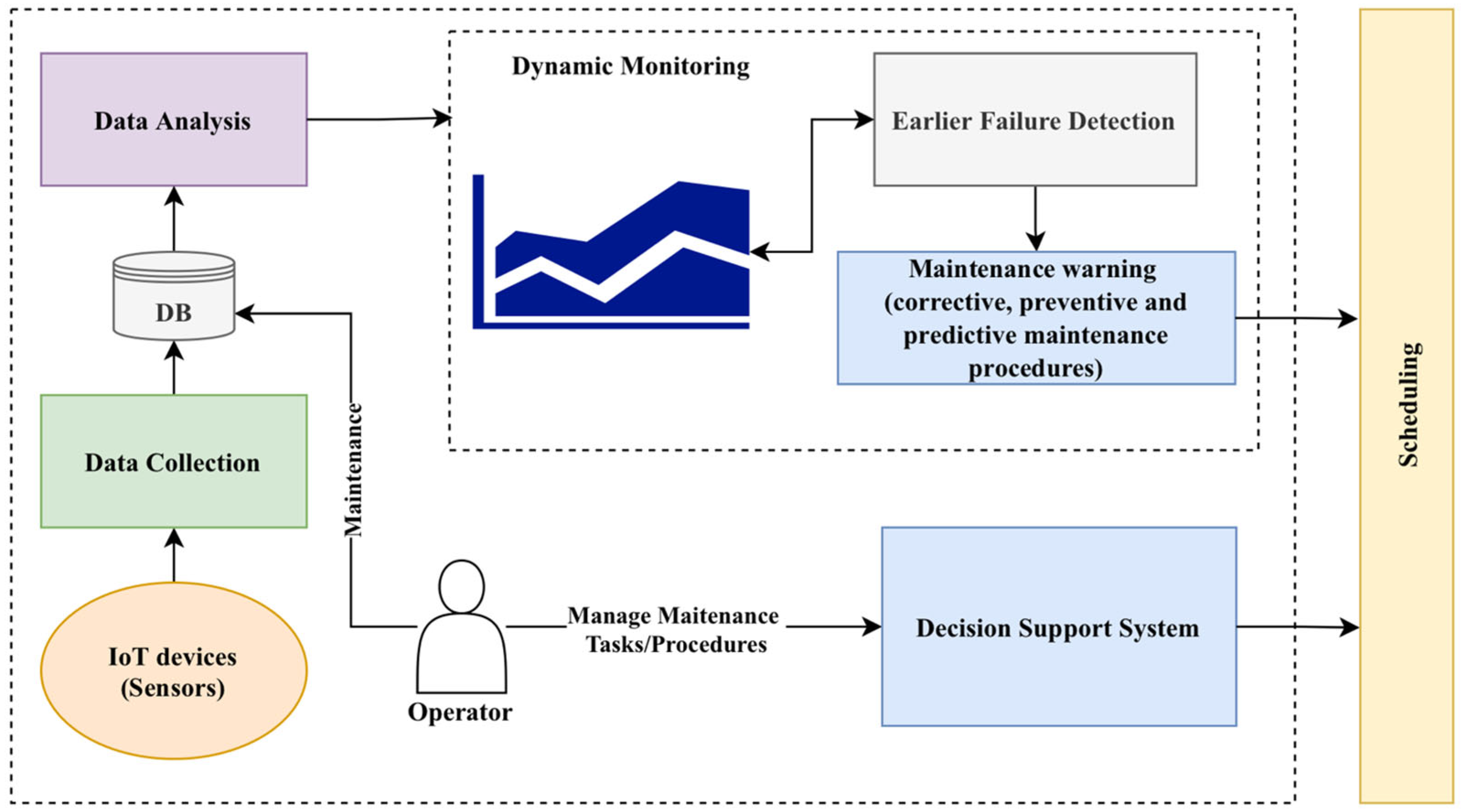
Figure 1.
Industry 4.0-based predictive maintenance system.
Figure 1.
Industry 4.0-based predictive maintenance system.
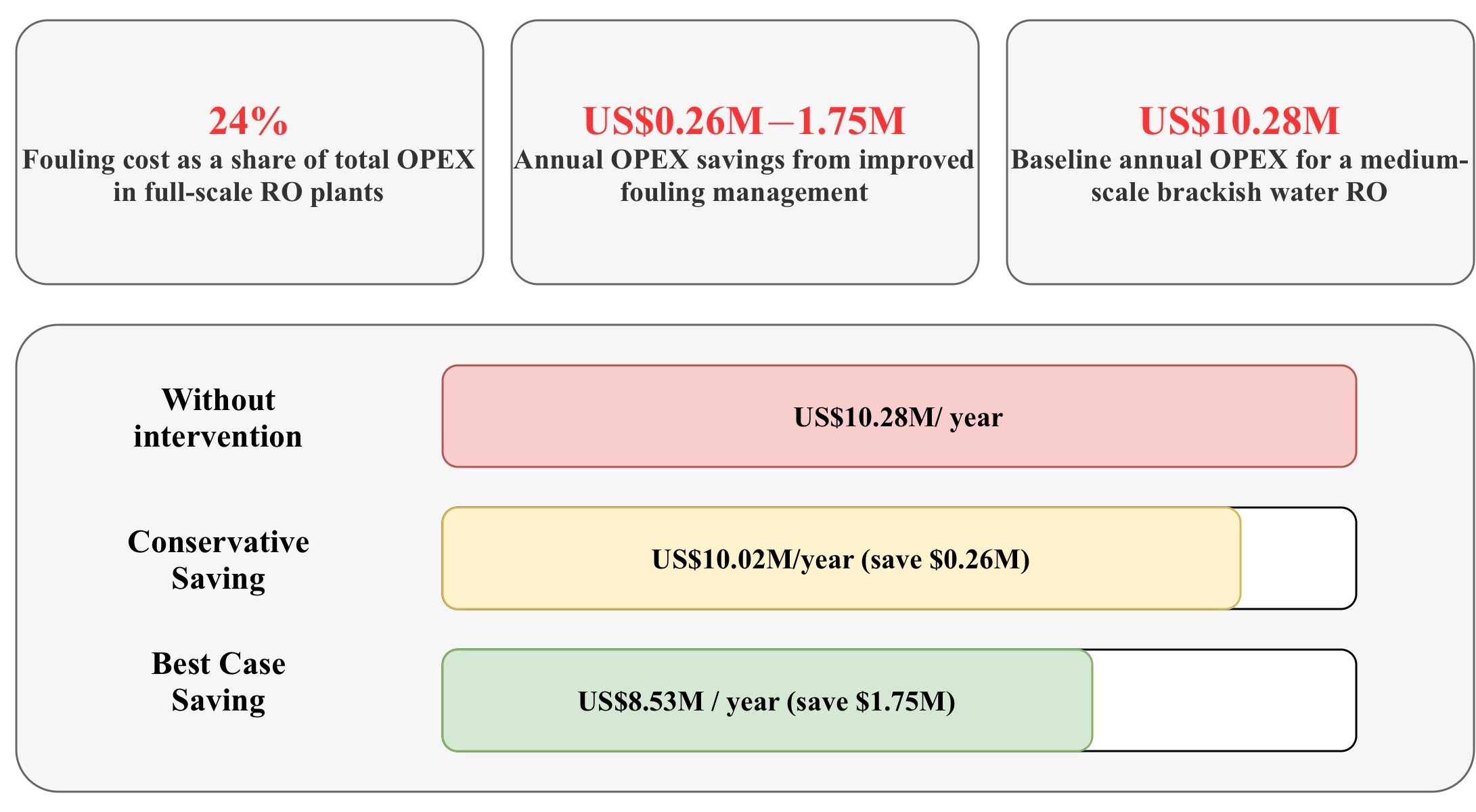
Figure 2.
Economic impact of membrane fouling in RO water treatment operations.
Figure 2.
Economic impact of membrane fouling in RO water treatment operations.
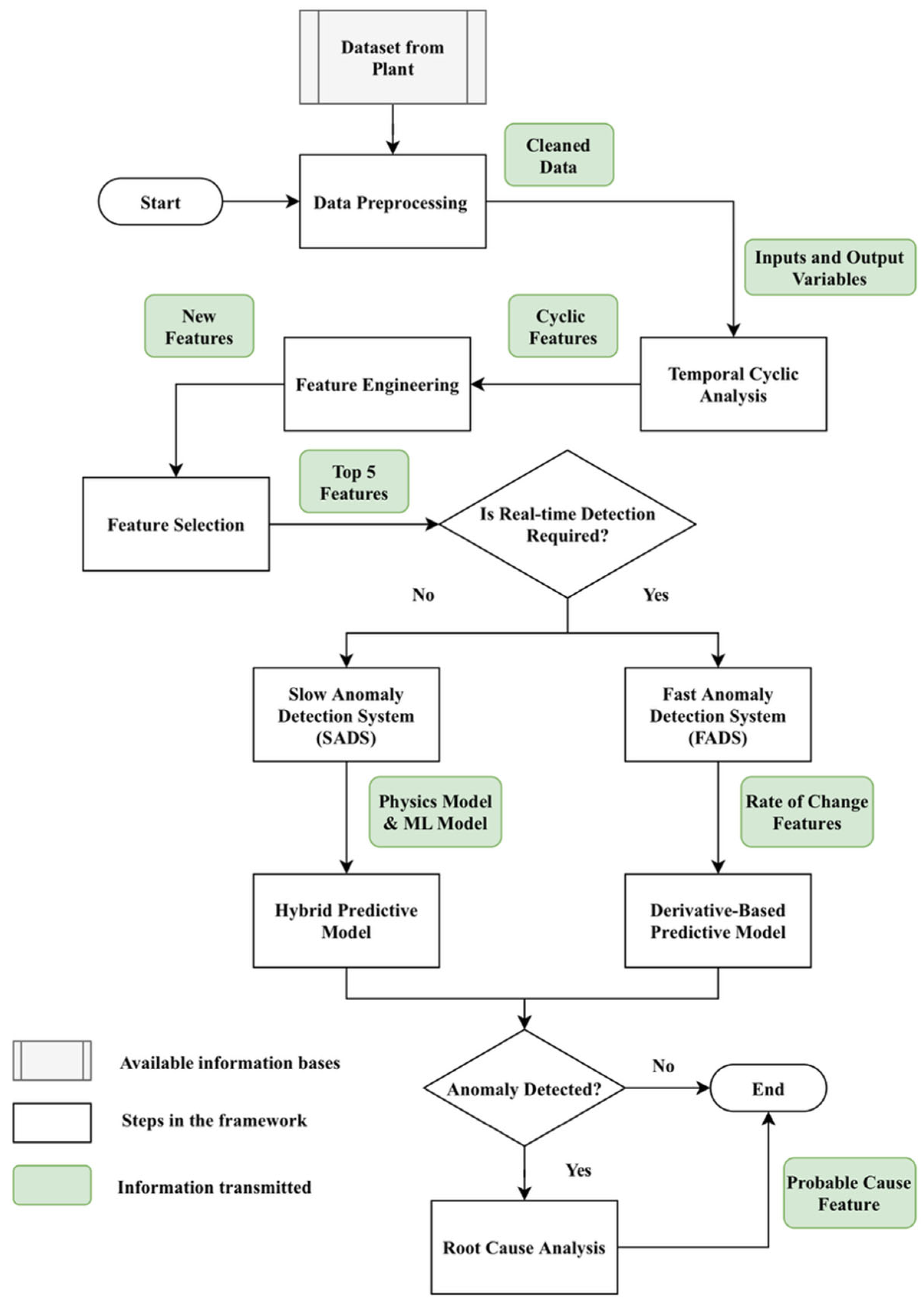
Figure 3.
Proposed generic framework.
Figure 3.
Proposed generic framework.
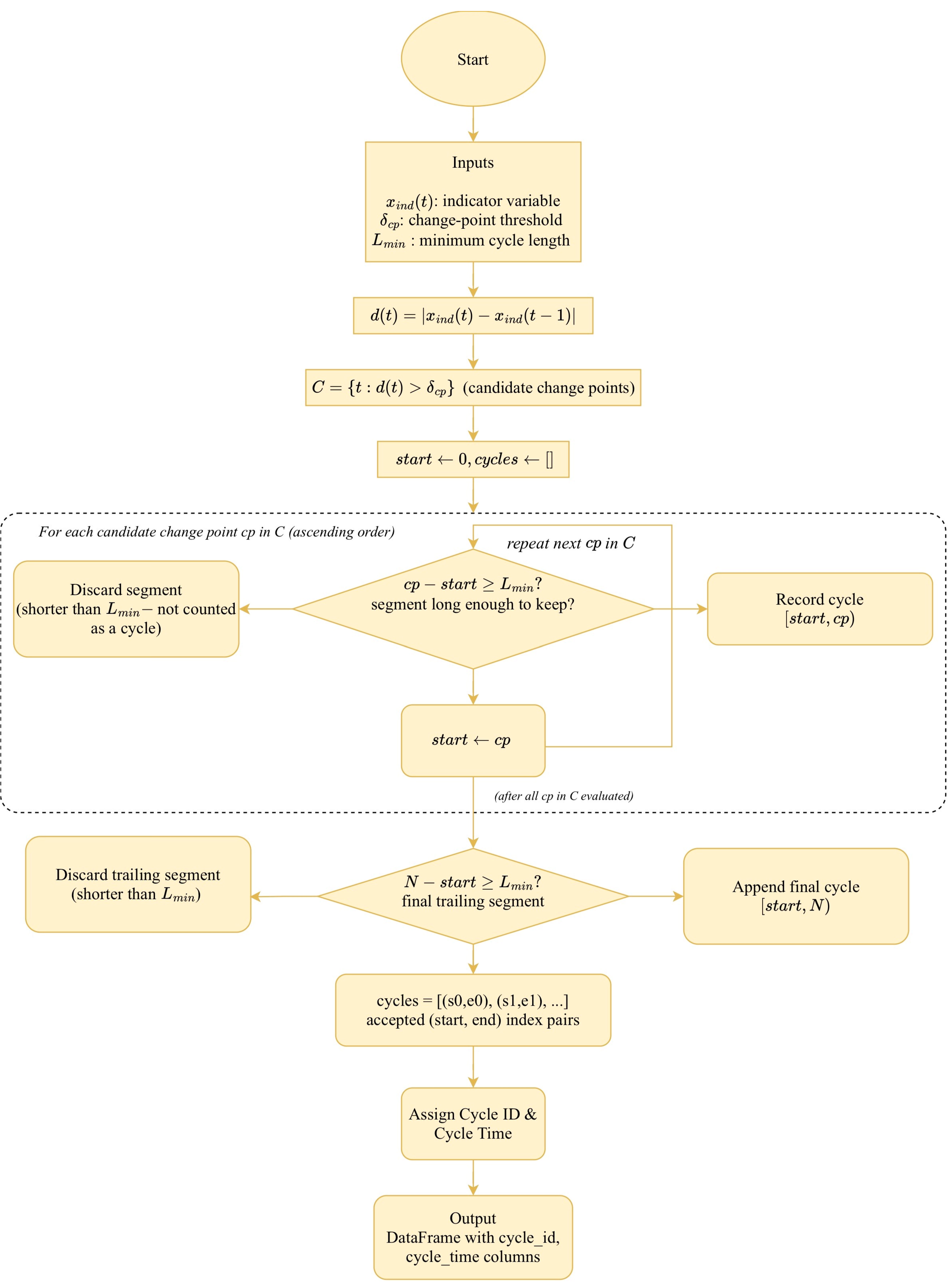
Figure 4.
Pictorial algorithm of temporal cyclic analysis.
Figure 4.
Pictorial algorithm of temporal cyclic analysis.
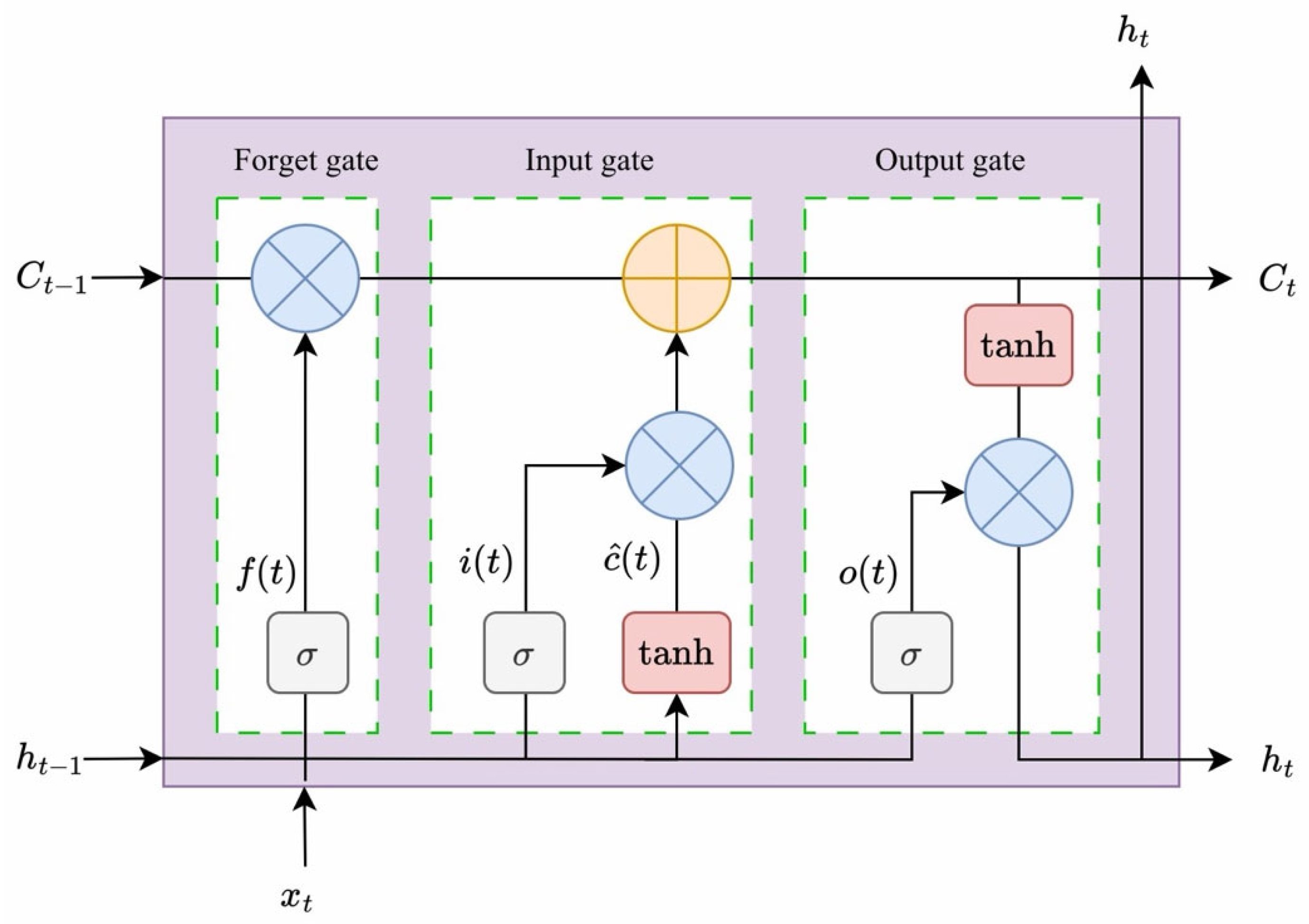
Figure 5.
LSTM architecture.
Figure 5.
LSTM architecture.
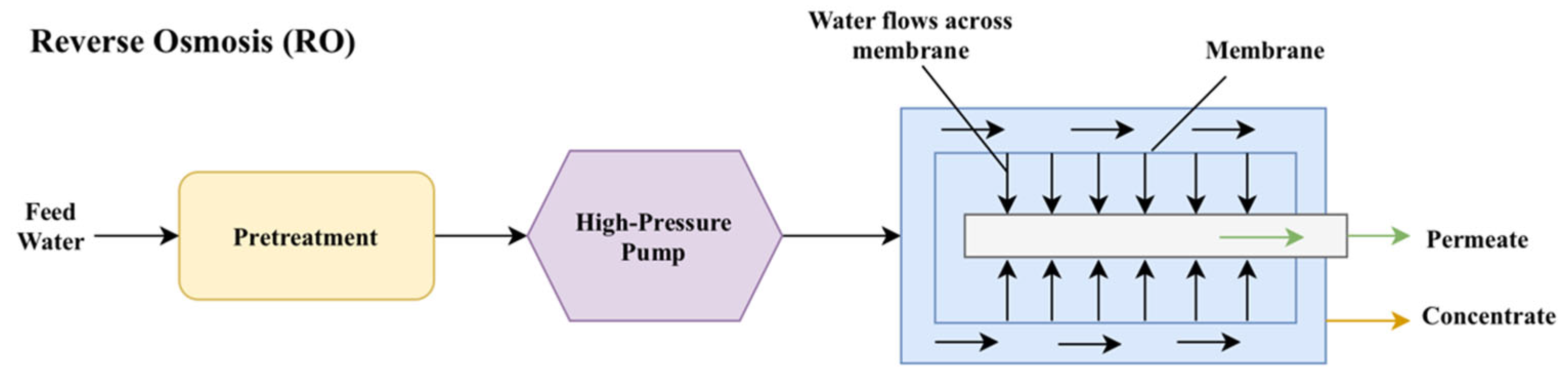
Figure 6.
A schematic of the RO system.
Figure 6.
A schematic of the RO system.
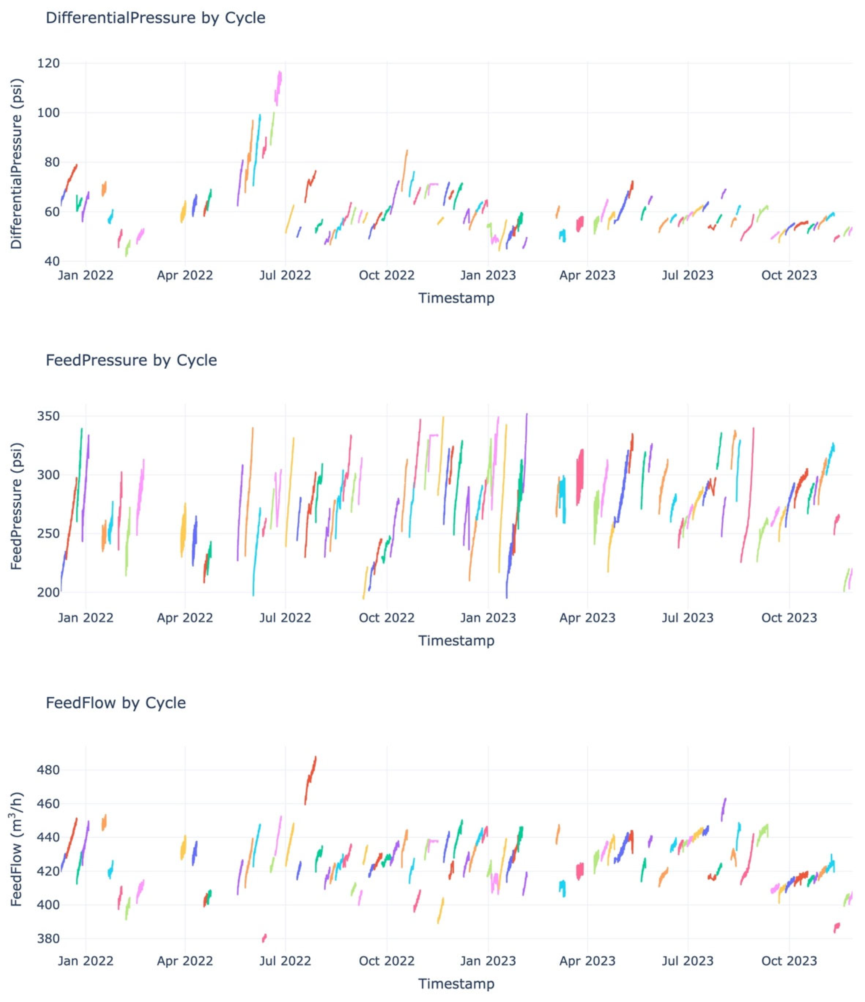
Figure 7.
Cycle distributions of Differential Pressure, Feed Pressure, and Feed Flow on a 1 h interval dataset.
Figure 7.
Cycle distributions of Differential Pressure, Feed Pressure, and Feed Flow on a 1 h interval dataset.
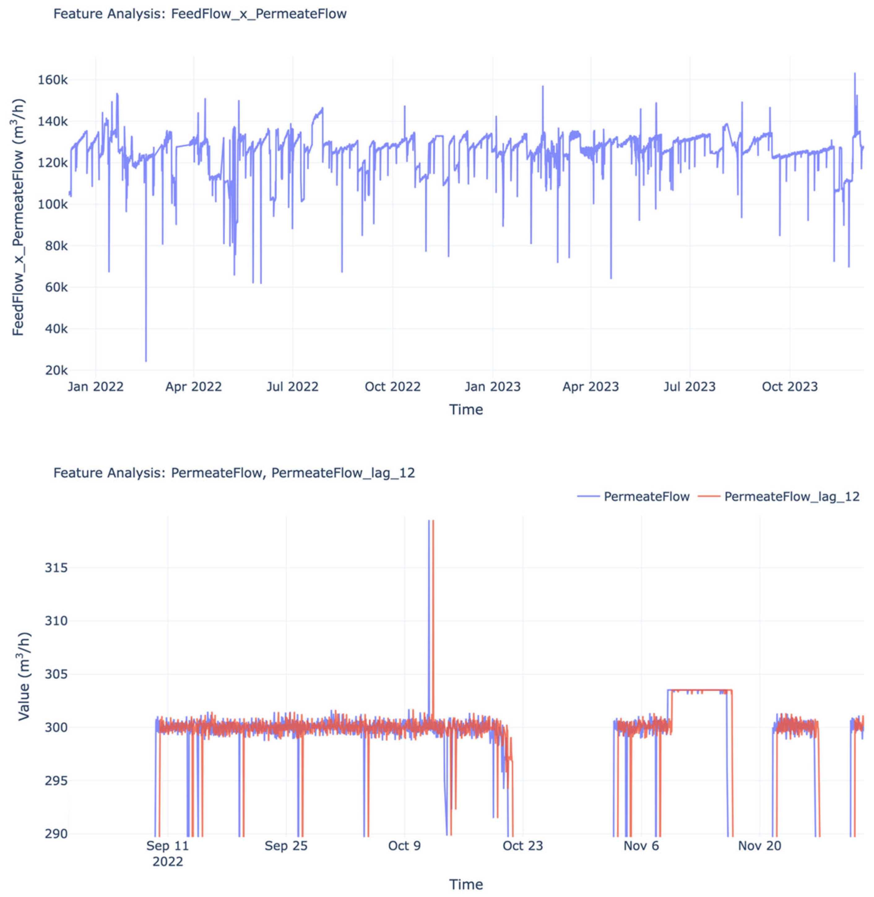
Figure 8.
Original Permeate Flow vs. Lagged Permeate Flow ( and pairwise of Feed Flow and Permeate Flow.
Figure 8.
Original Permeate Flow vs. Lagged Permeate Flow ( and pairwise of Feed Flow and Permeate Flow.
Figure 9.
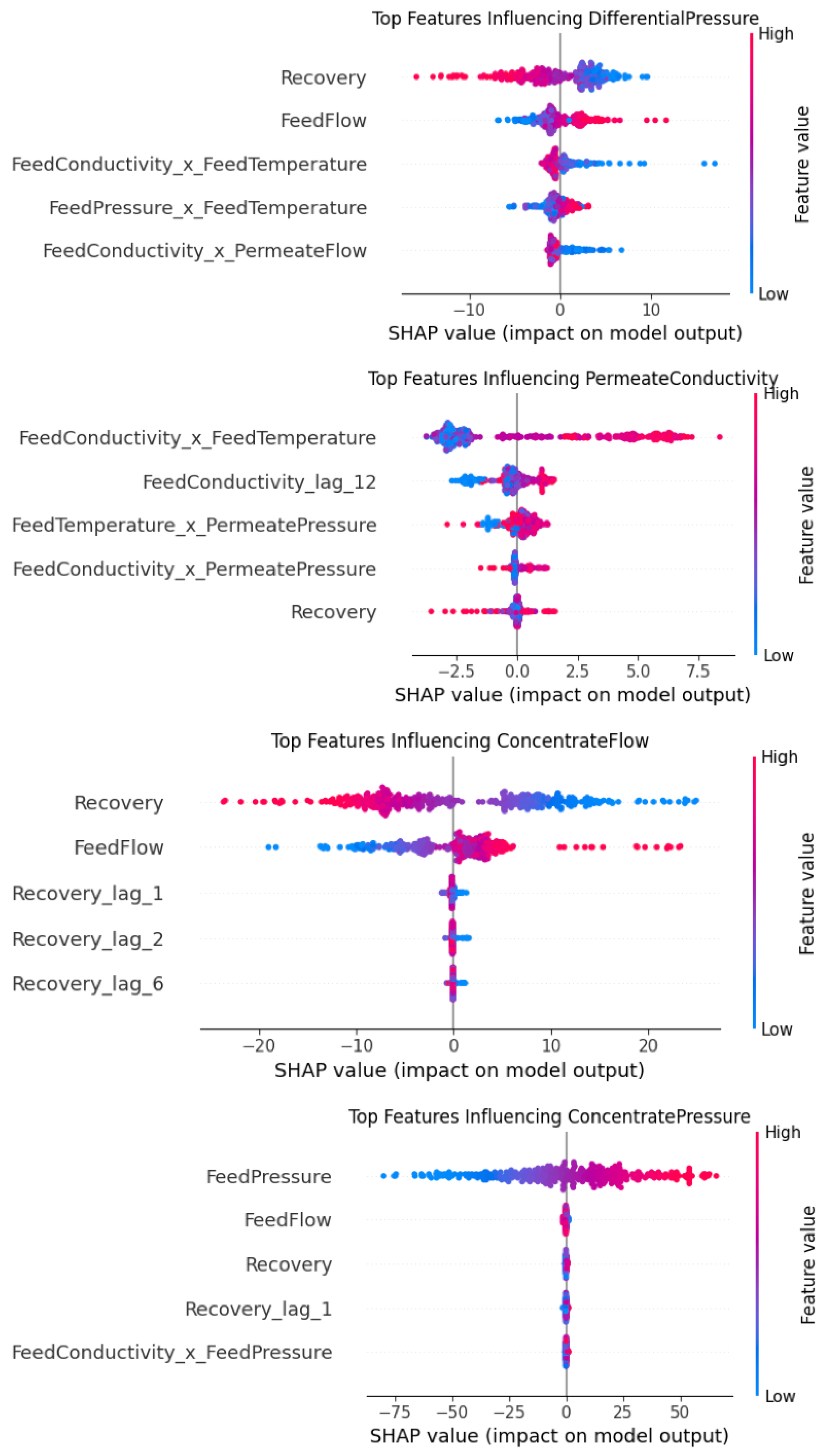
Top 5 features with SHAP analysis for all 4 target outputs.
Figure 9.
Top 5 features with SHAP analysis for all 4 target outputs.
Figure 10.
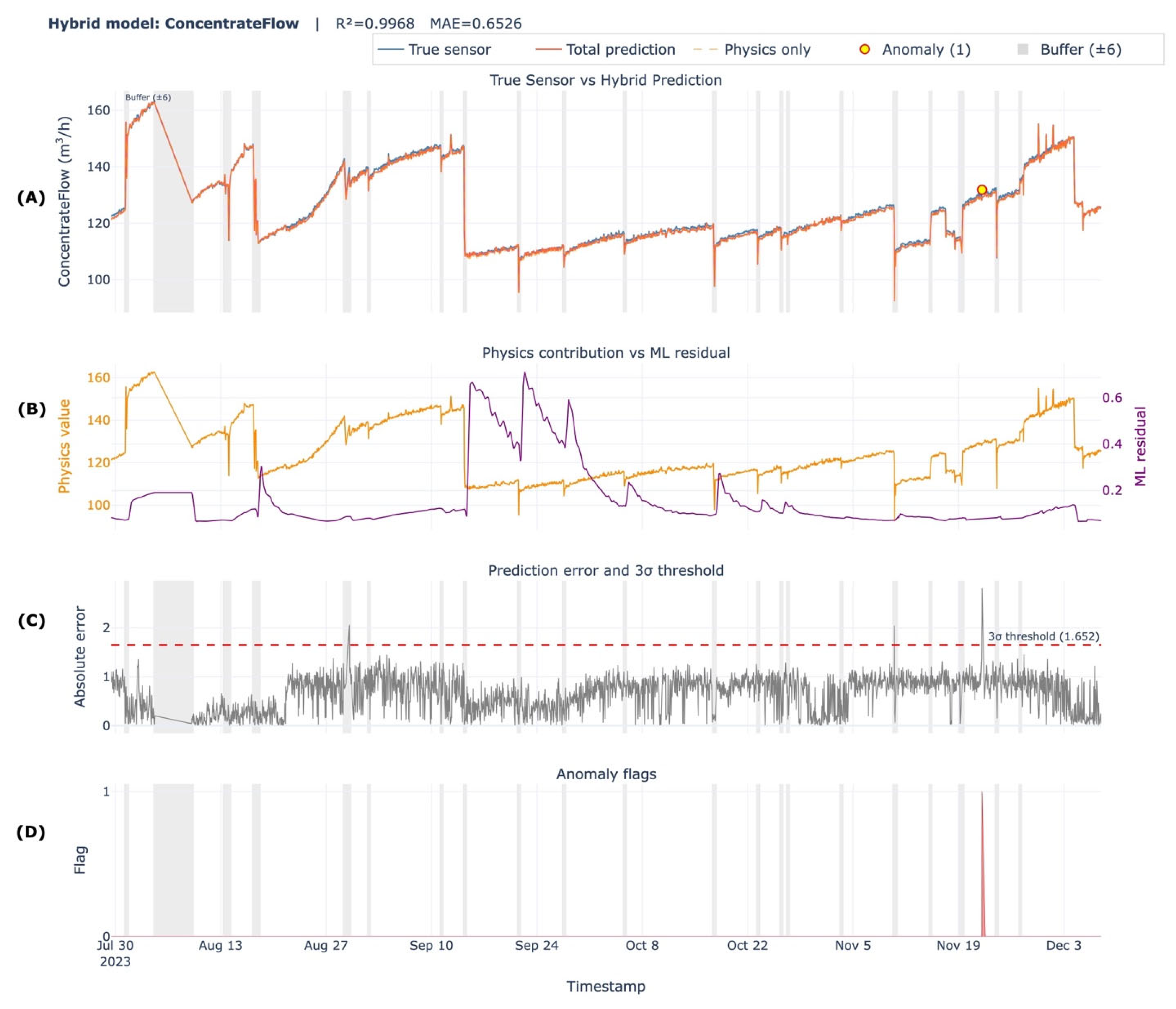
Four-panel hybrid prediction (SADS) result of Concentrate Flow, showing sensor vs. prediction (Panel (A)), physics vs. ML residual on dual axes (Panel (B)), absolute error with 3 thresholds (Panel (C)), and anomaly flag timeline with cycle buffer zones (Panel (D)).
Figure 10.
Four-panel hybrid prediction (SADS) result of Concentrate Flow, showing sensor vs. prediction (Panel (A)), physics vs. ML residual on dual axes (Panel (B)), absolute error with 3 thresholds (Panel (C)), and anomaly flag timeline with cycle buffer zones (Panel (D)).
Figure 11.
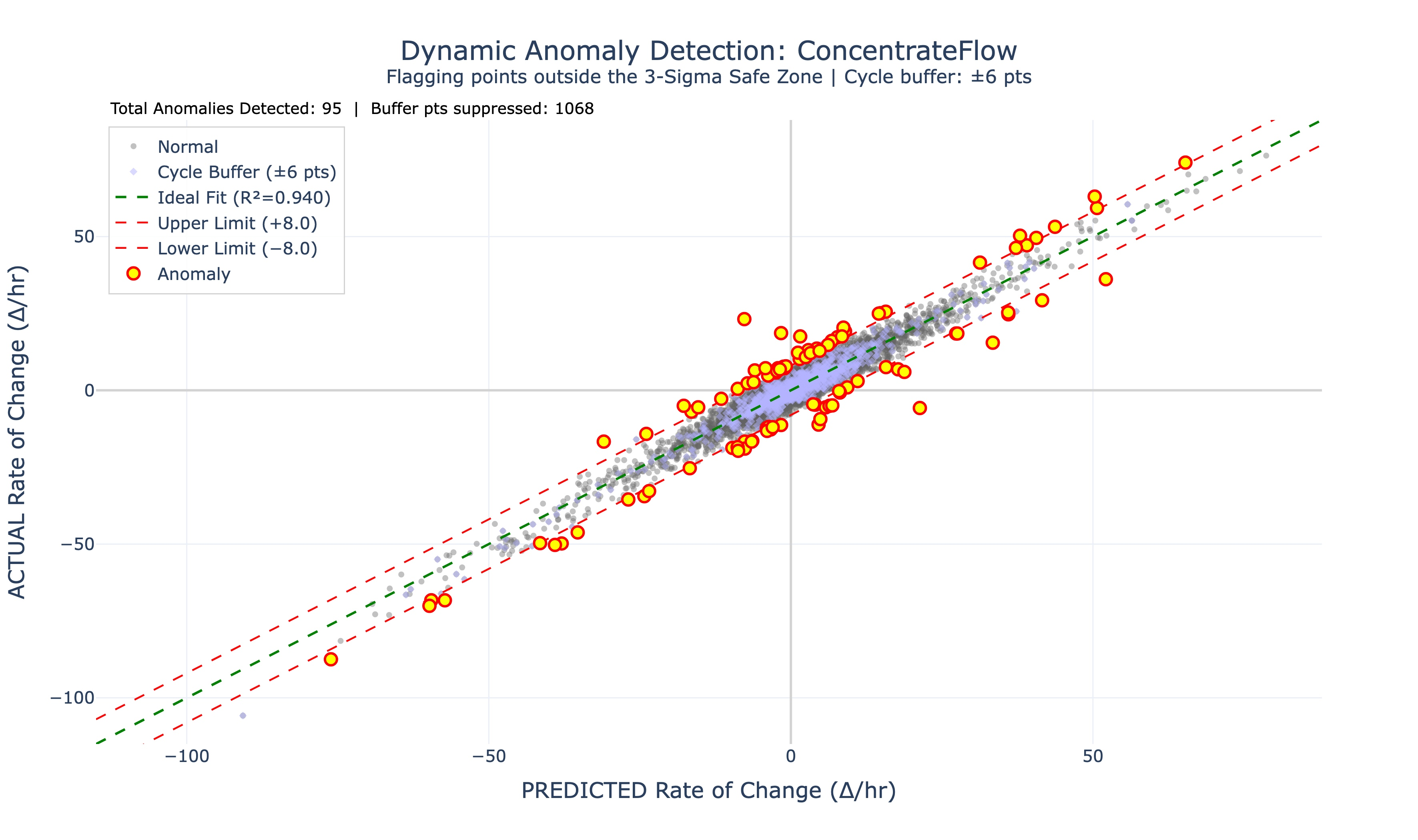
FADS results on 5 min interval data for Concentrate Flow. Grey dots are normal points; yellow dots are anomalies. All data is in first-order derivative form. The green dashed line is the ideal fit; red dashed lines are the thresholds. Data points beyond these thresholds are flagged as anomalies, except those in the cycle buffer (purple diamonds), which are excluded.
Figure 11.
FADS results on 5 min interval data for Concentrate Flow. Grey dots are normal points; yellow dots are anomalies. All data is in first-order derivative form. The green dashed line is the ideal fit; red dashed lines are the thresholds. Data points beyond these thresholds are flagged as anomalies, except those in the cycle buffer (purple diamonds), which are excluded.
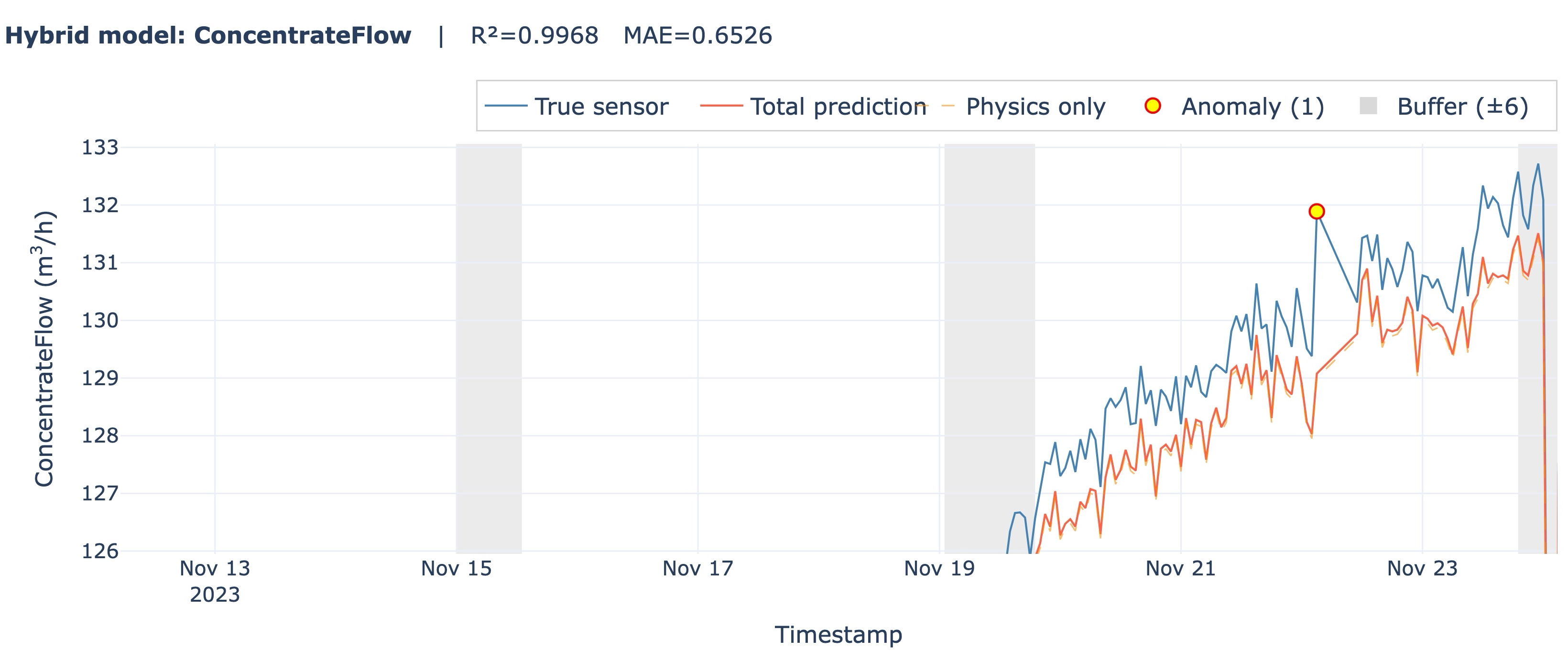
Figure 12.
The only anomaly found in Concentrate Flow.
Figure 12.
The only anomaly found in Concentrate Flow.
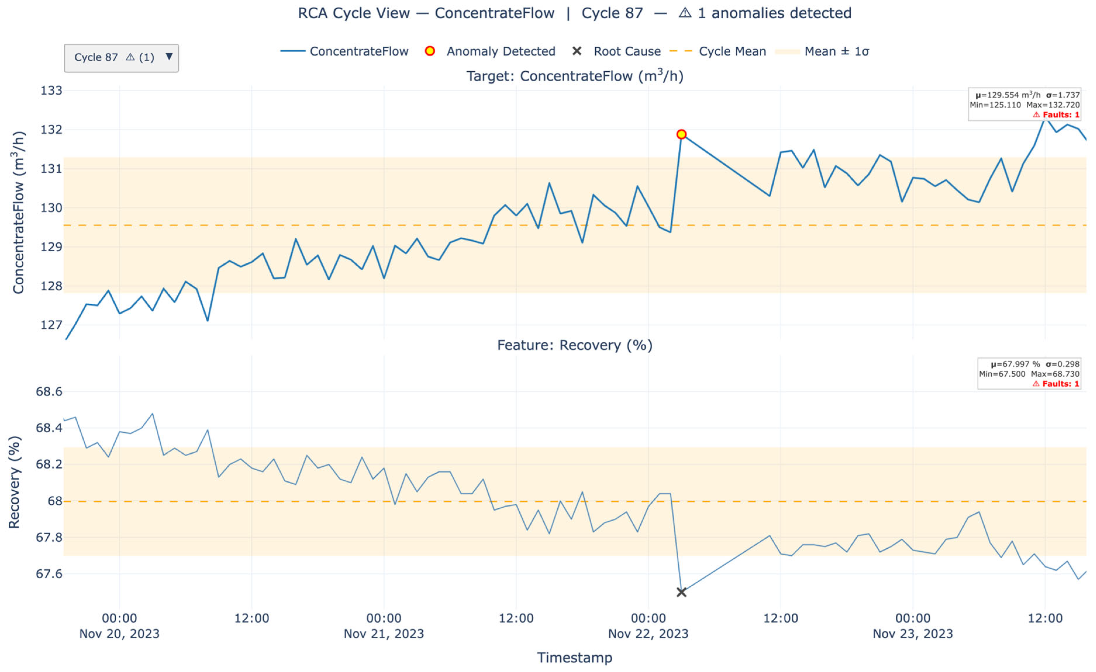
Figure 13.
RCA dashboard for Cycle 87 of Concentrate Flow.
Figure 13.
RCA dashboard for Cycle 87 of Concentrate Flow.
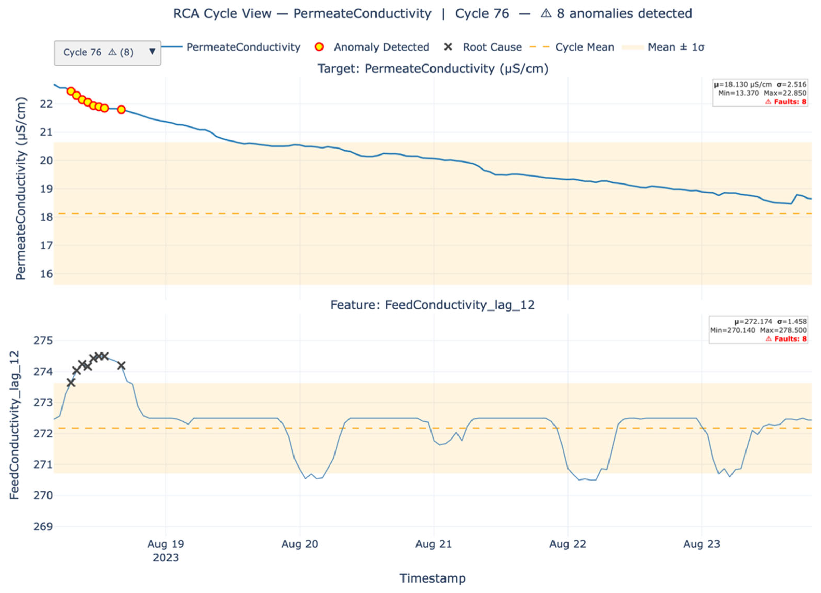
Figure 14.
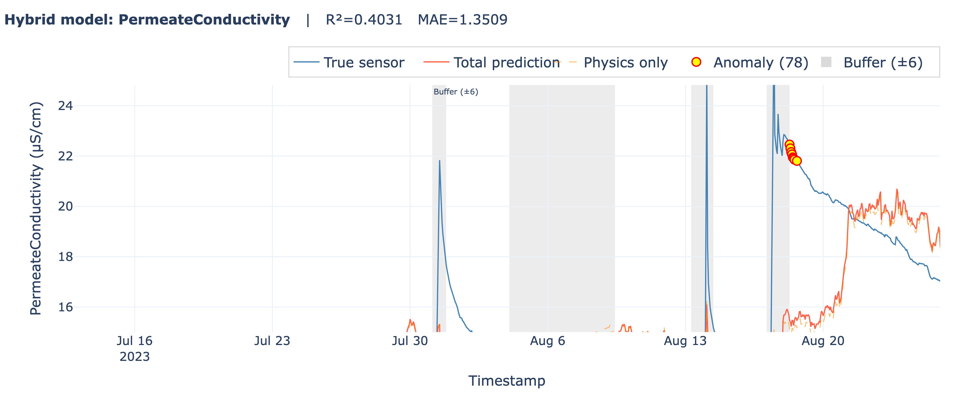
Clustered anomalies across Cycle 76 of Permeate Conductivity.
Figure 14.
Clustered anomalies across Cycle 76 of Permeate Conductivity.
Figure 15.
RCA dashboard of Cycle 76 of Permeate Conductivity.
Figure 15.
RCA dashboard of Cycle 76 of Permeate Conductivity.
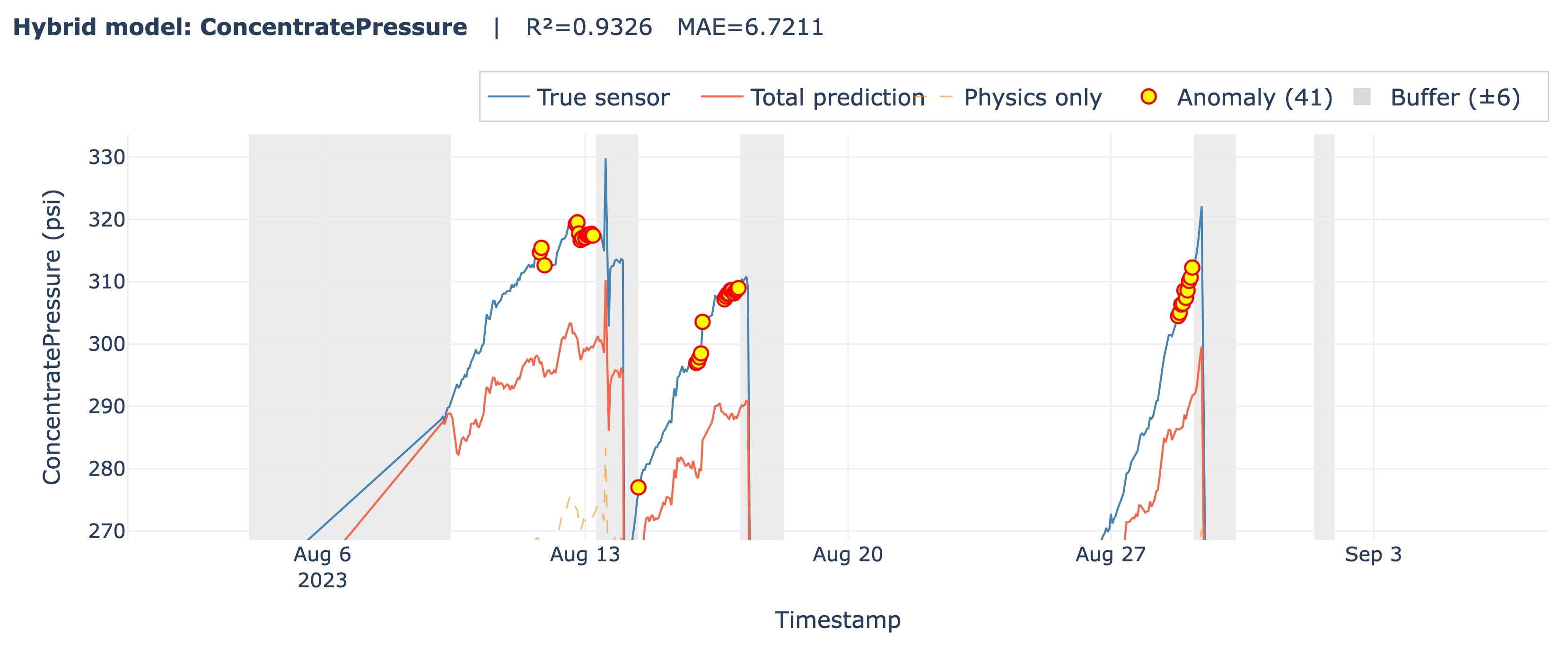
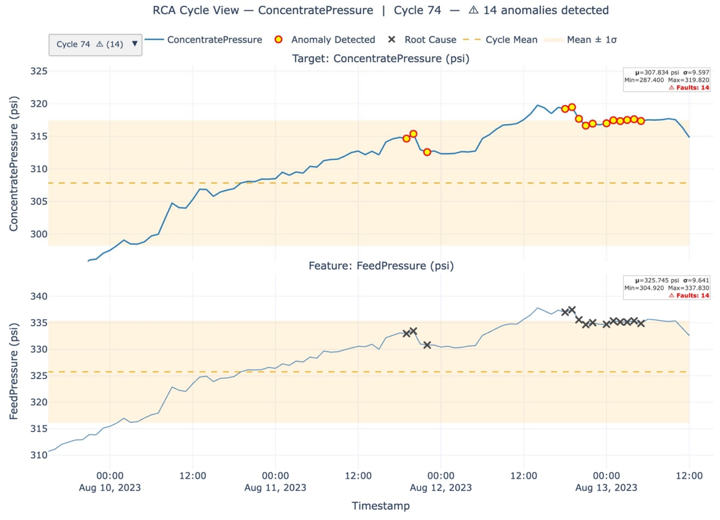
Figure 16.
Clustered anomalies across Cycle 74–76 of Concentrate Pressure.
Figure 16.
Clustered anomalies across Cycle 74–76 of Concentrate Pressure.
Figure 17.
RCA dashboard of Cycle 74 of Concentrate Pressure.
Figure 17.
RCA dashboard of Cycle 74 of Concentrate Pressure.
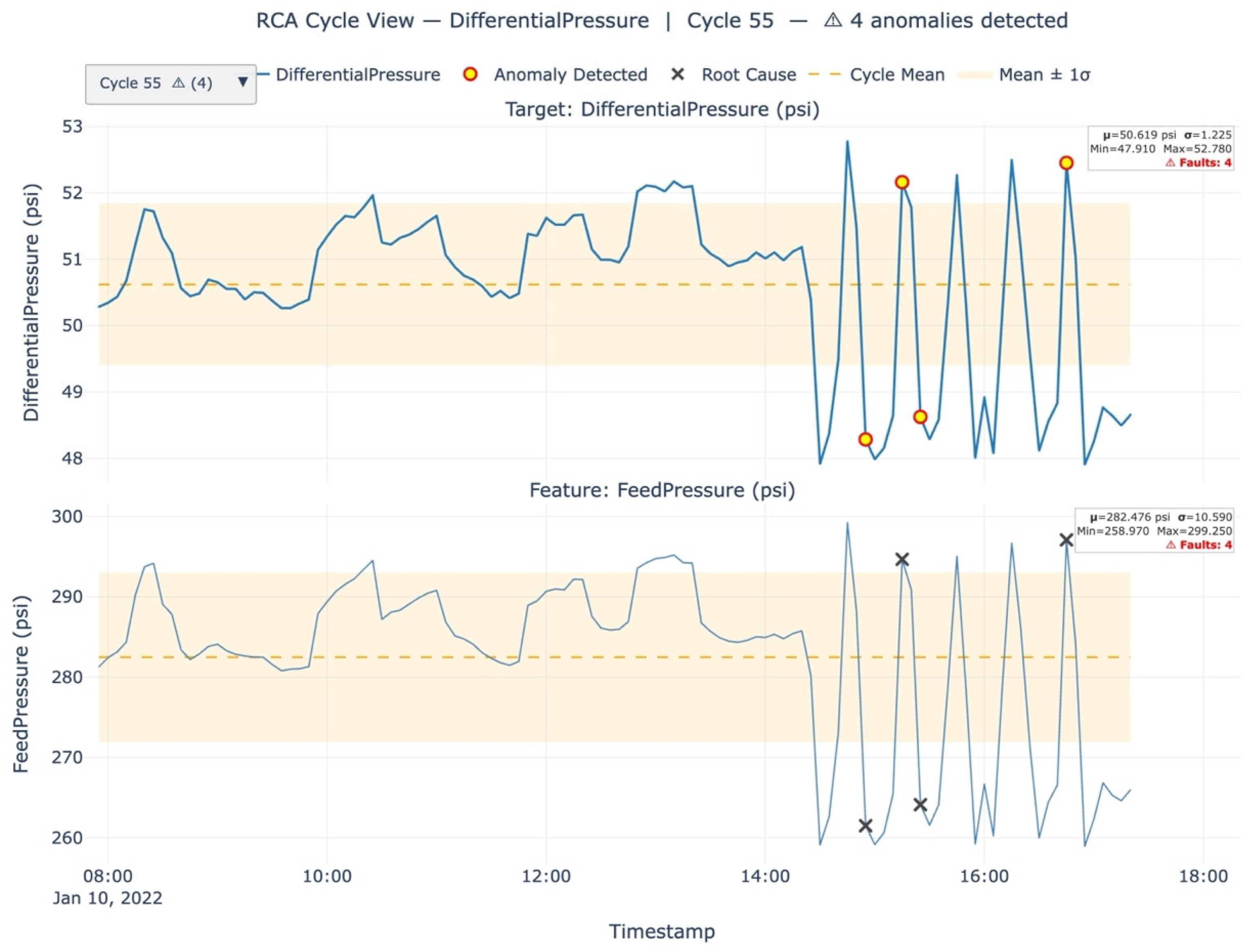
Figure 18.
RCA dashboard of Cycle 55 of Differential Pressure.
Figure 18.
RCA dashboard of Cycle 55 of Differential Pressure.
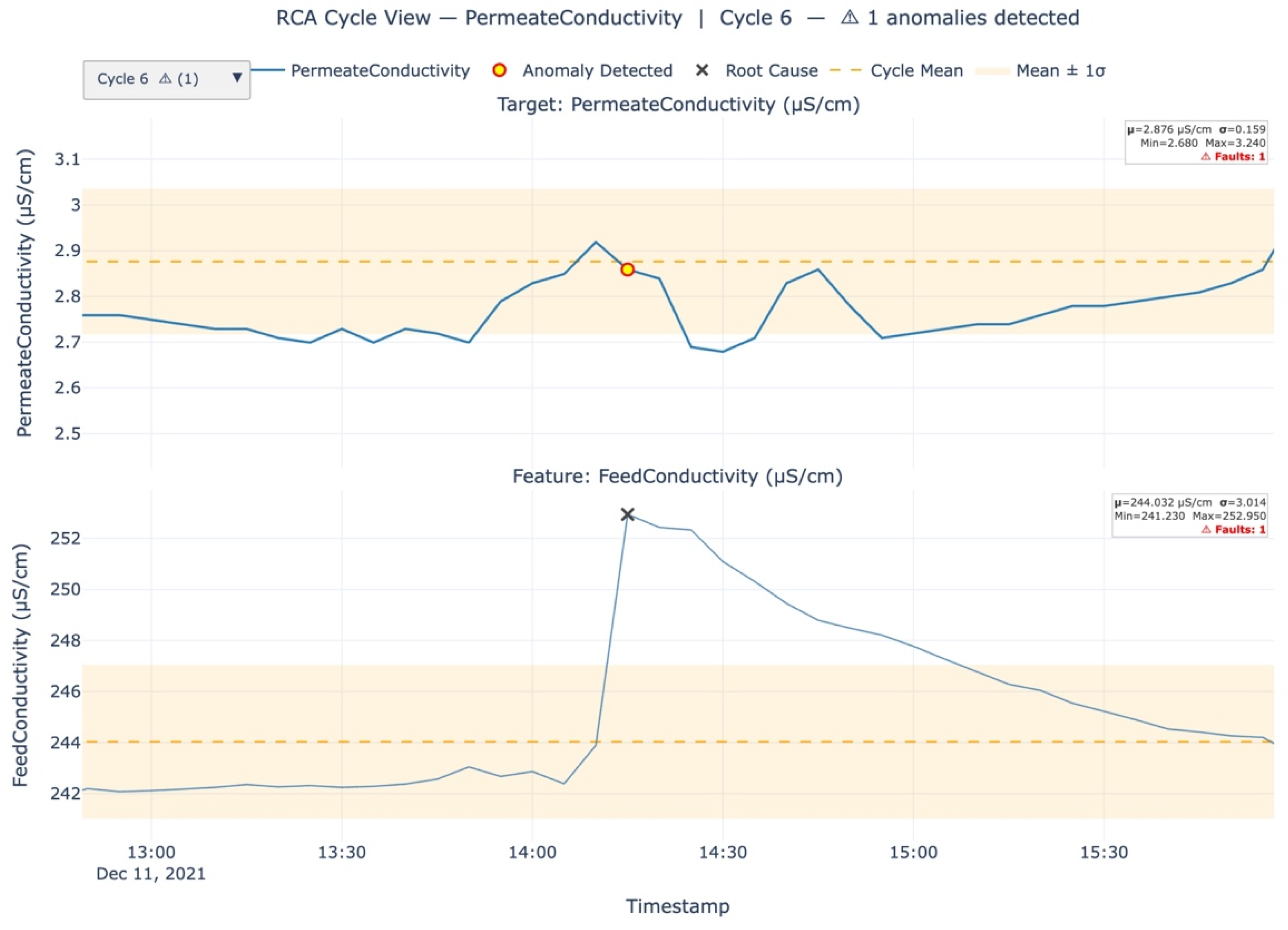
Figure 19.
RCA dashboard of Cycle 6 of Permeate Conductivity.
Figure 19.
RCA dashboard of Cycle 6 of Permeate Conductivity.
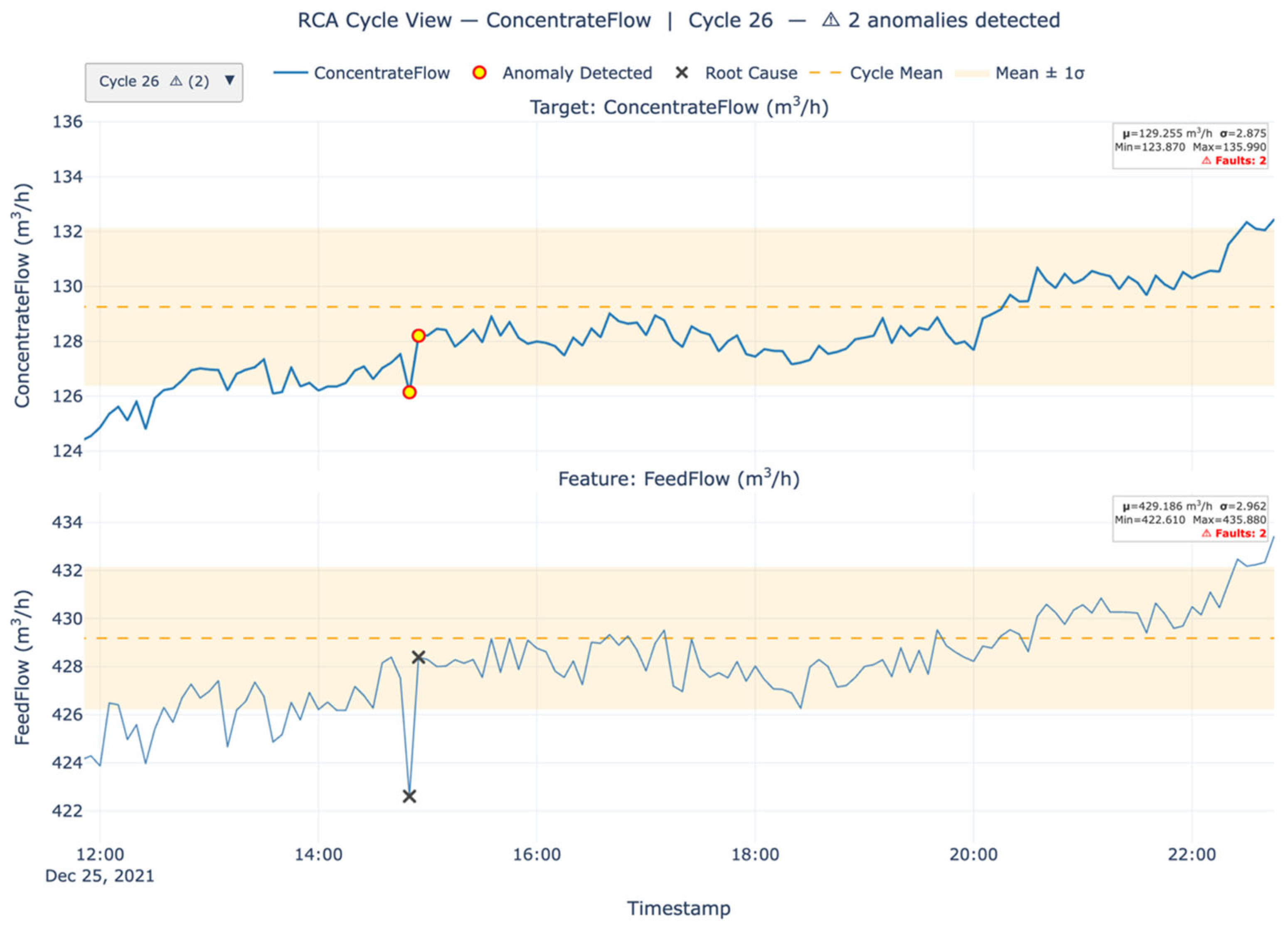
Figure 20.
RCA dashboard of Cycle 26 of Concentrate Flow.
Figure 20.
RCA dashboard of Cycle 26 of Concentrate Flow.
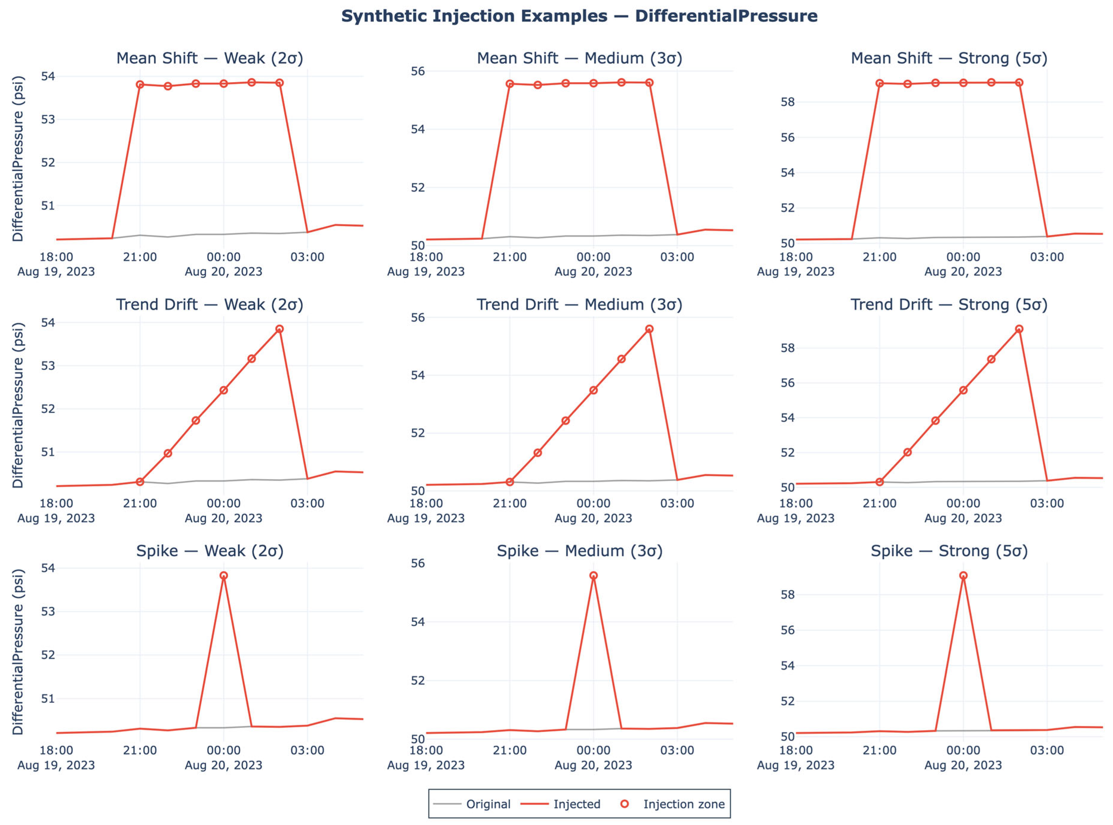
Figure 21.
An example of synthetic injected anomalies of Differential Pressure (red line and red dot) with 3 anomaly types 3 severities across 20 windows plotting alongside its original sensor absolute values (grey line) for SADS.
Figure 21.
An example of synthetic injected anomalies of Differential Pressure (red line and red dot) with 3 anomaly types 3 severities across 20 windows plotting alongside its original sensor absolute values (grey line) for SADS.
Figure 22.
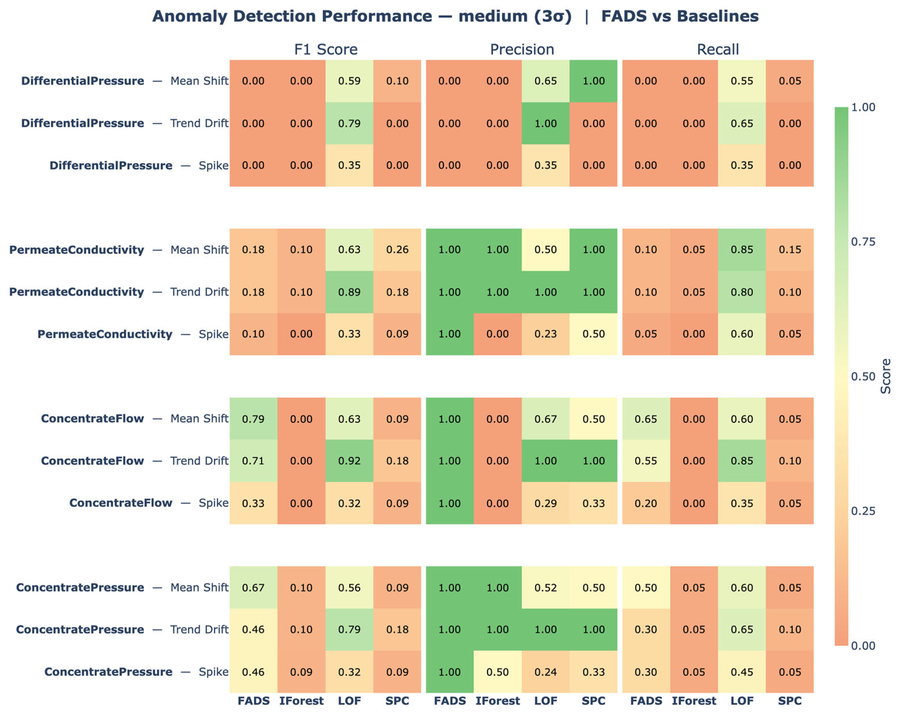
Heatmaps of F1 score, precision, and recall of FADS against three baselines for all output variables (severity ).
Figure 22.
Heatmaps of F1 score, precision, and recall of FADS against three baselines for all output variables (severity ).
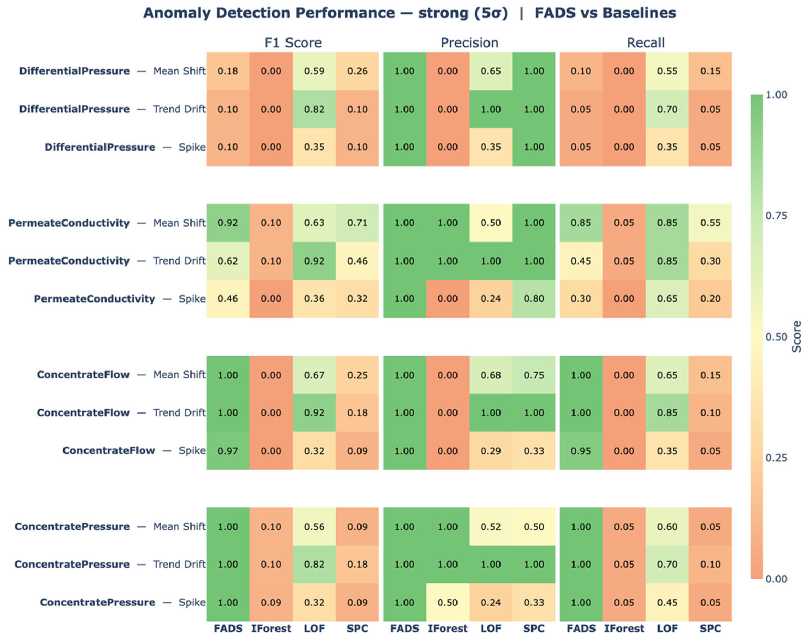
Figure 23.
Heatmaps of F1 score, precision, and recall of FADS against three baselines for all output variables (severity ).
Figure 23.
Heatmaps of F1 score, precision, and recall of FADS against three baselines for all output variables (severity ).
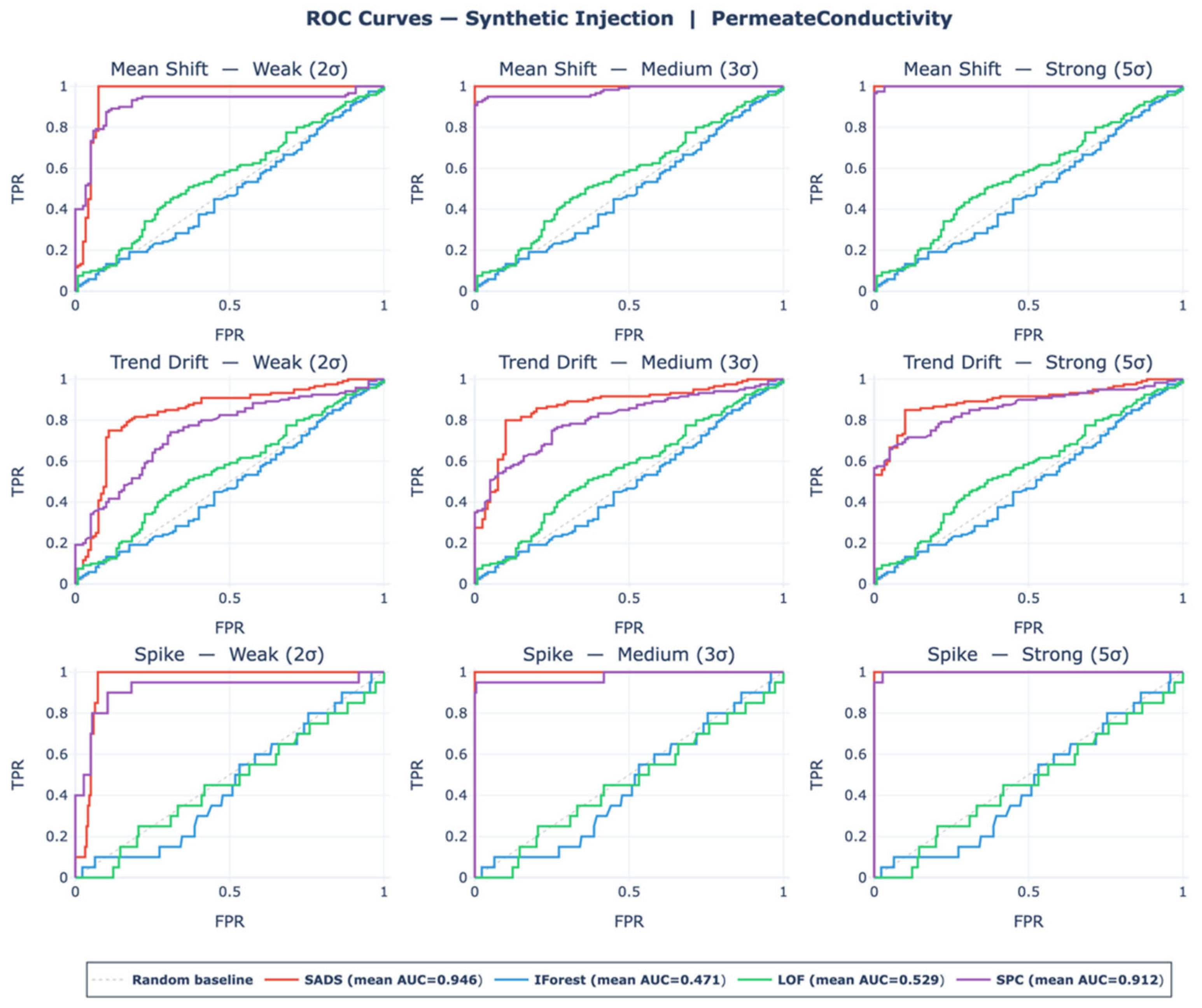
Figure 24.
ROC curves for SADS and its baselines for Permeate Conductivity.
Figure 24.
ROC curves for SADS and its baselines for Permeate Conductivity.
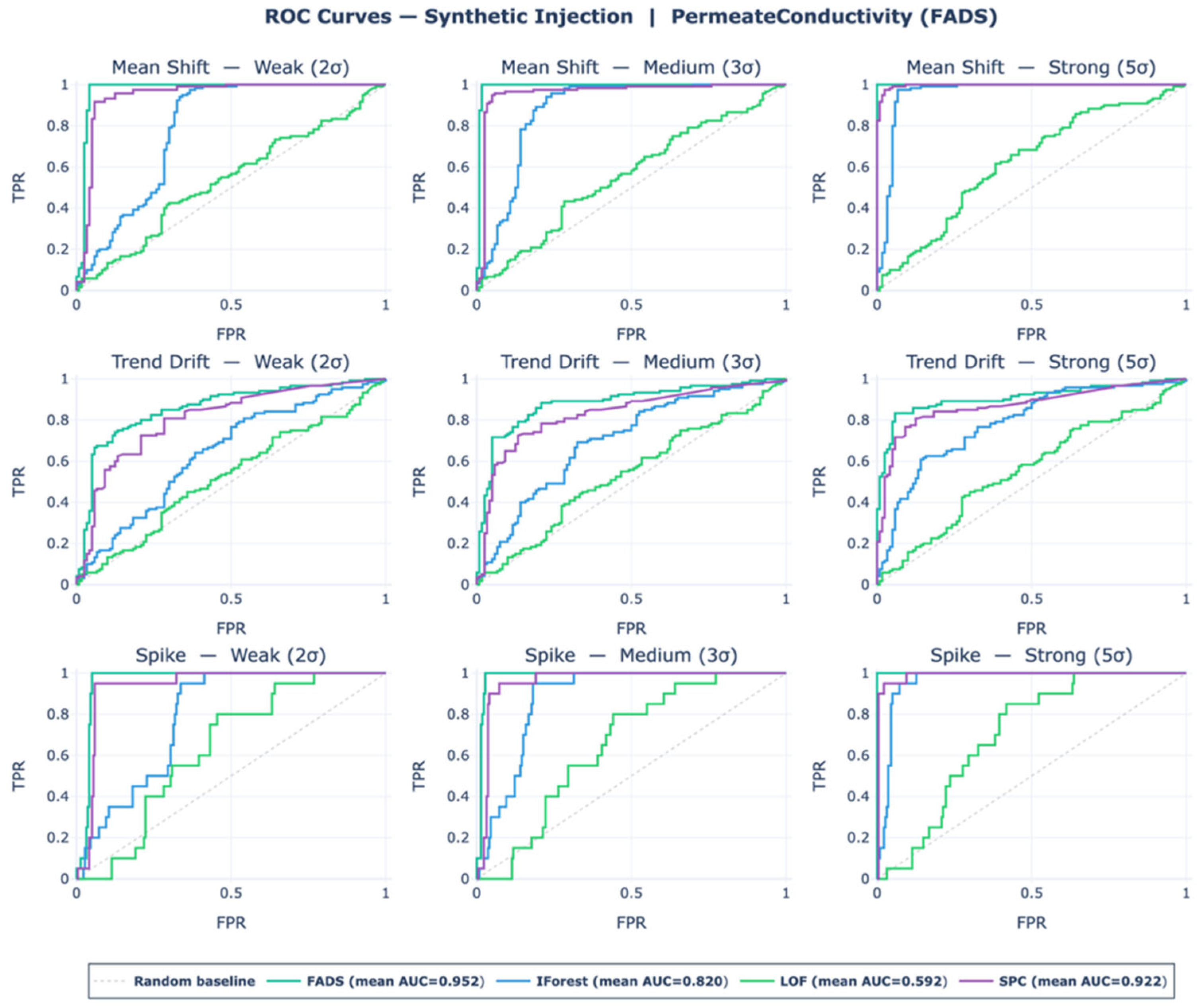
Figure 25.
ROC curves for FADS and its baselines for Permeate Conductivity.
Figure 25.
ROC curves for FADS and its baselines for Permeate Conductivity.
Table 1.
Summary of SADS and FADS.
Table 1.
Summary of SADS and FADS.
| Property | SADS | FADS |
|---|
| Operating domain | Absolute value | Rate of change (derivative) |
| Predictive model | Physics model + LSTM with attention | Multivariate linear regression |
| Justification for model choice | Nonlinear long-range temporal dependencies | Local linearity of derivatives |
| Target timescale | Slow drift, gradual degradation or slow timestamp interval | Sudden spikes, abrupt faults or fast timestamp interval |
| Computational cost | Relatively high | Low |
| Real-time suitability | No | Yes |
| Anomaly score | | |
| Detection threshold | | |
Table 2.
Data characteristics.
Table 2.
Data characteristics.
| Property | Description |
|---|
| Source | SCADA system, RO water treatment plant, China |
| Duration | 2 years |
| Sampling intervals | 1 h (SADS dataset); 5 min (FADS dataset), independently recorded |
| Number of variables | 11 (process variable) + 1 (timestamp) |
Table 3.
List of process variables used in this paper.
Table 3.
List of process variables used in this paper.
| Variable Name | Unit | Type | Justification |
|---|
| Concentrate Flow | gpm | Output | Resultant from mass balance |
| Concentrate Pressure | psi | Output | Resultant from pressure balance |
| Feed Flow | gpm | Input | Flow of source water entering the RO system |
| Feed Pressure | psi | Input | Hydraulic pressure in the feed side of the RO membrane |
| Feed Conductivity | µS/cm | Input | Reflects source water quality; not controlled by the RO system itself |
| Feed Temperature | °F | Input | Ambient-dependent variable that affects membrane permeability |
| Differential Pressure | psi | Output | Fouling state indicator |
| Permeate Flow | gpm | Input | Operationally setpoint; controller compensation statistically entangled with fouling |
| Permeate Pressure | psi | Input | Operationally setpoint |
| Permeate Conductivity | μS/cm | Output | Conductivity of purified permeate stream |
| Recovery | % | Input | Ratio of permeate flow to feed flow |
Table 4.
Hyperparameters used in this application.
Table 4.
Hyperparameters used in this application.
| Hyperparameters | Value |
|---|
| Hidden dimension | 64 units |
| Number of LSTM layers | 1 |
| Sequence length | 12-time steps (12 h) |
| Dropout | 0.2 |
| Optimizer | AdamW ( ) |
| Loss function | Huber loss |
| Batch size | 64 |
| Seed | 42 |
| Train/validation split | 80%/20% |
| Train/test split | 80%/20% |
Table 5.
SADS hybrid model performance on the test set (2988 timestamps).
Table 5.
SADS hybrid model performance on the test set (2988 timestamps).
| Output | Hybrid | MAE | Threshold | Anomalies |
|---|
| Differential Pressure | 0.543 | 2.48 | 9.36 | 0 |
| Permeate Conductivity | 0.403 | 1.35 | 6.28 | 78 |
| Concentrate Pressure | 0.932 | 6.72 | 17.7 | 41 |
| Concentrate Flow | 0.997 | 0.65 | 1.65 | 1 |
Table 6.
List of input features used in model training for FADS.
Table 6.
List of input features used in model training for FADS.
| Target Output | Input Features (After Extracted from Top 5 Features by SHAP) |
|---|
| Differential Pressure | Feed Pressure, Permeate Flow, Feed Flow, Feed Conductivity, Feed Temperature, Recovery |
| Permeate Conductivity | Feed Conductivity, Permeate Pressure, Feed Temperature |
| Concentrate Flow | Recovery, Feed Flow |
| Concentrate Pressure | Feed Pressure, Feed Flow, Recovery, Feed Conductivity |
Table 7.
Summary of FADS results for each output.
Table 7.
Summary of FADS results for each output.
| Output Variable | Anomalies Detected | |
|---|
| Differential Pressure | 75 | 0.650 |
| Permeate Conductivity | 154 | 0.234 |
| Concentrate Flow | 95 | 0.940 |
| Concentrate Pressure | 125 | 0.993 |
Table 8.
Component ablation (Differential Pressure).
Table 8.
Component ablation (Differential Pressure).
| Variant | R2 | MAE | F1 @ | F1 @ | F1 @ |
|---|
| Physics only | −1.12 | 8.612 | 0.113 | 0.297 | 0.792 |
| Standalone LSTM (no physics) | 0.104 | 3.738 | 0.160 | 0.219 | 0.725 |
| Hybrid (full model) | 0.543 | 2.478 | 0.088 | 0.227 | 0.750 |
| Hybrid, no attention | 0.542 | 2.649 | 0.000 | 0.000 | 0.500 |
| Hybrid, no cyclic features | (identical to full model not used) | | | | |
Table 9.
SADS vs. FADS detection F1 (Differential Pressure).
Table 9.
SADS vs. FADS detection F1 (Differential Pressure).
| Anomaly Type | SADS F1 (Avg.) | FADS F1 (Avg.) |
|---|
| Mean shift | 0.467 | 0.061 |
| Spike | 0.434 | 0.032 |
| Trend drift | 0.434 | 0.000 |
Table 10.
Top 1/Top 3 accuracy results for RCA module validation.
Table 10.
Top 1/Top 3 accuracy results for RCA module validation.
| Target | Top 1 Accuracy | Top 3 Accuracy | Dominant Sensor (β) |
|---|
| Differential Pressure | 0.290 | 0.947 | Recovery (0.890) |
| Permeate Conductivity | 0.400 | 0.776 | Recovery (0.614) |
| Concentrate Flow | 0.607 | 0.889 | Recovery (0.666) |
| Concentrate Pressure | 0.359 | 0.703 | Feed Pressure (0.869) |
Table 11.
SADS-vs.-FADS chance-normalized comparison.
Table 11.
SADS-vs.-FADS chance-normalized comparison.
| System | Target | Candidates | Top 1 Accuracy | Top 1/Chance | Dominant Driver (Share) |
|---|
| SADS | Differential Pressure | 5 | 0.290 | 1.45× | Recovery (0.89) |
| SADS | Permeate Conductivity | 5 | 0.400 | 2.00× | Recovery (0.61) |
| SADS | Concentrate Flow | 5 | 0.607 | 3.04× | Recovery (0.67) |
| SADS | Concentrate Pressure | 5 | 0.359 | 1.80× | Feed Pressure (0.87) |
| FADS | Differential Pressure | 6 | 0.567 | 3.40× | Recovery (0.64) |
| FADS | Permeate Conductivity | 3 | 0.679 | 2.04× | Feed Temperature (0.65) |
| FADS | Concentrate Pressure | 4 | 0.256 | 1.02× | Feed Pressure (0.92) |
| FADS | Concentrate Flow | 2 | 0.845 | 1.69× | Recovery (0.93) |
Table 12.
F1 by severity, fixed vs. 99th-percentile quantile threshold.
Table 12.
F1 by severity, fixed vs. 99th-percentile quantile threshold.
| System | Target | Method | Weak () | Moderate () | Strong () |
|---|
| SADS | Differential Pressure | /Quantile | 0.067/0.188 | 0.175/0.493 | 0.759/0.850 |
| SADS | Concentrate Flow | /Quantile | 0.237/0.606 | 0.583/0.785 | 0.852/0.894 |
| SADS | Concentrate Pressure | /Quantile | 0.074/0.074 | 0.175/0.175 | 0.805/0.805 |
| SADS | Permeate Conductivity | /Quantile | 0.081/0.060 | 0.136/0.129 | 0.815/0.794 |
| FADS | Differential Pressure | /Quantile | 0.000/0.000 | 0.000/0.000 | 0.015/0.000 |
| FADS | Permeate Conductivity | /Quantile | 0.023/0.000 | 0.060/0.000 | 0.278/0.052 |
| FADS | Concentrate Pressure | /Quantile | 0.160/0.116 | 0.349/0.261 | 0.827/0.815 |
| FADS | Concentrate Flow | /Quantile | 0.205/0.188 | 0.341/0.301 | 0.823/0.810 |
Table 13.
Summary of challenges identified and framework response.
Table 13.
Summary of challenges identified and framework response.
| Challenges Identified in Section 1 | Framework Response |
|---|
| Lack of fusion model integrating process physics with time-series data | Hybrid SADS combines domain-specific physics equations with an LSTM residual model calibrated on normal operating data; the physics component provides an interpretable, first-principle baseline, while the LSTM corrects the structured residual |
| Insufficient interpretability of detected anomalies | Domain-consistent RCA attributes each anomaly to its most probable input feature with direction (HIGH/LOW or rate up/down) |
| Limited generalization | Adaptation effort is tiered by pipeline step (Section 5.2): reconfiguration-only steps require hours; retraining on target-process data requires additional data collection and compute time; physics equation rederivation is the dominant cost, estimated at days to weeks depending on the maturity of existing process physics literature |
| Multi-timescale anomalies | Dual pipeline: SADS for slow drift on hourly data; FADS for abrupt deviations on 5 min data; combined flag from either system |
| Data label scarcity | Fully unsupervised: threshold requires only normal operating data; no anomaly labels required at any stage |
| Absence of cyclic analysis | Cycle-aware sequence construction prevents cross-cycle contamination; cycle buffer (6 timesteps) suppresses false positives at transitions |