Intelligent Inversion Method of Fracturing Fracture Morphology Based on G-Function Constraints and CNN-LSTM

Abstract

Addressing the challenges in quantitative characterization of post-fracture fracture geometry in unconventional reservoirs such as tight gas and shale, for which existing prediction methods provide only limited accuracy, this study proposes an intelligent inversion method for fracture morphology by integrating G-function post-fracture diagnosis with a CNN-LSTM network. The number of branch fractures determined from G-function analysis of pressure decline curves is employed as a hard constraint. Latin hypercube sampling (LHS) is adopted to generate multi-dimensional fracture geometry samples, and a CNN-LSTM model is constructed to establish the nonlinear mapping from fracture morphology to production response, thereby forming a sample database that correlates production with fracture geometry. Leveraging this database, intelligent inversion of post-fracture fracture geometry can be efficiently realized. Field validation demonstrates that the inverted fracture half-length deviates by less than 3% from microseismic monitoring results, while the production prediction error remains below 6%, significantly outperforming the 10% tolerance threshold commonly accepted in field engineering. The proposed method requires only single-well pressure decline curves and production data to accomplish post-fracture fracture geometry evaluation, exhibiting broad application prospects.

1. Introduction

Unconventional oil and gas resources such as tight gas and shale gas have become an important component of the global energy structure [1]. Due to the generally low porosity and low permeability of such reservoirs, hydraulic fracturing is a key technology for achieving economic production [2]. The morphology of the fracture network formed by hydraulic fracturing directly determines hydrocarbon flow paths and production efficiency; accurate knowledge of fracture geometric parameters is therefore indispensable for evaluating fracturing schemes, predicting remaining gas distribution, and formulating subsequent development strategies [3]. However, post-fracture fracture morphology is buried thousands of meters underground, making direct observation extremely difficult. How to economically, efficiently, and accurately quantitatively characterize fracture morphology has thus remained one of the core challenges in petroleum engineering [4,5].

Current methods for post-fracture fracture morphology diagnosis mainly fall into three categories: pressure analysis, monitoring techniques, and numerical simulation. Among these, the G-function theory proposed by Nolte is the most widely applied pressure analysis method [6]. Subsequently refined by Barree, Craig [7], it has become an important tool for identifying fracture closure characteristics and communication with natural fractures. By analyzing the first derivative dP/dG and the superposition derivative G·dP/dG of pressure decline curves, one can determine whether fractures communicate with natural fractures and estimate parameters such as fracture half-length and closure pressure. However, conventional G-function methods can only obtain limited fracture parameter information, failing to fully construct fracture morphology models that encompass multi-dimensional geometric features. Moreover, diagnostic results are highly sensitive to factors such as pressure data quality and leakoff model assumptions.

In terms of monitoring techniques, microseismic monitoring, which infers the spatial distribution of fractures by capturing microseismic events induced by hydraulic fracturing, is currently the most widely applied real-time fracture monitoring technology. Nevertheless, microseismic monitoring suffers from inherent limitations such as a high detection threshold, event location accuracy strongly affected by velocity models, and highly non-unique interpretation results [8]. Furthermore, the quantitative mapping relationship between microseismic events and fracture geometric parameters remains ambiguous; fracture complexity, reservoir heterogeneity, and operational parameters collectively constrain the reliability of monitoring interpretation [9]. Emerging technologies such as tracer testing and distributed fiber-optic sensing (DAS/DTS) can provide fracture connectivity information, yet they are costly and operationally complex, and likewise fail to quantitatively deliver key geometric parameters such as fracture length, width, and conductivity. Although inversion methods based on reservoir numerical simulation can theoretically yield complete fracture geometries, they are computationally intensive, with a single inversion often requiring tens of minutes to several hours, and are sensitive to initial model assumptions, making it difficult to satisfy the demand for rapid decision-making in field operations.

In recent years, artificial intelligence (AI) technologies, particularly deep learning methods, have demonstrated substantial application potential in petroleum engineering, and intelligent hydraulic fracturing has been recognized as an important development direction of the industry. In the domain of fracture identification and characterization, convolutional neural networks (CNNs) have been successfully applied to tasks such as automatic classification of microseismic events, fracture identification from well logs, and fracturing parameter optimization; LSTM-based surrogate models have also been developed to replace full-physics fracture propagation simulators, substantially reducing the computational cost of forward modeling. In the domain of production forecasting, long short-term memory (LSTM) networks and their variants exhibit excellent performance in time-series modeling: Pan et al. [10] combined a CNN-LSTM network with a self-attention mechanism for oil well production prediction; Zhou et al. [11] embedded an empirical decline model as a physical constraint into a CNN-LSTM framework for shale oil production prediction; and improved architectures, including CNN-BiLSTM with attention mechanisms [12] and CNN-LSTM networks optimized by intelligent search algorithms [13], have been reported successively, together with machine learning-based shale gas production prediction and optimization studies [14]. CNN-LSTM hybrid models combine the spatial feature extraction capability of CNNs with the temporal dynamic learning ability of LSTM networks, demonstrating significant advantages in multivariate prediction for complex systems.

Despite these advances, a clear scientific gap remains. First, existing AI studies in this field predominantly employ purely data-driven end-to-end modeling strategies that directly map fracturing operational or geological parameters to production or fracture morphology, without explicit physical constraints; the resulting models may generate physically implausible solutions and exhibit limited interpretability [14]. Second, although surrogate (proxy) models substantially accelerate forward simulation, proxy-based history matching still requires case-by-case iterative optimization to invert fracture parameters, and the diagnostic information contained in post-fracture pressure decline data, which is routinely acquired at negligible cost, is seldom exploited in the inversion loop. Third, the G-function diagnosis can provide the branch fracture count as independent physical evidence of fracture complexity, yet no existing study has incorporated such diagnostic results as a hard constraint into a deep-learning inversion framework. Bridging this gap, namely integrating pressure decline diagnostics with deep-learning inversion, constitutes the motivation of this study.

In view of this, an intelligent inversion method for fracturing fracture morphology based on G-function constraints and CNN-LSTM is proposed in this study. The number of branch fractures obtained from G-function post-fracture diagnosis is incorporated as a hard constraint into the inversion workflow, which effectively prevents physically implausible solutions that may arise in purely data-driven models and enhances both the interpretability and reliability of the model. A hybrid CNN-LSTM neural network architecture is constructed, fully leveraging the advantage of convolutional layers in extracting high-order coupling features among fracture parameters and the strength of LSTM layers in learning temporal dynamic patterns of production, thereby achieving a high-precision nonlinear mapping from fracture morphology to production response. Compared with existing proxy-based history matching methods, the proposed approach offers three advantages: (i) the G-function diagnosis physically confines the inversion to the candidate subspace consistent with the actual fracture complexity, instead of searching the entire parameter space blindly; (ii) the inversion is accomplished by matching against a pre-generated fracture–production database, avoiding the case-by-case iterative forward simulation required by surrogate-based history matching, so that a single inversion is completed within minutes using only single-well pressure decline and production data; and (iii) the physical constraint endows the model with an interpretability that purely statistical proxies lack. By integrating G-function physical diagnosis with deep learning inversion, this method provides a technical pathway for quantitative characterization of fracturing fracture morphology that simultaneously possesses interpretability and computational efficiency.

2. Fracture Morphology Inversion Model Based on G-Function Constraints

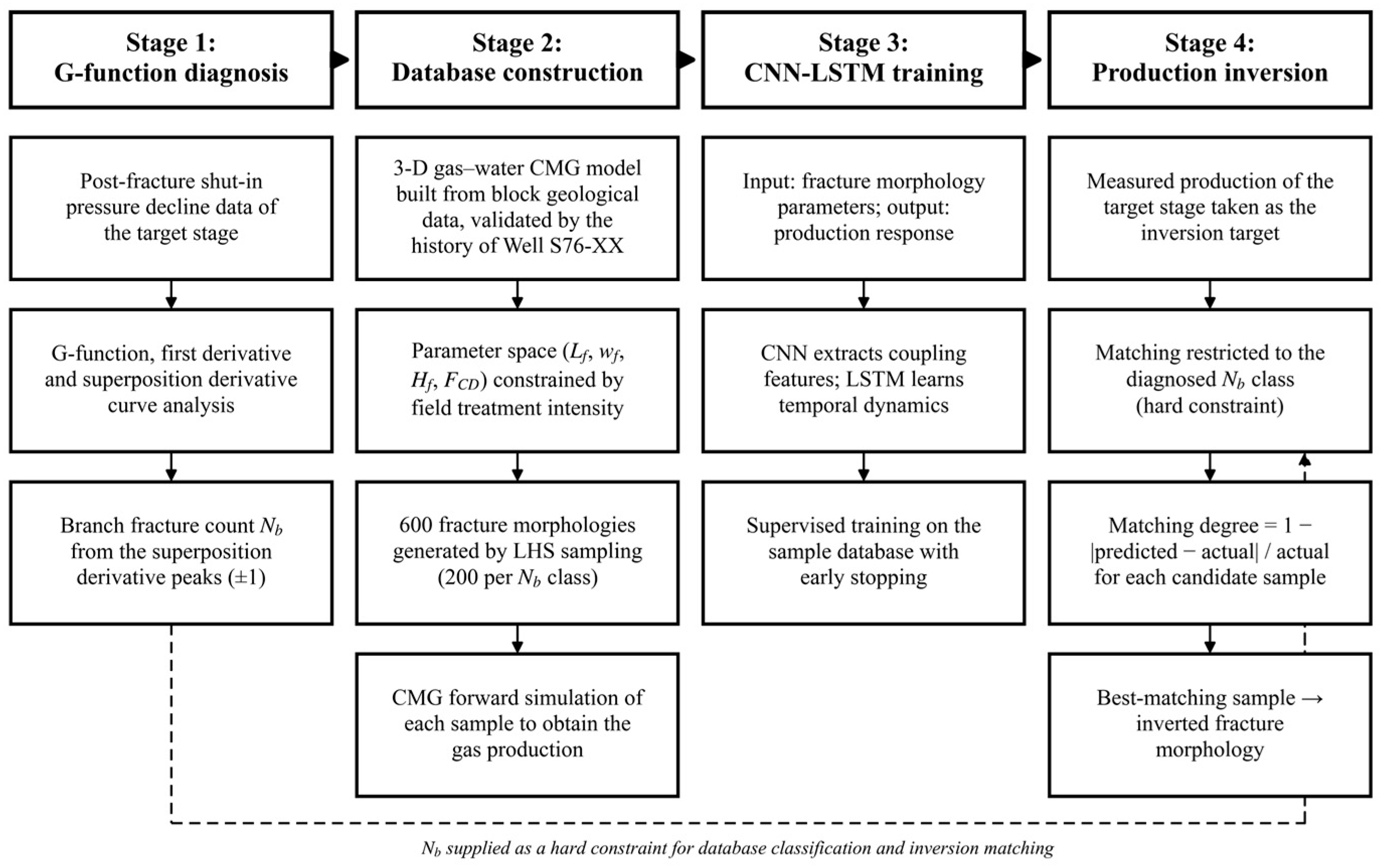
The overall workflow of the proposed method is illustrated in Figure 1. The branch fracture count of the target stage is first diagnosed from the post-fracture pressure decline data through G-function analysis and is imposed as a hard constraint throughout the subsequent inversion. A fracture–production mapping database is then constructed through CMG forward simulations of Latin hypercube-sampled fracture morphologies, on which the CNN-LSTM network is trained. Finally, the fracture morphology of the target stage is inverted by matching the measured production within the diagnosed complexity class.

2.1. G-Function Post-Fracture Diagnosis and Determination of Branch Fracture Count

The G-function analysis proposed by Nolte in 1979 is a classical method for post-fracture fracture diagnosis. Subsequently improved and refined by Castillo [15], Barree [7], and other scholars, it has become an important tool for identifying fracture closure characteristics and communication with natural fractures. The G-function is established based on fracturing fluid leakoff theory. By constructing a dimensionless time function, it standardizes pressure decline curves, thereby eliminating the effects of pumping time and leakoff characteristics and rendering pressure decline data from different well sections and operational scales comparable.

The classical G-function expression describes the relationship among leakoff area, leakoff coefficient, and dimensionless time. Let the dimensionless time θ = t/t_p, where t_p is the pumping time; the G-function can then be expressed as

$$G({\alpha }_c,{\alpha }_s,\theta )={\displaystyle {\int }_1^{\theta }{\xi }^{{\alpha }_s+{\alpha }_c-\frac{1}{2}}}{\displaystyle {\int }_0^{\xi -{\alpha }_c}\frac{d\lambda }{\sqrt{1-{\lambda }^{\frac{4}{{\alpha }_c}}}}}d\xi$$

(1)

where α_s is the parameter characterizing the time-dependent variation of leakoff area, and α_c is the parameter characterizing the time-dependent variation of leakoff coefficient.

Through the G-function expression, the pressure decline equation can be established to transform measured pressure decline data into standardized diagnostic curves. The pressure decline definition is expressed as

$$P=ISIP-P\left(t\right)$$

(2)

where ISIP denotes the instantaneous shut-in pressure. Based on the first derivative dP/dG and the superposition derivative G·dP/dG of the G-function, criteria for fracture-type discrimination can be established. The derivative expressions are given by

$${\displaystyle \frac{dP}{dG}}\equiv {\displaystyle \frac{\frac{\mathsf{\Delta }{P}_{f(t_p)(1-{\eta }_s)}}{(2{\eta }_s\phi )(C(t))}}{C(t_p)}}$$

(3)

where η_s denotes the fracturing fluid efficiency at the end of pumping, exclusive of initial leakoff; ΔP_f(t_p) is the net fracture pressure at shut-in, in MPa; and φ is the fracturing fluid leakoff coefficient during fracture propagation.

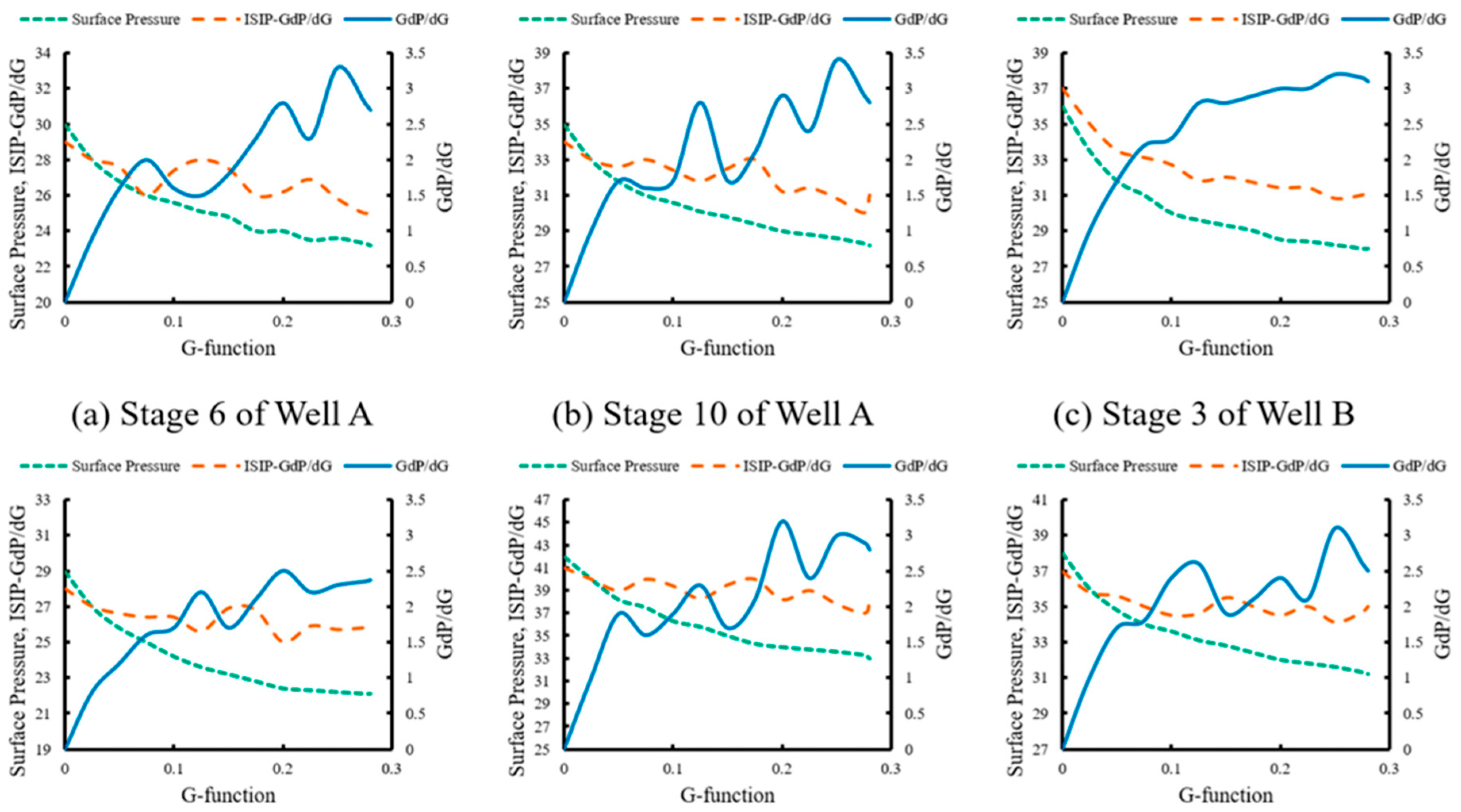
By plotting the relationship curves of the G-function with its first derivative and superposition derivative, fracture type and branch fracture count can be discriminated according to curve characteristics. The specific discrimination logic is as follows: if the first derivative exhibits a constant value and the superposition derivative curve substantially coincides with the pressure decline curve, it is determined that only a primary hydraulic fracture has formed, i.e., no branch fractures exist; if the first derivative shows fluctuations of small amplitude while the superposition derivative curve deviates from the pressure decline curve and presents a single upward convex morphology, it is determined that one natural fracture has been connected; if the first derivative exhibits significant fluctuations and the superposition derivative curve obviously deviates from the pressure decline curve prior to closure with multiple peaks, it is determined that multiple natural fractures have been connected, and the number of peaks is correlated with the branch fracture count.

The discrimination strategy outlined above, which infers the number of hydraulically connected natural fractures activated during fracturing from G-function derivative signatures, aligns with the method reported by Zhao et al. [16] for evaluating post-fracture complexity of hydraulically fractured wells in the Fuling gas field, lending independent support to the diagnostic criterion adopted in this work.

To render the above discrimination quantitative and reproducible, explicit peak-identification criteria are applied to the superposition derivative curve G·dP/dG prior to closure: a local maximum is identified as a valid peak only when its amplitude exceeds the adjacent trough values by more than 20% of the mean curve amplitude over the diagnostic window.

Consistent with conventional diagnostic approaches, heavy noise, sparse sampling, or incomplete shut-in records can smear derivative peaks and induce counting errors in the branch fracture count. To minimize this risk, all pressure decline data in this study were smoothed and screened for outliers prior to derivative computation, and fracturing stages with abnormally degraded data quality were excluded from the analysis. In addition, peaks emerging near the fracture closure point still cannot be resolved with complete unambiguity, such that the diagnosed branch fracture count bears an uncertainty of approximately ±1. Within the inversion workflow, this uncertainty merely causes expansion or narrowing of the candidate subspace and does not propagate into the quantitative estimates of the remaining fracture parameters.

Table 1. Basic reservoir physical properties of the study block.

Parameter	Well A	Well B	Well C
Horizontal section depth, m	2814–4291	2585–4085	3146–4602
Average Young’s modulus, GPa	36.19	45.19	52.3
Average Poisson’s ratio	0.22	0.33	0.23

and

Table 2. Operational parameters of hydraulic fracturing in the study block.

Parameter	Well A	Well B	Well C
Number of fracturing stages	17	21	23
Total fracturing fluid volume	24,946	23,460	34,962
Slickwater volume	20,582	21,320	35,026
Gel volume	6166	8450	1736
Total proppant volume	1125	1671	1340
100-mesh ceramic proppant	54	107	198
40/70 resin-coated sand	917	1321	1035
30/50 resin-coated sand	138	202	91
Pumping rate	10–14	12–14	12–14

present the basic physical properties and operational parameters of three wells in the study block. All subsequent sample database construction and case validation are based on data from this block.

Following the quantitative discrimination criteria described above, G-function analyses were conducted on six representative fracturing stages in the study block, and the results are presented in Figure 2. Specifically, for Stage 6 of Well A and Stage 7 of Well C, the first derivative curves of the G-function exhibit pronounced fluctuations prior to closure, while the superposition derivative curves deviate from the pressure decline curves and display three distinct peaks. Accordingly, these stages are determined to have connected three natural fractures, a branch fracture count N_b = 3. Similarly, Stage 10 of Well A and Stage 5 of Well C are identified to have connected four natural fractures, N_b = 4; Stage 3 of Well B shows no connection with natural fractures, N_b = 0; and Stage 7 of Well B is determined to have connected two natural fractures, N_b = 2. The diagnosed branch fracture count serves as a hard constraint in the subsequent fracture morphology inversion, effectively narrowing the parameter optimization space and preventing inversion results from deviating from geological and engineering reality.

2.2. Mathematical Model for Fracture Morphology Inversion and CNN-LSTM Hybrid Neural Network Architecture

Based on the G-function diagnosis that determines the branch fracture count, the complete geometric morphology and flow parameters of the fractures need to be further inverted. In this study, fracture morphology is simplified into five key parameters: fracture length L_f (m), fracture width W_f (mm), fracture height H_f (m), fracture conductivity F_cD (μm²·cm), and branch fracture count N_b (dimensionless). These parameters encompass two core dimensions of fracture spatial distribution and flow capacity, reflecting both the geometric characteristics of fractures and their conductivity to hydrocarbon flow [17]. Among them, the branch fracture count Nb is directly prescribed by the G-function diagnosis, while the remaining four-dimensional parameters are determined through production matching inversion using the CNN-LSTM model.

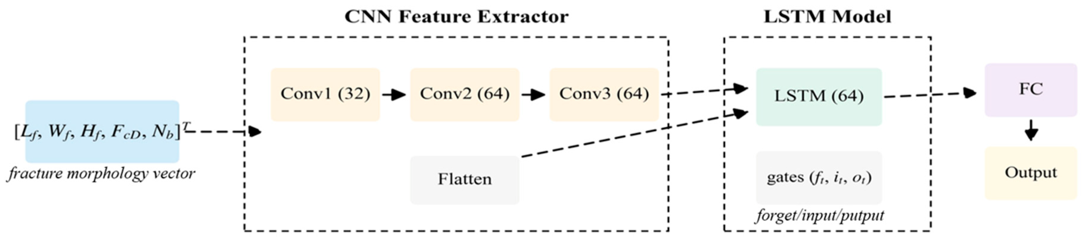
Figure 3 illustrates the CNN-LSTM hybrid neural network architecture. The input layer receives the standardized five-dimensional fracture morphology parameter vector [L_f, W_f, H_f, F_cD, N_b]^T. After progressive layer-wise abstraction by the CNN spatial feature extraction module, the resulting features are broadcast to every time step and concatenated with the normalized production time coordinate to form the input sequence of the LSTM temporal modeling module, which models the temporal evolution of the production dynamics over the production period. The predicted cumulative production over the period is then output through the fully connected layer. The mathematical formulations for each module are presented as follows.

(1)

CNN Spatial Feature Extraction Module

Let the input fracture morphology parameter vector be X = [L_f, W_f, H_f, F_cD, N_b]^T. The output feature map H(l) of the l-th convolutional layer can be expressed as

$$H_{i,j}^{(l)}=f({\displaystyle \sum _m{\displaystyle \sum _n{W}_{m,n}^{(l)}}}\cdot H_{i+m,j+n}^{(l-1)}+b^{(l)})$$

(4)

where W^(l) denotes the convolutional kernel weight matrix; b^(l) is the bias term; and f(·) represents the ReLU activation function, i.e., f(x) = max (0, x). The first convolutional layer employs 32 convolutional kernels of size 1 × 3 to extract local correlation features between adjacent parameters. The second and third layers each adopt 64 convolutional kernels; through progressive layer-wise abstraction, high-order coupling relationships among fracture parameters are extracted [18]. After three convolutional layers, the feature maps are converted into a one-dimensional feature vector via a flattening operation, serving as the spatial input to the LSTM module.

Mathematically, the parameter vector is arranged as a one-dimensional feature channel, and each kernel of size 1 × 3 slides along this channel with unit stride, computing at each position a learnable weighted combination of three adjacent parameters. It should be emphasized that the parameter vector is not treated as a time series: the one-dimensional convolution is employed solely as a local feature interaction operator, which is mathematically equivalent to a locally connected layer with weight sharing, that is, a structured multilayer perceptron with local receptive fields, and no temporal meaning is attached to the parameter order; the temporal modeling of the production data is delegated entirely to the LSTM module, whose input is the actual production time series. Physically, the arrangement of the parameter vector is not arbitrary, because the three window positions of the 1 × 3 kernel correspond exactly to three physically meaningful parameter groups: the first window [L_f, W_f, H_f] jointly defines the fracture geometry and thus the stimulated reservoir volume; the second window [W_f, H_f, F_cD] combines the flow cross-section with the fracture conductivity and thus governs the deliverability of the main fracture; and the third window [H_f, F_cD, N_b] characterizes the fracture complexity, in which the branch fracture count Nb defines the topological complexity of the network, while the main-fracture height and conductivity determine how effectively this complexity is converted into production. From the learning perspective, restricting feature interaction to physically coupled neighbors amounts to imposing a physical prior on the model: a fully connected layer would allow arbitrary parameter pairs to interact freely, whereas the 1 × 3 convolution permits preferential interaction only among parameters with direct physical coupling; the associated reduction in trainable parameters further alleviates overfitting given the limited size of the training database (600 samples). The favorable generalization performance on the independent test set (Section 3.2.2) corroborates the appropriateness of this architectural choice.

(2)

LSTM Temporal Modeling Module

LSTM controls the flow and forgetting of information through three gating mechanisms: the forget gate f_t, the input gate i_t, and the output gate o_t. Let x_t denote the input at time t denote the network input at time step t as x_t = [z; τ_t], where z is the flattened spatial feature vector produced by the CNN module and is shared by all time steps, and τ_t is the normalized production time coordinate; the production period is thereby unrolled into a sequence of T time steps, along which the LSTM models the temporal evolution of the production dynamics. The hidden state h_t−1 and cell state C_t−1 from the previous time step are used in the following gate computations. The computation formulas for each gate are then expressed as

$$f_t=\sigma (W_f\cdot [h_{t-1},x_t]+b_f)$$

(5)

$$i_t=\sigma (W_i\cdot [h_{t-1},x_t]+b_i)$$

(6)

$${\tilde{C}}_t=\tanh (W_C\cdot [h_{t-1},x_t]+b_C)$$

(7)

$$C_t=f_t\odot C_{t-1}+i_t\odot {\tilde{C}}_t$$

(8)

$$o_t=\sigma (W_o\cdot [h_{t-1},x_t]+b_o)$$

(9)

$$h_t=o_t\odot \tanh (C_t)$$

(10)

where σ(·) denotes the Sigmoid activation function; tanh(·) denotes the hyperbolic tangent function; ⊙ represents the Hadamard product (element-wise multiplication); and W and b are the weight matrices and bias terms for each gate, respectively. The forget gate determines the retention ratio of the cell state from the previous time step, the input gate controls the update magnitude of the current candidate state, and the output gate regulates the output intensity of the hidden state. Through this gating mechanism, LSTM effectively avoids the vanishing gradient problem faced by conventional RNNs when processing long sequences.

(3)

Fully Connected Layer and Production Output

The hidden state at the final time step, which aggregates the temporal production dynamics over the entire production period, is mapped to the predicted cumulative production via the fully connected layer:

$$\widehat{y}=W_{fc}\cdot h_T+b_{fc}$$

(11)

where h_T is the hidden state at the final time step, which aggregates the production dynamics over the entire production period; W_fc and b_fc are the weight matrix and bias term of the fully connected layer, respectively; and ŷ is the predicted cumulative gas production over the production period, which serves as the target variable of the subsequent inversion.

(4)

Loss Function and Adam Optimizer

Model training employs mean squared error (MSE) as the loss function to measure the deviation between predicted and actual production values:

$$L_{\mathrm{MSE}}={\displaystyle \frac{1}{N}}{\displaystyle \sum _{i=1}^N(}{y}_i-{\widehat{y}}_i{)}^2$$

(12)

where N denotes the number of samples; y_i is the actual production; and ŷ_i is the model-predicted production.

The Adam (Adaptive Moment Estimation) optimizer is employed for parameter updating. Adam combines the advantages of the momentum method and RMSProp, adaptively adjusting the learning rate for each parameter by computing the first moment estimate (mean) and second moment estimate (uncentered variance) of the gradients. The parameter update rules are expressed as

$$m_t={\beta }_1{m}_{t-1}+(1-{\beta }_1)g_t$$

(13)

$$v_t={\beta }_2{v}_{t-1}+(1-{\beta }_2)g_t^2$$

(14)

$${\widehat{m}}_t=m_t/(1-{\beta }_1^t),\hspace{0.33em}{\widehat{v}}_t=v_t/(1-{\beta }_2^t)$$

(15)

$${\theta }_t={\theta }_{t-1}-\eta \cdot {\widehat{m}}_t/\sqrt{{\widehat{v}}_t+\epsilon }$$

(16)

where g_t is the gradient at time t; mt and v_t are the first and second moment estimates of the gradient, respectively; β₁ = 0.9 and β₂ = 0.999 are the decay coefficients; η = 0.001 is the initial learning rate; and ε = 10⁻⁸ is a small constant to prevent division by zero.

3. Model Testing and Application

3.1. Construction of the Fracture–Production Mapping Sample Database

A three-dimensional gas–water two-phase reservoir model is built using the CMG simulator based on the average reservoir parameters of the target block (

Table 3. Key input parameters of the CMG numerical simulation model.

Parameter	Value
Pressure coefficient	0.93
Porosity, %	10.97
Permeability, mD	1.69
Initial reservoir pressure, MPa	27.91
Interlayer thickness, m	6
Young’s modulus, MPa	44,560
Poisson’s ratio	0.260
Maximum horizontal principal stress, MPa	50.1
Minimum horizontal principal stress, MPa	42.5
Leakoff coefficient, m/min1/2	5.76 × 10−4
Gas saturation, %	62

). The model domain adopts a grid dimension of 400 m × 400 m × 200 m. The reservoir is assumed to be homogeneous, with uniform initial formation pressure and water saturation distribution. The key geomechanical and fluid flow parameters assigned in the model are summarized in Table 3.

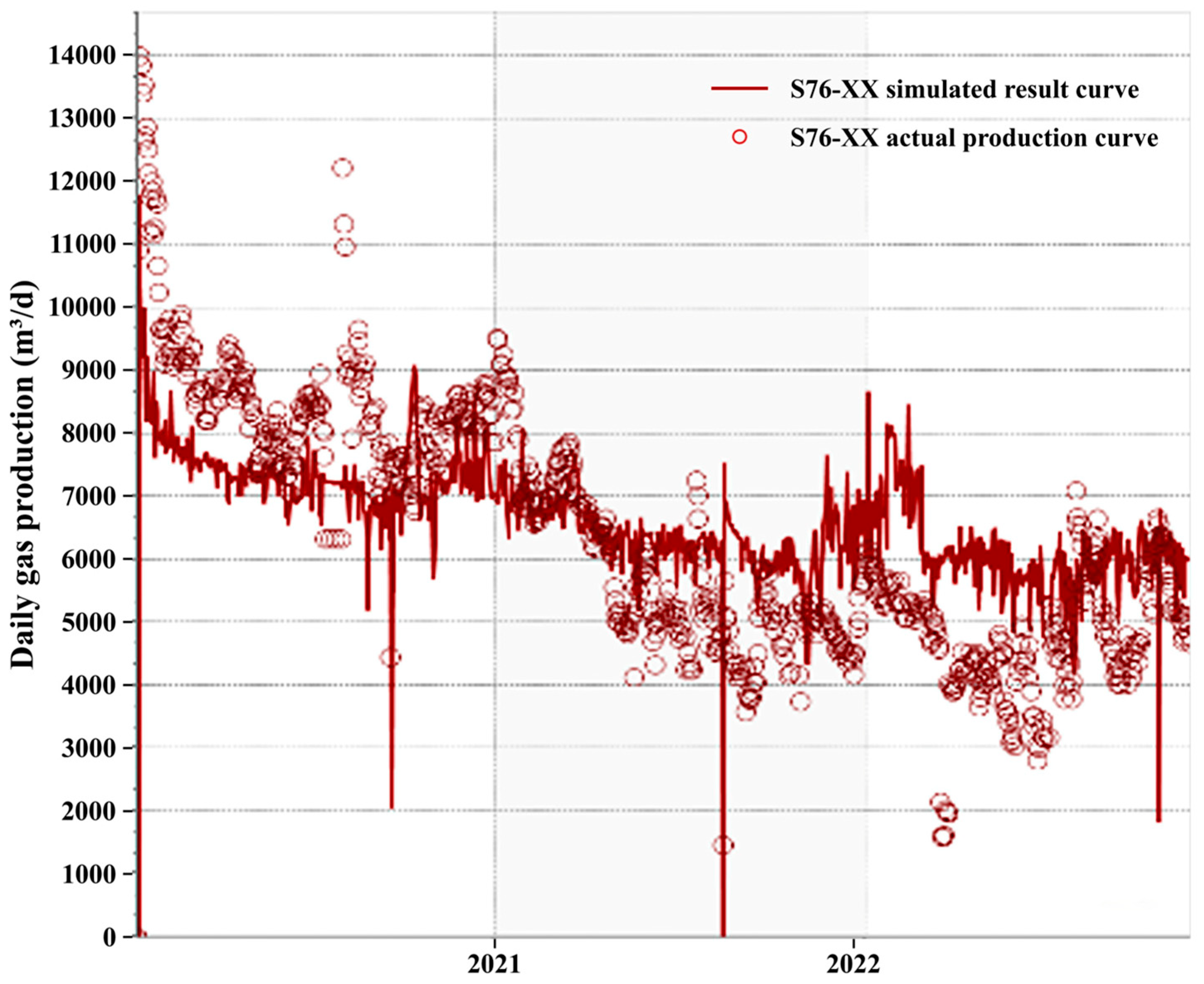
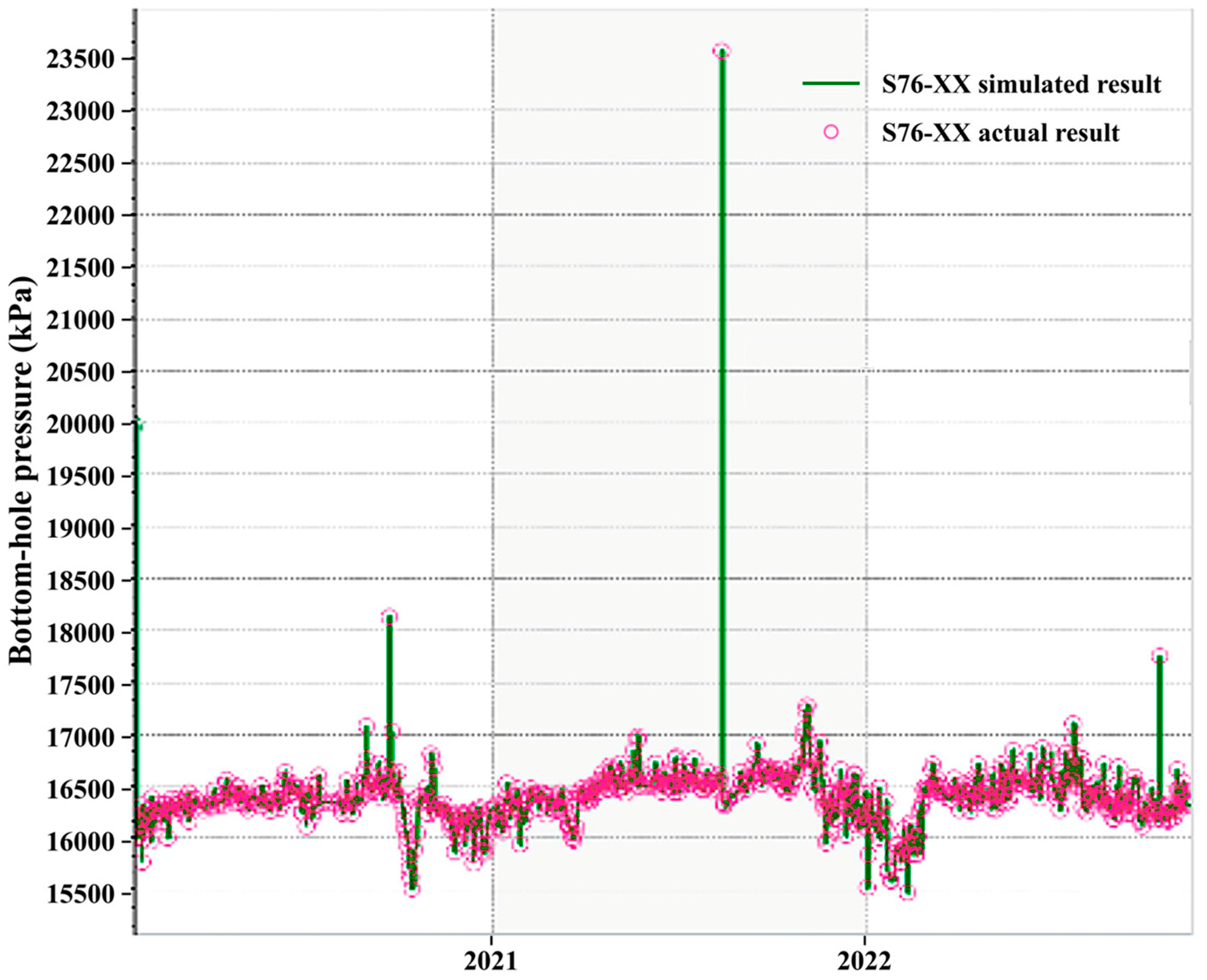
Prior to sample generation, the simulation model was validated against the actual production history of Well S76-XX in the study block. The corresponding history-matching results for daily gas production and bottom-hole flowing pressure are presented in Figure 4 and Figure 5. The simulated gas production reproduces the field measurements with a relative error below 10%, which confirms that the model is adequate for constructing the training database.

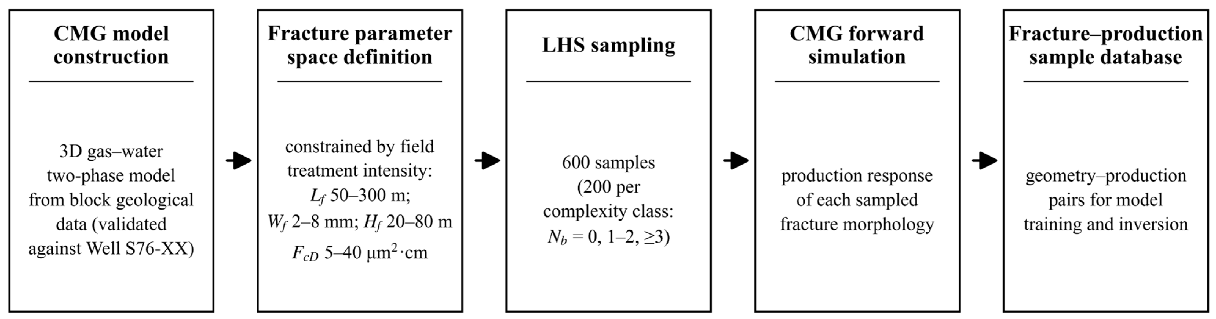
Within this database, the branch fracture count N_b diagnosed from the G-function analysis serves as the hard constraint that fixes the topological complexity of each sample. To reduce the computational cost of database construction while enhancing the capability to characterize fracture systems of varying complexity, the samples are organized into three complexity levels according to N_b: N_b = 0, N_b = 1–2, and N_b ≥ 3.

For the fracture morphology parameters, the value ranges were determined comprehensively from regional geological data, namely fracturing operation records: fracture half-length of 50–300 m, fracture width of 2–8 mm, fracture height of 20–80 m, and conductivity of 5–40 μm²·cm.

Based on this validated model, a total of 600 samples were generated, with 200 samples for each complexity level. Within each level, the Latin hypercube sampling (LHS) method was employed to draw parameter combinations from the above ranges, ensuring that the samples cover the complete parameter interval without sampling bias; owing to its space-filling property, the four continuous parameters exhibit approximately uniform marginal distributions over their respective ranges, and no spurious correlations are introduced among the parameters. Each sampled fracture morphology was then forward-simulated with the CMG model to obtain its production response. The overall workflow of the sample database generation is illustrated in Figure 6.

The statistical characteristics of the generated database are summarized in

Table 4. Statistical characteristics of the generated sample database.

Parameter	Min	Max	Mean	Std
Fracture half-length, m	50.00	300.00	175.00	72.23
Fracture width, mm	2.00	8.00	5.00	1.73
Fracture height, m	20.00	80.00	50.00	17.33
Fracture conductivity, μm2·cm	5.00	40.00	22.50	10.11
Monthly cumulative gas production, t	34.60	258.30	109.70	64.58

. For each continuous parameter, the sample mean and standard deviation are close to the theoretical values of the corresponding uniform distribution. The LHS samples uniformly cover the prescribed parameter space and introduce no spurious correlations. The monthly cumulative gas production of the 600 samples ranges from 34.6 t to 258.3 t, with a mean of 109.7 t, which is consistent with the production level of the study block.

The construction of the sample database enables systematic matching between various fracture morphologies and their corresponding production responses. For each branch fracture complexity type, the database encompasses typical parameter combinations under that complexity category and their associated production responses, thereby providing a data foundation for subsequent model training and production inversion. In practical inversion applications, once an actual production target is given, a sample subset belonging to the same branch fracture count category is first screened from the database. The matching degree between the predicted production and actual production is then computed for each sample as (1 − |predicted value − actual value|/actual value), and the parameters of the sample with the highest matching degree are adopted as the inversion result.

It should be acknowledged that the synthetic samples are generated from a homogeneous reservoir model, whereas real reservoirs are heterogeneous, and a distribution gap therefore inevitably exists between the LHS samples and real-field data. Three measures are adopted to mitigate this gap. First, the parameter ranges are bounded by the geological data and fracturing operation records of the study block rather than chosen arbitrarily, so that the sampled space envelopes the fracture morphologies that can actually develop under the local in situ stress and operational conditions. Second, the branch fracture count diagnosed from the G-function analysis restricts the inversion to the subset of samples sharing the same topological complexity as the target stage, which further narrows the candidate space toward the actual fracture system. Third, the simulation model is anchored to the field through history matching with Well S76-XX prior to sample generation, so that the synthetic production responses are calibrated against real production behavior. The inverted parameters should therefore be interpreted as equivalent fracture parameters that reproduce the observed production under the homogeneous model assumption, rather than as a point-by-point reconstruction of the heterogeneous fracture network. The merit of this work lies in the batch inversion of post-fracturing fracture morphologies for multiple wells using the established sample database. Explicit incorporation of reservoir heterogeneity into the sample generation workflow will be considered in future research.

3.2. Model Training and Multi-Branch Fracture Validation

Samples were randomly partitioned into training, validation, and test sets at a ratio of 7:2:1. A stratified sampling strategy was employed during partitioning to ensure that the proportion of samples with different branch fracture counts in each subset remained consistent with the overall dataset, thereby avoiding model bias arising from sample imbalance. The constructed CNN-LSTM neural network was trained for 200 iterations, with mean squared error serving as the loss function and the Adam optimizer adopted at an initial learning rate of 0.001.

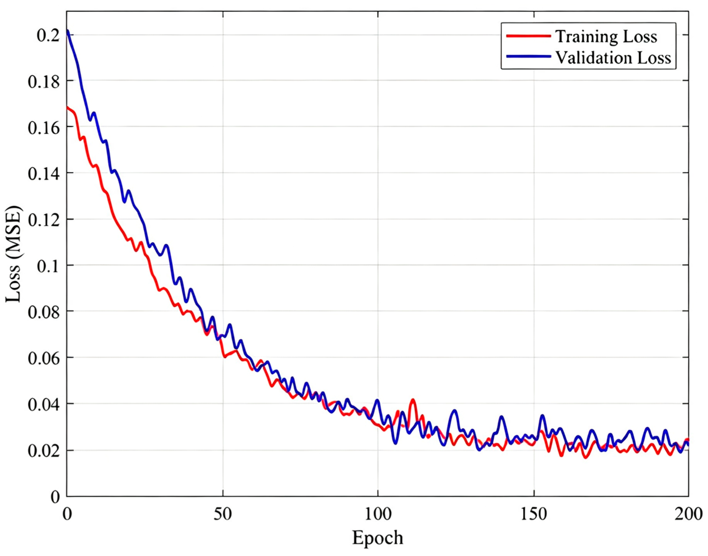
During the training process, an early stopping mechanism with a patience of 20 epochs was adopted to prevent overfitting: training was terminated once the validation loss failed to decrease for 20 consecutive epochs, and the network weights corresponding to the lowest validation loss were retained as the final model. The final model achieved a mean squared error of 0.023 on the training set and 0.031 on the validation set.

The hyperparameters of the network were determined by grid search on the validation set prior to the final training. The search space included the number of convolutional kernels per layer (16, 32, 64, or 128), the number of LSTM units (32, 64, 128, or 256), the initial learning rate (1 × 10⁻², 1 × 10⁻³, or 1 × 10⁻⁴), and the batch size (16, 32, or 64); the kernel size (1 × 3) and the number of convolutional layers (three) were fixed according to the physical considerations discussed in Section 2.2. Each candidate configuration was trained under the same early stopping rule, and the configuration yielding the lowest validation loss was selected, namely, 32, 64, and 64 kernels in the three convolutional layers, 64 LSTM units, an initial learning rate of 1 × 10⁻³, and a batch size of 32. Larger configurations (for example, 128 kernels per layer or 128–256 LSTM units) brought no further reduction in the validation loss but a visibly widened gap between the training and validation losses, indicating aggravated overfitting on the 420-sample training set, whereas smaller configurations underfitted the coupling relationships among the fracture parameters.

Figure 7 illustrates the evolution of loss curves during the training process of the CNN-LSTM model. In the early training stage (the first 50 iterations), both the training loss and validation loss decrease rapidly, indicating that the model is effectively learning the mapping relationship between fracture morphology and production. In the middle training stage (50–150 iterations), the rate of loss decline decelerates, and the validation loss fluctuates around 0.035 with no evident signs of overfitting. In the late training stage (150–200 iterations), the loss tends to stabilize, with the training loss remaining around 0.023 and the validation loss around 0.031, signifying that the model has reached a converged state. The validation loss reached its minimum at approximately the 180th iteration, and training was terminated at the 200th iteration under the early stopping rule.

3.2.1. Production Prediction Accuracy for Different Branch Fracture Counts on the Training Set

To systematically evaluate the model’s fitting capability across fracture networks of varying complexity, the prediction accuracy on the training set is analyzed and categorized by branch fracture count. The statistical results are presented in

Table 5. Validation of prediction performance for different branch fracture counts on the training set.

Branch Fracture Count, Nb	R2	MAE, t/month	RMSE, t/month	MAPE, %
0	0.96	2.1	3.5	3.2
1–2	0.94	3.2	5.1	4.8
≥3	0.85	4.5	7.2	7.3

.

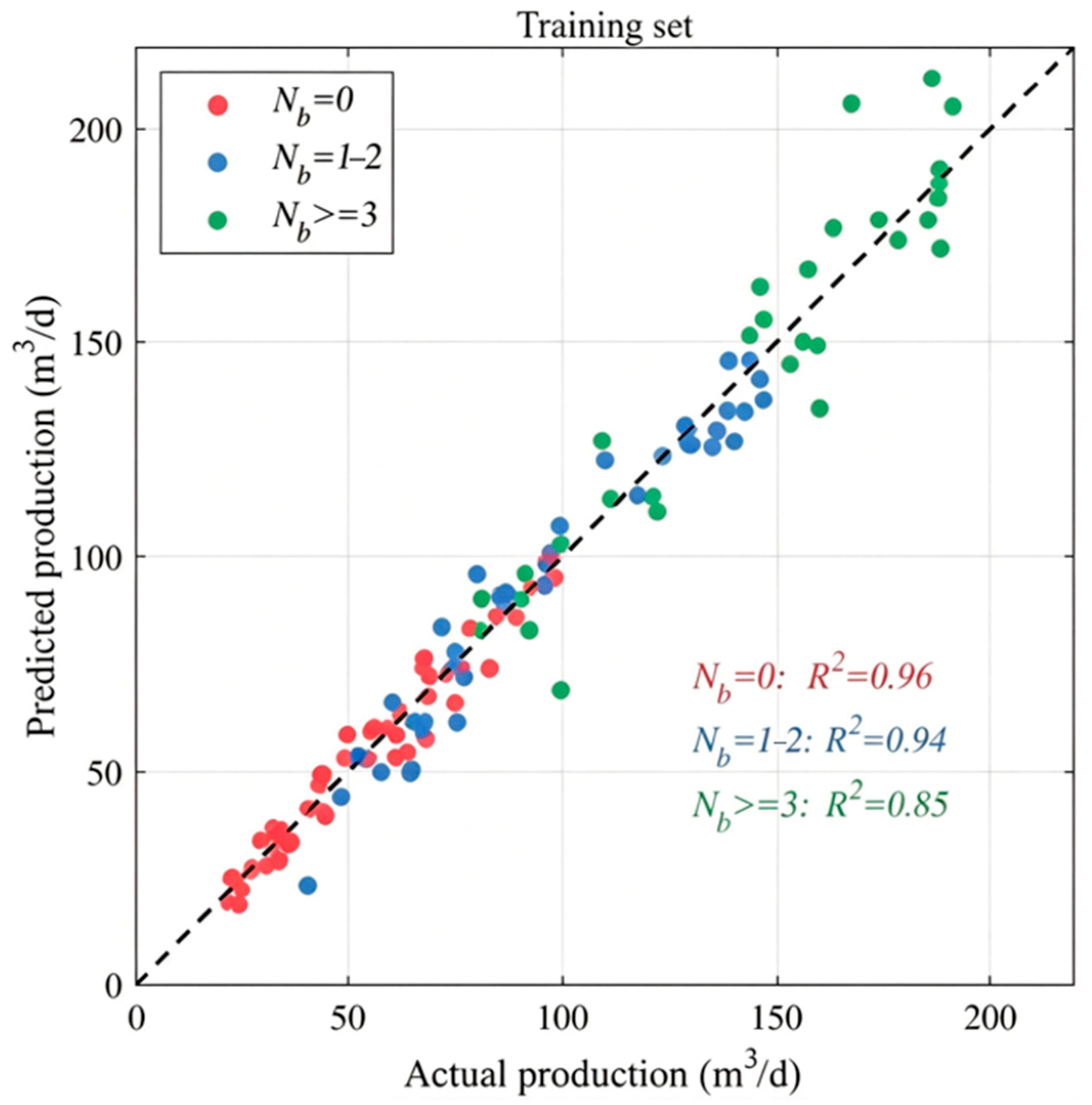
As shown in Table 5, the prediction accuracy of the model on the training set exhibits a gradually decreasing trend with increasing branch fracture count. When N_b = 0, the fracture morphology is a simple bi-wing fracture with well-defined parameter coupling relationships; the coefficient of determination R² of the model reaches 0.96, and the mean absolute error MAE is merely 2.1 t/month. When N_b ≥ 3, the fracture network presents a complex branching or mesh-like structure, and the nonlinear coupling among parameters is significantly enhanced. The model coefficient of determination R² decreases to 0.85, and the MAE increases to 4.5 t/month. This is because the increase in branch fracture count leads to a sharp rise in the dimensionality and complexity of the fracture morphology parameter space, making the nonlinear mapping relationships that the CNN-LSTM network needs to learn more intricate; under the same network architecture, the fitting difficulty increases, and the prediction error grows accordingly.

Figure 8 presents the production prediction results on the training set for different branch fracture counts. For samples with N_b = 0, the predicted and actual production values are highly concentrated near the 1:1 diagonal line, with extremely low data dispersion. As the branch fracture count increases, the data dispersion grows slightly, yet the overall linear correlation remains favorable, indicating that the model possesses good fitting capability for the training samples.

3.2.2. Production Prediction Accuracy for Different Branch Fracture Counts on the Test Set

To validate the generalization capability of the model, independent validation was conducted using test set samples that were not involved in the training process, and the results are presented in

Table 6. Validation of prediction performance for different branch fracture counts on the test set.

Branch Fracture Count, Nb	R2	MAE, t/month	RMSE, t/month	MAPE, %
0	0.93	4.1	6.3	6.2
1–2	0.84	5.5	8.8	9.1
≥3	0.78	6.5	10.2	10.8

.

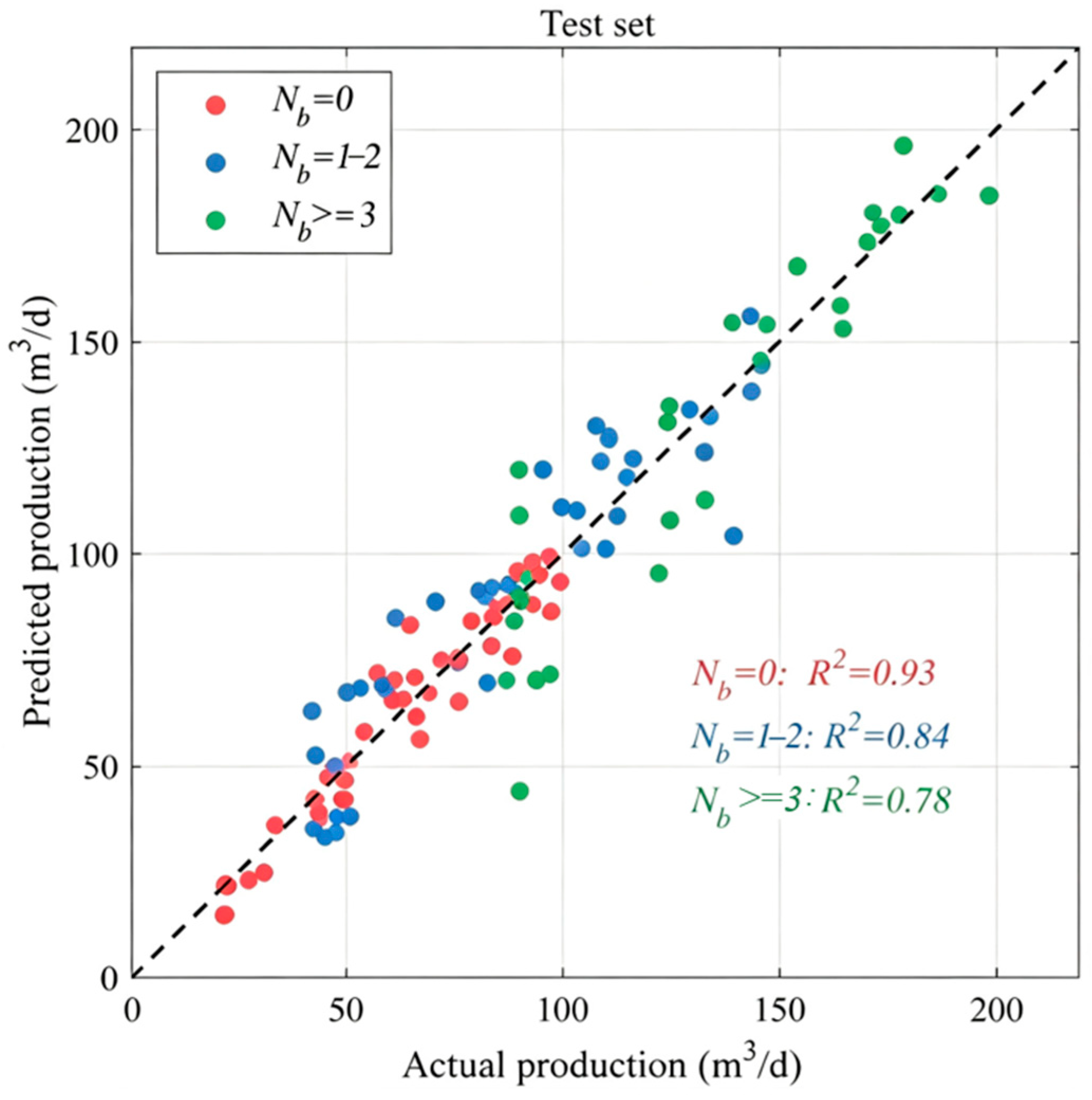
As shown in Table 6, the test set exhibits the same trend that prediction accuracy decreases with increasing branch fracture count. When N_b = 0, the test set R² is 0.93; when N_b ≥ 3, the test set R² drops to 0.78. In addition, the overall accuracy evaluation metrics on the test set are as follows: the coefficient of determination R² reaches 0.85, the MAE is 5.37 t/month, the RMSE is 8.43 t/month, and the MAPE is 8.7%.

Figure 9 presents the validation of production prediction performance on the test set. Although the test set samples were not involved in the training process, the model maintains high prediction accuracy, with data points generally distributed along the 1:1 diagonal line. The prediction deviation is particularly small in the low-to-medium production range, verifying the generalization capability of the CNN-LSTM model for the fracture morphology to production mapping relationship.

In field engineering, a prediction error within 10% is commonly accepted for production forecasting and history matching of fractured gas wells [19], where the combined uncertainty of reservoir description, measurement, and operational conditions typically limits the practical predictability of well performance to within 10–15%. The 8.7% MAPE of the present model therefore satisfies this criterion; its acceptability nevertheless depends on the intended application. For post-fracturing evaluation and fracture design optimization, which are the primary objectives of the present framework, an error of this magnitude is adequate, because the ranking of candidate fracture geometries and the identification of the controlling parameters are preserved. For applications that are more sensitive to absolute production levels, such as reserve estimation and long-term production forecasting, the prediction should be interpreted together with the uncertainty bounds reported below rather than as a single deterministic value.

To quantify the predictive uncertainty, a 90% prediction interval was constructed from the empirical distribution of the test set residuals. For the cumulative gas production, the resulting half-width is approximately 10.2 t, and 90.2% of the test samples are predicted within ±10% of the actual cumulative production, indicating that the uncertainty estimate is well calibrated.

The prediction error varies systematically with both the production level and the fracture complexity. When the test samples are divided into high- and low-production subsets by a threshold of 100 t in the monthly cumulative production, the relative error is markedly lower in the high-production subset than in the low-production subset: the MAPE is 7.0% for samples with a cumulative production above 100 t, but rises to 11.3% for those below this threshold, because an absolute deviation of comparable magnitude corresponds to a larger relative error when the production base is smaller. With respect to fracture complexity (Table 6), the MAPE increases from 6.2% for N_b = 0 to 9.1% for N_b = 1–2 and 10.8% for N_b ≥ 3, reflecting the stronger nonlinear parameter coupling in complex fracture networks. The slight excess over the 10% tolerance in the most complex class does not compromise the practical use of the framework.

The decrease in prediction accuracy with increasing branch fracture count is a normal phenomenon rather than a deficiency of the model. A larger Nb corresponds to a more complex fracture network, for which the number of possible fracture morphologies that can match a given production response grows rapidly; the parameter-to-production mapping is therefore intrinsically less constrained, and the prediction accuracy decreases accordingly. It should also be noted that the absolute error increases only moderately (the MAPE rises from 6.2% for Nb = 0 to 10.8% for Nb ≥ 3), and the branch fracture count supplied by the G-function diagnosis restricts the inversion to the correct complexity class, within which the relative ranking of candidate geometries remains reliable.

To position the proposed model against standard machine learning approaches, five widely used baselines—a multilayer perceptron (MLP), a random forest (RF), LightGBM, XGBoost, and a pure LSTM network without the convolutional module—were trained and evaluated on the same sample database with the same input parameters and the same training/validation/test partitioning; the hyperparameters of all baselines were tuned by grid search with fivefold cross-validation on the training set. The results are summarized in

Table 7. Performance comparison of the proposed CNN-LSTM model with standard machine learning baselines on the test set.

Model	R2	MAE, t/month	RMSE, t/month	MAPE, %
CNN-LSTM (this study)	0.85	5.4	8.4	8.7
MLP	0.80	6.6	10.2	12.3
LightGBM	0.80	6.5	10.1	11.9
Pure LSTM	0.82	6.3	9.8	11.5
Random forest	0.79	6.8	10.5	12.8
XGBoost	0.83	6.1	9.5	11.2

. All five baselines attain reasonable accuracy, with test set R² values between 0.79 and 0.83, indicating that the fracture–production mapping is learnable by mainstream machine learning methods; the proposed CNN-LSTM model nevertheless achieves the best performance on every metric, with an overall test set R² of 0.85 and a MAPE of 8.7%. In particular, the pure LSTM, from which the convolutional module is removed, exhibits a visible performance drop relative to the full model (R² = 0.82 versus 0.85), indicating that the convolutional module contributes a gain beyond what temporal modeling alone can provide; this is consistent with the architectural analysis in Section 2.2, where the 1 × 3 convolution is shown to provide an effective physical inductive bias, while the LSTM module captures the temporal production dynamics.

3.2.3. Model Interpretability and Physical Consistency Analysis

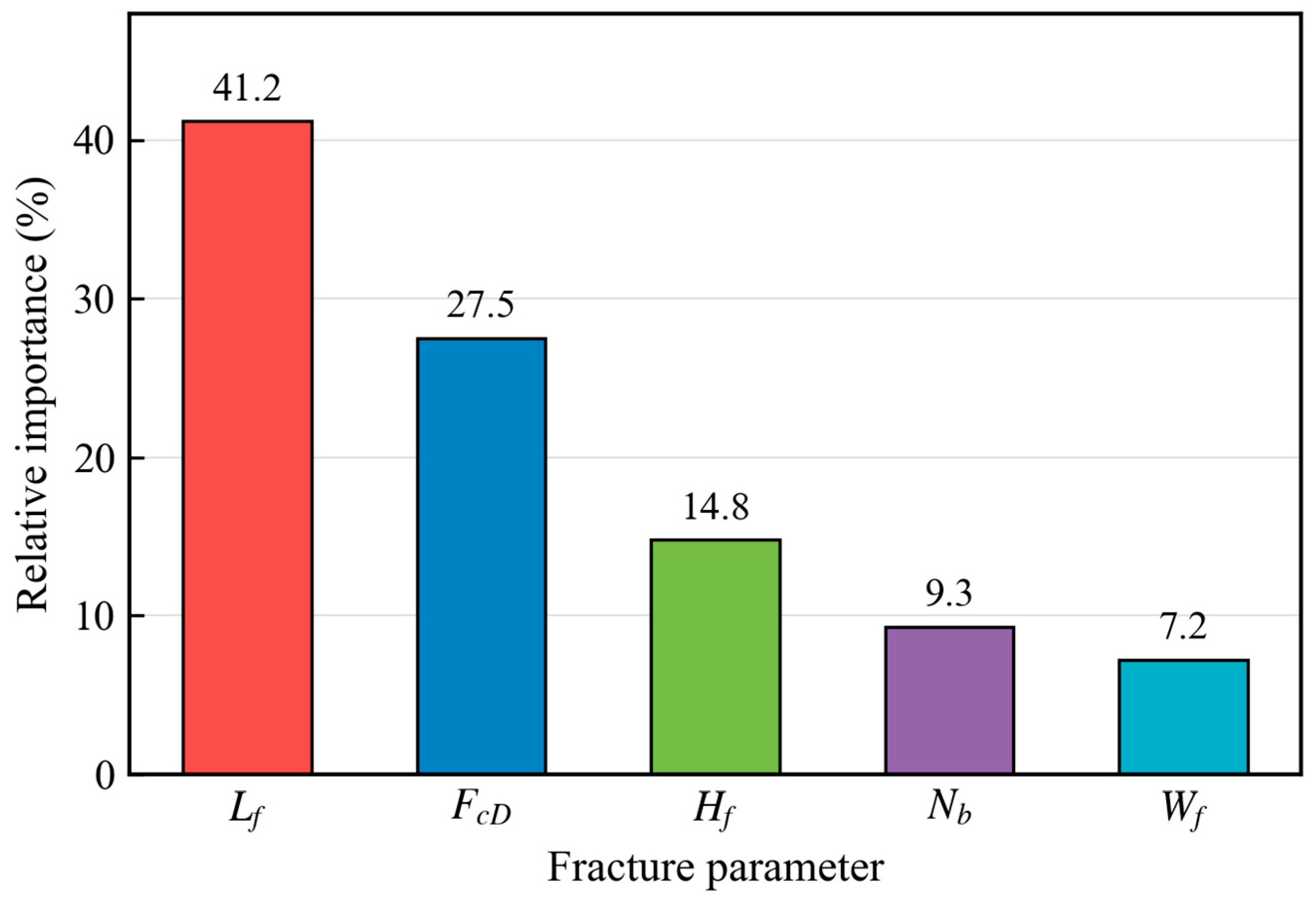
To assess whether the relationships learned by the CNN-LSTM model are physically plausible rather than artifacts of purely data-driven fitting, a permutation feature importance analysis was first conducted on the trained network. For each input parameter, its values across the test set samples were randomly reassigned among the samples while the remaining parameters were kept intact, thereby destroying the correspondence between that parameter and the true production response; the resulting decrease in R², averaged over 30 permutations with different random seeds, was taken as the importance score of that parameter. This model-agnostic measure is equivalent in spirit to SHAP-based interpretations.

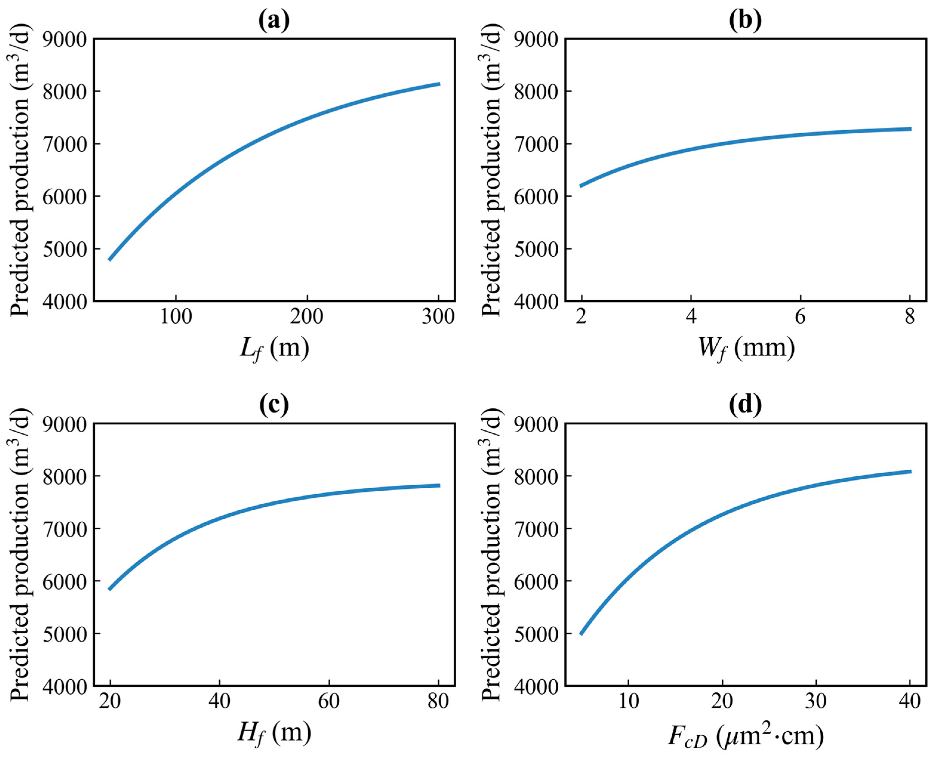
The resulting ranking (Figure 10) shows that the fracture half-length and fracture conductivity dominate the production prediction, accounting for 41.2% and 27.5% of the total importance, respectively, followed by the fracture height (14.8%), the branch fracture count (9.3%), and the fracture width (7.2%). Partial dependence curves (Figure 11), obtained by sweeping each parameter over its full range with the others fixed at their medians, show that the predicted production increases monotonically with all four geometric parameters, with diminishing marginal gain in every case: rising steeply before flattening for the half-length and conductivity, saturating once the pay interval is covered for the height, and climbing rapidly at small widths but flattening later for the width.

These trends agree with the physical understanding of fracture–production relationships: longer and more conductive fractures enlarge the stimulated reservoir volume and reduce flow resistance, though the incremental benefit declines near the drainage limit of the well; height growth ceases to help once the pay interval is covered; and widening an already sufficiently conductive fracture brings little additional gain. This result indicates that the G-function-constrained CNN-LSTM model captures physically plausible fracture–production mappings rather than merely fitting noise.

3.3. Model Application

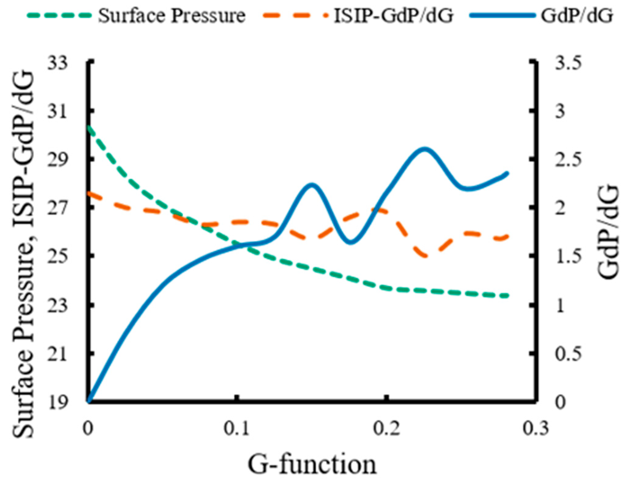
Taking the test stage of Well X in the target block as the engineering application object, the practical effectiveness of the proposed method is validated. First, the G-function method is applied to analyze the pressure decline curve of this stage. As shown in Figure 12, the first derivative curve of the G-function exhibits pronounced fluctuations prior to closure, while the superposition derivative curve deviates from the pressure decline curve and forms two distinct peaks. According to the discrimination criteria presented in Section 2.1, this stage is determined to have connected two natural fractures, i.e., a branch fracture count N_b = 2. This diagnostic result serves as a hard constraint in the inversion process, directly restricting the search to the N_b = 1–2 category subset in the sample database.

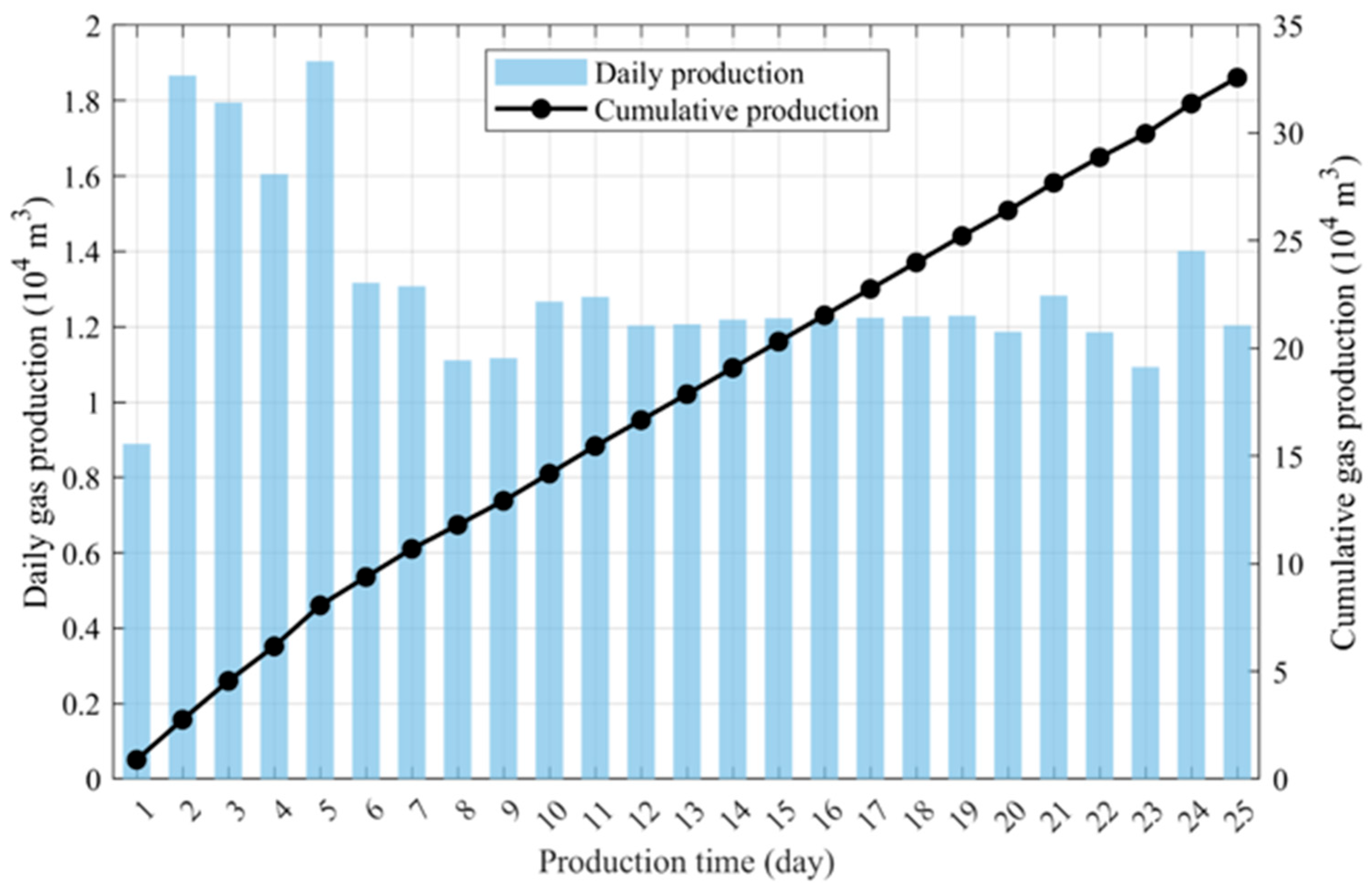
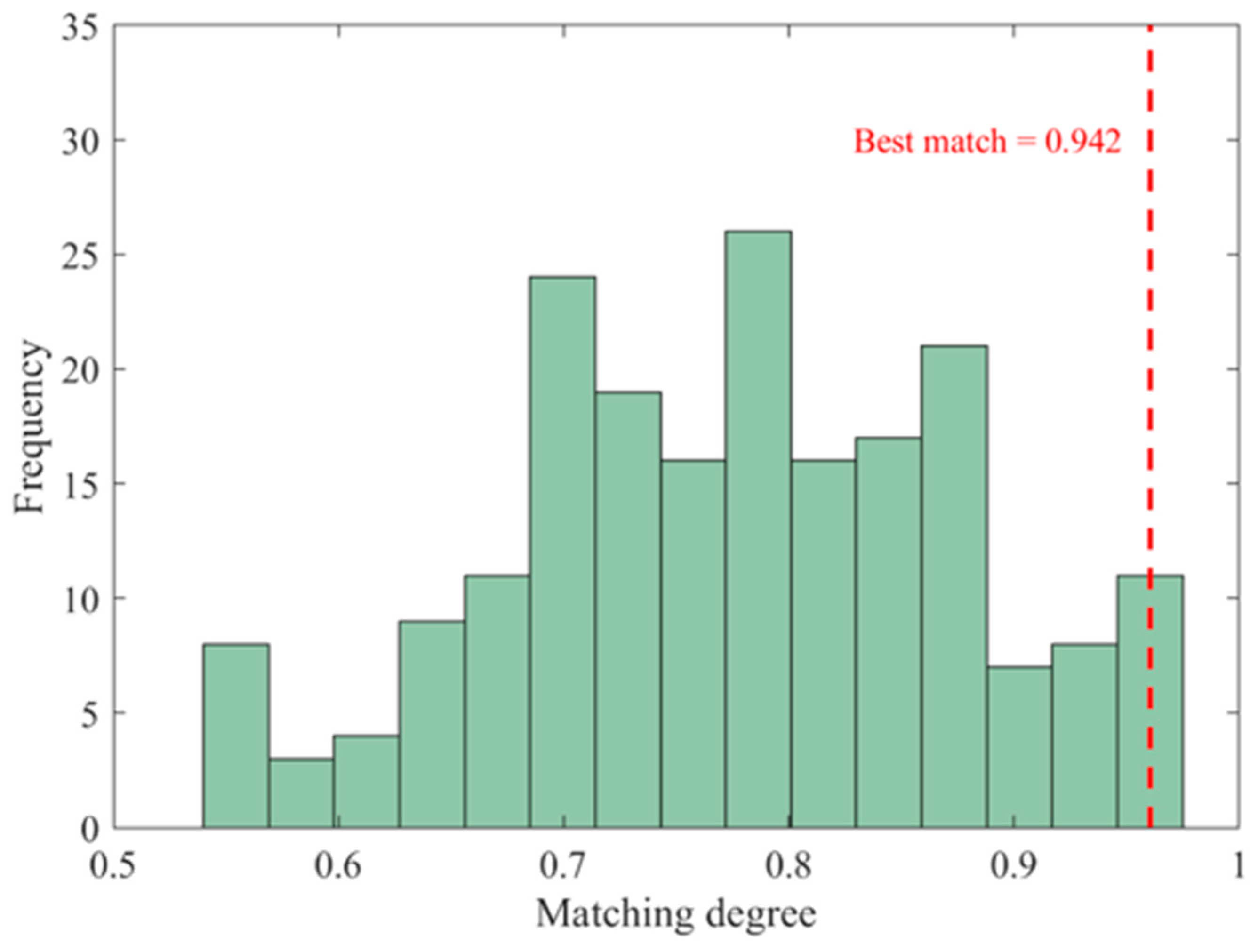
Based on the CNN-LSTM model and under the constraint of N_b = 2, the cumulative 25-day actual production data of the test stage are employed as the target constraint for inversion. Fracture morphology parameter combinations [L_f, W_f, H_f, F_cD, N_b]^T satisfying the condition are randomly generated within the parameter space, and the matching degree is calculated against the actual cumulative gas production of 32.5679 × 10⁴ m³. The production curve and matching degree distribution for the test stage are shown in Figure 13 and Figure 14, respectively. The matching degrees of most candidate combinations are concentrated in the range of 0.82–0.92, exhibiting an approximately normal distribution, with the peak located near 0.87; only a small number of combinations exceed 0.94. The parameter combination with the highest matching degree is screened out: fracture half-length 286 m, width 4.8 mm, height 64 m, and conductivity 16.5 μm²·cm, corresponding to a predicted cumulative gas production of 31.42 × 10⁴ m³ over 25 days, achieving a matching degree of 0.942 against the actual production of 32.5679 × 10⁴ m³.

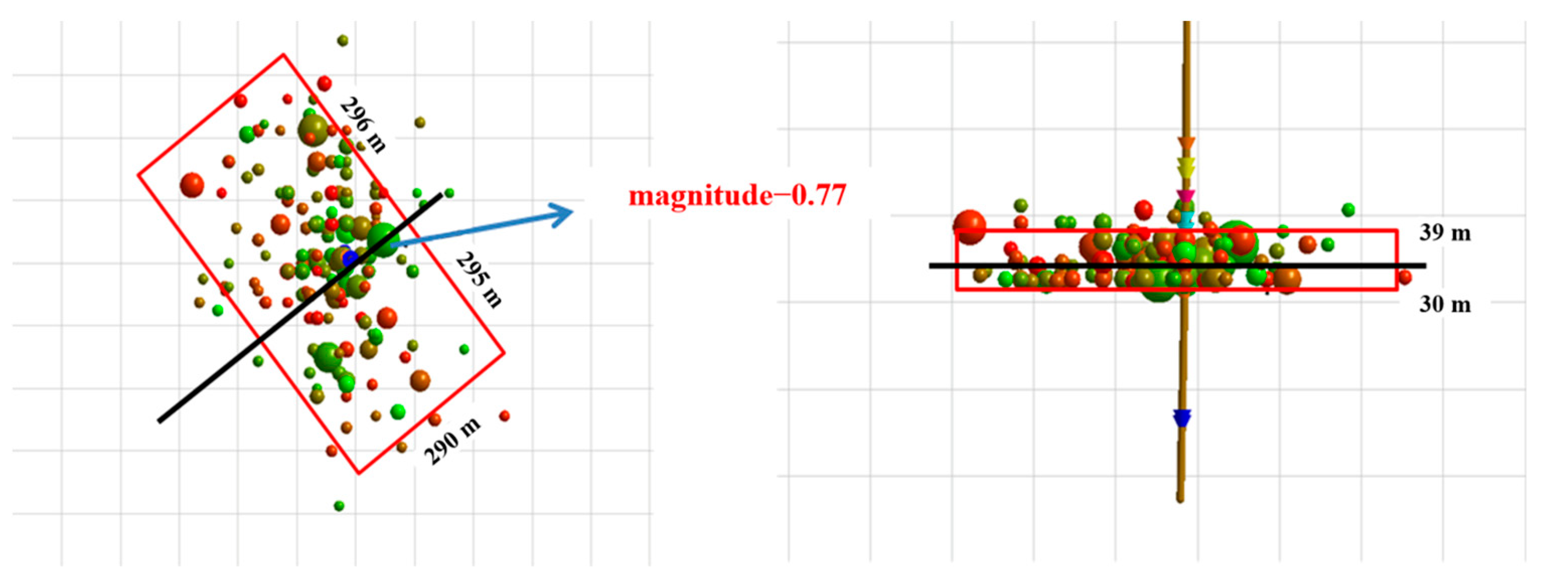
From the validation results, the inverted fracture half-length (286 m) is in excellent agreement with the microseismic monitoring range (295–296 m), and the fracture height (64 m) is also basically consistent with the microseismic interpretation result of 69 m (Figure 15). The production prediction error is merely 5.8%, significantly outperforming the 10% tolerance threshold commonly accepted in field engineering. This application case demonstrates that the proposed method requires only post-fracture–production data and pressure decline curves from a single well to efficiently screen the most probable downhole fracture morphology from the sample database, avoiding the high cost and complex deployment of conventional microseismic monitoring. It thus provides a technical pathway for rapid post-fracture fracture morphology assessment in tight gas reservoirs that simultaneously achieves both accuracy and efficiency.

To quantify the contribution of the G-function constraint to the inversion accuracy, an ablation comparison was performed in which the inversion was repeated without the constraint, that is, the matching search was conducted over the entire sample database regardless of the branch fracture count (

Table 8. Ablation results of the G-function constraint on the inversion accuracy.

Evaluation Case	Inversion Scheme	Inverted Half-Length, m	Deviation, %
Test stage of Well X	Blind full-space search	241 (Nb ≥ 3 class)	18.4
Test stage of Well X	G-function constrained (Nb = 2)	286	3.1

). For the test stage of Well X, the blind full-space search converges to a sample from the N_b ≥ 3 class with a fracture half-length of 241 m, corresponding to a deviation of 18.4% from the microseismic reference, because a shorter but more complex fracture network can yield a cumulative production nearly identical to that of the actual fracture system; this is a direct manifestation of the non-uniqueness inherent in production-based inversion. The G-function-constrained inversion, by restricting the search to the N_b = 1–2 class diagnosed from the pressure decline data, returns a half-length of 286 m with a deviation of only 3.1%. The G-function diagnosis therefore reduces the inversion deviation from 18.4% to 3.1% in the present field case and, equally important, guarantees that the inverted fracture morphology is consistent with the independently diagnosed fracture complexity, which a purely production-driven search cannot ensure.

3.4. Comparison with Alternative Methods

To quantitatively position the performance of the proposed method relative to existing approaches, several representative alternative methods are selected for comparison, and the results are summarized in

Table 9. Quantitative comparison of the proposed method with alternative approaches.

Method	Computation Time	Fracture Half-Length, m	Deviation, %
G-function analysis	—	Not available	—
Numerical simulation	≈26 min	312	≈5.0
Microseismic monitoring	1~3 h	295–296	—
Proposed method	≈2 min	286	≈3.1

.

Conventional G-function analysis only supports qualitative diagnosis of closure pressure and branch fracture development, yet fails to deliver quantitative characterization of key parameters including fracture half-length, height, width and conductivity, which renders accuracy validation against microseismic monitoring results unfeasible. The inversion approach based on commercial numerical simulation software takes approximately 26 min to converge for a single case, yielding a fracture half-length of 312 m with a relative deviation of about 5.0% from the microseismic monitoring result range. On the identical computing platform, the proposed method requires only around 2 min of computation per single run, producing an estimated fracture half-length of 286 m with a deviation of approximately 3.1% relative to the microseismic reference interval (295–296 m). With comparable calculation accuracy, its computational efficiency is roughly 13 times that of numerical simulation inversion.

Each of the aforementioned techniques has its distinct applicable boundaries and technical positioning. As the front-end diagnostic component of fracturing evaluation, G-function analysis provides constraints on closure pressure and branch fracture development for subsequent inversion, serving as an indispensable foundational tool in the post-fracturing evaluation framework. In scenarios with a complete geological model and demand for systematic investigation of inversion non-uniqueness, numerical simulation inversion remains the benchmark technical method. Microseismic monitoring, by contrast, delivers the most direct field measurement evidence of fracture geometry under cost-permissible conditions. The proposed method acts as a complement rather than a replacement for the existing technical system. It realizes the conversion of qualitative G-function diagnosis outcomes into quantitative fracture morphology parameters at a far lower computational cost than numerical inversion, making it particularly applicable to scenarios requiring rapid large-scale post-fracturing evaluation across well clusters.

4. Conclusions

This study addresses the challenge of predicting post-fracture fracture morphology in unconventional reservoirs and proposes an intelligent inversion method for fracture morphology based on G-function constraints and CNN-LSTM. The main conclusions are as follows:

(1)

Based on the classical Nolte G-function theory, a systematic analysis workflow for post-fracture pressure decline curves is established. The fracture type and branch fracture count can be accurately determined from the characteristics of the first derivative and superposition derivative curves, providing a reliable physical constraint for subsequent fracture morphology inversion.

(2)

A CNN-LSTM hybrid neural network architecture is constructed, achieving a high-precision nonlinear mapping from five-dimensional fracture morphology parameters to production response. The training set prediction results indicate that the model achieves the highest prediction accuracy for simple fractures (N_b = 0) with R² = 0.96, while the accuracy decreases for complex fracture networks (N_b ≥ 3) with R² = 0.85, yet still satisfying engineering accuracy requirements. The overall R² on the test set reaches 0.85 with a MAPE of 8.7%, demonstrating favorable generalization performance.

(3)

A fracture–production mapping sample database covering three branch fracture complexity types (N_b = 0, N_b = 1–2, and N_b ≥ 3) is established, enabling minute-level inversion of fracture morphology based on single-well pressure decline curves and production data. Field case validation demonstrates that the inverted fracture half-length deviates by less than 3% from microseismic monitoring results, and the production prediction error remains below 6%, significantly outperforming the engineering allowable error range. The method exhibits promising field application prospects.

References

1. Ahmadpour Gohort, H.; Maleki, Z.; Solgi, A.; Arian, M.; Kianoush, P. Geosystematical insights into tectonic and sedimentary processes for analyzing hydrocarbon potential in the central Lurestan province, Zagros. Energy Geosci. 2026, 7, 100604. [Google Scholar] [CrossRef]
2. Geng, A.; Duan, Y.; Wei, M. Modified G-function and double-logarithmic pressure analysis for complex fractures in volume-fractured tight gas reservoirs. Processes 2026, 14, 446. [Google Scholar] [CrossRef]
3. Lin, R.; Li, G.; Zhao, J.; Ren, L.; Wu, J. Productivity model of shale gas fractured horizontal well considering complex fracture morphology. J. Pet. Sci. Eng. 2022, 208, 109511. [Google Scholar] [CrossRef]
4. He, X.; Tian, H.; Xie, J.; Wang, L.; Liu, H.; Zhong, R.; Liao, Q.; Tian, S. Pre-trained surrogate model for fracture propagation based on LSTM with integrated attention mechanism. Processes 2025, 13, 2764. [Google Scholar] [CrossRef]
5. Jia, J.; Fan, Q.; Jing, J.; Lei, K.; Wang, L. Intelligent hydraulic fracturing under industry 4.0—A survey and future directions. J. Pet. Explor. Prod. Technol. 2024, 14, 3161–3181. [Google Scholar] [CrossRef]
6. Nolte, K.G. Determination of fracture parameters from fracturing pressure decline. In Proceedings of the SPE Annual Technical Conference and Exhibition, Las Vegas, NV, USA, 23–26 September 1979. SPE-8341-MS. [Google Scholar] [CrossRef]
7. Barree, R.D.; Barree, V.L.; Craig, D.P. Holistic fracture diagnostics: Consistent interpretation of prefrac injection tests using multiple analysis methods. SPE Prod. Oper. 2009, 24, 396–406. [Google Scholar] [CrossRef]
8. Lin, L.; Xiong, X.; Xu, Z.; Yan, X.; Wang, Y. Characterizing hydraulic fracture morphology and propagation patterns in horizontal well stimulation via micro-seismic monitoring analysis. Symmetry 2025, 17, 1732. [Google Scholar] [CrossRef]
9. Cipolla, C.L.; Warpinski, N.R.; Mayerhofer, M.J.; Lolon, E.; Vincent, M.C. The relationship between fracture complexity, reservoir properties, and fracture treatment design. In Proceedings of the SPE Annual Technical Conference and Exhibition, Denver, CO, USA, 21–24 September 2008. SPE-115769-MS. [Google Scholar] [CrossRef]
10. Pan, S.; Yang, B.; Wang, S.; Guo, Z.; Wang, L.; Liu, J.; Wu, S. Oil well production prediction based on CNN-LSTM model with self-attention mechanism. Energy 2023, 284, 128701. [Google Scholar] [CrossRef]
11. Zhou, Q.; Lei, Z.; Chen, Z.; Wang, Y.; Liu, Y.; Xu, Z.; Liu, Y. Shale oil production predication based on an empirical model-constrained CNN-LSTM. Energy Geosci. 2024, 5, 100252. [Google Scholar] [CrossRef]
12. Gu, D.; Zheng, R.; Cheng, P.; Zhou, S.; Yan, G.; Liu, H.; Yang, K.; Wang, J.; Zhu, Y.; Liao, M. Single well production prediction model of gas reservoir based on CNN-BILSTM-AM. Energies 2024, 17, 5674. [Google Scholar] [CrossRef]
13. Zhang, R.; Guo, L.; Sun, J.; Zhong, X.; Zheng, X.; Qu, L.; Zhang, S.; Qin, L. CNN-LSTM model optimized by improved sparrow search algorithm for oil well production prediction. Sci. Rep. 2026, 16, 13972. [Google Scholar] [CrossRef] [PubMed]
14. Wang, H.; Qiao, L.; Lu, S.; Chen, F.; Fang, Z.; He, X.; Zhang, J.; He, T. A novel shale gas production prediction model based on machine learning and its application in optimization of multistage fractured horizontal wells. Front. Earth Sci. 2021, 9, 726537. [Google Scholar] [CrossRef]
15. Castillo, J.L. Modified fracture pressure decline analysis including pressure-dependent leakoff. In Proceedings of the SPE/DOE Joint Symposium on Low Permeability Reservoirs, Denver, CO, USA, 18–19 May 1987. SPE-16417-MS. [Google Scholar] [CrossRef]
16. Zhao, W.; Zhang, S.A.; Sun, Z.Y.; Zhao, Y.D.; Yang, Y. Evaluation of post-fracture fracture complexity based on G-function curve analysis. Sci. Technol. Eng. 2016, 16, 29–33+45. (In Chinese) [Google Scholar]
17. Bourdet, D.; Ayoub, J.A.; Plrard, Y.M. Use of pressure derivative in well-test interpretation. SPE Form. Eval. 1989, 4, 293–302. [Google Scholar] [CrossRef]
18. McClure, M.W.; Jung, H.; Cramer, D.D.; Sharma, M.M. The fracture-compliance method for picking closure pressure from diagnostic fracture-injection tests. SPE J. 2016, 21, 1321–1339. [Google Scholar] [CrossRef]
19. Song, F.; Ding, H.; Wang, Y.; Zhang, S.; Yu, J. A well production prediction method of tight reservoirs based on a hybrid neural network. Energies 2023, 16, 2904. [Google Scholar] [CrossRef]
Figure 1. Overall workflow of the G-function-constrained CNN-LSTM inversion method.
Processes 14 02541 g001
Figure 2. Relationship curves of G-function with first derivative and superposition derivative for representative stages.
Processes 14 02541 g002
Figure 3. Schematic of the CNN-LSTM hybrid neural network architecture.
Processes 14 02541 g003
Figure 4. History matching of daily gas production for Well S76-XX.
Processes 14 02541 g004
Figure 5. History matching of bottom-hole flowing pressure for Well S76-XX.
Processes 14 02541 g005
Figure 6. Workflow of the sample database generation for the fracture–production mapping.
Processes 14 02541 g006
Figure 7. Loss curves of the CNN-LSTM model during training.
Processes 14 02541 g007
Figure 8. Prediction results on the training set under different branch fracture constraints.
Processes 14 02541 g008
Figure 9. Prediction results on the test set under different branch fracture constraints.
Processes 14 02541 g009
Figure 10. Permutation-based feature importance of the CNN-LSTM model on the test set.
Processes 14 02541 g010
Figure 11. Partial dependence of the predicted production on each fracture morphology parameter: (a) fracture half-length; (b) fracture width; (c) fracture height; (d) fracture conductivity.
Processes 14 02541 g011
Figure 12. Relationship curves of G-function with first derivative and superposition derivative for the test stage of Well X.
Processes 14 02541 g012
Figure 13. Gas production curve of the test stage of Well X during the first month.
Processes 14 02541 g013
Figure 14. Distribution of matching degrees for candidate parameters.
Processes 14 02541 g014
Figure 15. Microseismic monitoring results for the test stage of Well X.
Processes 14 02541 g015