Dynamic Resource Allocation and Coordinated Dispatch of Wind–Solar-Storage Energy Systems Based on a Source–Load Association Graph

Abstract

This study proposes dynamic resource allocation and coordinated dispatch based on a source–load association graph for an electric–gas–heat system with wind, photovoltaics, fixed and mobile storage, power-to-gas (P2G), combined heat and power (CHP), and soft open points (SOPs). At each operating update, storage states, mobile-storage location and availability, and forecast profiles determine five typed relations and the subgraph classifications. Capacity-weighted centering then maps the state scores to time-varying device bounds without changing installed capacities or locations. The coordinated dispatch is formulated as a mixed-integer second-order cone program with SOC DistFlow constraints and an SOS2 gas-flow approximation. For the normal operating day, graph-guided dispatch yields an operating cost of 51,996.84 CNY, compared with 52,294.33 CNY for static equal-budget allocation and 52,829.05 CNY for topology-only allocation. The corresponding reductions are 0.5689% and 1.5753%, respectively, while all three policies serve 100% of demand and use 100% of available renewable energy within numerical tolerance. The graph-guided solution reaches a 0.0340% optimality gap, supporting its operating-cost advantage for the tested day.

1. Introduction

Distribution systems with high penetrations of wind and photovoltaic generation must balance two forms of mismatch. The first is temporal: renewable output and demand peaks occur at different hours. The second is spatial: renewable resources, critical loads, storage, and conversion equipment are connected at different buses and are separated by network limits. Fixed storage can shift energy in time, mobile storage can change its point of connection, and soft open points (SOPs) can redirect active and reactive power between feeders. Power-to-gas (P2G), gas turbines, gas boilers, and electric boilers add further flexibility, but also couple the electric, gas, and heat balances. A useful scheduling model must therefore represent both the physical constraints and the relationships that determine which flexible resource is relevant to each local imbalance.

Existing work provides a strong basis for the physical and optimization layers of this problem. Coordinated wind–solar microgrid operation and hybrid-storage management have been studied under detailed equipment constraints [1,2]. Multi-microgrid scheduling has incorporated shared storage, demand-side flexibility, hierarchical coordination, and distributed pricing [3,4,5]. Multi-energy studies have examined hydrogen, P2G, gas-to-power conversion, and interconnected energy hubs [6,7,8,9]. These studies show that flexibility is not attributable to one device; its value depends on the temporal, network, and energy-carrier context in which the device is dispatched.

Spatial flexibility and resilience have also motivated explicit models of mobile energy storage, feeder reconfiguration, and restoration. Robust and stochastic formulations coordinate mobile storage with distribution-network operations or repair decisions [10,11,12,13]. Related work has used microgrid formation and mobile storage to improve service restoration after contingencies [14,15]. These formulations are rigorous, but their primary focus is restoration or uncertainty management. They do not directly answer how a deterministic day-ahead scheduler can use multiple typed source–load relations to allocate a fixed flexibility budget across local subgraphs.

Uncertainty-aware economic dispatch has been addressed through stochastic programming, distributionally robust optimization, chance constraints, and probabilistic reserve scheduling [16,17,18,19,20]. Model predictive control (MPC) offers another benchmark by repeatedly solving a finite-horizon model as new information becomes available. These approaches provide formal treatments of uncertainty or feedback. In the present method, classification is regenerated before every operating-hour solve from the executed state and remaining-horizon forecasts, and only the first-hour decision is committed. This operational update must still be distinguished from the separate forecast-error tests, which retain a fixed day-ahead graph policy.

The literature leaves three practical gaps addressed in this paper. First, graph-based descriptions of source, load, storage, and conversion relationships are often qualitative; the relation matrices and their entry into the optimization model are not always explicit. Second, state indicators may depend ambiguously on optimized storage or support variables, creating a circular definition. Third, comparisons between dynamic and static allocation can be misleading if the dynamic case receives a larger aggregate callable capacity. A defensible evaluation must isolate the graph relations, keep the capacity budget fixed, and compare against unrestricted centralized dispatch, static allocation, topology-only allocation, and a receding-horizon benchmark.

The contributions of this study are as follows:

1.

A typed source–load association graph is defined for connected local subgraphs. Its node partition, five relation matrices, five forecast-derived features, normalization rule, state weights, and zero-denominator treatment are stated explicitly. At each operating hour, classification uses the state produced by already committed decisions and the currently available remaining-horizon forecasts. It does not use decision variables from the window being classified, thereby avoiding a circular definition.

2.

State scores are connected to dispatch through time-varying upper bounds on fixed-storage charging/discharging, P2G input, and gas-turbine output. A capacity-weighted centering rule gives static, topology-only, and graph-guided methods the same aggregate callable-capacity budget. The subsequent electric–gas–heat scheduling problem is formulated as a mixed-integer second-order cone program (MISOCP) with a piecewise-linear gas-flow approximation.

3.

The primary normal-day comparison evaluates equal-budget static, topology-only, and graph-guided allocation on identical 24 h source–load profiles and installed ratings. Component ablations, parameter sensitivities, forecast-error scenarios, a 6 h centralized MPC benchmark, and line/SOP/gas contingencies provide complementary evidence, with optimality gaps, computation times, and model dimensions reported explicitly.

The remainder of the paper is organized as follows. Section 2 defines the graph policy, its information boundary, and the coupled optimization model. Section 3 presents the test system and numerical results. Section 4 discusses the operating mechanisms, computational characteristics, and scope of the results. Section 5 concludes the paper.

2. Materials and Methods

2.1. Wind–Solar-Storage Energy System Structure

This paper studies a wind–solar-storage energy system containing distributed wind power, photovoltaic generation, fixed and mobile electrical energy storage, and gas–heat coupling support. The modeled equipment includes gas storage, power-to-gas (P2G), gas turbines, gas boilers, electric boilers, distribution lines, natural-gas pipelines, and soft open points (SOPs). Photovoltaic and wind generation are the principal renewable sources. Fixed storage provides temporal energy shifting, mobile storage adds spatially transferable support, and SOPs provide controllable active/reactive transfer between feeder regions. P2G, gas turbines, and boilers connect the electric, gas, and heat carriers.

From the perspective of source–load coordination, the modeled agents fall into four categories. Source-side agents comprise wind, PV, the upstream electric grid, and the upstream gas source. Load-side agents comprise electric, gas, and heat demands, with electric demand separated into fixed, shiftable, flexible-shedding, and critical components. Storage agents comprise fixed batteries, gas storage, and mobile storage. Network and coupling agents comprise the electric and gas networks, CHP, P2G, electric boilers, and SOPs. The term combined heat and power (CHP) is used throughout because no cooling demand or cooling-production device is modeled. The main modeling objects and their roles in source–load coordination are summarized in

Table 1. Main modeling objects and their roles in source–load coordination.

Object Category	Typical Equipment or Variables	Main Constraints	Coordination Role
Source-side resources	PV, wind, upstream electric grid, upstream gas source	Available profiles and purchase boundaries	Supply electric and gas energy
Load-side resources	Electric, gas, and heat loads	Balance, shift conservation, and ENS limits	Represent demand response and service priority
Storage resources	Fixed batteries, gas storage, mobile storage	Operating modes, state recursion, and terminal bands	Transfer energy over time and space
Conversion equipment	CHP, gas/electric boilers, P2G	Conversion, capacity, and ramp limits	Couple electric, gas, and heat carriers
Network equipment	Distribution lines, gas pipelines, SOPs	Flow, voltage, pressure, and converter limits	Define spatial reachability and mutual support

.

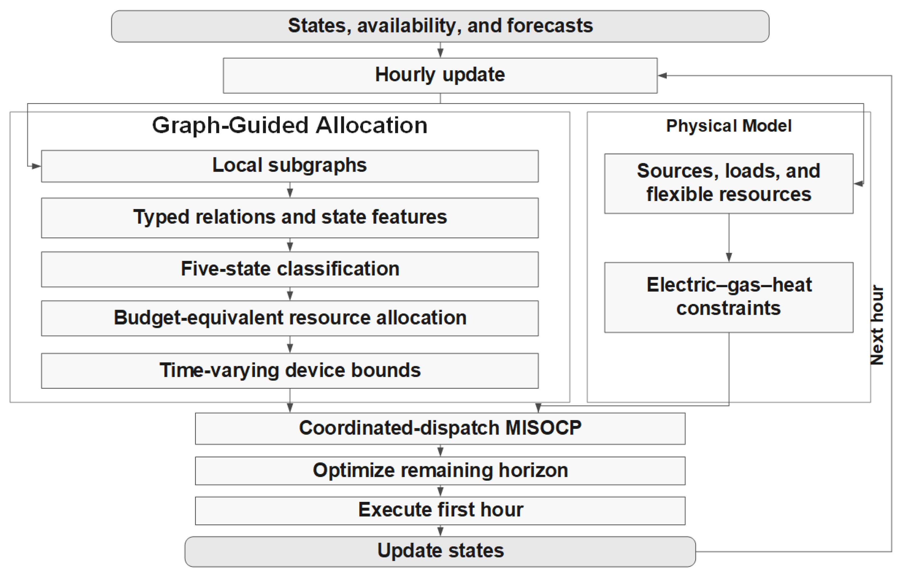
Let the scheduling horizon be $\mathcal{T}=\{1,2,\dots ,T\}$ with time step $\Delta t$. Renewable-availability and load profiles are forecast inputs, while storage states, device outputs, network flows, and load regulation are optimization variables. Installed capacities, candidate connection locations, and the normal-day electric and gas topologies are exogenous. At the beginning of each operating hour, the executed fixed- and mobile-storage states, mobile-storage connection/transit status, current equipment availability, and remaining-horizon forecasts are used to regenerate the classification and callable-capacity factors. The remaining horizon is optimized, only the first-hour decision is committed, and the resulting state initializes the next update. The method therefore performs dynamic operational resource allocation and coordinated dispatch; it does not determine siting, expansion, or installed capacity. The overall workflow of the proposed method is illustrated in Figure 1.

Abbreviations Section summarizes the principal abbreviations and notation. Additional device-specific symbols are defined beside their equations.

2.2. Distributed Renewable Energy and Load Modeling

The optimization receives available PV and wind profiles directly. It does not reconstruct them from irradiance, temperature, or wind speed. For renewable unit g, actual production and curtailment satisfy

$$P_{g,t}^{ren}+P_{g,t}^{curt}={\overline{P}}_{g,t}^{ren},P_{g,t}^{ren},P_{g,t}^{curt}\ge 0.$$

(1)

The load side is divided into fixed, shiftable, flexible-shedding, and critical components. For electric node i, the baseline load is

$$P_{i,t}^0=P_{i,t}^{fix}+P_{i,t}^{tr,0}+P_{i,t}^{fl,0}+P_{i,t}^{cr,0},$$

(2)

where the superscripts denote fixed, transferable, flexible, and critical load, respectively. With transferred-in and transferred-out quantities $\Delta P_{i,t}^{tr,+}$ and $\Delta P_{i,t}^{tr,-}$, the realized transferable demand is

$$P_{i,t}^{tr}=P_{i,t}^{tr,0}+\Delta P_{i,t}^{tr,+}-\Delta P_{i,t}^{tr,-}.$$

(3)

Load shifting preserves total energy and respects period-specific bounds:

$$\left\{\begin{array}{c}\sum _{t\in \mathcal{T}}\Delta P_{i,t}^{tr,+}=\sum _{t\in \mathcal{T}}\Delta P_{i,t}^{tr,-},\hfill \\ 0\le \Delta P_{i,t}^{tr,+}\le {\overline{\Delta P}}_{i,t}^{tr,+},\hfill \\ 0\le \Delta P_{i,t}^{tr,-}\le {\overline{\Delta P}}_{i,t}^{tr,-}.\hfill \end{array}\right.$$

(4)

Let $L{S}_{i,t}^{fl}$ and $L{S}_{i,t}^{cr}$ denote flexible and critical energy not supplied (ENS). Their operating bounds are

$$\left\{\begin{array}{c}0\le L{S}_{i,t}^{fl}\le P_{i,t}^{fl,0},\sum _{t\in \mathcal{T}}L{S}_{i,t}^{fl}\Delta t\le E_i^{fl,max},\hfill \\ 0\le L{S}_{i,t}^{cr}\le P_{i,t}^{cr,0}.\hfill \end{array}\right.$$

(5)

Critical ENS is retained only as a high-penalty feasibility safeguard. It is zero within numerical tolerance in all reported normal-day runs. The realized electric load is

$$P_{i,t}^L=P_{i,t}^{fix}+P_{i,t}^{tr}+P_{i,t}^{fl,0}-L{S}_{i,t}^{fl}+P_{i,t}^{cr,0}-L{S}_{i,t}^{cr}.$$

(6)

The corresponding demand–response cost is

$$C^{DR}=\sum _{t\in \mathcal{T}}\sum _i\left[c_i^{tr}\left(\Delta P_{i,t}^{tr,+}+\Delta P_{i,t}^{tr,-}\right)+c_i^{fl}L{S}_{i,t}^{fl}+c_i^{cr}L{S}_{i,t}^{cr}\right]\Delta t.$$

(7)

The same shift-conservation and flexible/critical ENS structure is used for gas and heat demand where those components are enabled. This formulation changes the temporal distribution of demand before invoking physical shedding; it does not create demand reduction without an explicit ENS variable and penalty.

2.3. Energy Storage, P2G, and Gas Storage Modeling

Fixed electrical storage transfers energy across periods. Let $P_{b,t}^{ch}$ and $P_{b,t}^{dis}$ be charging and discharging power, $E_{b,t}$ stored energy, and $u_{b,t}^{ch}$ and $u_{b,t}^{dis}$ binary operating states. The operating constraints are:

$$\left\{\begin{array}{c}0\le P_{b,t}^{ch}\le u_{b,t}^{ch}{\overline{P}}_b^{ch},\hfill \\ 0\le P_{b,t}^{dis}\le u_{b,t}^{dis}{\overline{P}}_b^{dis},\hfill \\ u_{b,t}^{ch}+u_{b,t}^{dis}\le 1,\hfill \\ E_{b,t}=(1-{\delta }_b^{es})E_{b,t-1}+{\eta }_b^{ch}{P}_{b,t}^{ch}\Delta t-{\displaystyle \frac{P_{b,t}^{dis}\Delta t}{{\eta }_b^{dis}}},\hfill \\ {\underline{E}}_b\le E_{b,t}\le {\overline{E}}_b.\hfill \end{array}\right.$$

(8)

A strict cyclic terminal condition may be written as

$$E_{b,T}=E_{b,0},$$

(9)

while the implemented model uses a terminal band,

$${\underline{E}}_b^{end}\le E_{b,T}\le {\overline{E}}_b^{end},$$

(10)

which prevents artificial end-of-day depletion without forcing a single terminal value.

Gas storage follows an analogous inventory model. With injection $G_{s,t}^{in}$, withdrawal $G_{s,t}^{out}$, inventory $S_{s,t}$, and binary operating states,

$$\left\{\begin{array}{c}0\le G_{s,t}^{in}\le u_{s,t}^{in}{\overline{G}}_s^{in},\hfill \\ 0\le G_{s,t}^{out}\le u_{s,t}^{out}{\overline{G}}_s^{out},\hfill \\ u_{s,t}^{in}+u_{s,t}^{out}\le 1,\hfill \\ S_{s,t}=(1-{\delta }_s^g)S_{s,t-1}+{\eta }_s^{in}{G}_{s,t}^{in}\Delta t-{\displaystyle \frac{G_{s,t}^{out}\Delta t}{{\eta }_s^{out}}},\hfill \\ {\underline{S}}_s\le S_{s,t}\le {\overline{S}}_s,{\underline{S}}_s^{end}\le S_{s,T}\le {\overline{S}}_s^{end}.\hfill \end{array}\right.$$

(11)

P2G converts electricity into synthetic gas. For unit k,

$$S_{k,t}^{p2g}={\alpha }_k^{p2g}{P}_{k,t}^{p2g},$$

(12)

where ${\alpha }_k^{p2g}$ incorporates conversion efficiency and the gas heating-value convention used by the implementation. Its electrical input is bounded by

$$0\le P_{k,t}^{p2g}\le {\overline{P}}_k^{p2g}.$$

(13)

These constraints define the finite capacities and terminal requirements of fixed storage, gas storage, and P2G.

2.4. CHP Subsystem Modeling

The CHP subsystem connects electric, gas, and heat balances through gas turbines and boilers. For gas turbine u, gas consumption and useful heat are linear in electric output:

$$G_{u,t}^{gt}={\alpha }_u^{gt}{P}_{u,t}^{gt},H_{u,t}^{gt}=h_u^{gt}{P}_{u,t}^{gt}.$$

(14)

Gas- and electric-boiler heat production are

$$H_{g,t}^{gb}={\eta }_g^{gb}{\gamma }^g{G}_{g,t}^{gb},H_{e,t}^{eb}={\eta }_e^{eb}{P}_{e,t}^{eb}.$$

(15)

At a coupled station, the electric balance is

$$P_{i,t}^{PCC}+P_{i,t}^{PV}+P_{i,t}^{WT}+P_{i,t}^{GT}+P_{i,t}^{BT,dis}=L_{i,t}^E+P_{i,t}^{BT,ch}+P_{i,t}^{EB}+P_{i,t}^{P2G},$$

(16)

and the gas balance is

$$V_{i,t}^{NGS}+V_{i,t}^{P2G}+V_{i,t}^{GS,dis}=V_{i,t}^{GT}+V_{i,t}^{GB}+V_{i,t}^{GS,ch}+L_{i,t}^G.$$

(17)

Heat is balanced locally:

$$H_{i,t}^{GT}+H_{i,t}^{GB}+H_{i,t}^{EB}=L_{i,t}^H.$$

(18)

No heat-network transport, temperature, or loss dynamics are solved. Any aggregate heat loss is included in the heat-demand input. Gas-turbine ramping satisfies

$$-R_u^{GT,d}\le P_{u,t}^{GT}-P_{u,t-1}^{GT}\le R_u^{GT,u},$$

(19)

and conversion devices remain within their capacities:

$$0\le P_{u,t}^{GT}\le {\overline{P}}_u^{GT},0\le H_{g,t}^{GB}\le {\overline{H}}_g^{GB},0\le H_{e,t}^{EB}\le {\overline{H}}_e^{EB}.$$

(20)

Thus, CHP participates as a constrained conversion agent rather than an unlimited source. The model contains no cooling subsystem.

2.5. Mobile Energy Storage and Soft Open Point (SOP) Modeling

Mobile energy storage combines storage operation with relocation among candidate buses. Let $z_{m,i,t}$ indicate that unit m is connected at candidate bus i, let $I_{m,t}^{tr}$ indicate transit, and let $a_{m,i,j,t}$ indicate a departure from i to j. Each unit is either connected at one candidate or in transit:

$$\sum _{i\in {\mathsf{\Omega }}_B^M}{z}_{m,i,t}+I_{m,t}^{tr}=1,z_{m,i,t},I_{m,t}^{tr}\in \{0,1\}.$$

(21)

Let ${\tau }_{ij,t}$ be the integer travel time for a departure in period t. A departure can occur only from the current location, and the location recursion includes arrivals after the required travel time:

$$\left\{\begin{array}{c}\sum _{j\ne i}{a}_{m,i,j,t}\le z_{m,i,t},a_{m,i,i,t}=0,\hfill \\ z_{m,j,t}=z_{m,j,t-1}-\sum _{h\ne j}{a}_{m,j,h,t-1}+\sum _{i\ne j}\sum _{s:s+{\tau }_{ij,s}=t}{a}_{m,i,j,s}.\hfill \end{array}\right.$$

(22)

This time-expanded recursion separates connected and in-transit periods. Charging, discharging, and reactive support are possible only at the connected bus:

$$\left\{\begin{array}{c}0\le P_{m,i,t}^{M,ch}\le z_{m,i,t}{\overline{P}}_m^{M,ch},\hfill \\ 0\le P_{m,i,t}^{M,dis}\le z_{m,i,t}{\overline{P}}_m^{M,dis},\hfill \\ \sum _i{P}_{m,i,t}^{M,ch}\le u_{m,t}^{M,ch}{\overline{P}}_m^{M,ch}(1-I_{m,t}^{tr}),\hfill \\ \sum _i{P}_{m,i,t}^{M,dis}\le u_{m,t}^{M,dis}{\overline{P}}_m^{M,dis}(1-I_{m,t}^{tr}),\hfill \\ u_{m,t}^{M,ch}+u_{m,t}^{M,dis}\le 1.\hfill \end{array}\right.$$

(23)

The mobile-storage energy recursion is:

$$E_{m,t}^M=(1-{\delta }_m^M)E_{m,t-1}^M+{\eta }_m^{M,ch}\sum _i{P}_{m,i,t}^{M,ch}\Delta t-{\displaystyle \frac{{\sum }_i{P}_{m,i,t}^{M,dis}\Delta t}{{\eta }_m^{M,dis}}}.$$

(24)

Energy and terminal bounds are

$$\left\{\begin{array}{c}{\underline{E}}_m^M\le E_{m,t}^M\le {\overline{E}}_m^M,\hfill \\ E_{m,0}^M=E_m^{M,ini},\hfill \\ {\underline{E}}_m^{M,end}\le E_{m,T}^M\le {\overline{E}}_m^{M,end}.\hfill \end{array}\right.$$

(25)

Travel consumes integer time but no battery energy in the present implementation. The equivalent active injection at bus i is

$$P_{i,t}^M=\sum _{m\in {\mathsf{\Omega }}_M}\left(P_{m,i,t}^{M,dis}-P_{m,i,t}^{M,ch}\right).$$

(26)

For a lossless two-terminal SOP connecting buses i and j, the port-balance and converter-capacity constraints are

$$\left\{\begin{array}{c}{P}_{i,t}^{SOP}+P_{j,t}^{SOP}=0,Q_{i,t}^{SOP}+Q_{j,t}^{SOP}=0,\hfill \\ {\left(P_{i,t}^{SOP}\right)}^2+{\left(Q_{i,t}^{SOP}\right)}^2\le {\left({\overline{S}}_i^{SOP}\right)}^2,\hfill \\ {\left(P_{j,t}^{SOP}\right)}^2+{\left(Q_{j,t}^{SOP}\right)}^2\le {\left({\overline{S}}_j^{SOP}\right)}^2.\hfill \end{array}\right.$$

(27)

The loss term is set to $P_{loss,t}^{SOP}=0$. The SOP redistributes power and provides reactive support but does not create generation.

2.6. Electric–Gas–Heat Coupled Network Model

2.6.1. Distribution-Network Model

The radial distribution system uses the branch-flow DistFlow model [21,22]. For branch $i\to j$,

$$\left\{\begin{array}{c}{P}_{ij,t}-r_{ij}{\mathsf{\ell }}_{ij,t}=\sum _{k:j\to k}{P}_{jk,t}+p_{j,t},\hfill \\ Q_{ij,t}-x_{ij}{\mathsf{\ell }}_{ij,t}=\sum _{k:j\to k}{Q}_{jk,t}+q_{j,t},\hfill \\ v_{j,t}=v_{i,t}-2(r_{ij}{P}_{ij,t}+x_{ij}{Q}_{ij,t})+(r_{ij}^2+x_{ij}^2){\mathsf{\ell }}_{ij,t}.\hfill \end{array}\right.$$

(28)

Voltage and current remain within their security bounds:

$${\underline{v}}_i\le v_{i,t}\le {\overline{v}}_i,0\le {\mathsf{\ell }}_{ij,t}\le {\overline{\mathsf{\ell }}}_{ij}.$$

(29)

The quadratic branch relation is relaxed to the second-order cone

$$P_{ij,t}^2+Q_{ij,t}^2\le v_{i,t}{\mathsf{\ell }}_{ij,t}.$$

(30)

Together, these constraints enforce voltage and line-capacity limits within the common conic model.

2.6.2. Natural Gas Network Model

For physical interpretation, steady-state flow in pipeline $a=(m,n)$ follows the pressure-driven form [23]

$$F_{a,t}=\mathrm{sgn}(p_{m,t},p_{n,t})C_a\sqrt{|p_{m,t}^2-p_{n,t}^2|},$$

(31)

where

$$\mathrm{sgn}(p_{m,t},p_{n,t})=\left\{\begin{array}{cc}1,\hfill & p_{m,t}\ge p_{n,t},\hfill \\ -1,\hfill & p_{m,t}<p_{n,t}.\hfill \end{array}\right.$$

(32)

At gas node i, inflow and injection equal outflow and demand:

$$\sum _{m\in {\mathsf{\Omega }}_i^{in}}{F}_{mi,t}+G_{i,t}^{main}+S_{i,t}^{p2g}+G_{i,t}^{st,out}=\sum _{n\in {\mathsf{\Omega }}_i^{out}}{F}_{in,t}+G_{i,t}^{gt}+G_{i,t}^{gb}+G_{i,t}^{st,in}+L_{i,t}^G.$$

(33)

Pressure and pipeline flow satisfy

$${\underline{p}}_i\le p_{i,t}\le {\overline{p}}_i,-{\overline{F}}_a\le F_{a,t}\le {\overline{F}}_a.$$

(34)

The optimization does not solve the nonconvex square-root equality directly. With squared pressure ${\mathsf{\Pi }}_{i,t}=p_{i,t}^2$, directional nonnegative flows, and a binary direction variable, it uses

$$F_{a,t}=F_{a,t}^{+}-F_{a,t}^{-},{\mathsf{\Pi }}_{m,t}-{\mathsf{\Pi }}_{n,t}=K_a\left(Y_{a,t}^{+}-Y_{a,t}^{-}\right).$$

(35)

$Y_{a,t}^{+}$ and $Y_{a,t}^{-}$ approximate ${\left(F_{a,t}^{+}\right)}^2$ and ${\left(F_{a,t}^{-}\right)}^2$ using seven-breakpoint SOS2 functions. This is a mixed-integer piecewise-linear gas-flow approximation, not an exact nonconvex Weymouth equality.

2.7. Dynamic Operating-State Classification and Rapid Resource-Capacity Allocation Based on Local Subgraphs

2.7.1. Basis for Local Subgraph Division and Typed Relations

The method is formulated for a general electric network ${\mathcal{G}}_E=(\mathcal{N},\mathcal{E})$. Its nodes are first partitioned into K nonempty connected local subgraphs. At each operational update, the available state and forecast information classify these subgraphs and determine their callable resource capacity. With $\mathcal{Z}=\{1,\dots ,K\}$ denoting the subgraph index set, the partition satisfies

$$\mathcal{N}=\bigcup _{z\in \mathcal{Z}}{\mathcal{N}}_z,{\mathcal{N}}_z\ne ⌀,{\mathcal{N}}_z\cap {\mathcal{N}}_{z^{\prime }}=⌀(z\ne z^{\prime }),z,z^{\prime }\in \mathcal{Z}.$$

(36)

The node-to-zone mapping $z\left(i\right)\in \mathcal{Z}$ assigns each node to one and only one local subgraph. At the zone level, the source–load association graph is

$${\mathcal{G}}_Z=\left(\mathcal{Z},{\left\{{\mathbf{A}}^{\left(r\right)}\right\}}_{r=1}^5\right),$$

(37)

where the five zero-diagonal matrices represent electrical adjacency, renewable–load complementarity, storage support, multi-energy coupling, and SOP transfer. Cross-zone electrical capacity defines

$${\widehat{A}}_{z{z}^{\prime }}^{\left(1\right)}=\sum _{\mathsf{\ell }:z\left(f_{\mathsf{\ell }}\right)=z,z\left(t_{\mathsf{\ell }}\right)=z^{\prime }}{\overline{S}}_{\mathsf{\ell }},A_{z{z}^{\prime }}^{\left(1\right)}={\displaystyle \frac{{\widehat{A}}_{z{z}^{\prime }}^{\left(1\right)}+{\widehat{A}}_{z^{\prime }z}^{\left(1\right)}}{{\max }_{a,b}{\widehat{A}}_{ab}^{\left(1\right)}+\epsilon }}.$$

(38)

For nonnegative zone vectors $\mathbf{u}$ and $\mathbf{v}$, the remaining source–sink relations use

$$\mathcal{R}(\mathbf{u},\mathbf{v})=\mathrm{norm}\left({\displaystyle \frac{\mathbf{u}}{{\max }_z{u}_z+\epsilon }}{\displaystyle \frac{{\mathbf{v}}^{\mathsf{T}}}{{\max }_z{v}_z+\epsilon }}+{\displaystyle \frac{\mathbf{v}}{{\max }_z{v}_z+\epsilon }}{\displaystyle \frac{{\mathbf{u}}^{\mathsf{T}}}{{\max }_z{u}_z+\epsilon }}\right),$$

(39)

where $\mathrm{norm}(·)$ zeros the diagonal and divides by the largest entry plus $\epsilon$. Thus,

$$\begin{array}{cc}\hfill {\mathbf{A}}^{\left(2\right)}& =\mathcal{R}(\overline{\mathbf{R}},\overline{\mathbf{L}}),\hfill \end{array}$$

(40)

$$\begin{array}{cc}\hfill {\mathbf{A}}^{\left(3\right)}& =\mathcal{R}({\mathbf{C}}^{sto},{\overline{\mathbf{L}}}^{cri}),\hfill \end{array}$$

(41)

$$\begin{array}{cc}\hfill {\mathbf{A}}^{\left(4\right)}& =\mathcal{R}({\mathbf{C}}^{conv},\overline{\mathbf{L}+\mathbf{R}}),\hfill \end{array}$$

(42)

and ${\mathbf{A}}^{\left(5\right)}$ is built from installed cross-zone SOP ratings.

2.7.2. Five-State Classification

Let $L_{z,t}$ and $R_{z,t}$ be forecast load and available wind-plus-PV generation in zone z. Let $C_z^{sup}$ denote ready storage discharge plus gas-turbine capacity, and let $C_z^{conv}$ denote P2G plus gas-turbine capacity. Storage readiness is evaluated from the state entering the current update; mobile-storage support is assigned only to its current connected zone and is zero in transit. The first four features quantify renewable surplus, critical stress, conversion coupling, and local support shortage, while the fifth measures inter-area transfer need:

$$\begin{array}{cc}{x}_{z,t,1}^{raw}\hfill & =\max (R_{z,t}-L_{z,t},0),\hfill \end{array}$$

(43)

$$\begin{array}{cc}{x}_{z,t,2}^{raw}\hfill & =L_{z,t}^{cri},\hfill \end{array}$$

(44)

$$\begin{array}{cc}{x}_{z,t,3}^{raw}\hfill & ={\displaystyle \frac{C_z^{conv}}{L_{z,t}+C_z^{conv}+\epsilon }},\hfill \end{array}$$

(45)

$$\begin{array}{cc}{x}_{z,t,4}^{raw}\hfill & =\max (L_{z,t}-R_{z,t}-C_z^{sup},0),\hfill \end{array}$$

(46)

$$\begin{array}{cc}{x}_{z,t,5}^{raw}\hfill & =\left|D_{z,t}-{\displaystyle \frac{1}{\left|\mathcal{Z}\right|}}\sum _{j\in \mathcal{Z}}{D}_{j,t}\right|,D_{z,t}=L_{z,t}-R_{z,t}-C_z^{sup}.\hfill \end{array}$$

(47)

Each feature is normalized over the active zone–time set ${\mathcal{T}}_k$ of update k:

$$x_{z,t,f}={\displaystyle \frac{x_{z,t,f}^{raw}-{\min }_{j,\tau }{x}_{j,\tau ,f}^{raw}}{{\max }_{j,\tau }{x}_{j,\tau ,f}^{raw}-{\min }_{j,\tau }{x}_{j,\tau ,f}^{raw}+\epsilon }}.$$

(48)

The safeguard $\epsilon ={10}^{-9}$ maps a constant feature to zero. In a single-shot run, ${\mathcal{T}}_k$ is the complete scheduling horizon. In rolling operation, it contains the current hour and the remaining forecast horizon; realized future values are not used. With typed-relation selection $\tau =(2,3,4,3,5)$,

$${\mathbf{W}}^{\left(f\right)}={\mathrm{rowsum}}^{-1}\left({\mathbf{A}}^{\left(1\right)}+{\mathbf{A}}^{\left({\tau }_f\right)}+\mathbf{I}\right),{\tilde{\mathbf{x}}}_{t,f}=0.65{\mathbf{x}}_{t,f}+0.35{\mathbf{W}}^{\left(f\right)}{\mathbf{x}}_{t,f}.$$

(49)

Topology-only allocation retains only ${\mathbf{A}}^{\left(1\right)}$; graph-guided allocation retains all five matrices. For the five states renewable absorption, critical support, multi-energy coupling, terminal supply, and inter-area support,

$$s_{z,t,q}={\displaystyle \sum _{f=1}^5}{\mathsf{\Xi }}_{qf}{\tilde{x}}_{z,t,f},q_{z,t}^{★}=\arg \underset{q\in \{1,\dots ,5\}}{\max }{s}_{z,t,q}.$$

(50)

All state and resource weights are fixed before the reported dispatch runs and are listed in

Table 2. Fixed classification and resource-allocation weights.

State	Surplus	Critical	Coupling	Support	Transfer
Renewable absorption	0.55	0.05	0.20	0.05	0.15
Critical support	0.05	0.55	0.10	0.20	0.10
Multi-energy coupling	0.15	0.10	0.55	0.10	0.10
Terminal supply	0.05	0.20	0.10	0.50	0.15
Inter-area support	0.10	0.15	0.05	0.20	0.50
Resource	RA	CS	MC	TS	IA
BESS charge	0.55	0.05	0.25	0.05	0.10
BESS discharge	0.05	0.45	0.05	0.30	0.15
P2G	0.45	0.05	0.45	0.02	0.03
GT	0.02	0.35	0.25	0.30	0.08

Factor targets/amplitudes: BESS charge 0.92/0.06; BESS discharge 0.92/0.06; P2G 0.86/0.08; GT 0.94/0.05. RA, CS, MC, TS, and IA denote the five states in table order.

.

2.7.3. Budget-Equivalent Callable-Capacity Allocation

For resource channel $r\in${BESS charge, BESS discharge, P2G, GT}, zone priority is

$$p_{r,z,t}={\displaystyle \sum _{q=1}^5}{\eta }_{rq}{s}_{z,t,q}.$$

(51)

For device d in zone $z\left(d\right)$ with rating $C_{r,d}$, the capacity-weighted center is

$${\overline{p}}_r={\displaystyle \frac{{\sum }_d{\sum }_t{C}_{r,d}{p}_{r,z\left(d\right),t}}{T{\sum }_d{C}_{r,d}}},$$

(52)

and the callable factor is

$${\varphi }_{r,d,t}={\overline{\varphi }}_r+a_r\left(p_{r,z\left(d\right),t}-{\overline{p}}_r\right).$$

(53)

The chosen targets and amplitudes keep $0\le {\varphi }_{r,d,t}\le 1$. Capacity-weighted centering gives

$$\sum _d\sum _t{C}_{r,d}{\varphi }_{r,d,t}=T{\overline{\varphi }}_r\sum _d{C}_{r,d}.$$

(54)

Thus, static, topology-only, and graph-guided allocations have the same aggregate callable-capacity budget. The factors enter the physical optimization directly:

$$\begin{array}{cccc}\hfill 0\le P_{b,t}^{ch}& \le {\varphi }_{ch,b,t}{\overline{P}}_b^{ch}{u}_{b,t}^{ch},\hspace{1em}\hfill & \hfill \hspace{1em}0\le P_{b,t}^{dis}& \le {\varphi }_{dis,b,t}{\overline{P}}_b^{dis}{u}_{b,t}^{dis},\hfill \end{array}$$

(55)

$$\begin{array}{cccc}\hfill 0\le P_{k,t}^{p2g}& \le {\varphi }_{p2g,k,t}{\overline{P}}_k^{p2g},\hspace{1em}\hfill & \hfill \hspace{1em}0\le P_{u,t}^{gt}& \le {\varphi }_{gt,u,t}{\overline{P}}_u^{gt}.\hfill \end{array}$$

(56)

The unrestricted centralized benchmark sets every factor to one and therefore supplies a lower bound for the restricted allocation cases up to their reported optimality intervals.

For the online implementation, Equation (54) is applied within each active window. After the first-hour variables are committed, fixed-storage energy, mobile-storage energy, connection location, transit status, and device availability are updated as fixed inputs to the next window. Consequently, previous dispatch decisions can change the next classification without creating circular dependence inside the current optimization.

2.8. Objective Function, Problem Class, and Evaluation Design

The full objective comprises the following operating-cost components:

$$\begin{array}{cc}\min J=\sum _{t\in \mathcal{T}}\Delta t[\hfill & c_t^e{P}_t^{grid}+c_t^g{G}_t^{main}+c^{pv}{P}_t^{pv,curt}+c^{wt}{P}_t^{wt,curt}\hfill \end{array}$$

(57)

$$\begin{array}{cc}\hfill & +c^{sh,e}(P_t^{sh,in}+P_t^{sh,out})+w^{e,fl}L{S}_t^{e,fl}+w^{e,cr}L{S}_t^{e,cr}\hfill \end{array}$$

(58)

$$\begin{array}{cc}\hfill & +c^{bess}(P_t^{ch}+P_t^{dis})+c^{mess}(P_t^{ms,ch}+P_t^{ms,dis})+c^{sop}\left|P_t^{sop}\right|\hfill \end{array}$$

(59)

$$\begin{array}{cc}\hfill & +c^{gst}(G_t^{st,in}+G_t^{st,out})+c^{gt}{P}_t^{gt}+c^{p2g}{P}_t^{p2g}+c^{bio}{S}_t^{bio}\hfill \end{array}$$

(60)

$$\begin{array}{cc}\hfill & +c^{sh,g}(G_t^{sh,in}+G_t^{sh,out})+w^{g,fl}L{S}_t^{g,fl}+w^{g,cr}L{S}_t^{g,cr}\hfill \end{array}$$

(61)

$$\begin{array}{cc}\hfill & +c^{sh,h}(H_t^{sh,in}+H_t^{sh,out})+w^{h,fl}L{S}_t^{h,fl}+w^{h,cr}L{S}_t^{h,cr}].\hfill \end{array}$$

(62)

Device and node indices are suppressed in Equation (62) for readability. Optional switching and voltage-deviation terms exist in the common electric objective but have zero coefficients in this study. Carbon and a renewable-utilization target are not objective terms. Renewable utilization and supply rate are evaluation metrics.

The complete model contains continuous dispatch and network variables, binary storage, movement, and gas-direction variables, second-order-cone constraints, and SOS2 gas-flow approximations. It is therefore a mixed-integer second-order cone program (MISOCP), with the graph policy acting through the device bounds of the centralized dispatch formulation.

The primary normal-day cost comparison evaluates equal-budget static allocation, topology-only dynamic allocation, and graph-guided dynamic allocation in one 24 h full-horizon solve per policy. Common forecasts, installed ratings, and physical constraints isolate the effect of the allocation mapping. In rolling operation, the policy is regenerated after each committed hour as described above. Complementary tests remove mobile storage, SOPs, or P2G plus CHP; vary fixed-storage capacity, SOP rating, P2G conversion, ENS penalty, and graph-relation strength; perturb renewable and load forecasts; and impose line, SOP, and upstream gas-capacity contingencies. A centralized MPC benchmark uses a 6 h look-ahead and 1 h commitment.

The model dimensions, numerical settings, and computation times are reported with the results in Section 3.

3. Results

3.1. Test System, Numerical Settings, and Model Scale

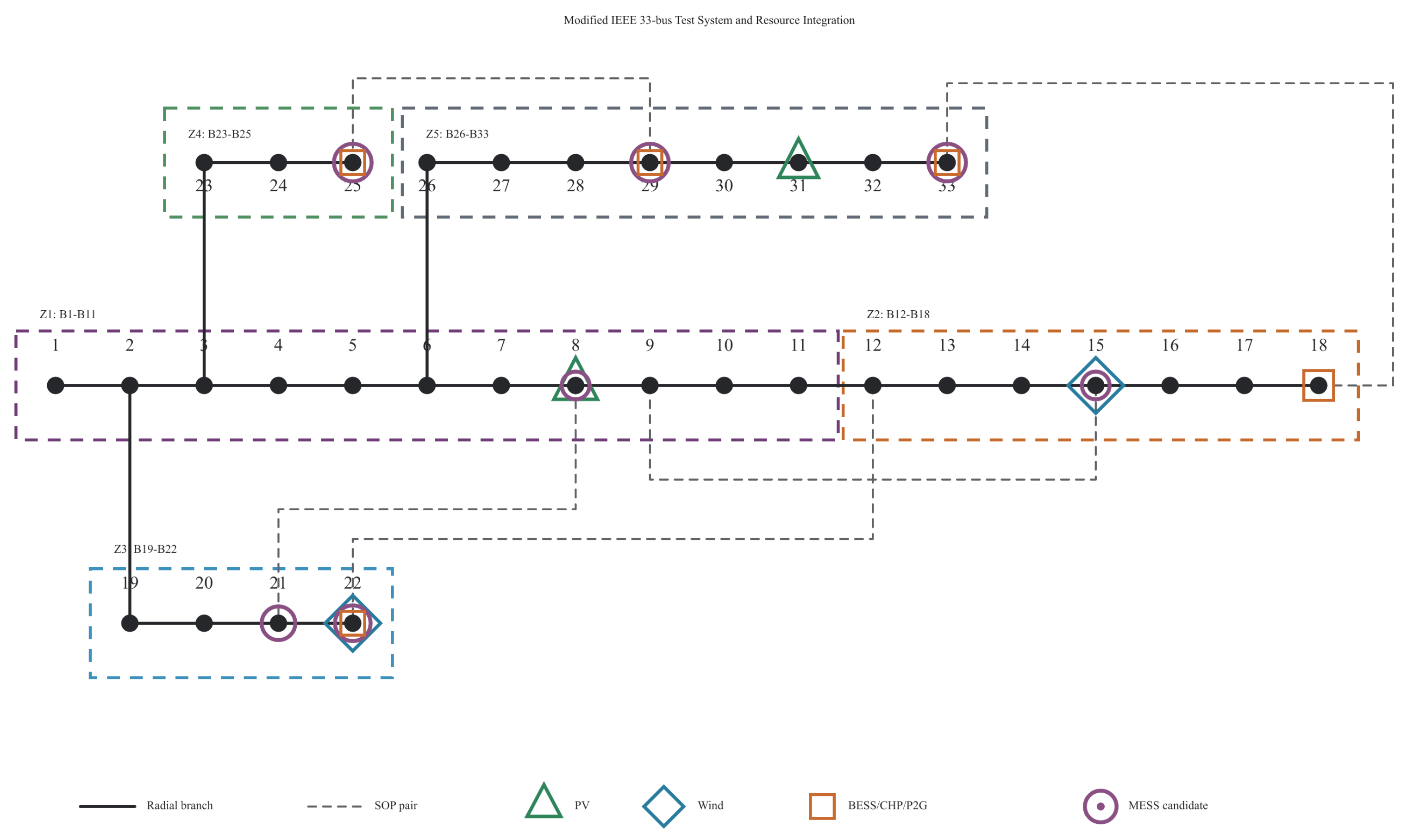
The electric subsystem is based on the radial IEEE 33-bus feeder introduced by Baran and Wu [21]. Its multiple laterals and end-of-feeder voltage constraints make spatial source–load coordination observable while permitting repeated mixed-integer conic studies. The feeder is modified by adding two PV plants (B8 and B31), two wind plants (B15 and B22), and five co-located fixed-storage/CHP/P2G stations (B18, B22, B25, B29, and B33). Two relocatable storage units can connect at B8, B15, B21, B22, B25, B29, or B33. Five SOP pairs connect B8–B21, B9–B15, B12–B22, B18–B33, and B25–B29. The graph layer uses five connected zones: B1–B11, B12–B18, B19–B22, B23–B25, and B26–B33.

The normal operating-day profiles are spatially configured to represent a feeder-end-dominated source–load pattern while preserving the total daily load, renewable energy, and installed ratings. Specifically, 35% of the load originally assigned to B2–B25 is reassigned to B26–B33 and shifted by 1 h; 60% of the renewable profile originally connected at feeder-end buses is reassigned to the existing non-end renewable buses; and 50% of the aggregate fixed-storage and gas-turbine ratings is assigned to the feeder-end station group. These quantities are common input data for all three allocation policies.

Table 3. Main test-system configuration.

Component	Location and Rating	Model Detail
PV	B8 and B31; 0.90 MW each at profile peak	Available profile with explicit curtailment
Wind	B15 (0.80 MW) and B22 (1.00 MW) at profile peak	Available profile with explicit curtailment
Fixed storage	B18/B22/B25/B29/B33; 0.49 MW total; 1.00 MWh total	95% charge/discharge efficiency and terminal bands
CHP and P2G	B18/B22/B25/B29/B33; 0.40 MW GT and 0.20 MW P2G total	Electric–gas–heat linear conversions
Mobile storage	2 units; 1.50 MW, 3.20 MWh total; seven candidate buses	Relocatable, integer travel time, unavailable in transit
SOP	5 pairs; 1.88 MW aggregate active rating	Lossless bidirectional active/reactive exchange
Networks	33-bus electric, 8-node gas, 5 local heat nodes	SOC DistFlow, SOS2 gas flow, local heat balance
Horizon	24 one-hour periods	Day-ahead deterministic base case

gives the principal ratings and terminal conditions.

Figure 2 shows the modified IEEE 33-bus test system and the five connected zones used by the graph layer. Device locations, mobile-storage candidates, and SOP terminal pairs correspond to the case configuration described above.

The numerical experiments were performed on Windows 11 using an Intel Core i7-12700H processor and up to 12 parallel threads. The three normal-day allocation cases used a 2% target optimality gap and a 300 s limit. The ablation, sensitivity, and contingency cases used a 0.5% target gap and the same time limit. Each 6 h MPC window used a 1% target gap and a 120 s limit, while the deterministic and Monte Carlo forecast-error cases used a 1% target gap, a 600 s limit, and one thread. Randomized runs used a fixed seed of 20260715. The achieved gaps are reported with the corresponding results.

The original monetary coefficients were specified in USD. All monetary quantities in this paper are reported in CNY using the fixed conversion rate 1 USD = 7.20 CNY. Because the coefficients are scaled uniformly, the dispatch decisions, optimality gaps, and percentage comparisons are unchanged.

Each full-horizon normal-day model contains 64,669 linear rows, 36,934 columns, 3526 binary variables, 1776 quadratic constraints, and 384 SOS constraints. Optimization time measures the numerical solution phase, while wall time also includes model construction, solution extraction, and file handling. The graph-guided objective reconstruction error is $4.59\times {10}^{-11}$ CNY, the DistFlow SOC slack ranges from $1.12\times {10}^{-10}$ to $2.08\times {10}^{-7}$, and no fixed or mobile storage unit charges and discharges simultaneously.

3.2. Operating-State Classification

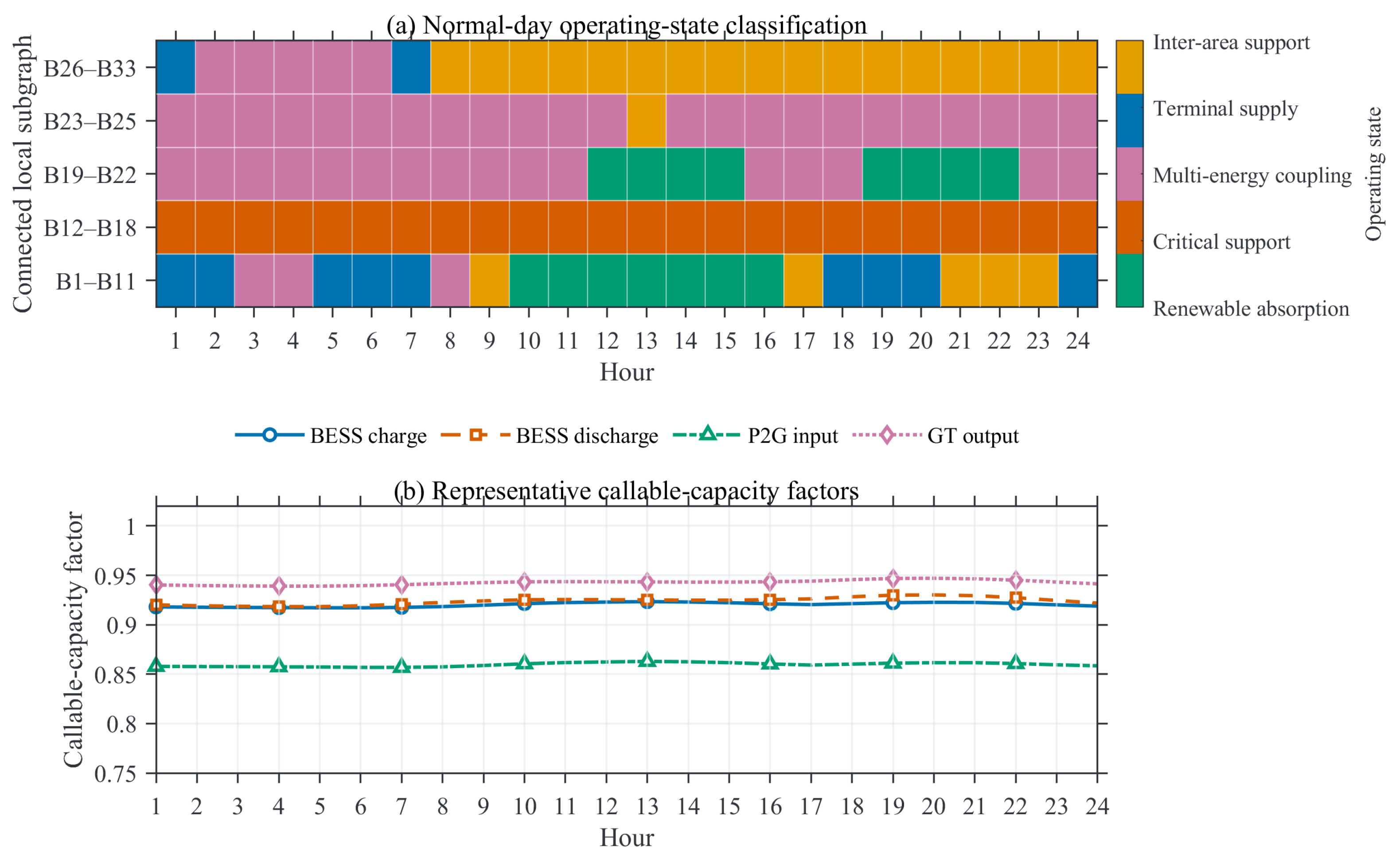
Figure 3 reports the graph-guided state labels and the representative callable-capacity factors of the co-located BESS/P2G/GT station at B33 over the normal operating day. B12–B18 remains in critical-support state throughout the day. B19–B22 alternates between multi-energy coupling and renewable absorption as its renewable profile changes. B26–B33 changes from terminal supply or multi-energy coupling in the early hours to inter-area support from hour 8 onward, reflecting its transferred load and reduced local renewable profile. B1–B11 shows the widest mix of terminal supply, multi-energy coupling, renewable absorption, and inter-area support.

For the reported full-horizon comparison, all labels and factors are generated before the MISOCP solve from the common daily profiles and initial operating state. In the operational rolling implementation, the same calculation is repeated after each committed hour using updated fixed/mobile-storage states and connection availability, as described in Section 2.7. The topology-only policy excludes renewable–load, storage-support, coupling, and SOP relation matrices; the static policy retains the same aggregate target factors but does not vary them by device or time.

3.3. Comparison of Allocation Methods

Table 4. Equal-budget comparison for the normal operating day.

Method	Cost (CNY)	Saving (%)	Wall Time (s)	Gap (%)	Supply (%)
Static equal budget	52,294.33	0.5689	133.0	0.5839	100.000000
Topology-only dynamic	52,829.05	1.5753	236.1	1.6038	100.000000
Graph-guided dynamic	51,996.84	0.0000	135.0	0.0340	100.000000

Each policy uses one 24 h full-horizon solve on the same normal-day profiles and installed ratings. Graph saving is the observed reduction of graph-guided cost relative to the listed policy. Supply and renewable utilization are 100% within numerical tolerance.

compares the three equal-budget allocation policies on the same normal operating-day profiles. The operating costs are 52,294.3274 CNY for static allocation, 52,829.0523 CNY for topology-only allocation, and 51,996.8437 CNY for graph-guided allocation. The graph-guided schedule is 0.568864% below static allocation and 1.575286% below topology-only allocation.

The wall times are 133.0, 236.1, and 135.0 s, and the achieved gaps are 0.5839%, 1.6038%, and 0.0340% for static, topology-only, and graph-guided allocation, respectively. All three policies use 100% of the 41.76 MWh available renewable energy and serve 100% of the 70.85 MWh electric demand within numerical tolerance; the topology-only ENS of $5.02\times {10}^{-9}$ MWh is numerical noise. Thus, the distinguishing result is operating cost. The wider optimality intervals of the two baselines are retained when interpreting the feasible-objective differences.

3.4. Dispatch and Network Trajectories

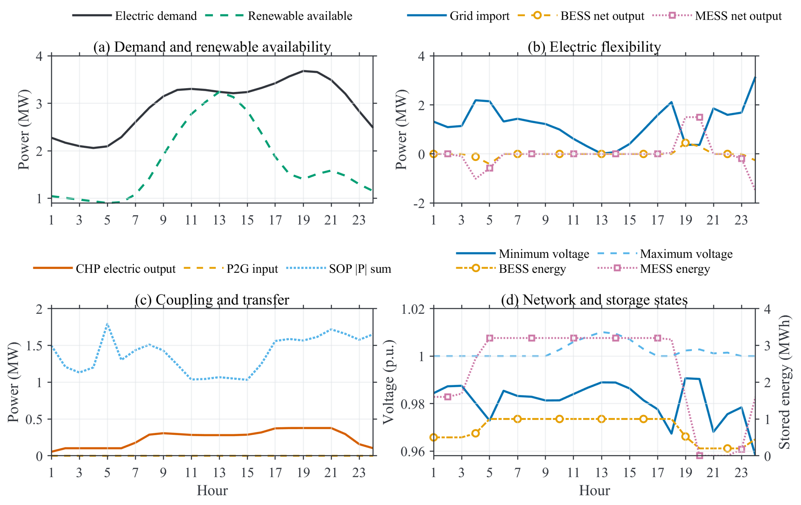
Figure 4 reports the graph-guided normal-day schedule. Renewable availability, electric demand, grid purchase, storage power, CHP output, P2G input, SOP exchange, voltage, and storage states are computed directly from the optimized variables. The schedule purchases 29.2768 MWh of electricity, uses 1.5495 MWh of fixed-storage throughput and 6.4084 MWh of mobile-storage throughput, and produces 5.7969 MWh from the gas turbines. P2G input is $1.57\times {10}^{-7}$ MWh and is treated as inactive on this day.

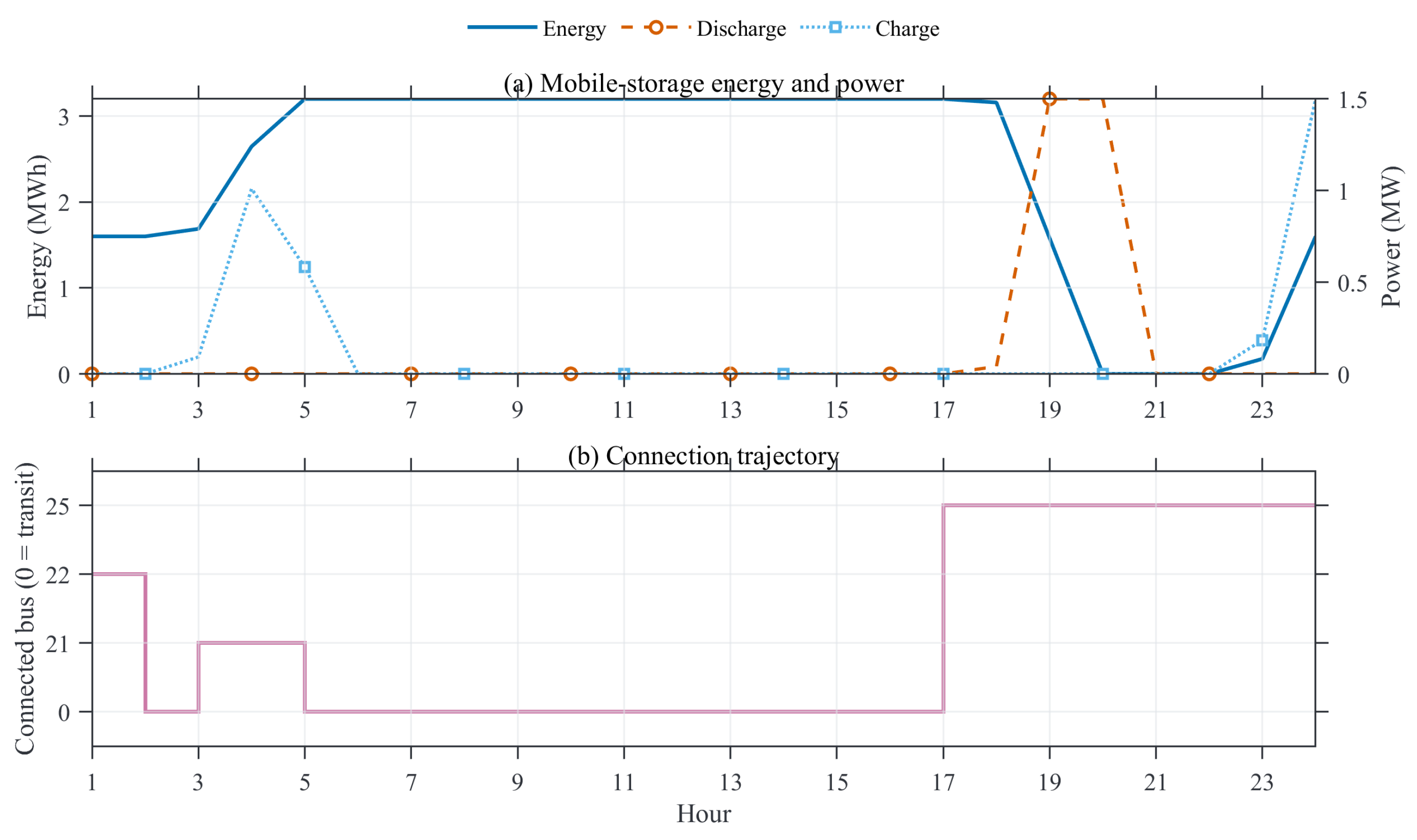
The minimum voltage is 0.9580 p.u., the maximum is 1.0101 p.u., and the maximum line loading is 0.1016 p.u. under the model ratings. Figure 5 shows aggregate mobile-storage energy and power together with the first unit’s connection trajectory. The two units make two relocations in aggregate, remain unavailable for charging and discharging in transit, and finish with 1.60 MWh of aggregate energy. Fixed storage finishes at 0.45 MWh; both storage types satisfy their terminal bands.

3.5. Component Ablation

The component ablations use the same normal operating-day profiles, installed ratings, graph policy, and numerical settings as the graph-guided case in Section 3.3.

Table 5. Component ablation on the normal operating day.

Case	Cost (CNY)	Increase (%)	Flex. ENS (MWh)	MESS (MWh)	SOP $\left|\mathit{P}\right|$ (MWh)	CHP (MWh)
Base graph	51,996.84	0.00	0.00000	6.41	33.15	5.80
No MESS	53,447.45	2.79	0.00000	0.00	32.97	5.80
No SOP	57,686.21	10.94	0.06098	4.94	0.00	7.15
No P2G/CHP	114,727.14	120.64	0.00000	6.41	37.30	0.00

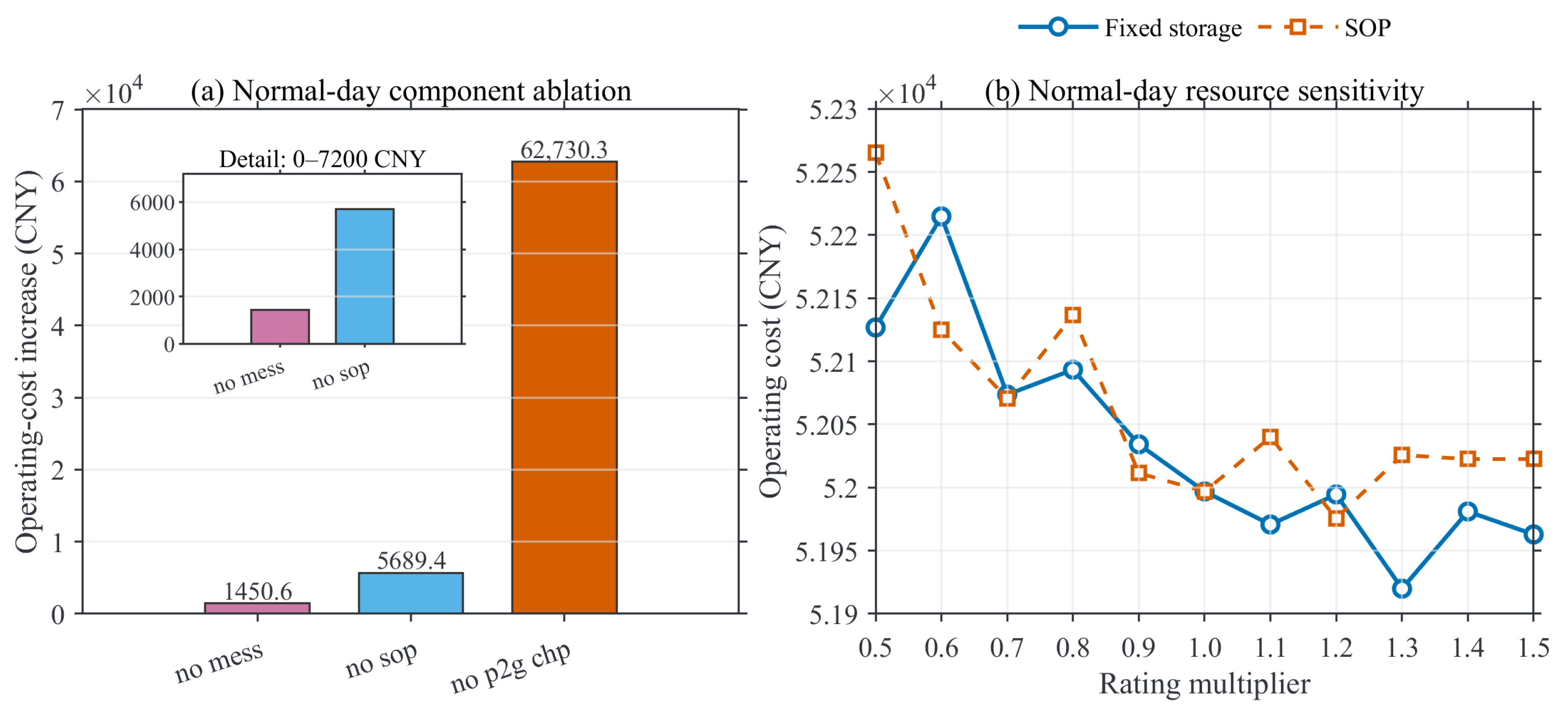
The no-SOP case serves 99.9139% of electric demand and records 0.06098 MWh flexible ENS; critical ENS is zero in all four cases.

isolates three device groups around the 51,996.84 CNY base. Removing mobile storage increases the cost to 53,447.45 CNY, an increase of 1450.61 CNY (2.79%). Removing all SOPs increases the cost to 57,686.21 CNY, an increase of 5689.37 CNY (10.94%), and produces 0.06098 MWh of flexible ENS, corresponding to a 99.9139% power-supply rate. Removing both P2G and CHP increases the cost to 114,727.14 CNY, an increase of 62,730.30 CNY (120.64%). Because P2G input is negligible in the base case, the last increase is attributable primarily to the loss of CHP electric and heat coupling.

These ablations quantify device-layer contributions within the graph-guided schedule and complement the allocation-method comparison. Mobile storage and CHP reduce operating cost, while SOP removal also causes flexible load shedding, demonstrating the operational value of feeder-to-feeder transfer in the tested spatial distribution.

3.6. Parameter Sensitivity

The normal-day sensitivity suite varies fixed-storage capacity and SOP rating from 0.5 to 1.5 in increments of 0.1; Figure 6 shows all points, while

Table 6. Parameter sensitivity on the normal operating day.

Parameter	Multiplier	Cost (CNY)	Grid Purchase (MWh)	Gap (%)
Fixed storage	0.5	52,126.75	29.250	0.0262
Fixed storage	1.0	51,996.84	29.277	0.0340
Fixed storage	1.5	51,962.79	29.404	0.2202
SOP rating	0.5	52,265.04	29.611	0.1646
SOP rating	1.0	51,996.84	29.277	0.0340
SOP rating	1.5	52,022.50	29.301	0.4190
P2G conversion	0.8	52,042.11	29.360	0.1072
P2G conversion	1.0	51,996.84	29.277	0.0340
P2G conversion	1.2	51,996.84	29.277	0.2726
Graph relation	0.8	52,022.32	29.270	0.0824
Graph relation	1.0	51,996.84	29.277	0.0340
Graph relation	1.2	52,061.76	29.504	0.1384

Multiplier-1 rows use the normal-day graph solution; every other row is independently optimized under the same source–load profiles and installed ratings.

retains representative 0.5, 1.0, and 1.5 anchors together with the other parameters. Reducing fixed-storage capacity to 0.5 times its base value increases the incumbent cost to 52,126.75 CNY, 129.90 CNY (0.25%) above the base. Increasing it to 1.5 times gives 51,962.79 CNY, 34.05 CNY (0.07%) below the base. The 0.5-times lower bound (52,113.10 CNY) exceeds the base incumbent, while the 1.5-times incumbent is below the base lower bound (51,979.18 CNY), supporting the endpoint trend despite local fluctuations among the intermediate values.

Reducing the SOP rating to 0.5 times raises the incumbent to 52,265.04 CNY, 268.20 CNY (0.52%) above the base, and its lower bound of 52,178.98 CNY remains above the base incumbent. At 1.5 times, the incumbent is 52,022.50 CNY with a 0.4190% gap, so its interval overlaps the base interval and no additional benefit above the installed rating is resolved. The P2G-conversion and graph-relation intervals also overlap the base interval over the tested 0.8–1.2 range, consistent with negligible P2G use and the absence of a monotonic relation-weight response.

3.7. Contingency Stress Tests

Table 7. Contingency stress-test results.

Case	Cost (CNY)	ENS (MWh)	${\mathit{V}}_{\mathit{min}}$	Line Loading	Opt. Time (s)
Normal-day base	51,996.84	0.00	0.9580	0.1016	74.7
Line 5 outage	205,642.04	1.33	0.9500	0.0993	82.4
SOP 18–33 outage	52,395.47	$6.40\times {10}^{-10}$	0.9591	0.1034	119.6
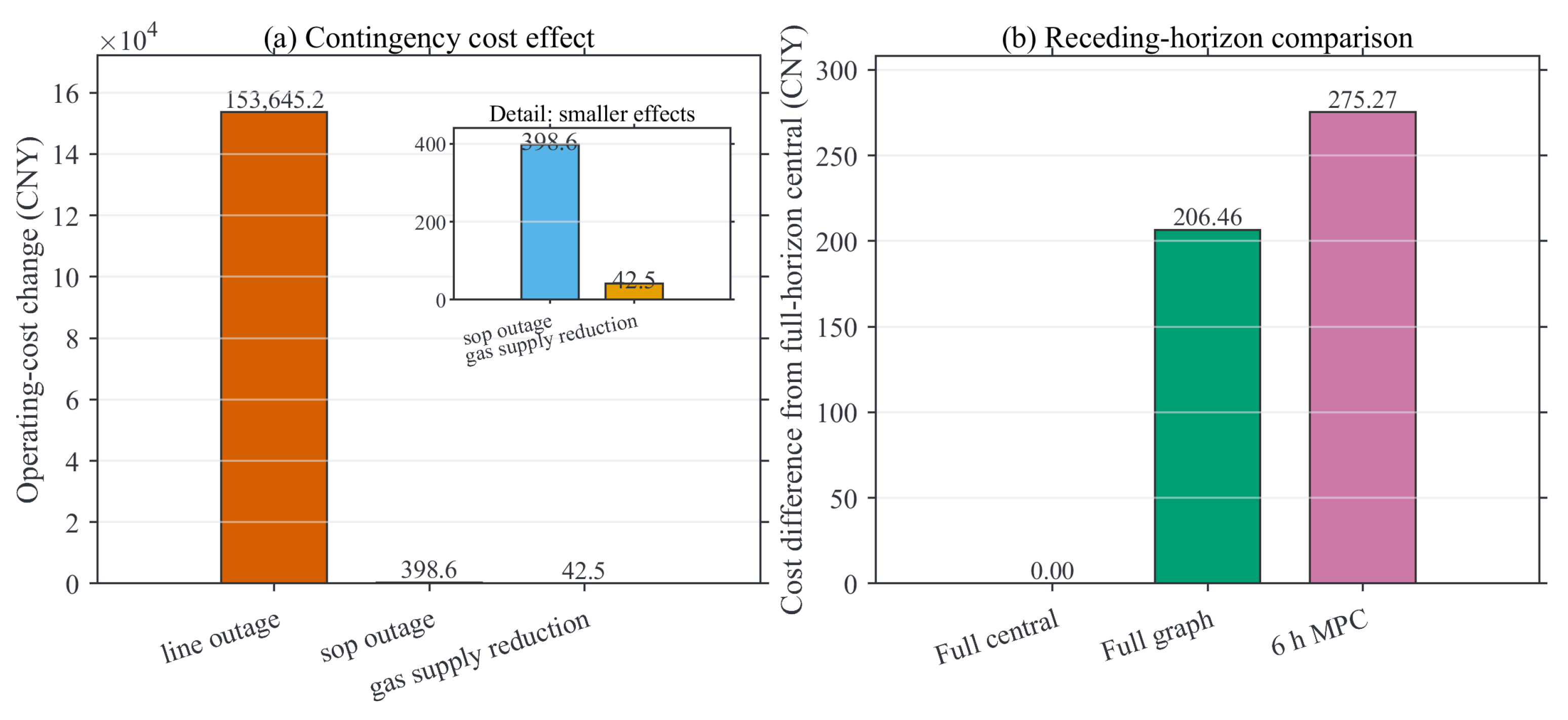
50% gas reduction	52,039.34	0.00	0.9580	0.1016	56.6

reports contingency cases under the fixed normal-day graph policy. A branch-5 outage during hours 18–21 increases the cost from 51,996.84 to 205,642.04 CNY, reduces the minimum voltage to 0.9500 p.u., and produces 1.32632 MWh of total ENS, corresponding to a 98.1279% power-supply rate. Removing the B18–B33 SOP for the full day increases the cost to 52,395.47 CNY; its $6.40\times {10}^{-10}$ MWh ENS is numerical tolerance. A 50% upstream gas-capacity reduction during hours 18–21 increases the cost modestly to 52,039.34 CNY without ENS, indicating that this limit is weakly active on the tested day.

These tests characterize the stress response of the installed system under the graph-guided policy. The line-outage case exposes a severe service-loss condition, whereas the SOP and gas-capacity cases remain close to the normal-day operating point.

3.8. Six-Hour Receding-Horizon Benchmark

Table 8. Full-horizon and receding-horizon comparison.

Method	Cost (CNY)	Opt. Time (s)	Wall Time (s)	Windows
Full-horizon central	51,790.39	211.3	273.0	1
Full-horizon graph	51,996.84	74.7	135.0	1
Central MPC (6 h)	52,065.66	176.8	447.6	24

compares single-shot full-horizon scheduling with centralized MPC using a 6 h look-ahead and a 1 h commitment. The unrestricted central, graph-guided, and MPC costs are 51,790.39, 51,996.84, and 52,065.66 CNY, respectively. MPC is 0.5315% above the unrestricted full-horizon solution and 0.1323% above the graph-guided full-horizon solution.

All 24 MPC windows solve successfully. Aggregate BESS and mobile-storage energy finish at 0.4500 and 1.6000 MWh, respectively, and total ENS is $8.77\times {10}^{-9}$ MWh. Terminal targets are enforced in every receding-horizon window that reaches the end of the scheduling day. Cumulative optimization time is 176.8 s and wall time is 447.6 s. Relative to the graph-guided full-horizon run, these totals are 136.8% and 231.6% higher, respectively. Relative to the unrestricted central run, MPC uses 16.3% less optimization time but 64.0% more wall time because repeated model construction, data transfer, solution extraction, and state updates dominate the daily overhead. Every window completes within the 1 h sampling interval on the stated workstation, supporting the hourly scheduling cadence. Figure 7 summarizes the cost effects of the selected contingencies together with the centralized MPC benchmark.

3.9. Forecast-Error Stress Tests

Table 9. Forecast-error and MPC evaluation.

Case	Cost (CNY)	ENS (MWh)	${\mathit{V}}_{\mathit{min}}$	Opt. Time (s)
Adverse error 5%	56,137.35	0.00	0.9544	53.5
Adverse error 10%	59,909.16	0.00	0.9508	63.2
Adverse error 20%	68,403.74	0.00	0.9500	58.6
Monte Carlo mean	52,142.91	–	0.9584	–
Monte Carlo 95th percentile	53,595.85	–	–	–
Monte Carlo worst case	54,555.62	–	0.9509	–
Central MPC (6 h)	52,065.66	$8.77\times {10}^{-9}$	–	176.8

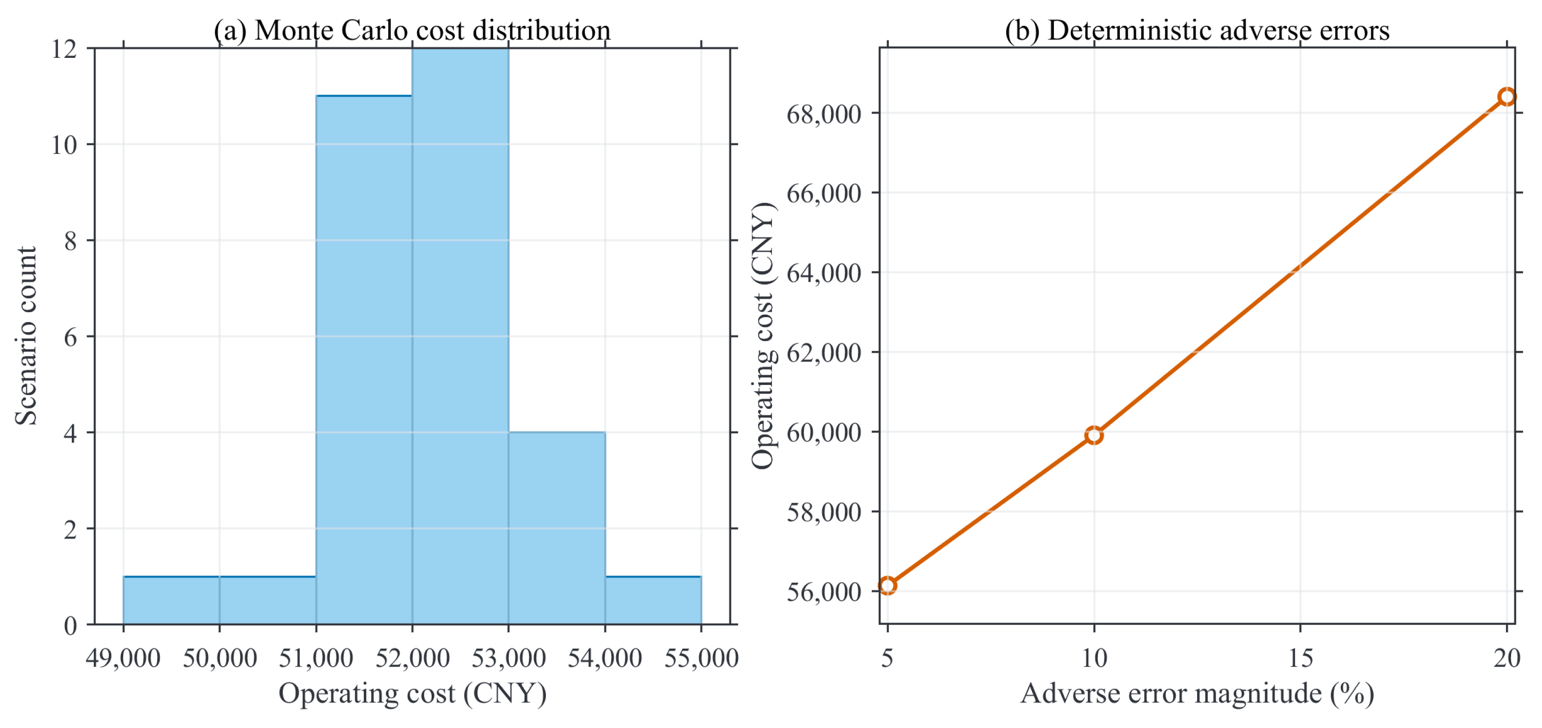
Monte Carlo scenarios use the fixed normal-day graph policy and quantify sensitivity to forecast perturbations.

and Figure 8 summarize the forecast-error tests. Under simultaneous renewable reductions and load increases of 5%, 10%, and 20%, operating cost rises to 56,137.35, 59,909.16, and 68,403.74 CNY, respectively. All three deterministic adverse cases remain feasible without physical renewable curtailment or ENS; the minimum voltage reaches 0.9500 p.u. in the 20% case.

Across the 30 seeded Monte Carlo scenarios, cost ranges from 49,944.63 to 54,555.62 CNY, with a mean of 52,142.91 CNY, a standard deviation of 913.31 CNY, and a 95th percentile of 53,595.85 CNY. Relative to the fixed-policy normal-day base cost of 51,996.84 CNY, the mean is 0.2809% higher and the worst case is 4.9210% higher. The worst minimum voltage is 0.9509 p.u., the maximum line loading is 0.1034 p.u., and the largest achieved optimality gap is 0.5278%.

Optimization time varies across the random instances: its mean is 76.1 s, standard deviation is 29.4 s, 95th percentile is 144.3 s, and maximum is 163.7 s. The maximum remains below the 600 s scenario limit, and the largest achieved gap remains below the 1% target. This spread reflects the instance-dependent nature of mixed-integer search and is therefore reported together with the upper-tail statistics.

The maximum Monte Carlo renewable-curtailment, flexible-ENS, and critical-ENS values are $4.91\times {10}^{-7}$, $2.77\times {10}^{-10}$, and zero MWh, respectively, and are treated as numerical tolerance. These scenarios re-optimize dispatch for perturbed profiles while retaining the normal-day graph policy, thereby quantifying stress sensitivity under a fixed classification policy.

4. Discussion

4.1. What the Association Graph Adds

The association graph augments the physical dispatch model by mapping five typed inter-zone relations to time-varying device bounds at each operating update. Equation (56) embeds this mapping in the dispatch constraints, while Equation (54) gives the graph-guided, static, and topology-only cases the same aggregate callable-capacity budget within each window. Installed ratings and locations remain fixed, so the method allocates operational limits and dispatch rather than planning capacity.

On the normal operating day, graph-guided allocation records the lowest feasible operating cost: 0.5689% below static allocation and 1.5753% below topology-only allocation. Because all three policies achieve 100% supply and renewable utilization, the comparison isolates an economic advantage. The daily profile contains a pronounced spatial separation between feeder-end demand and renewable availability, allowing the typed source–load, storage-support, coupling, and SOP relations to direct the fixed callable budget more effectively than a uniform or topology-only rule. The wider baseline optimality intervals are considered when interpreting these observed cost differences.

4.2. Device Contributions and Physical Interpretation

The normal-day ablations provide complementary device evidence. Removing mobile storage raises the cost by 2.79%, whereas removing SOPs raises the cost by 10.94% and causes 0.06098 MWh of flexible ENS, showing the value of spatially transferable storage and feeder-to-feeder exchange. Removing P2G and CHP has the largest cost effect. Since P2G input is almost zero in the base case; this increase is mainly associated with the loss of CHP electric and heat coupling.

The sensitivity endpoints reinforce this interpretation. Halving fixed-storage capacity or SOP rating increases the cost, and both increases remain separated from the base after accounting for the reported bounds. Increasing fixed storage to 1.5 times yields a lower incumbent than the base lower bound, whereas the 1.5-times SOP interval overlaps the base interval. Thus, added fixed-storage capacity provides a measurable benefit at the endpoint, while additional SOP rating above the installed value has no resolved marginal benefit in this lightly loaded case. Several differences among the 0.1-spaced intermediate points are comparable to their achieved gaps. The negligible P2G response and overlapping relation-strength intervals likewise indicate limited sensitivity over the tested ranges.

The forecast-error tests show a measurable cost spread without physical ENS or renewable curtailment. The Monte Carlo mean is 0.2809% above the normal-day base and the worst sampled cost is 4.9210% above it. The fixed graph policy remains feasible across the sampled perturbations, with dispatch re-optimized for each profile and the classification policy held constant.

4.3. Computational Burden, Timing Variability, and Benchmark Scope

The principal computational burden comes from the centralized mixed-integer dispatch. The 24 h model contains 3526 binary variables, 1776 quadratic constraints, and 384 SOS constraints in addition to its continuous network and device variables. The binary variables represent storage operating modes, mobile-storage connection and movement logic, and gas-flow direction; the quadratic constraints arise primarily from SOC network and apparent-power limits; and the SOS sets implement the gas-flow approximations. These structures create a branch-and-bound problem whose difficulty depends on the active bounds and incumbent search, even when two cases have the same model dimensions.

The graph stage uses five-zone feature vectors and five $5\times 5$ relation matrices to generate the bound parameters, and the same calculation is repeated at every update in rolling operation. The reported full-horizon wall times include graph processing, model construction, data transfer, extraction, and serialization. Because graph-processing time was not recorded separately, the timing results characterize the complete scheduling workflow.

The normal-day static, topology-only, and graph-guided full-horizon wall times are 133.0, 236.1, and 135.0 s, respectively. The graph-guided workflow is faster than topology-only and close to static allocation in this instance. The 6 h centralized MPC requires 447.6 s for 24 windows. Across the 30 forecast-error instances, optimization time has a mean of 76.1 s, a 95th percentile of 144.3 s, and a maximum of 163.7 s. All reported runs complete within the 1 h scheduling interval on the stated workstation.

Graph-guided allocation reaches a 0.0340% optimality gap, compared with 0.5839% for static allocation and 1.6038% for topology-only allocation. The Monte Carlo maximum is 0.5278% under the 1% target. Reporting these values alongside the feasible costs provides the numerical precision needed to interpret small differences among cases.

4.4. Limitations and Generalizability

The numerical study uses one modified IEEE 33-bus system, one normal operating-day spatial distribution, and one workstation. Larger radial and meshed feeders, longer horizons, additional mobile-storage candidates, and more SOPs are needed to characterize computational scaling.

The classification and resource weights are fixed heuristic values, and the relation-strength sensitivity does not show a monotonic response. Multi-day data and independent validation are therefore needed for weight calibration. The Monte Carlo study keeps the normal-day graph policy fixed and re-optimizes dispatch after perturbing the profiles; extending the model to stochastic, robust, or chance-constrained recourse is a further research direction.

Heat is represented by local balance equations without transport temperature and loss dynamics; SOPs are lossless; and mobile-storage travel consumes time without explicit battery-energy consumption. Future work should enrich these physical models, instrument each computational stage, evaluate multi-day rolling operation, and compare centralized and decomposed formulations under common accuracy and stopping criteria.

5. Conclusions

This paper develops a method for dynamic operational resource allocation and coordinated dispatch based on a source–load association graph. At each operating hour, five typed relation matrices, five normalized features, and fixed state/resource weights regenerate callable-capacity factors from the executed storage/location state and remaining-horizon forecasts. These factors enter explicit storage, P2G, and gas-turbine upper bounds. Capacity-weighted centering gives static, topology-only, and graph-guided allocation the same aggregate flexibility budget within each window, while installed capacities and locations remain exogenous.

The electric–gas–heat MISOCP contains SOC DistFlow constraints, SOS2 gas-flow approximations, fixed and mobile storage, CHP, P2G, and SOPs. On the normal operating day, graph-guided dispatch records the lowest feasible operating cost, 51,996.84 CNY, which is 0.5689% below static allocation and 1.5753% below topology-only allocation. All policies serve 100% of demand and use 100% of available renewable energy within numerical tolerance. These results demonstrate the operating-cost advantage of graph-guided allocation for the tested daily spatial distribution.

The ablation and sensitivity studies show that mobile storage, SOPs, and CHP provide complementary flexibility. Removing MESS raises the cost by 2.79%; removing SOPs raises the cost by 10.94% and causes 0.06098 MWh flexible ENS; and removing P2G plus CHP raises the cost by 120.64%, primarily because CHP is lost. The selected line outage causes 1.32632 MWh ENS, while the 30-scenario mean and worst costs are 0.2809% and 4.9210% above the fixed-policy base. The 6 h MPC cost is 0.1323% above the graph-guided full-horizon result. Together with the measured computation times, these findings support hourly operational scheduling on the stated workstation and motivate further validation on larger networks and multi-day rolling scenarios.