Desired-Dynamics-Based Predictive Control (DDPC) for Uncertain Systems: A Unified Framework and Application to Superheated Steam Temperature Control

Abstract

With the increasing prevalence of uncertainties and variability in modern energy systems, model predictive control (MPC) often faces the challenge of predictive model mismatch. This paper proposes a desired-dynamics-based predictive control (DDPC) framework, in which an inner shaping layer is introduced to transform the raw plant into a desired dynamic model for the outer MPC. A unified design methodology is developed, including equivalent-model construction, desired-dynamics selection, and two inner-layer realizations based on desired dynamic equation (DDE)-PID and active disturbance rejection control (ADRC). In this way, the prediction model used by MPC is no longer the original uncertain plant but an explicitly shaped equivalent model determined by inner-layer controller parameters. The proposed method is validated on linear and nonlinear benchmark plants, together with frequency-domain and Monte Carlo robustness analyses. Results show that DDPC improves disturbance-rejection ability and enhances robustness against model mismatch and parameter perturbations. Further evaluation on the superheated steam temperature loop of a high-fidelity 660 MW coal-fired boiler hardware-in-the-loop simulator shows that DDPC reduces the peak-to-peak temperature fluctuation from 22.88 °C to 11.39 °C in the deep peak shaving scenario, corresponding to a 50.2% reduction relative to standard MPC.

1. Introduction

1.1. Control Challenges in Variable-Condition Energy Systems

As the penetration of renewable energy continues to increase, many energy systems are shifting from steady-load operation to fluctuation-driven operation, such as deep peak-shaving coal-fired units [1], wind-energy systems under varying conditions [2], and green-electricity-coupled hydrogen–ammonia processes [3]. In these scenarios, the balance among generation, storage, and load is no longer maintained around a fixed operating point but evolves continuously with renewable power fluctuations, demand variations, and operational constraints. Consequently, control systems are required to maintain accurate regulation, operational safety, and acceptable dynamic performance under nonlinear and load-varying conditions.

A fundamental control difficulty in such systems is that the plant seen by the controller is not dynamically invariant. Load changes may alter process gain, dominant time constants, delay characteristics, heat-storage effects, actuator operating regions, and disturbance propagation paths. As a result, a model identified or calibrated at one operating condition may become inconsistent with the actual plant under another condition [4]. This inconsistency is particularly critical for energy-process control because the controller must simultaneously handle command tracking, disturbance rejection, safety-margin maintenance, coupled-loop coordination, and actuator-movement limitation over a wide operating range. This requirement motivates the development of control methods that can improve robustness against operating-condition variations while retaining the capability to coordinate future behavior, constraints, and control effort.

1.2. Control Methods Under Uncertainty

To address uncertainty and operating-condition variations, existing control methods can be broadly divided into low-model-dependence feedback regulation and model-based predictive optimization. PID-type controllers and active disturbance rejection control (ADRC) are representative feedback-regulation methods. PID control is simple and widely used [5], while ADRC improves robustness by estimating and compensating lumped uncertainty through an extended state observer [6]. These methods do not require a high-fidelity full-order plant model and can provide effective local disturbance rejection. However, when used alone, they do not explicitly solve a finite-horizon constrained optimization problem for future trajectories, input-output constraints, actuator movement, control energy, or multivariable coordination. Their performance also depends on gain tuning, gain scheduling, or observer-bandwidth selection under different operating conditions.

MPC, by contrast, provides finite-horizon prediction, explicit constraint handling, and multivariable optimization [7,8]. Through receding-horizon optimization, it can balance tracking performance, control effort, and operational constraints. However, this advantage depends strongly on the accuracy of the prediction model [4,7]. Under parameter variations, unmodeled dynamics, external disturbances, or changing operating conditions, model mismatch may propagate into the predicted trajectories and distort the resulting optimization decisions [4,9].

Robust MPC incorporates uncertainty descriptions into the optimization problem to provide worst-case guarantees on stability, recursive feasibility, and constraint satisfaction. Representative formulations include min–max MPC [10], tube-based MPC [11,12], and invariant-set-based approaches [13]. Recent studies have extended these methods to LPV systems with interval predictors [12], nonlinear systems with control-contraction-metric-based robust adaptive tubes [14], and tracking MPC with implicit invariant sets [13]. These methods provide rigorous guarantees, but they require reliable uncertainty bounds, tube constructions, or invariant sets. When uncertainty is large, time-varying, or difficult to characterize, the resulting controller may become conservative or computationally demanding.

Stochastic MPC handles uncertainty through probabilistic descriptions, such as chance constraints, scenario sampling, and distributionally robust formulations [15]. Recent examples include conditional scenario-based MPC for correlated parametric uncertainty and additive disturbances [16], distributionally robust MPC for stochastic mixed-traffic flow [17], and Wasserstein-based distributionally robust MPC for smart-grid uncertainties [18]. These methods offer risk-aware control, but their effectiveness depends on the assumed distribution, sample quality, and ambiguity-set design. For nonstationary industrial energy systems, such probabilistic information may be difficult to obtain and maintain.

Adaptive and learning-based MPC reduces prediction mismatch by updating model parameters, model structures, or uncertainty descriptions online [19,20,21]. This can reduce conservatism when sufficient data and identifiable model structures are available. However, adaptive MPC usually requires additional mechanisms for recursive feasibility, closed-loop stability, and safe adaptation. In wide-range industrial operation, these requirements become restrictive because operating regions change continuously, key variables may be inaccessible, and multivariable coupling models are costly to identify and update.

Observer-assisted methods introduce disturbance observers, extended state observers, sliding-mode observers, or offset-free augmentation into MPC. Disturbance-observer-based MPC and sliding-mode-observer-based robust MPC estimate disturbances and compensate for their effects during predictive optimization [22,23]. Event-triggered disturbance-observer-based MPC further reduces computational and communication burden [24]. Modified active disturbance rejection predictive control uses an extended state observer to estimate model mismatch and assumed states within an MPC structure [25]. These methods improve disturbance rejection, but they are often compensation-oriented: the outer MPC still relies on a nominal, corrected, or assumed raw plant model. Therefore, under wide-range operating-condition variations, the consistency of the effective prediction model may remain limited.

1.3. Research Gap and Motivation

Existing methods improve robustness from different levels, including feedback regulation, robust or stochastic optimization, online model adaptation, and disturbance or offset compensation. For MPC-based control, however, closed-loop performance still depends strongly on the consistency of the prediction model used to generate future trajectories. When the effective prediction model deviates from the actual plant behavior under parameter variations, unmodeled dynamics, time delays, or external disturbances, the finite-horizon optimization problem may still be solved with respect to the adopted model, but the resulting control action may no longer match the actual process dynamics.

This observation indicates that uncertainty handling should not be limited to the optimization problem, the model-update mechanism, or the disturbance-compensation channel. It is also important to improve the dynamic object exposed to the predictive optimizer. Desired-dynamics-based controllers, such as DDE-PID and ADRC [6,26], can estimate lumped uncertainty and shape the dominant closed-loop response toward a prescribed dynamic form, but they do not explicitly solve finite-horizon constrained optimization problems. MPC provides this optimization capability but is sensitive to prediction-model mismatch. Therefore, a natural direction is to combine inner dynamic shaping with outer predictive optimization.

1.4. Comparative Positioning and Contributions

Motivated by the above analysis, this paper proposes a desired-dynamics-based predictive control (DDPC) framework for uncertain systems under model mismatch and varying operating conditions. The key idea is to introduce an inner desired-dynamics shaping layer before the predictive optimizer. This layer estimates and compensates for lumped uncertainty while reshaping the dominant plant dynamics toward a prescribed desired model. Consequently, the outer MPC no longer directly predicts the raw uncertain plant but performs receding-horizon optimization on a shaped equivalent model determined by the inner-layer parameters.

Table 1. Comparison of representative control methods under uncertainty. (Note: ✓ = explicitly supported; △ = partially supported or implementation-dependent; – = generally not a main feature).

Method	Low Model Dependence	Constrained Predictive Optimization	MIMO Coordination	Disturbance Rejection	Prediction-Object Conditioning
PID/ADRC	✓	–	△	✓	△
Robust/stochastic MPC	–	✓	✓	△	–
Adaptive/learning MPC	△	✓	✓	△	–
Observer-assisted MPC	△	✓	✓	✓	△
Proposed DDPC	✓	✓	✓	✓	✓

summarizes this positioning from the viewpoint of method-level capabilities. The comparison focuses on transferable technical indicators. Compared with PID- or ADRC-type feedback control, the proposed framework retains the finite-horizon optimization capability of MPC. Compared with robust, stochastic, and adaptive MPC, it does not primarily rely on uncertainty-set construction, probabilistic uncertainty descriptions, or repeated plant-model identification. Compared with observer-assisted MPC, it further aims to shape the effective prediction object toward an explicit desired model, rather than only compensating for disturbance or offset terms.

This complementarity motivates the proposed desired-dynamics-based predictive control (DDPC) framework. The main contributions are summarized as follows:

(1)

An engineering-oriented DDPC architecture is developed for uncertain systems, in which an inner desired-dynamics layer is introduced to condition the effective prediction object used by the outer MPC.

(2)

A practical implementation procedure is provided, including equivalent-model construction, desired-dynamics selection, and two inner-layer realizations based on DDE-PID and ADRC. Under this procedure, the shaped prediction model is parameterized by the inner-layer controller parameters and can be used by the outer MPC without additional closed-loop identification.

(3)

The effectiveness of the DDPC method is verified in model mismatch scenarios by using linear, nonlinear, high-order, time-delay, and unstable plants as benchmarks. Its robustness is further tested through Monte Carlo simulation. Finally, tests are conducted on a 660 MW thermal power unit under deep peak-shaving scenarios.

To make the study design explicit, the present work is organized around three research questions. RQ1: Can the inner desired-dynamics layer reshape an uncertain plant into a more consistent equivalent prediction model for MPC? RQ2: Does the proposed DDPC framework improve closed-loop robustness under model mismatch and parameter perturbations compared with standard MPC? RQ3: Can the proposed mechanism provide practical performance improvement in an industrial superheated steam temperature control scenario?

The remainder of this paper is organized as follows. Section 2 presents the proposed DDPC framework and its unified design methodology. Section 3 develops the inner desired-dynamics realizations based on DDE-PID and ADRC and further gives the desired-dynamics selection method. Section 4 provides simulation verification, frequency-domain analysis, and Monte Carlo robustness evaluation on linear and nonlinear benchmark plants. Section 5 reports the control evaluation results on the superheated steam temperature loop of a 660 MW coal-fired power unit. Section 6 concludes the paper.

2. DDPC Framework and Methodology

2.1. DDPC Structural Framework

Model predictive control (MPC) is a model-based feedback strategy that repeatedly solves a finite-horizon optimization problem online. At each sampling instant, the current state is measured or estimated, future trajectories are predicted based on the adopted model, and a constrained cost function is minimized to generate an optimal control sequence [27]. This mechanism enables practical closed-loop feedback behavior but also makes the final control performance highly dependent on the prediction model. When the plant is affected by parameter perturbations, unmodeled dynamics, or operating-condition variations, model mismatch may propagate into the predicted trajectories and consequently distort the optimization decision.

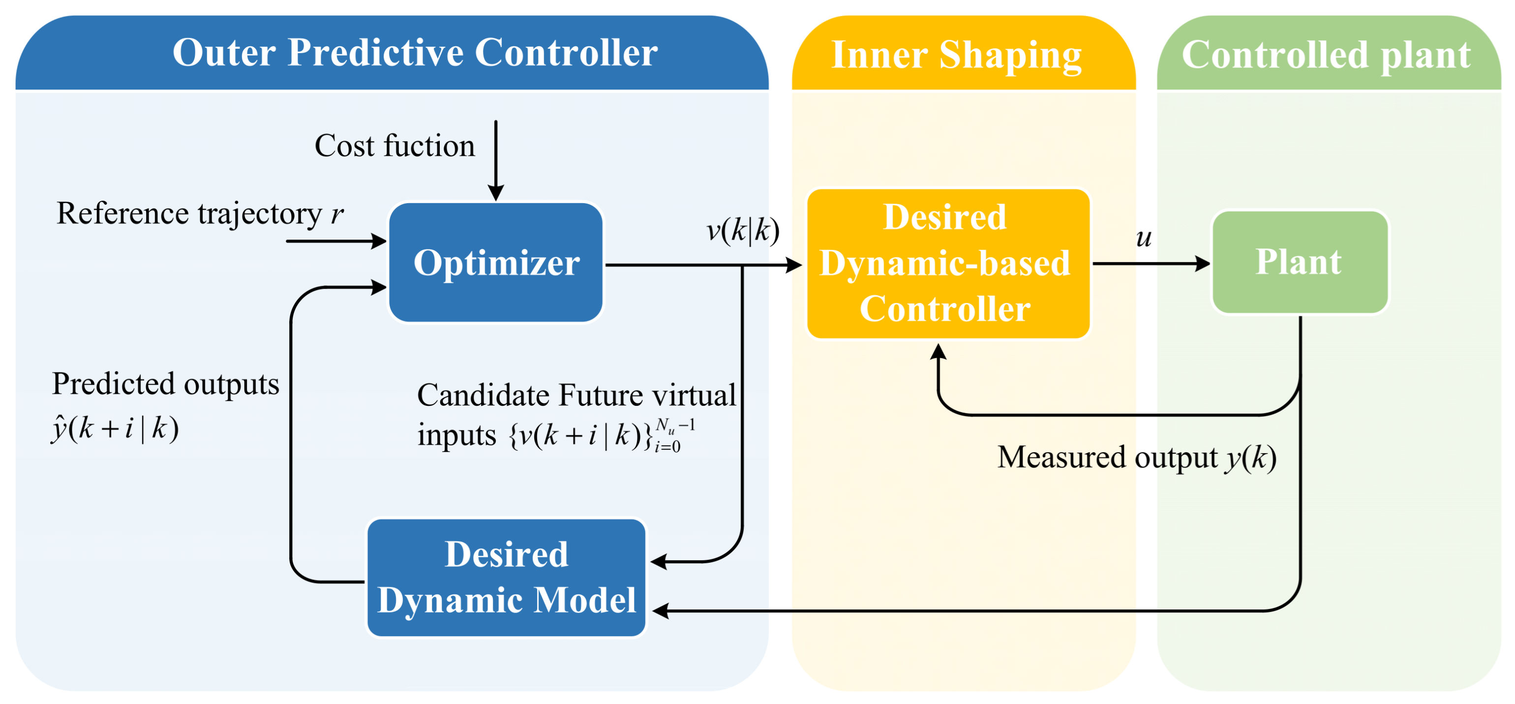
To alleviate the direct dependence of standard MPC on the raw prediction model of the plant, this work proposes a desired-dynamics-based predictive control (DDPC) framework, as shown in Figure 1. Different from robust or adaptive MPC schemes that improve uncertainty handling mainly at the optimization layer, DDPC enhances robustness through architectural conditioning: an inner desired-dynamics layer is introduced before the outer receding-horizon optimizer, such that the optimizer acts on a shaped equivalent model rather than on the raw uncertain plant.

The resulting controller has a two-layer structure. The inner layer estimates and compensates for the lumped uncertainty and reshapes the plant into a prescribed dynamic form. The outer layer retains the standard MPC mechanism and computes the virtual control sequence based on the shaped equivalent model. Therefore, the essential difference between DDPC and standard MPC is not the optimization law itself but the dynamic object on which prediction and optimization are performed.

Before deriving the equivalent prediction model, the main assumptions of the proposed DDPC framework are clarified. First, the dominant uncertain effects of the plant, including parameter variations, unmodeled dynamics, and external disturbances, can be represented as a lumped-uncertainty term in the input-output description of the controlled process. Second, the inner desired-dynamics layer can compensate for the lumped uncertainty and approximately reshape the dominant input-output behavior into a prescribed low-order desired model; exact matching is not required, but the residual mismatch should remain within an acceptable range for prediction and optimization. Third, the control direction and an approximate magnitude of the input gain are available for the inner-layer implementation.

2.2. Methodology

The essence of the inner desired-dynamics structure in DDPC is to remove, as much as possible, the influence of uncertainty from the principal dynamic channel seen by the outer MPC. To address the impact of parameter disturbances, unmodeled dynamics, and external disturbances on model prediction accuracy, the inner layer isolates the primary nominal dynamics from uncertainties, making the dynamic path seen by the outer MPC layer more structured and predictable.

For general systems, consider the following single-input single-output continuous-time uncertain system:

$$\left\{\begin{array}{l}{x}^{(n)}(t)=F(t,x,\eta ,w)+g(t)u(t)\\ y(t)=x(t)\end{array}\right.$$

(1)

where $y(t)\in R$ is the measured output, $u(t)\in R$ is the control input, and $x^{(n)}(t)$ denotes the n-th time derivative of x(t). The function $F(\cdot )$ collects the uncertain and difficult-to-model dynamics, including unmodeled dynamics, parameter perturbations, and exogenous disturbances, while g(t) denotes the possibly time-varying input gain.

Let b_e denote an estimate of the input gain g(t), and let m denote the estimated system order adopted for controller design. Then, the plant can be rewritten as follows:

$$\left\{\begin{array}{l}{x}^{(m)}(t)=F(t,x,\eta ,w)+(g(t)-b_e)u(t)+b_{e}u(t)+\left(x^{(m)}(t)-x^{(n)}(t)\right)\\ y(t)=x(t)\end{array}\right.$$

(2)

Equation (2) separates the nominal input channel b_eu(t) from the remaining uncertain terms. F(t, x, η, w) represents non-ideal effects such as parametric uncertainty and unmodeled dynamics, (g(t) − b_e)u(t) reflects the input-gain mismatch, and (x^(m)(t) − x⁽ⁿ⁾(t)) accounts for the residual induced by mismatch between the estimated order and the true system order. Aggregating these terms leads to the lumped disturbance:

$$f(t)=F(t,x,\eta ,w)+(g(t)-b_e)u(t)+x^{(m)}(t)-x^{(n)}(t)$$

(3)

so that the plant admits the compact normalized representation:

$$\left\{\begin{array}{l}{x}^{(m)}(t)=f(t)+b_{e}u(t)\\ y(t)=x(t)\end{array}\right.$$

(4)

The significance of (4) is fundamental for DDPC. Once all uncertainty-related effects are absorbed into the single channel f(t), the inner layer can be designed around two coupled objectives: (i) estimating the lumped disturbance f(t) and (ii) compensating it so that the dominant input-output dynamics are reshaped toward a desired model.

To this end, the inner layer is abstracted as a unified estimator-compensator pair:

$$\widehat{f}(t)={\mathcal{O}}_f(y(t),u(t);{\theta }_o)$$

(5)

$$u(t)={\mathcal{C}}_{dd}(v(t),y(t),\widehat{f}(t);{\theta }_c)$$

(6)

where $\widehat{f}(t)$ is the estimate of the lumped disturbance, ${\mathcal{O}}_f(\cdot )$ denotes the disturbance estimator, ${\mathcal{C}}_{dd}(\cdot )$ is the shaping control law, $v(t)\in ℝ$ is the virtual input generated by the outer-layer MPC, and ${\theta }_o$ and ${\theta }_c$ denote the associated parameter sets. This abstraction provides a common structural description for the inner-layer realizations developed later. In Section 4, both DDE-PID and ADRC are shown to fit naturally into this formulation: the former realizes (${\mathcal{O}}_f$, ${\mathcal{C}}_{dd}$) through a disturbance-estimation-driven 2-DOF PID/PI structure, whereas the latter realizes the same pair through an extended state observer and a disturbance-compensating control law. The two realizations differ in implementation mechanism but share the same functional role in DDPC, namely, to estimate the lumped uncertainty and reshape the plant dynamics toward the desired model.

If f(t) can be accurately estimated and effectively compensated for, the original uncertain plant in (5) is no longer directly exposed to the outer optimizer. Instead, the compensated system can be represented in the equivalent form:

$$Y(s)=G_{eq}(s)V(s)+G_{dy,eq}(s)D(s)$$

(7)

where G_eq(s) denotes the equivalent closed-loop transfer function from the virtual input v to the output y, and G_dy,eq(s) denotes the residual channel from the lumped disturbance to the output. The design objective of the inner layer is to enforce the following:

$$G_{eq}(s)\approx G_d(s)={\displaystyle \frac{{\omega }_c^m}{{(s+{\omega }_c)}^m}}$$

(8)

where G_d(s) is the desired-dynamics model and ω_c is the desired bandwidth. A derivation of the equivalent desired-dynamics model and the residual channel is provided in Appendix A.

Remark 1.

A notable feature of the inner desired-dynamics design is that the bandwidth parameter ω_c depends only on the controller parameters. It determines the speed of the closed-loop dynamics. As ω_c can be obtained explicitly at the design stage, the equivalent model used by the outer MPC is obtained, rather than through closed-loop identification.

Remark 2.

Unless otherwise stated, t denotes continuous time, k denotes the discrete sampling index, and T_s is the sampling period. Lowercase letters denote scalar signals, bold lowercase letters denote vectors, and uppercase letters denote matrices or transfer functions according to the context. The notation (∙)_k+i|k denotes the prediction at step k + i made at step k. In the DDPC framework, x and x_d denote the plant state and desired-model state, respectively; v denotes the virtual input generated by the outer MPC, u denotes the actual plant input generated by the inner shaping law, and y denotes the measured output.

In this way, the outer predictive controller is built on the equivalent model induced by the inner shaping layer. Let the state variable be as follows:

$$x_d(t)={\left[y_d(t) {\dot{y}}_d(t)\cdots y_d^{(m-1)}(t)\right]}^T$$

(9)

Then the desired dynamics G_d(s) can be described by the state-space model:

$$\left\{\begin{array}{l}{\dot{x}}_d(t)=A_d^c{x}_d(t)+B_d^{c}v(t)\\ y_d(t)=C_d^c{x}_d(t)\end{array}\right.$$

(10)

$$A_d^c=\left[\begin{array}{lllll}0\hfill & 1\hfill & 0\hfill & \dots \hfill & 0\hfill \\ 0\hfill & 0\hfill & 1\hfill & \dots \hfill & 0\hfill \\ ⋮\hfill & ⋮\hfill & ⋮\hfill & \ddots \hfill & ⋮\hfill \\ 0\hfill & 0\hfill & 0\hfill & \dots \hfill & 1\hfill \\ -\left(\begin{array}{c}m\\ 0\end{array}\right){\omega }_c^m\hfill & -\left(\begin{array}{c}m\\ 1\end{array}\right){\omega }_c^{m-1}\hfill & -\left(\begin{array}{c}m\\ 2\end{array}\right){\omega }_c^{m-2}\hfill & \dots \hfill & -\left(\begin{array}{c}m\\ m-1\end{array}\right){\omega }_c\hfill \end{array}\right]$$

$$C_d^c={\left[\begin{array}{cccc}1& 0& \dots & 0\end{array}\right]}_{ 1\times m}$$

where $\left(\begin{array}{c}m\\ i\end{array}\right)={\displaystyle \frac{m!}{i!(m-i)!}}$. When m = 2, $A_d^c$ degenerates into the following:

$$A_d^c=\left[\begin{array}{cc}0& 1\\ -{\omega }_c^2& 2{\omega }_c\end{array}\right]$$

(11)

Equation (10), after discretization with sampling period T_s, yields the following:

$$\left\{\begin{array}{l}{x}_d(k+1)=A_d{x}_d(k)+B_{d}v(k),\\ y_d(k)=C_d{x}_d(k),\end{array}\right.$$

(12)

$$A_d=e^{A_d^c\cdot T_s},B_d={\displaystyle {\int }_0^{T_s}{e}^{A_d^c\cdot \tau }\cdot B_d^c d\tau },C_d=C_d^c$$

Over a prediction horizon N_p, the stacked prediction can be written compactly as follows:

$$\mathrm{Y}(k)=\Psi x_d(k)+\Theta \mathrm{V}(k)$$

(13)

where V(k) is the stacked virtual-input sequence, $\Psi$ is the free-response matrix, and $\Theta$ is the dynamic matrix:

$$\Psi =\left[\begin{array}{c}{C}_d{A}_d\\ C_d{A}_d^2\\ ⋮\\ C_d{A}_d^{N_p}\end{array}\right] \Theta =\left[\begin{array}{lllll}{C}_d{B}_d\hfill & 0\hfill & 0\hfill & \dots \hfill & 0\hfill \\ C_d{A}_d{B}_d\hfill & C_d{B}_d\hfill & 0\hfill & \dots \hfill & 0\hfill \\ C_d{A}_d^2{B}_d\hfill & C_d{A}_d{B}_d\hfill & C_d{B}_d\hfill & \dots \hfill & 0\hfill \\ ⋮\hfill & ⋮\hfill & ⋮\hfill & \ddots \hfill & ⋮\hfill \\ C_d{A}_d^{N_p-1}{B}_d\hfill & C_d{A}_d^{N_p-2}{B}_d\hfill & C_d{A}_d^{N_p-3}{B}_d\hfill & \dots \hfill & C_d{A}_d^{N_p-N_u}{B}_d\hfill \end{array}\right]$$

(14)

The outer-layer MPC then solves the following:

$$\underset{{\mathrm{V}}^{\ast }(k)}{\min } J(k)={(\mathrm{Y}(k)-{\mathrm{Y}}_r(k))}^{T}Q(\mathrm{Y}(k)-{\mathrm{Y}}_r(k))+\mathrm{V}{(k)}^{T}R\mathrm{V}(k)$$

(15)

subject to (14), where Y_r(k) is the stacked reference trajectory, and Q ≥ 0, R ≥ 0 are weighting matrices. Only the first element of V*(k) is applied as the virtual command v(k):

$$v(k)=E_1{\mathrm{V}}^{\ast }(k),E_1=\left[\begin{array}{cccc}1& 0& \cdots & 0\end{array}\right]$$

(16)

and the actual plant input u(k) is subsequently generated by the inner shaping law:

$$u(k)=C_{dd}(v(k),y(k),\widehat{f}(k))$$

(17)

Therefore, DDPC preserves the standard receding-horizon loop of MPC while relocating the main robustness enhancement to the structural layer preceding the optimizer. The resulting online implementation is summarized in Algorithm 1.

Algorithm 1: Implementation of DDPC.

Offline setup design stage:

1. Select the inner desired-dynamics controller according to the implementation environment, DDE-PID or ADRC.

2. Choose the order of the desired-dynamics controller according to the plant order and specify a first-order or second-order desired model accordingly.

3. Determine the desired-dynamics model Gd(s) using the desired-dynamics tuning procedure; this step is performed online at design stage.

4. Construct the state-space model of Gd(s), discretize it with sampling period Ts, and obtain (Ad, Bd, Cd).

5. Build the prediction matrices Ψ and Θ, and specify the prediction horizon Np, weighting matrices Q and R.

Online implementation stage:

1. Measure the current output y(k) and update the inner estimator.

2. Estimate the lumped disturbance f(k), update the desired-model state xd(k), and predict future outputs over the horizon using (13).

3. Solve the finite-horizon optimization problem (15).

4. Extract the first virtual control move and generate the actual plant input through the inner shaping law.

5. Apply u(k) to the plant, shift the horizon forward, and repeat at the next sampling instant.

3. Inner Desired-Dynamics Realizations

To make the DDPC framework operational, the inner layer must provide two functions simultaneously: estimation of the lumped uncertainty and enforcement of a prescribed closed-loop model. In this work, these two functions are realized by two alternative structures, namely DDE-PID and ADRC. Although their internal mechanisms differ, both are used here for the same purpose: to transform the raw uncertain plant into an equivalent closed-loop system whose dominant dynamics are explicitly shaped toward the desired model G_d(s). The former emphasizes implementation compatibility with standard PID-based industrial platforms.

3.1. DDE-PID Realization

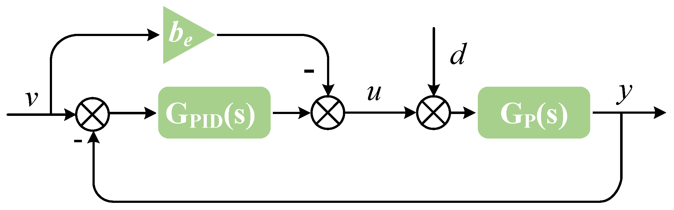
For the inner desired-dynamics layer, a convenient realization is the DDE-PID structure (Figure 2), which originates from the linearized Tornambè controller but can be rearranged into a standard 2-DOF PID form [26]. This property makes it well suited to DDPC: the controller is designed from the prescribed desired dynamics, while the final implementation remains PID-compatible for practical deployment.

Using the virtual command v generated by the outer MPC, the DDE-PID inner control law is written as follows:

$$u=(h_0\left(v-y\right)-h_1\dot{y}-\widehat{f})/b_e$$

(18)

where $\widehat{f}$ is the estimate of the lumped disturbance. The sign of b_e should be consistent with the steady-state gain of the plant.

The disturbance estimate is generated by the following:

$$\widehat{f}=\xi +k\dot{y}$$

(19)

$$\dot{\xi }=-k\xi -k^2\dot{y}-k{b}_{e}u$$

(20)

where ξ is an auxiliary observer state, and k is the observer gain. To make the disturbance-estimation dynamics faster than the prescribed closed-loop response while avoiding extra independent tuning freedom, k is linked to the desired bandwidth as follows:

$$k=10{\omega }_c$$

(21)

Substituting (19) into (18) gives the following:

$$u=-(\xi +k\dot{y})/b_e-[h_0(y-v)+h_1\dot{y}]/b_e$$

(22)

By rearranging (18)–(22), the DDE−PID law can be expressed in the equivalent 2-DOF PID form:

$$u=K_{P}e+K_I{\displaystyle \int e}dt+K_D\dot{e}-[(h_1+k)\dot{v}+k{h}_{1}v]/b_e$$

(23)

with

$$e=y_r-y, K_P=(h_0+k{h}_1)/b_e, K_I=k{h}_0/b_e, K_D=(h_1+k)/b_e,b=k{h}_1/b_e(\dot{v}=0)$$

(24)

where h₀ > 0 and h₁ > 0, and they can be parameterized using ω_c:

$$h_0={\omega }_c^2,h_1=2{\omega }_c$$

(25)

If the desired model G_d(s) is first-order, the same derivation degenerates naturally into a 2-DOF PI realization.

3.2. ADRC Realization

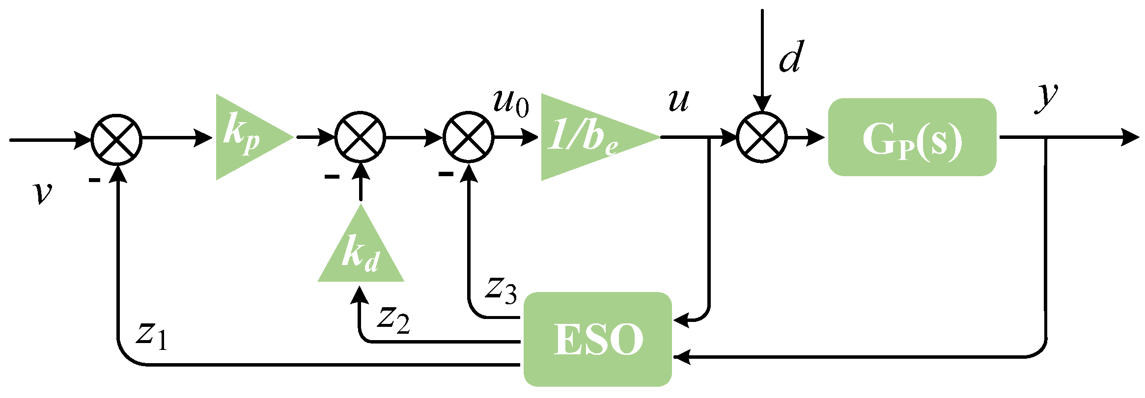
As an alternative inner-layer realization, ADRC can also be used to enforce the prescribed desired dynamics, as shown in Figure 3. Its key idea is to estimate the lumped uncertainty online through an extended state observer (ESO) and compensate for it directly in the control law [6], so that the raw plant is reshaped into the desired closed-loop form.

For the general system (4), a second-order estimated model is adopted:

$$x_1=y,\hspace{1em}{x}_2=\dot{y},\hspace{1em}{x}_3=f$$

(26)

so that the system can be written as follows:

$$\left\{\begin{array}{l}{\dot{x}}_1=x_2\\ {\dot{x}}_2=x_3+b_{e}u\\ {\dot{x}}_3=\dot{f}\end{array}\right.$$

(27)

A linear ESO is then designed as the following:

$$\left\{\begin{array}{l}{\dot{z}}_1={\dot{z}}_2-{\beta }_1(z_1-y)\\ {\dot{z}}_2={\dot{z}}_3-{\beta }_2(z_1-y)+b_{e}u\\ {\dot{z}}_3=-{\beta }_3(z_1-y)\end{array}\right.$$

(28)

where $z = (z_1,{ z}_2, z_3{)}^{\mathrm{T}}$ is the estimated extended state vector. To reduce tuning freedom, the observer gains are parameterized by the observer bandwidth ${\mathsf{\omega }}_o$ through the following:

$${\lambda }_o(s)=s^3+{\beta }_1{s}^2+{\beta }_{2}s+{\beta }_3={(s+{\omega }_o)}^3$$

(29)

which gives

$${\beta }_1=3{\omega }_o,\hspace{1em}{\beta }_2=3{\omega }_o^2,\hspace{1em}{\beta }_3={\omega }_o^3$$

(30)

To ensure that disturbance estimation is faster than the target closed-loop response while avoiding excessive noise amplification, ${\mathsf{\omega }}_o$ is linked to the desired bandwidth ${\mathsf{\omega }}_c$ by the following:

$${\omega }_o=10{\omega }_c$$

(31)

Using the virtual command v generated by the outer MPC, the ADRC shaping law is chosen as the following:

$$u_0=k_p(v-z_1)-k_d{z}_2$$

(32)

$$u=(u_0-z_3)/b_0$$

(33)

The control law is parameterized by control bandwidth ${\mathsf{\omega }}_c$ through the following:

$$k_p={\omega }_c^2,\hspace{1em}{k}_d=2{\omega }_c$$

(34)

When the ESO converges sufficiently fast,

$$z_1\to y,\hspace{1em}{z}_2\to \dot{y},\hspace{1em}{z}_3\to f$$

(35)

the residual term becomes small, and the closed-loop system approaches the following:

$$\ddot{y}+k_d\dot{y}+k_{p}y=k_{p}v$$

(36)

Compared with DDE-PID, ADRC provides a more explicit observer-based implementation of disturbance rejection, but both realizations are fully compatible with the unified DDPC framework in Section 3.

3.3. Desired-Dynamics Selection and Model-Matching Criterion

Although the inner-layer realizations in Section 3.1 and Section 3.2 are structurally different, the desired-dynamics selection problem can be formulated in a unified manner. For a given realization of {DDE−PID, ADRC}, the objective is to determine a realizable desired model G_d(s) and an associated controller-parameter vector θ_c such that the compensated equivalent model G_eq(s; θ_c) matches G_d(s) as closely as possible. The specific algorithm flow is as follows (Algorithm 2):

Algorithm 2: Desired-dynamics selection procedure

1. Specify the desired-dynamics structure and initial bandwidth. Select the order of Gd(s) according to the plant order: m = 1 is selected when the plant order is 1; m = 2 is selected for orders ≥ 2. If a time delay exists, Equation (8) becomes $G_d(s)={\omega }_c^m{e}^{-\tau s}/{(s+{\omega }_c)}^m$.

2. Compute the initial bandwidth ωd0 from the process response time tp and delay time τ using (37).

3. Select the inner-layer realization and generate an initial feasible parameter set. Choose the inner-layer realization {DDE-PID, ADRC} and initialize the corresponding controller-parameter vector θc. For DDE-PID, θc = {k, ωc, be}; and for ADRC, θc = {ωo, ωc, be}. Initialize ωc = ωc0, k (or ωo) = 10ωc, and then adjust be to make Geq(s) as close as possible to Gd(s), i.e., minimize the matching error EΔ (37).

4. Expand the search in the controller-parameter space. Starting from the initial feasible set, increase ωc to generate additional feasible candidates. For each candidate, update the controller parameters θc and test the corresponding realizability. Perform this step to find the desired dynamics with the fastest overshoot-free dynamic response.

To initialize the bandwidth, the initial value is computed from the following:

$${\omega }_{c0}=\left\{\begin{array}{l}3.91/(t_p-\tau )\hspace{1em}\mathrm{first-order}\\ 5.84/(t_p-\tau )\hspace{1em}\mathrm{second-order}\end{array}\right.$$

(37)

where t_p is defined as the process response time. For self−regulating processes, t_p is taken as the time required for the process response to reach 98% of its steady-state value. For non−self−regulating processes, t_p is defined as the time required for the process response to rise to 98% of the step-excitation amplitude.

To evaluate the shaping quality quantitatively, the compensated equivalent model is expressed in a multiplicative residual form as follows:

$$G_{eq}(s)=G_d(s)[1+\Delta (s)]$$

(38)

where Δ(s) denotes the multiplicative residual mismatch between the compensated equivalent model and the desired−dynamics model. When Δ(s) = 0, the compensated model coincides exactly with the desired dynamics. Based on (38), the model−matching error over the frequency range of interest is defined as follows:

$$E_{\Delta }=\underset{\omega \in \Omega }{\sup }\left|{\displaystyle \frac{G_{eq}(j\omega )}{G_d(j\omega )}}-1\right|$$

(39)

where Ω is the frequency range of interest. This index measures the maximum relative deviation of the compensated model from the desired model over the specified frequency band. A smaller E_Δ indicates that the inner-layer shaping is more accurate and that the resulting equivalent model is better suited for the outer MPC.

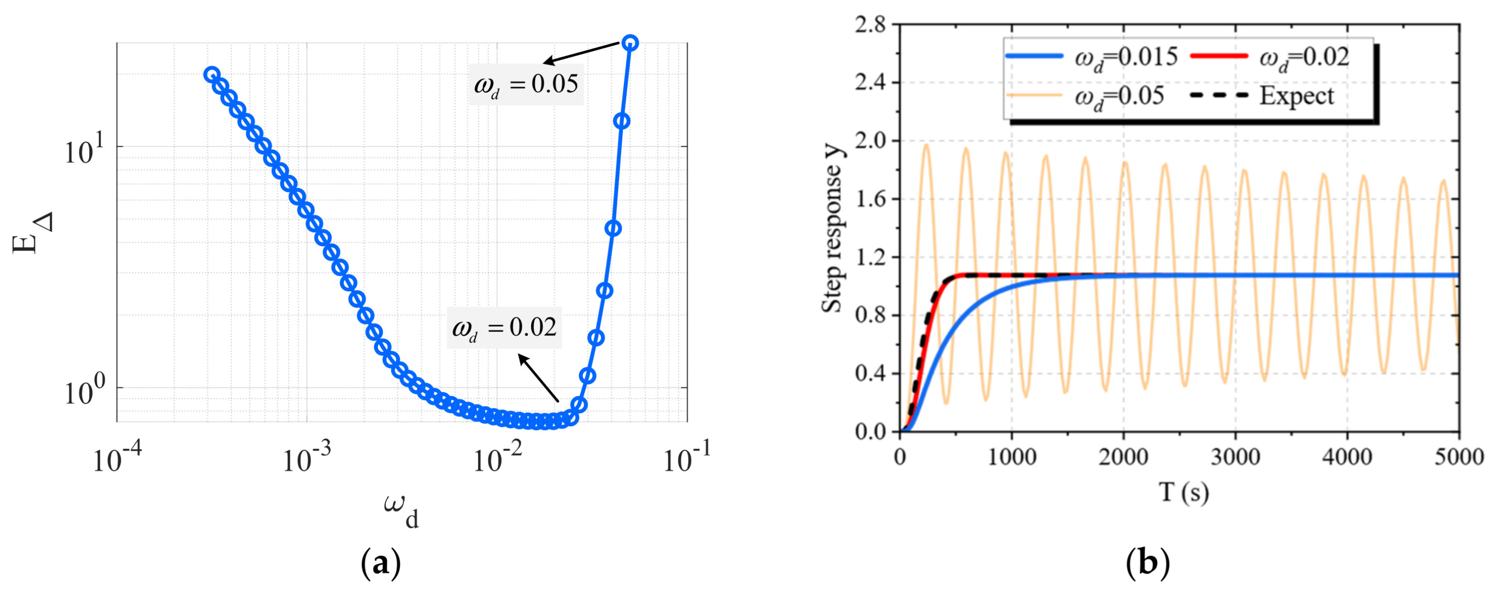
A representative example of the desired dynamics−selection result is shown in Figure 4. The model-matching error exhibits a distinctly non-monotonic dependence on the desired bandwidth ω_d (Figure 4a). When ω_d is too small, the desired model becomes overly conservative. As ω_d increases, the matching error decreases and reaches a minimum. When ω_d is further increased, the response speed becomes faster, but the mismatch rises again, indicating that the desired dynamics become too aggressive. The choice of desired bandwidth determines the trade-off between response speed and model feasibility. The corresponding time−domain responses are shown in Figure 4b, which is consistent with the trend of E_Δ.

In practice, the desired bandwidth ω_d is selected through a step-test-based model-matching procedure. Around the operating point, a small-amplitude step is then applied to the virtual input, and the inner-layer parameters are adjusted so that the measured shaped response follows the desired dynamic curve under the current ω_d. After an acceptable match is obtained, ω_d is gradually increased, and the matching procedure is repeated. During the step-test-based tuning process, the influence of ω_d on stability margin is assessed through the matching quality between the shaped response and the desired curve. A small ω_d produces a conservative response and preserves a larger margin against unmodeled high-order dynamics, time delay, input-gain mismatch, and measurement noise. Increasing ω_d accelerates the response but also requires faster disturbance estimation and stronger control action. Once ω_d exceeds the realizable range of the inner layer, E_Δ increases, and the response may show overshoot, oscillation, or excessive control variation, indicating a reduced effective stability margin. Therefore, the selected ω_d is the largest bandwidth that keeps the shaped response close to the desired trajectory while maintaining smooth and non-oscillatory control behavior.

3.4. Uncertainty Contraction Effect

To quantify the uncertainty-contraction effect induced by the inner desired-dynamics layer, an uncertain plant family with parametric perturbations is considered. The nominal plant is chosen as the following:

$$G_p={\displaystyle \frac{K}{(T_{1}s+1)(T_{2}s+1)}}$$

(40)

with independent parameter variations described by the following:

$$K\in K_0(1\pm \delta ),T_1\in T_{10}(1\pm \delta ), T_2\in T_{20}(1\pm \delta )$$

(41)

where δ denotes the perturbation level. For each member of the uncertain plant family, the same inner desired-dynamics shaping law is applied, and the resulting equivalent closed-loop family is compared with the original one in the time domain.

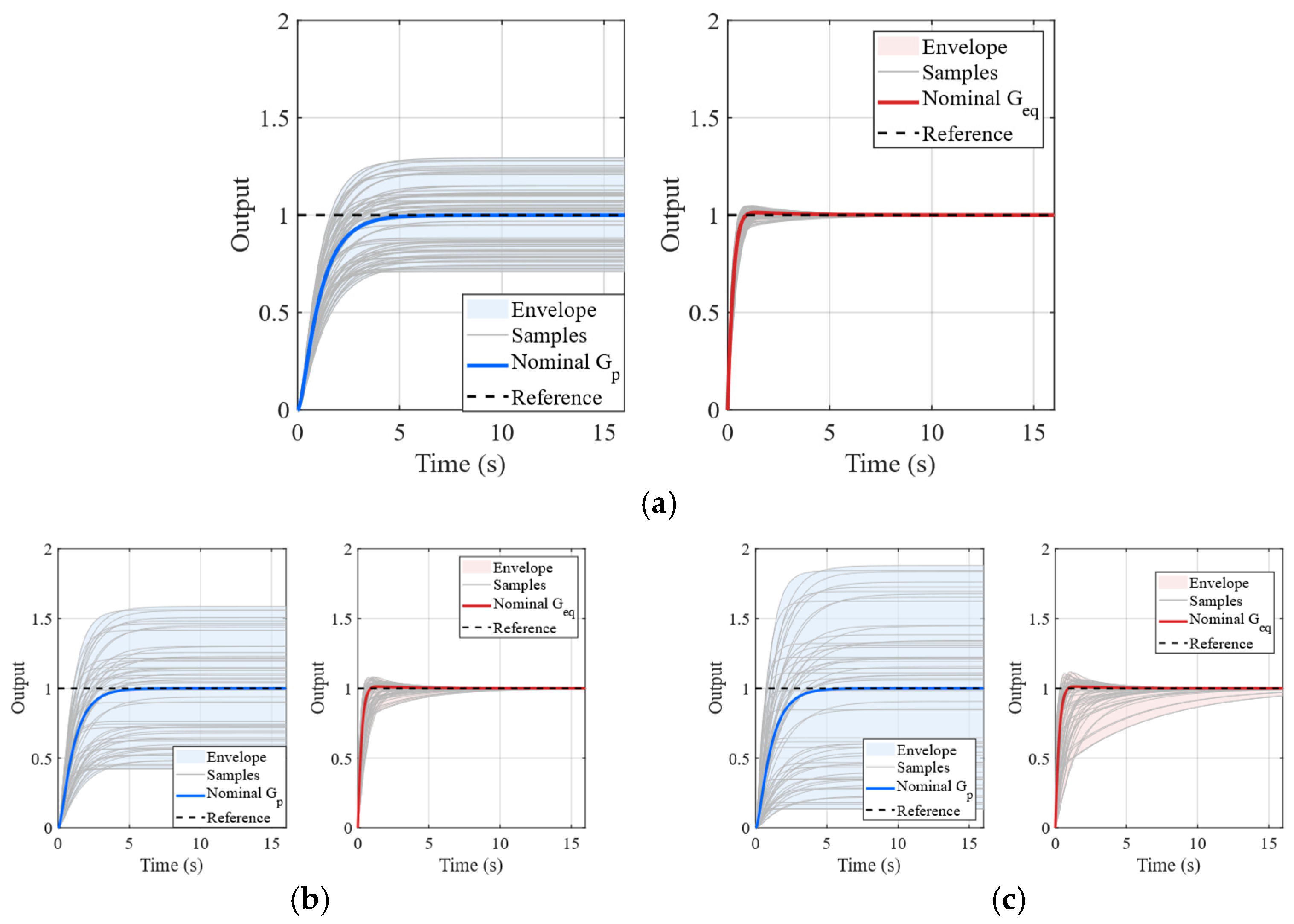
Figure 5 shows the step-response envelopes of the original plant family and the shaped equivalent family under three perturbation levels, namely δ = 0.3, 0.6, and 0.9. Before shaping, the responses of the original plant family exhibit significant dispersion in both transient and steady-state behavior, and the envelope broadens rapidly as the uncertainty level increases. This indicates that the raw plant uncertainty is directly reflected in the dominant dynamic channel.

After inner-layer shaping, the equivalent closed-loop responses collapse into a much narrower neighborhood around the reference dynamics. For all three perturbation levels, the shaped family shows substantially reduced response dispersion and a markedly tighter step-response envelope. Even when δ increases to 0.9, the equivalent family remains much more concentrated than the corresponding original family. This demonstrates that the inner desired-dynamics layer not only modifies the nominal closed-loop form but also weakens the propagation of plant uncertainty to the main channel seen by the outer predictive controller. As a result, the predictive model perceived by the outer MPC becomes more coherent across plant perturbations, which reduces prediction mismatch, weakens sensitivity to modeling errors, and enlarges the admissible uncertainty range.

4. Simulation Research, Frequency-Domain Analysis, and Robustness Testing

This section evaluates DDPC through a staged validation procedure. Linear, nonlinear, and multivariable benchmarks are used to examine whether the inner desired-dynamics layer can provide the outer MPC with a more consistent prediction object under model mismatch, parameter perturbation, and loop coupling. Frequency-domain analysis, estimator-gain sensitivity testing, Monte Carlo simulations, and computational-cost evaluation are then used to examine disturbance attenuation, parameter sensitivity, statistical robustness, and implementation burden.

The closed-loop performance is quantified by the integral absolute error,$\mathrm{IAE}={\int }_0^{\infty }\left|e\left(t\right)\right| \mathrm{dt}$, the total variation of the control input, TV $= {\sum }_{i=1}^{\infty }\left|u_{i+1}-u_i\right|$, the overshoot σ, and the settling time T_s. Unless otherwise specified, the outer MPC is implemented in an unconstrained quadratic form; therefore, the benchmark studies focus on prediction-object shaping, robustness, and closed-loop performance rather than hard-constraint handling.

4.1. Linear Benchmark Model

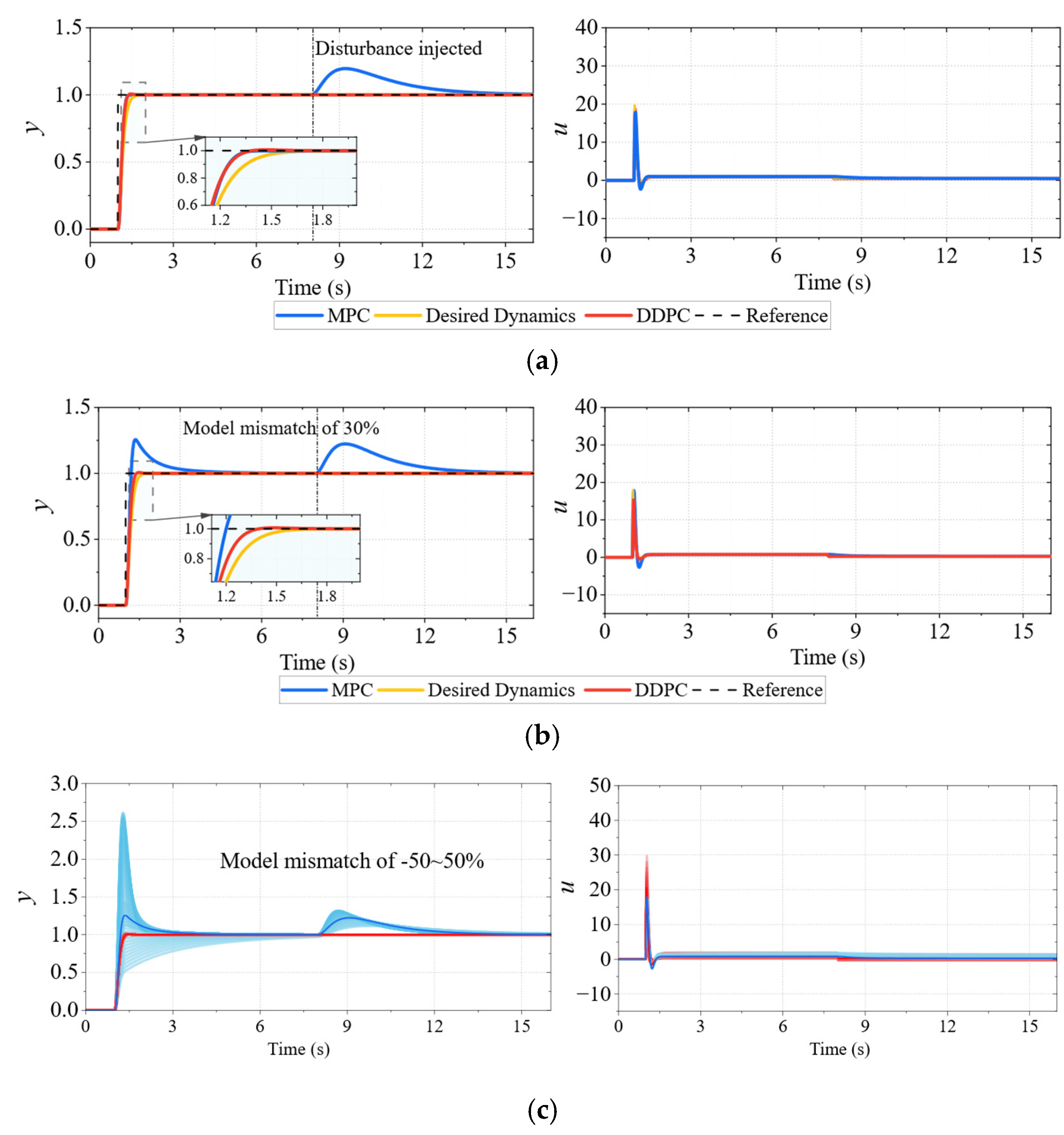
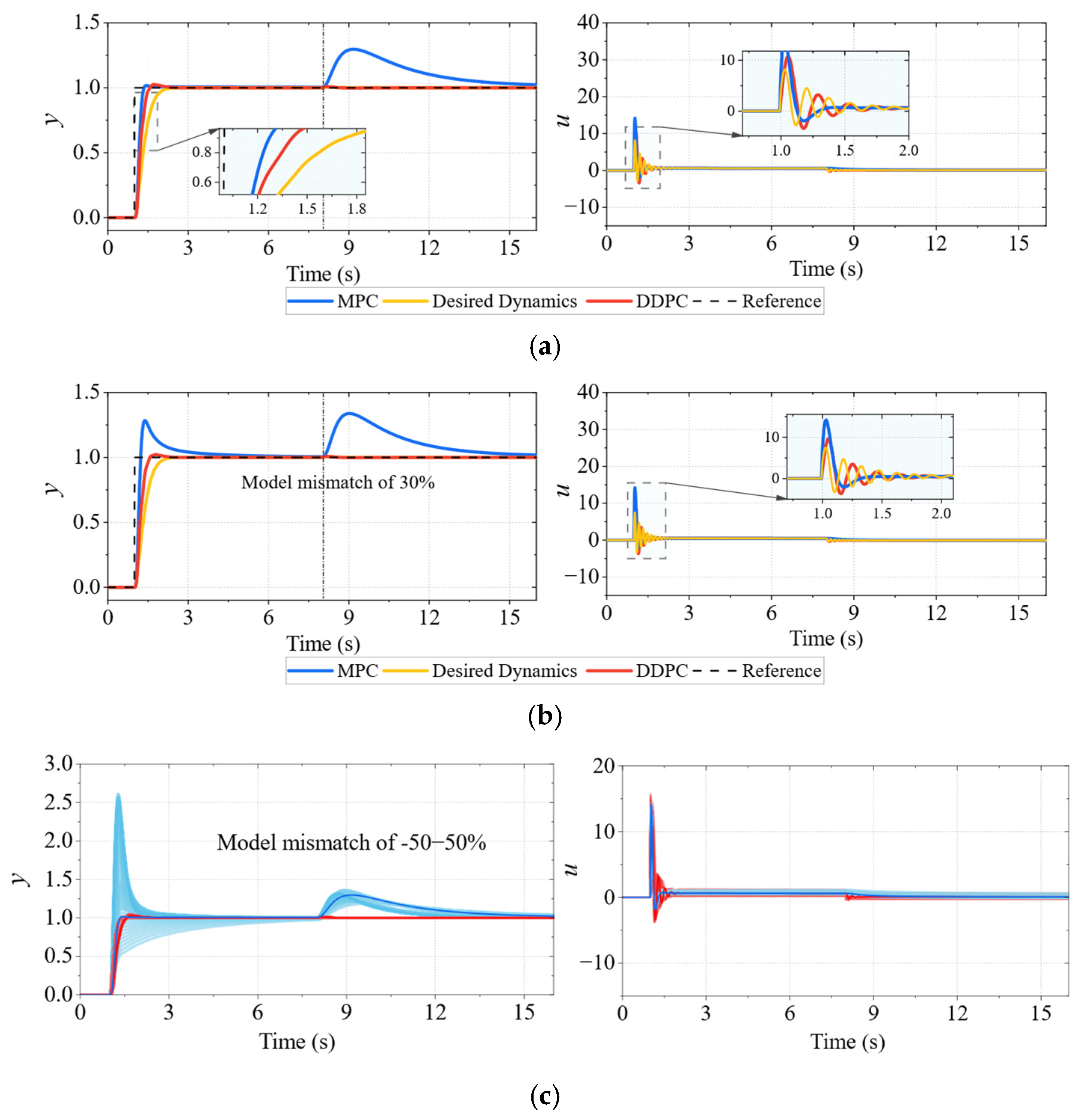
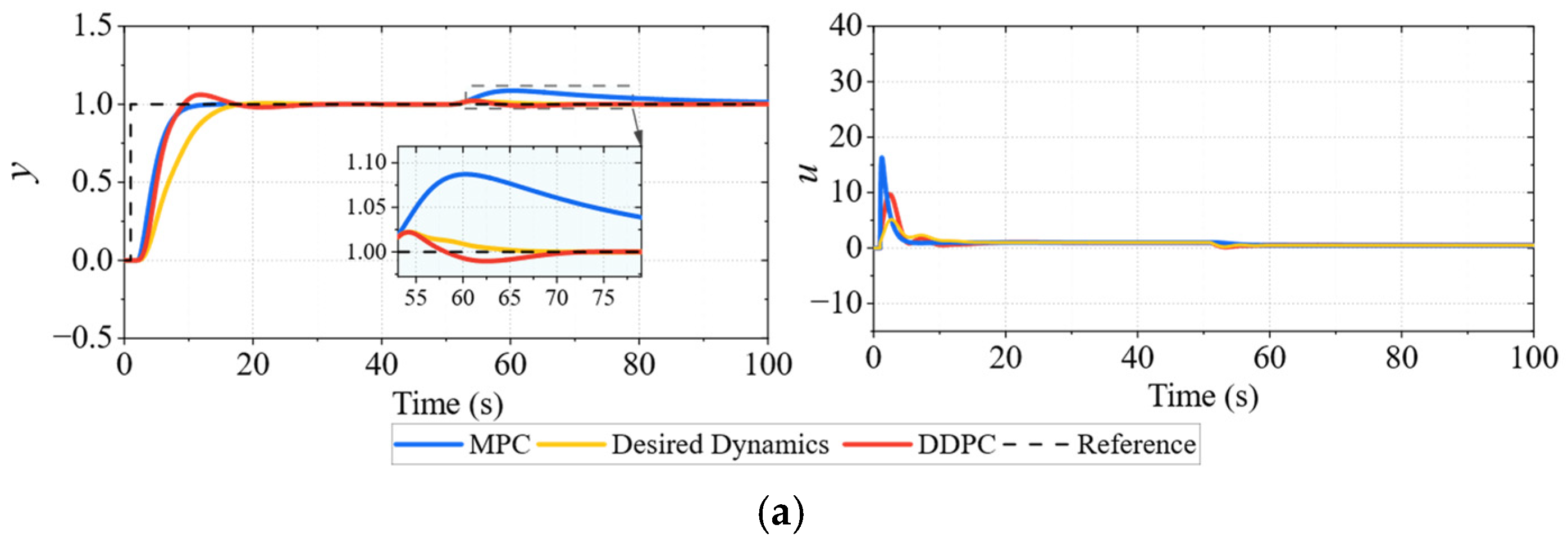
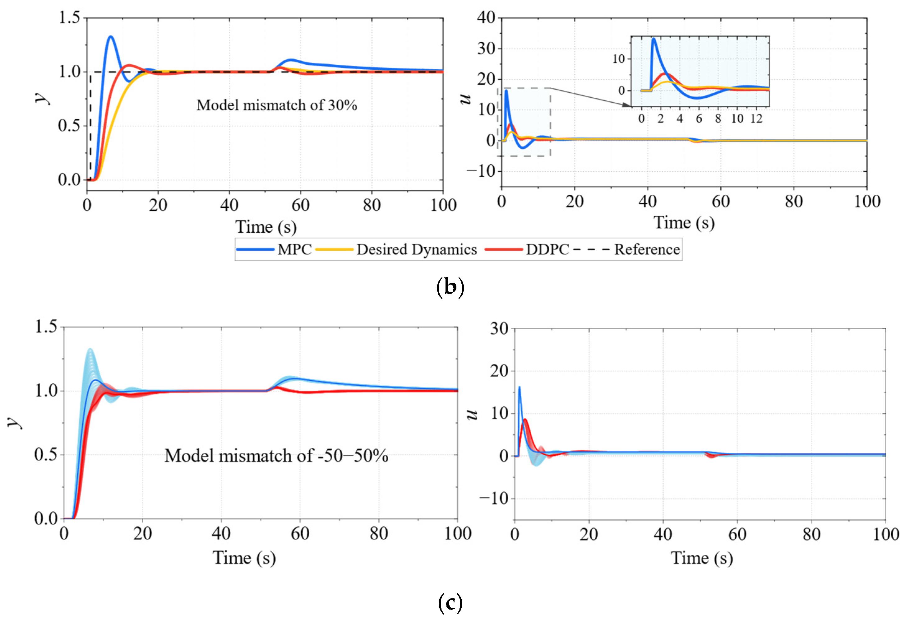
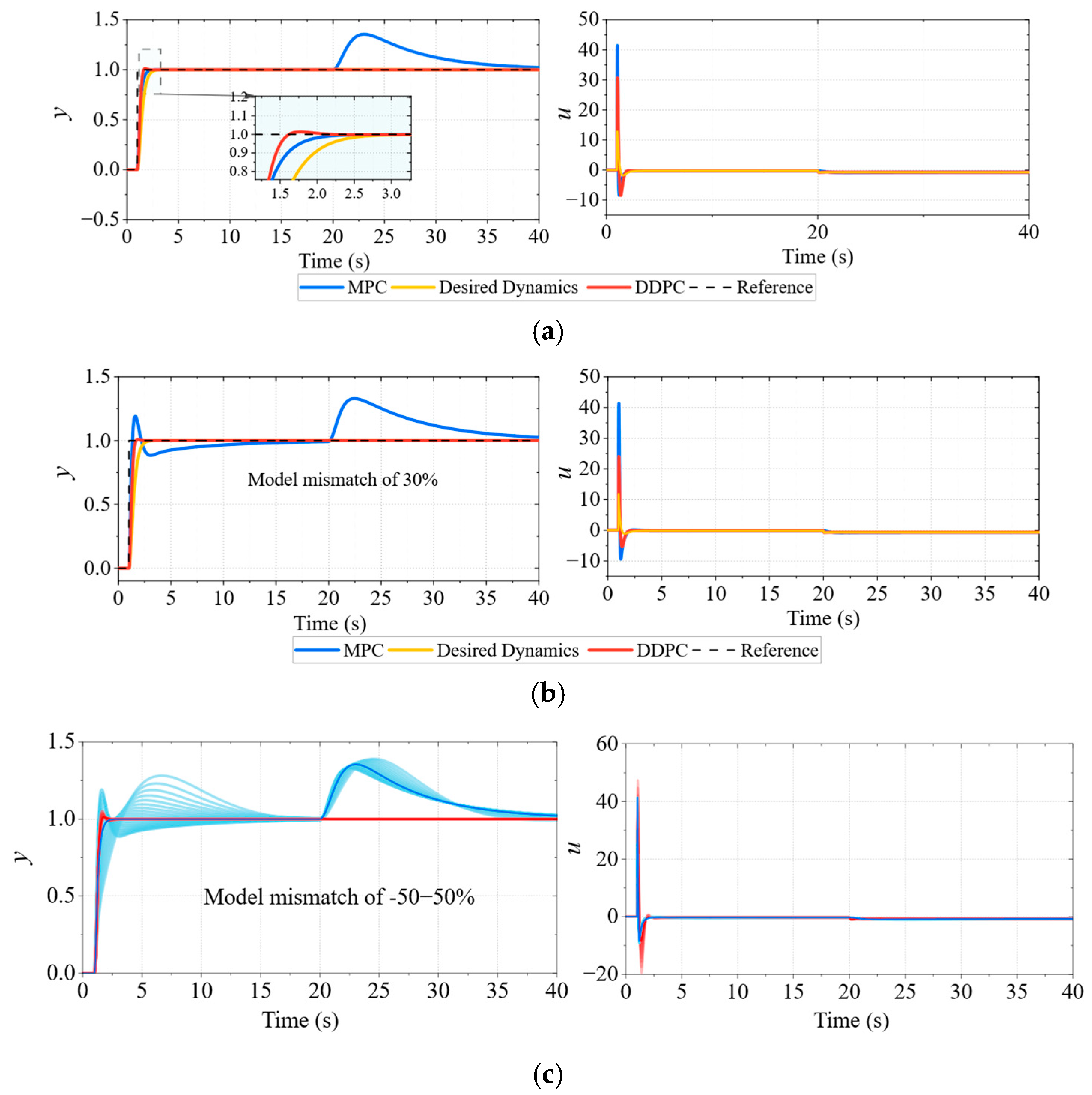
The representations of the four baseline models are shown in

Table 2. Linear benchmark processes and corresponding model-mismatch settings used in the simulation.

Plant	Nominal Model	Model Mismatch
1	$G_{p,1}(s)={\displaystyle \frac{1}{(s+1)(0.2s+1)}}$	$G_{pr,1}(s)={\displaystyle \frac{\delta }{(\delta s+1)(0.2\delta s+1)}}$
2	$G_{p,2}(s)={\displaystyle \frac{2(15s+1)}{(20s+1)(s+1){(0.1s+1)}^2}}$	$G_{pr,2}(s)={\displaystyle \frac{2\delta (15s+1)}{(20\delta s+1)(\delta s+1){(0.1\delta s+1)}^2}}$
3	$G_{p,3}(s)={\displaystyle \frac{1}{(20s+1)(2s+1)}}{e}^{-s}$	$G_{pr,3}(s)={\displaystyle \frac{\delta }{(20\delta s+1)(2\delta s+1)}}{e}^{-\delta s}$
4	$G_{p,4}(s)={\displaystyle \frac{4}{(4s-1)(s+1)}}$	$G_{pr,4}(s)={\displaystyle \frac{4\delta }{(4\delta s-1)(\delta s+1)}}$

. The results for the four linear processes are shown in Figure 6, Figure 7, Figure 8 and Figure 9, and the corresponding quantitative indices are summarized in

Table 3. Quantitative performance comparison of standard MPC, the standalone desired-dynamics controller, and DDPC for the linear benchmark processes under nominal and mismatched conditions. (Note: Smaller IAE, TV, σ, and Ts indicate better tracking accuracy, lower control activity, weaker overshoot, and faster settling, respectively. The table should be read together with the response envelopes in Figure 6, Figure 7, Figure 8 and Figure 9 to assess both nominal performance and robustness under mismatch or parameter perturbations.)

Plant/Case	Performance Indices
	Controller	IAE	TV	σ (%)	Ts (s)
Gp1/Nominal Model	Standard MPC	0.73	41.91	0	1.34
	Desired Dynamic Controller—DDE	0.18	41.38	0	1.51
	DDPC	0.17	40.19	0	1.38
Gp1/Model Mismatch	Standard MPC	0.94	42.30	25.58	3.35
	Desired Dynamic Controller—DDE	0.19	37.58	0	1.51
	DDPC	0.17	32.96	0.07	1.46
Gp2/Nominal Model	Standard MPC	1.19	33.60	1.74	1.36
	Desired Dynamic Controller—DDE	0.38	49.50	0.01	2.06
	DDPC	0.28	42.46	1.81	1.92
Gp2/Model Mismatch	Standard MPC	1.41	33.58	28.39	3.11
	Desired Dynamic Controller—DDE	0.38	60.85	0.02	2.06
	DDPC	0.25	45.22	1.19	1.85
Gp3/Nominal Model	Standard MPC	6.02	32.30	0	8.42
	Desired Dynamic Controller—ADRC	4.74	11.37	0.57	14.2
	DDPC	6.81	22.49	1.42	9.14
Gp3/Model Mismatch	Standard MPC	5.67	36.82	17.89	9.81
	Desired Dynamic Controller—ADRC	6.69	14.8	0.22	14.35
	DDPC	4.69	26.44	0	9.31
Gp4/Nominal Model	Standard MPC	3.17	100.33	0	1.90
	Desired Dynamic Controller—ADRC	0.50	49.65	0	2.18
	DDPC	0.26	78.90	0.37	1.51
Gp4/Model Mismatch	Standard MPC	3.52	101.65	9.75	9.70
	Desired Dynamic Controller—ADRC	0.50	47.43	0	2.58
	DDPC	0.26	65.17	1.09	1.53

. Overall, the simulations show that DDPC improves the consistency of the effective plant seen by the outer MPC, especially when model mismatch or parameter perturbation is present. This improvement is reflected mainly in reduced overshoot, shorter recovery time, and narrower response envelopes.

Processes 1 and 2 are used to examine whether DDPC can preserve nominal tracking performance while improving robustness under model mismatch. For Process 1, DDPC and standard MPC give comparable nominal responses. Under model mismatch, however, standard MPC produces a large overshoot of 25.58% and a settling time of 3.35 s, whereas DDPC reduces the overshoot to 0.07% and the settling time to 1.46 s. The response envelope in Figure 6c further shows that DDPC generates a much tighter trajectory family under parameter perturbations. A similar trend is observed for Process 2. Under model mismatch, DDPC reduces the overshoot from 28.39% to 1.19% and the IAE from 1.41 to 0.25. Although the TV of DDPC is higher than that of standard MPC in this case, the improved tracking and narrower response envelope indicate a practical trade-off between robustness enhancement and control activity.

Process 3 contains an explicit time delay and therefore provides a more challenging case for desired-dynamics shaping. Under nominal conditions, DDPC reduces the TV but slightly increases the IAE and settling time, indicating that the shaped dynamics may introduce a mild nominal-performance trade-off for this delayed plant. Under model mismatch, however, DDPC reduces the IAE, TV, and settling time relative to standard MPC and eliminates the overshoot. This result suggests that the main value of DDPC for delayed systems lies in improving mismatch robustness rather than uniformly accelerating the nominal response.

Process 4 represents an unstable plant and provides the clearest case in which DDPC improves both nominal and mismatched performance. Under the nominal model, DDPC reduces the IAE from 3.17 to 0.26 and shortens the settling time from 1.90 s to 1.51 s. Under model mismatch, the improvement becomes more pronounced: the IAE decreases from 3.52 to 0.26, the overshoot is reduced from 9.75% to 1.09%, and the settling time decreases from 9.70 s to 1.53 s. These results indicate that the inner desired-dynamics layer can provide a prediction object that remains informative even when the nominal plant model becomes unreliable.

At the same time, the comparison with the standalone desired-dynamics controller clarifies the contribution of the outer predictive layer: the inner layer provides the basic dynamic regularization, while the outer layer improves tracking and control coordination whenever the reshaped model remains sufficiently informative for prediction.

The main findings of the linear benchmark tests are as follows: The advantage of DDPC is most evident when the prediction model is no longer consistent with the actual plant. For the stable and high-order processes, DDPC substantially reduces overshoot and settling-time deterioration under model mismatch. For the time-delay and unstable processes, DDPC also improves robustness by suppressing response dispersion and reducing the sensitivity of the closed-loop behavior to parameter perturbations. Therefore, the linear benchmark results support the main mechanism of DDPC: the inner desired-dynamics layer provides a more coherent equivalent prediction object for the outer MPC.

In DDPC, the estimated order m denotes the design order of the desired-dynamics model. When the true order n is different from m, the residual term caused by the order mismatch is included in the lumped disturbance f(t). This treatment follows the ADRC principle, in which unknown dynamics, parameter uncertainties, and external disturbances are collectively regarded as a total disturbance and estimated by an extended state observer [6]. For high-order plants, existing studies have shown that ADRC tuning becomes more challenging, and singular-perturbation-based analyses indicate that closed-loop stability depends on the interaction between the slow feedback subsystem and the fast observer subsystem, as well as the observer bandwidth [28,29].

In the present simulations, the desired-dynamics order is selected as m = 2 for all four linear benchmark processes. Thus, Process 2, which contains higher-order dynamics, and Process 3, which contains a time-delay component, provide representative cases of dynamic-order mismatch. The results in Table 2 show that DDPC remains effective in these cases. For Process 2 under model mismatch, DDPC reduces IAE from 1.41 to 0.25 compared with standard MPC. For Process 3 under model mismatch, DDPC reduces IAE from 5.67 to 4.69 and eliminates the overshoot from 17.89% to 0.

These results indicate that moderate mismatch between the estimated order and the true plant dynamics mainly appears as an enlarged residual disturbance, leading to possible degradation in IAE, settling time, or control variation, rather than abrupt loss of closed-loop effectiveness. However, severe order mismatch may deteriorate the model-matching quality if the neglected high-order dynamics are too slow, unstable, or vary faster than the inner estimator can reconstruct.

4.2. Nonlinear Benchmark Model

To further evaluate the capability of DDPC beyond linear settings, two nonlinear benchmark processes are considered. Both are described by the general second-order form:

$$\begin{gathered} \left\{\begin{array}{l}{\dot{x}}_1=x_2\\ {\dot{x}}_2=f(x_1,x_2,t)+w(t)+bu\\ y=x_1\end{array}\right. \\ w(t)=0.5sign(\sin (t)),b=1 \end{gathered}$$

(42)

where f (⋅) characterizes the nonlinear plant dynamics, and w(t) is a bounded time-varying disturbance. The two benchmark models used in this study are summarized in

Table 4. Nonlinear benchmark processes and corresponding model-mismatch settings used in the simulation.

Plant	Model
5/Nominal Model	$G_{n5}:f={\gamma }_1\cos ({\omega }_{1}t)x_1+{\gamma }_2\cos ({\omega }_{2}t)x_2+\omega (t), {\gamma }_1={\gamma }_2=1, {\omega }_1=0.6, {\omega }_2=0.7, \omega =1$
5/Model Mismatch	$G_{nr5}:f={\gamma }_1\cos (\delta {\omega }_{1}t)x_1+{\gamma }_2\cos (\delta {\omega }_{2}t)x_2+\omega (t), {\gamma }_1={\gamma }_2=1, {\omega }_1=0.6, {\omega }_2=0.7, \omega =1$
6/Nominal Model	$G_{n6}:f={\gamma }_1\cos ({\omega }_{1}t)x_1+{\gamma }_2\cos ({\omega }_{2}t)(3-x_1^2)x_2+\omega (t), {\gamma }_1={\gamma }_2=1, {\omega }_1=0.6, {\omega }_2=0.7, \omega =1$
6/Model Mismatch	$G_{nr6}:f={\gamma }_1\cos (\delta {\omega }_{1}t)x_1+{\gamma }_2\cos (\delta {\omega }_{2}t)(3-x_1^2)x_2+\omega (t), {\gamma }_1={\gamma }_2=1, {\omega }_1=0.6, {\omega }_2=0.7, \omega =1$

. Process 5 mainly features direct modulation of the state terms by time-varying coefficients, whereas Process 6 further introduces the state-dependent multiplicative nonlinearity, resulting in a more complicated dynamic structure and stronger nonlinearity. Model mismatch is introduced by perturbing the parameter δ.

The corresponding closed-loop responses are shown in Figure 10 and Figure 11, and the quantitative performance indices are reported in Table 4. In contrast to the linear cases, the nonlinear benchmarks place a heavier burden on the prediction model itself. Accordingly, the role of DDPC here is twofold: first, to regularize the nonlinear plant into an equivalent closed-loop model with prescribed dynamics; second, to retain the predictive optimization capability of MPC on top of the shaped model. The results show that this combination is particularly beneficial when the nominal model is strongly nonlinear or when model mismatch causes rapid deterioration of standard predictive control.

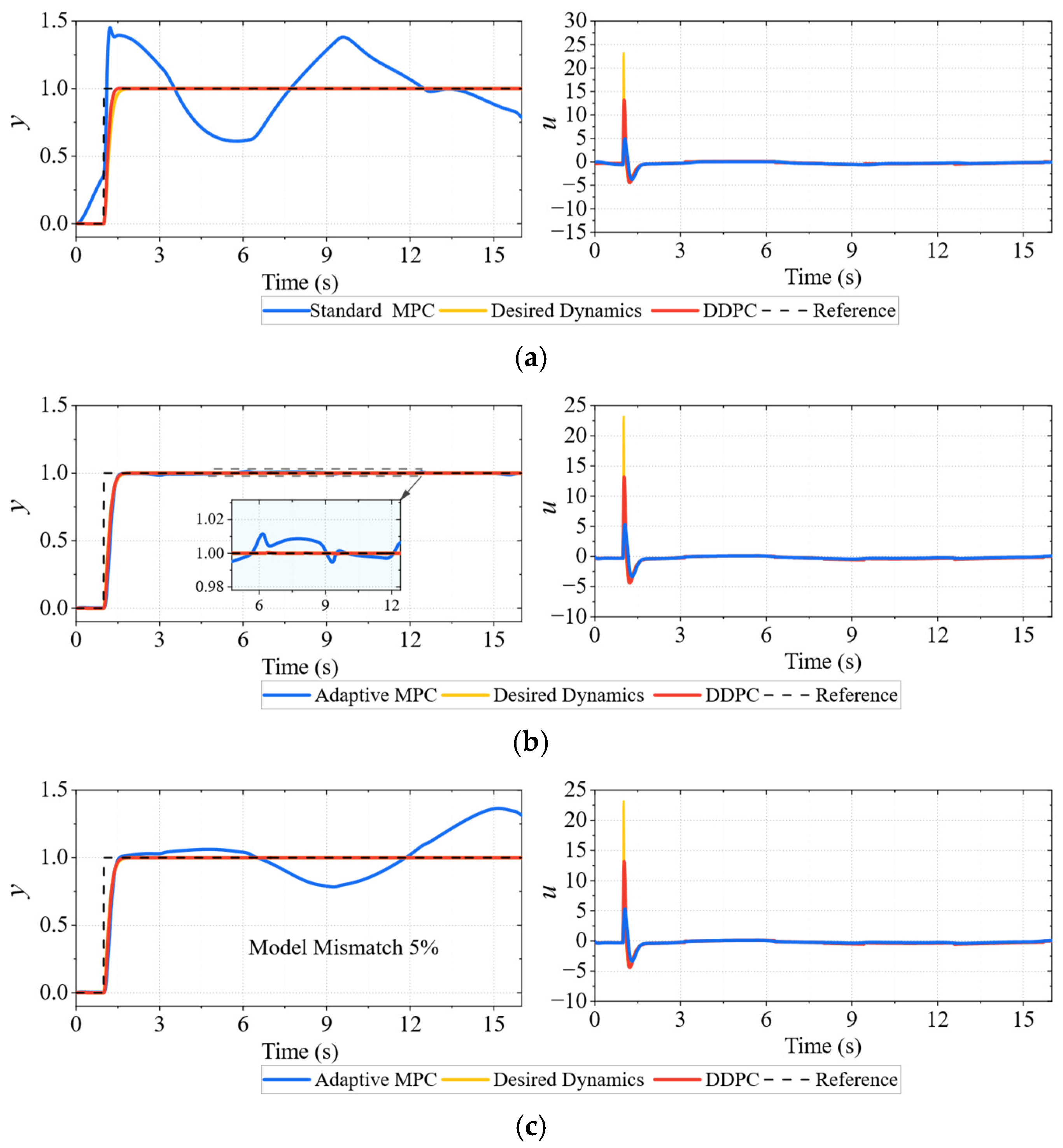
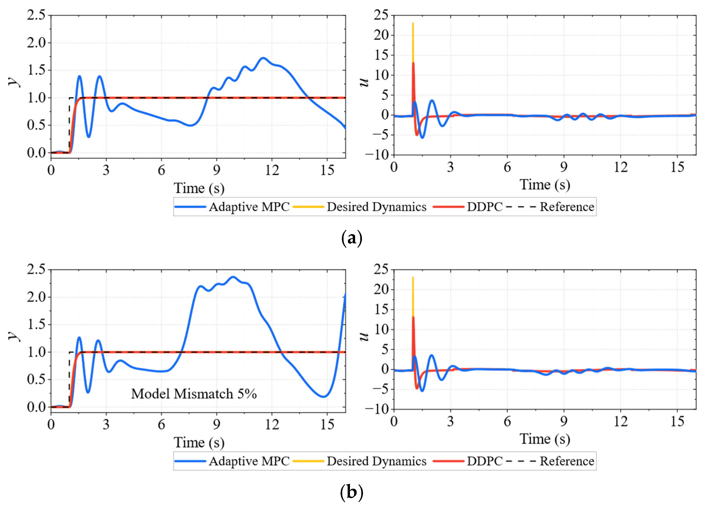
For the nominal model of Process 5, the responses in Figure 10a show that standard MPC is able to drive the output toward the reference at the initial stage, but the closed-loop response exhibits pronounced oscillations and sustained deviation from the target and fails to settle within the simulation horizon. Consistently, Table 4 shows that its IAE reaches 4.07, with an overshoot of 59.85%, while the settling time cannot be determined. This indicates that when the predictive controller acts directly on the original nonlinear time-varying process, a fixed prediction model is insufficient to represent the actual closed-loop behavior, and the prediction error accumulates continuously. In contrast, adaptive MPC significantly improves the nominal closed-loop performance, reducing the IAE to 0.31, the overshoot to 1.14%, and the settling time to about 1.56 s. This suggests that online model updating can partially alleviate the mismatch caused by time-varying dynamics. Nevertheless, DDPC still achieves the best overall performance. Its output is almost indistinguishable from the desired dynamics and the inner-loop DDE response, with the IAE further reduced to 0.21, the overshoot limited to 0.04%, and the settling time maintained at 1.55 s. It is also worth noting that the TV of DDPC is 189.32, which is higher than those of standard MPC and adaptive MPC but still substantially lower than that of the standalone DDE controller (285.63). This indicates that the proposed method achieves high tracking accuracy and strong robustness without inducing excessively aggressive inner-loop control action.

Under the 5% mismatch condition of Process 5, Figure 10c shows that the performance of adaptive MPC deteriorates markedly, and the output again exhibits obvious low-frequency oscillations and noticeable deviation around the steady-state region. According to Table 4, its IAE increases to 2.19, and the overshoot rises to 26.63%, while the settling time remains undefined within the simulation window. By contrast, DDPC preserves almost the same transient and steady-state quality before and after mismatch. Its IAE remains at 0.21, while the overshoot and settling time stay around 0.04% and 1.55 s, respectively. The TV also changes only slightly, from 189.32 to 188.77. These results demonstrate that the advantages of DDPC also apply to nonlinear characteristics. From the perspective of the external predictor, the original process is reconstructed into an approximately uniform equivalent dynamic over a relatively wide operating range, thus significantly reducing perceived uncertainty.

For the more strongly nonlinear Process 6, the superiority of DDPC over standard MPC becomes even more pronounced. As shown in Figure 11 and

Table 5. Quantitative performance comparison of standard MPC, adaptive MPC, the standalone desired—dynamics controller, and DDPC for the nonlinear benchmark processes under nominal and mismatched conditions.

Plant/Case	Performance Indices
	Controller	IAE	TV	σ (%)	Ts (s)
Gn5/Nominal Model	Standard MPC	4.07	100.31	59.85	-
	Adaptive MPC	0.31	97.39	1.14	1.56
	Desired Dynamic Controller—DDE	0.28	285.63	0.04	1.59
	DDPC	0.21	189.32	0.04	1.55
Gn5/Model Mismatch	Adaptive MPC	2.19	98.41	26.63	-
	DDPC	0.21	188.77	0.04	1.55
Gn6/Nominal Model	Standard MPC	5.23	222.35	39.36	-
	Desired Dynamic Controller—ADRC	0.22	291.19	0.04	1.59
	DDPC	0.20	154.26	0.03	1.56
Gn6/Model Mismatch	Standard MPC	8.57	207.68	116.18	-
	DDPC	0.21	193.01	0.04	1.55

, under the nominal model, the IAE, TV, and overshoot of standard MPC are 5.23, 222.35, and 39.36%, respectively. DDPC decreases the IAE by 96.18%, reduces the total variation of the control input by 30.62%, and suppresses the overshoot by 99.92%. Moreover, standard MPC fails to achieve effective settling within the simulation horizon, while DDPC maintains a settling time of 1.56 s. Under the 5% model-mismatch condition, the performance of standard MPC deteriorates further, with the IAE, TV, and overshoot increasing to 8.57, 207.68, and 116.18%, respectively. In contrast, DDPC remains at 0.21, 193.01, and 0.04%, corresponding to reductions of 97.55%, 7.06%, and 99.97%, respectively, relative to standard MPC, while the settling time is still preserved at about 1.55 s. These results demonstrate that DDPC not only substantially improves tracking accuracy and overshoot suppression but also maintains nearly unchanged closed-loop quality under model mismatch, enhancing the robustness and consistency of predictive control.

The main finding of the nonlinear benchmark tests are as follows: DDPC maintains nearly unchanged transient quality under nonlinear model mismatch, whereas the benchmark predictive controllers exhibit larger oscillation or performance deterioration. This result indicates that desired-dynamics shaping is not limited to linear perturbation cases; it also reduces the uncertainty perceived by the outer MPC when the plant contains nonlinear and time-varying components.

4.3. Nonlinear Multivariable Benchmark Model

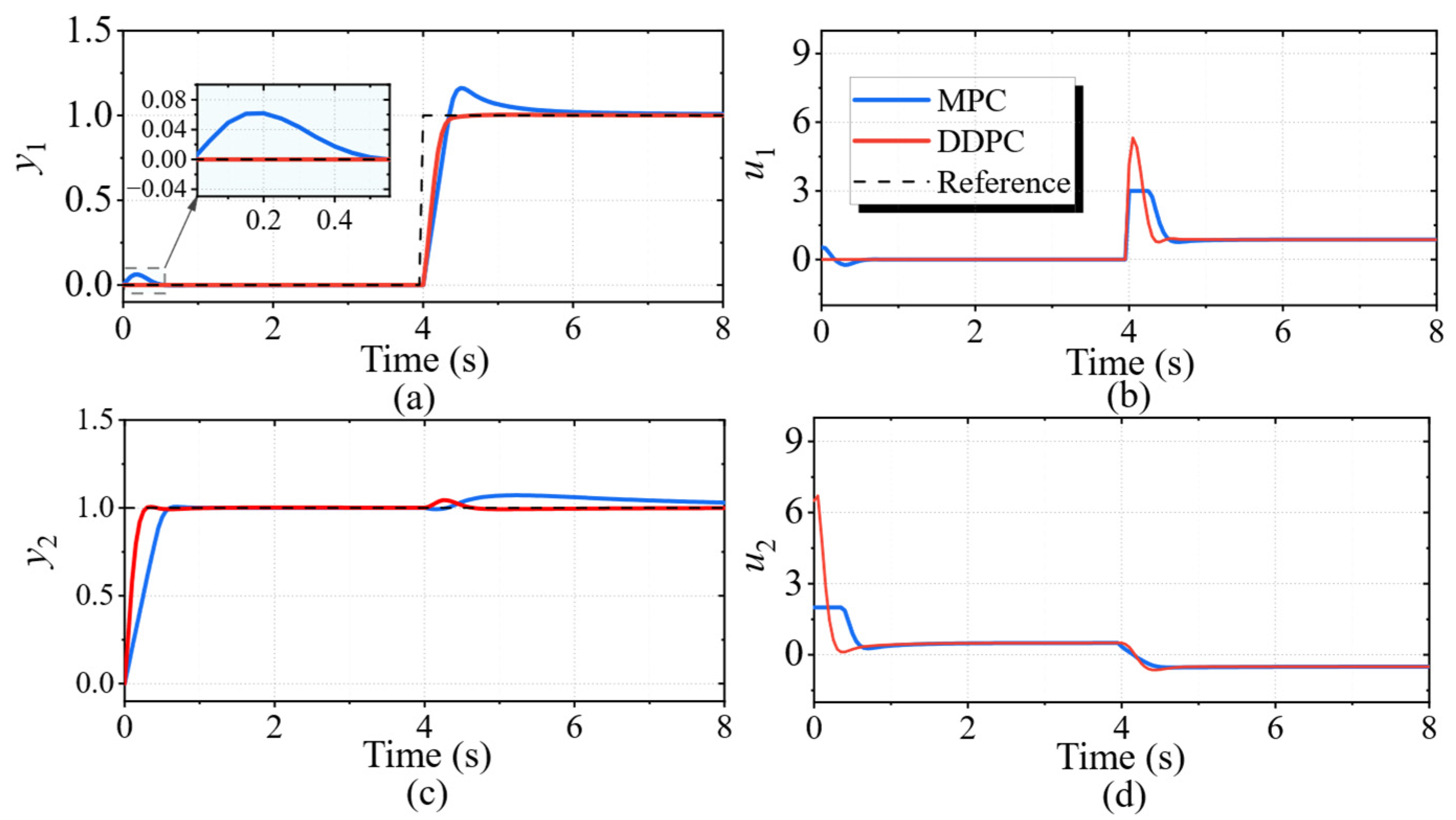
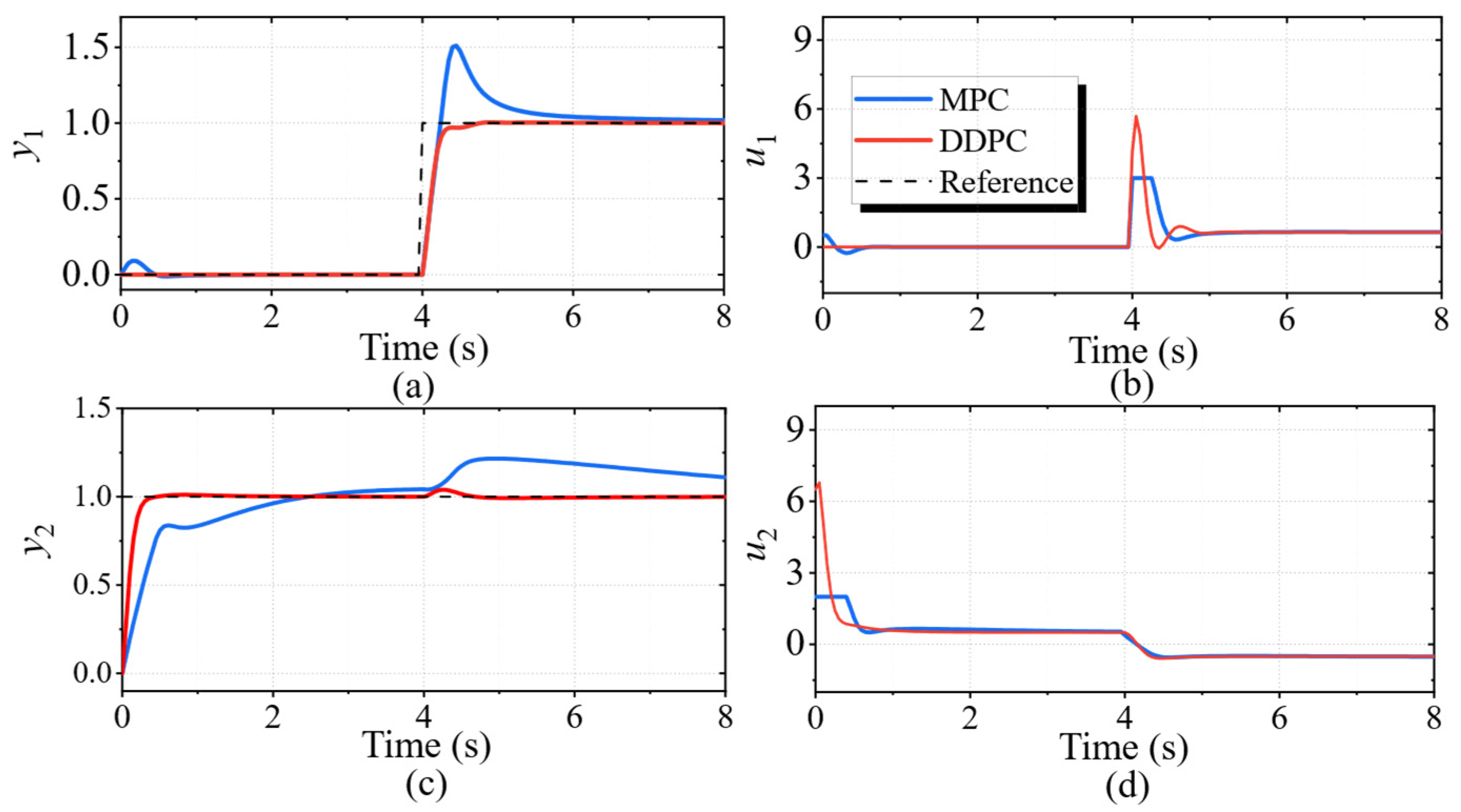
To further examine whether the proposed DDPC framework can be extended beyond single-input single-output systems, a nonlinear multivariable benchmark process is considered in this subsection. The plant is a 2 × 2 nonlinear system, whose nominal dynamics and mismatched counterpart are summarized in

Table 6. Nonlinear multi-input multi-output (MIMO) benchmark processes and corresponding model-mismatch settings.

Plant	Model
7/Nominal Model	$\left\{\begin{array}{l}{\dot{x}}_1=-x_1+u_1\\ {\dot{x}}_2=x_3\\ {\dot{x}}_3=-x_2-2x_3+x_1+0.2x_1^3+u_2\end{array}\right.\left\{\begin{array}{l}{y}_1=x_1+0.2x_1^3\\ y_2=2x_2+x_3\end{array}\right.$
7/Model Mismatch	$\left\{\begin{array}{l}{\dot{x}}_1=-x_1+u_1\\ {\dot{x}}_2=x_3\\ {\dot{x}}_3=-x_2-2\delta x_3+x_1+0.2x_1^{3\delta }+u_2\end{array}\right.\left\{\begin{array}{l}{y}_1=\delta (x_1+0.2x_1^{3\delta })\\ y_2=2\delta x_2+x_3\end{array}\right.$

. Different from the preceding SISO benchmarks, this case introduces output coupling and multivariable coordination requirements. Therefore, the comparison focuses not only on the tracking behavior of each individual output but also on whether the controller can maintain coordinated responses when one loop is disturbed by the setpoint change of the other loop.

The reference signals are arranged such that y₂ tracks a unit step from the beginning of the simulation, while y₁ is commanded to track a delayed unit step at t = 4 s. Under the nominal model, both standard MPC and DDPC achieve acceptable regulation of y₂, as shown in Figure 12. However, after the delayed step of y₁, the coupling effect becomes visible: standard MPC produces a more pronounced transient interaction between the two outputs, whereas DDPC yields a faster y₁ response with smaller overshoot and a weaker disturbance effect on y₂. This indicates that the shaped equivalent model used by DDPC provides a more consistent prediction object for coordinated multivariable optimization.

The difference becomes more evident under model mismatch. As shown in Figure 13, standard MPC exhibits a clear degradation in both channels: y1 shows a large overshoot after the delayed step, and y₂ recovers more slowly and less accurately. This behavior suggests that the nominal MIMO prediction model becomes less reliable when nonlinear coupling and model perturbation coexist. By contrast, DDPC preserves closed-loop behavior close to the nominal case. Both outputs remain near their references, and the transient interaction between the two loops is substantially reduced. Therefore, the improvement is not only reflected in individual tracking performance but also in the preservation of coordinated behavior under coupling uncertainty.

Overall, the multivariable benchmark shows that DDPC remains effective when loop coupling and nonlinear model mismatch are present. The inner desired-dynamics layer reduces the uncertainty and interaction effects exposed to the outer MPC, while the outer predictive optimizer coordinates the multivariable control actions based on the shaped equivalent model. This supports the extension of the prediction-object shaping mechanism from SISO processes to coupled MIMO systems.

4.4. Frequency-Domain Analysis

This subsection analyzes the disturbance rejection performance of the proposed DDPC method from the frequency-domain perspective. Standard MPC and the standalone desired-dynamics controller are taken as two benchmark schemes. For the desired-dynamics controller, the disturbance-to-output transfer behavior can be derived analytically from the inner-layer realization (43):

$$G_{dy,eq}(s)=\left\{\begin{array}{cc}{\displaystyle \frac{b_e[s^3+(3{\omega }_o+2{\omega }_c)s^2+(3{\omega }_o^2+6{\omega }_c{\omega }_o+{\omega }_c^2)s]G_P}{\Delta +{\omega }_c(s^3+3{\omega }_o{s}^2+3{\omega }_o^{2}s+{\omega }_o^3)G_P}}& with \mathrm{ADRC}\\ {\displaystyle \frac{G_P}{1+G_P{G}_{\mathrm{PID}}+G_P(G_{\mathrm{PID}}-l)}}& with \mathrm{DDE}\text{-}\mathrm{PID}\end{array}\right.$$

(43)

$$\begin{array}{cc}\hfill \Delta (s)& =b_e{s}^3+[b_e(3{\omega }_o+2{\omega }_c)+(3{\omega }_c^2{\omega }_o+6{\omega }_c{\omega }_o^2+{\omega }_o^3)G_P]s^2\hfill \\ & +[b_e(3{{\omega }_o^2}_2+6{\omega }_c{\omega }_o+{\omega }_c^2)+(3{\omega }_c^2{\omega }_o^2+2{\omega }_c{\omega }_o^3)G_P]s+{\omega }_c^2{\omega }_o^3{G}_P\hfill \end{array}$$

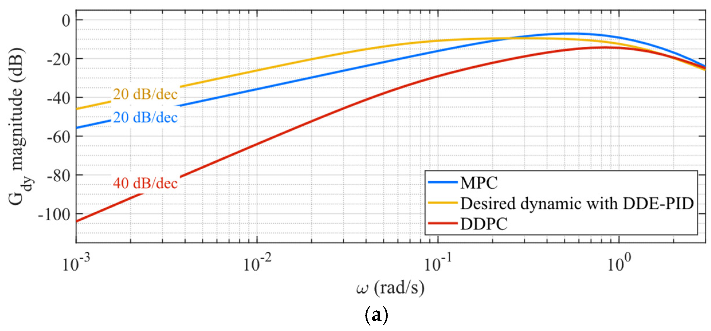
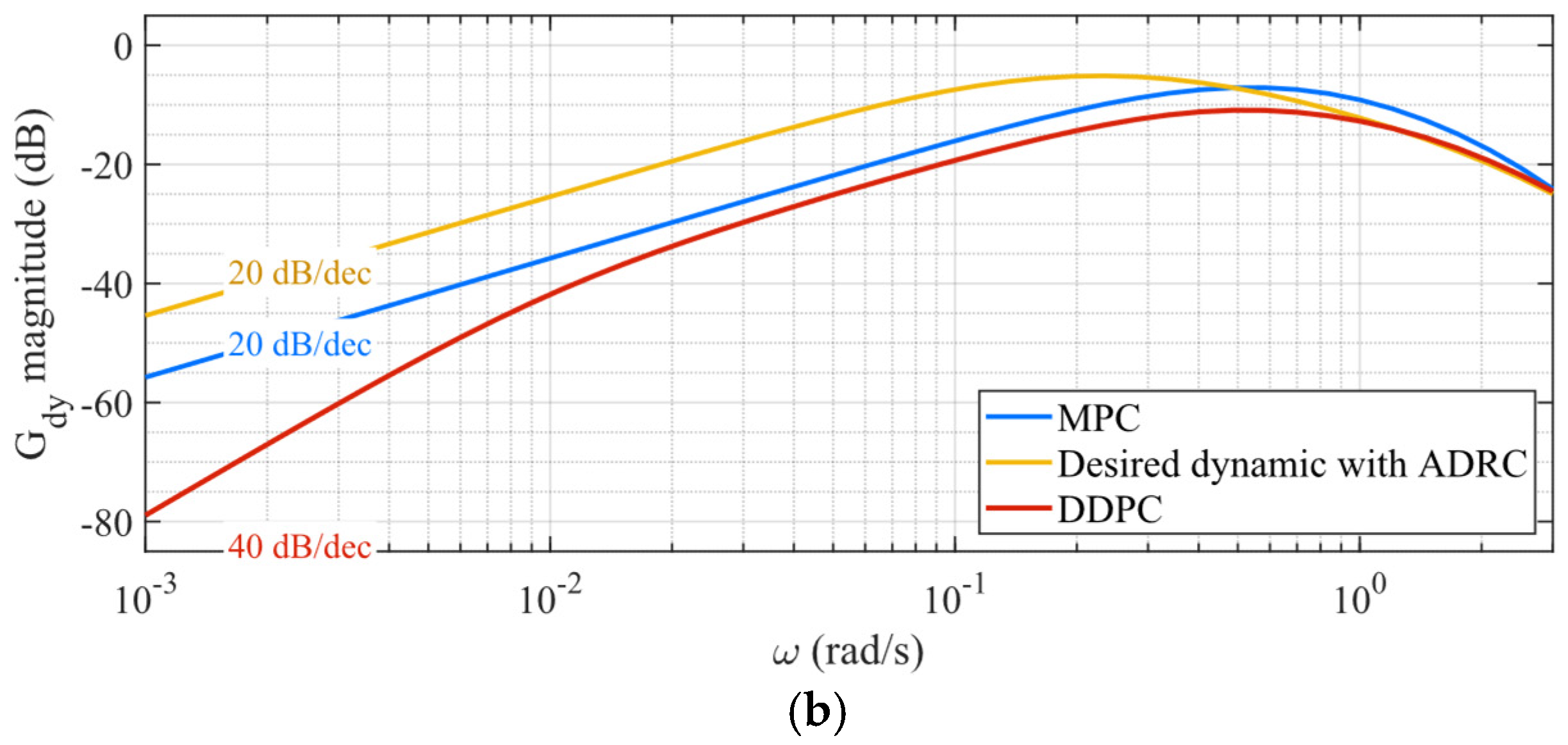
For standard MPC and DDPC, the control law is generated online through receding-horizon optimization, and a compact closed-form disturbance transfer function is generally unavailable. Therefore, the equivalent disturbance-frequency response is estimated numerically by sinusoidal injection. At each test frequency, a unit sinusoidal disturbance is injected at the plant input, while the reference is fixed at zero. After the transient vanishes, the steady-state output amplitude is extracted and normalized by the disturbance amplitude to obtain the equivalent disturbance-to-output gain. The sampling period is 0.2 s, and 45 frequency points are selected over the frequency range of interest. G_p1 is used as the test case. Standard MPC employs the original plant model for prediction, with N_p = 40, N_u = 5. The inner desired-dynamics controller is realized by either DDE-PID or ADRC, and the results are shown in Figure 14.

As shown in Figure 14, DDPC achieves a lower disturbance-response magnitude than both standard MPC and the standalone desired-dynamics controller over the low-frequency range, regardless of whether the inner layer is realized by DDE-PID or ADRC. In particular, standard MPC and the standalone desired-dynamics controller both exhibit an approximate 20 dB/dec decay rate at low frequency, whereas DDPC shows an approximate 40 dB/dec decay rate. This indicates that DDPC not only reduces the disturbance-channel gain but also increases the effective low-frequency attenuation order.

The mechanism can be analyzed as follows: In standard MPC, the disturbance is directly added at the plant input. In DDPC, by contrast, the disturbance first passes through the equivalent residual channel after inner-layer compensation. Since the inner desired-dynamics layer reshapes the plant and compresses uncertainty into a smaller equivalent residual, the outer MPC acts on a more favorable disturbance channel, leading to stronger low-frequency attenuation.

4.5. Sensitivity to Lumped-Disturbance Estimation Error

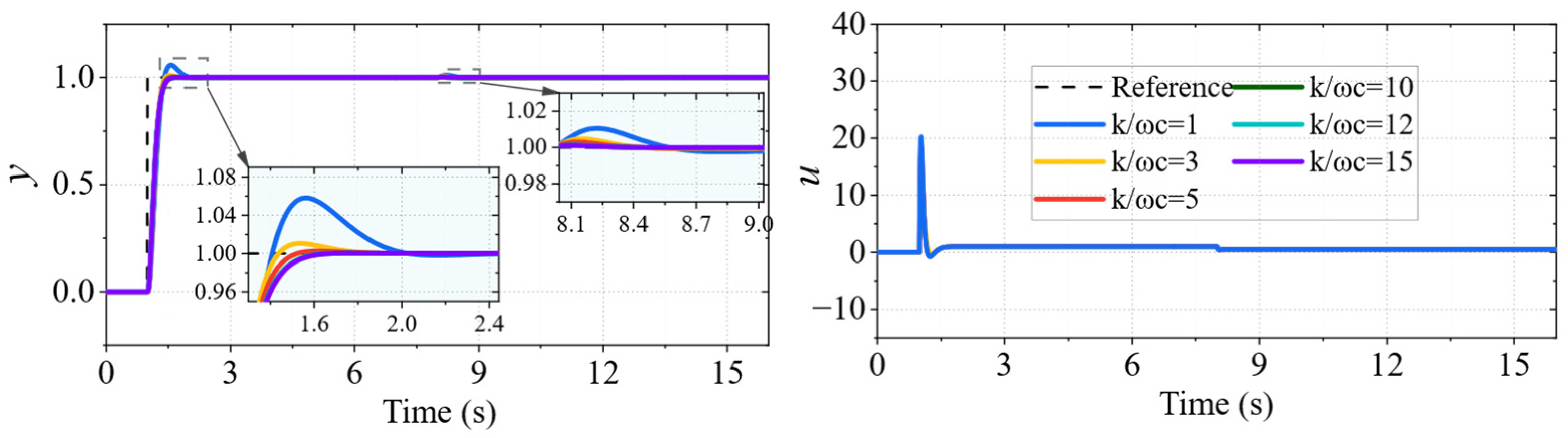
To further evaluate the practical sensitivity of DDPC to disturbance-estimation accuracy, a numerical test was conducted by varying the disturbance-estimator gain ratio k/ω_c in the DDE-PID-based DDPC realization. In this test, the desired bandwidth ω_c, MPC parameters, prediction horizon, weighting matrices, and plant condition were kept unchanged, while k/ω_c was set to 1, 3, 5, 10, 12, and 15. The corresponding closed-loop responses and quantitative indices are shown in Figure 15 and

Table 7. Sensitivity of DDPC performance to the disturbance-estimator gain ratio.

k/ωc	Performance Indices
	IAE	TV	σ (%)	Ts (s)
1	0.22	24.79	5.8	1.82
3	0.19	30.70	1.05	1.40
5	0.18	34.40	0.25	1.39
10	0.17	40.19	0	1.38
12	0.17	41.77	0	1.38
15	0.17	43.63	0	1.38

.

The results show that a small estimator gain leads to slower disturbance reconstruction and larger residual estimation error. When k/ω_c = 1, DDPC exhibits an overshoot of 5.8% and a settling time of 1.82 s. As k/ω_c increases, the tracking performance improves gradually: the IAE decreases from 0.22 to 0.17, the overshoot is eliminated, and the settling time decreases to 1.38 s when k/ω_c = 10. Further increasing it to 12 and 15 brings almost no additional improvement in output performance, while the TV increases from 40.19 to 41.77 and 43.63, respectively. This indicates that excessive estimator gain increases control activity without improving the closed-loop response. Therefore, DDPC is not critically dependent on exact lumped-disturbance estimation. Moderate estimation inaccuracies cause gradual performance degradation. The results also support the tuning rule k = 10ω_c (21), which provides a practical compromise between disturbance-estimation speed and control smoothness.

4.6. Monte Carlo-Based Probabilistic Robustness

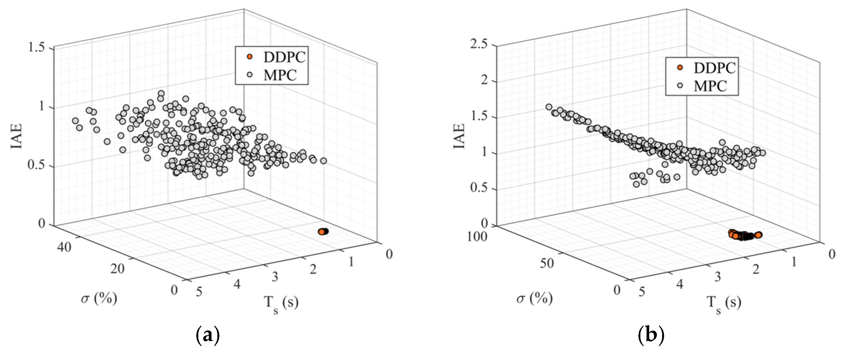
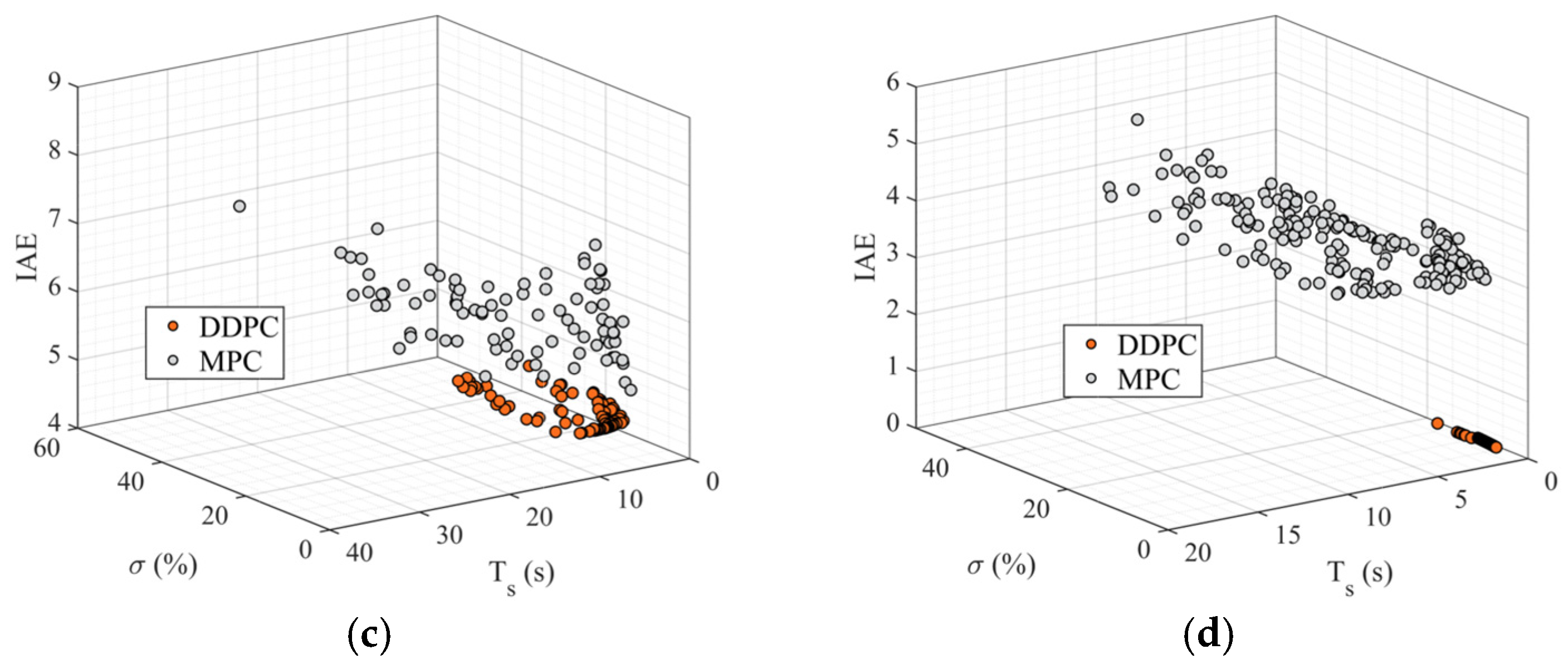
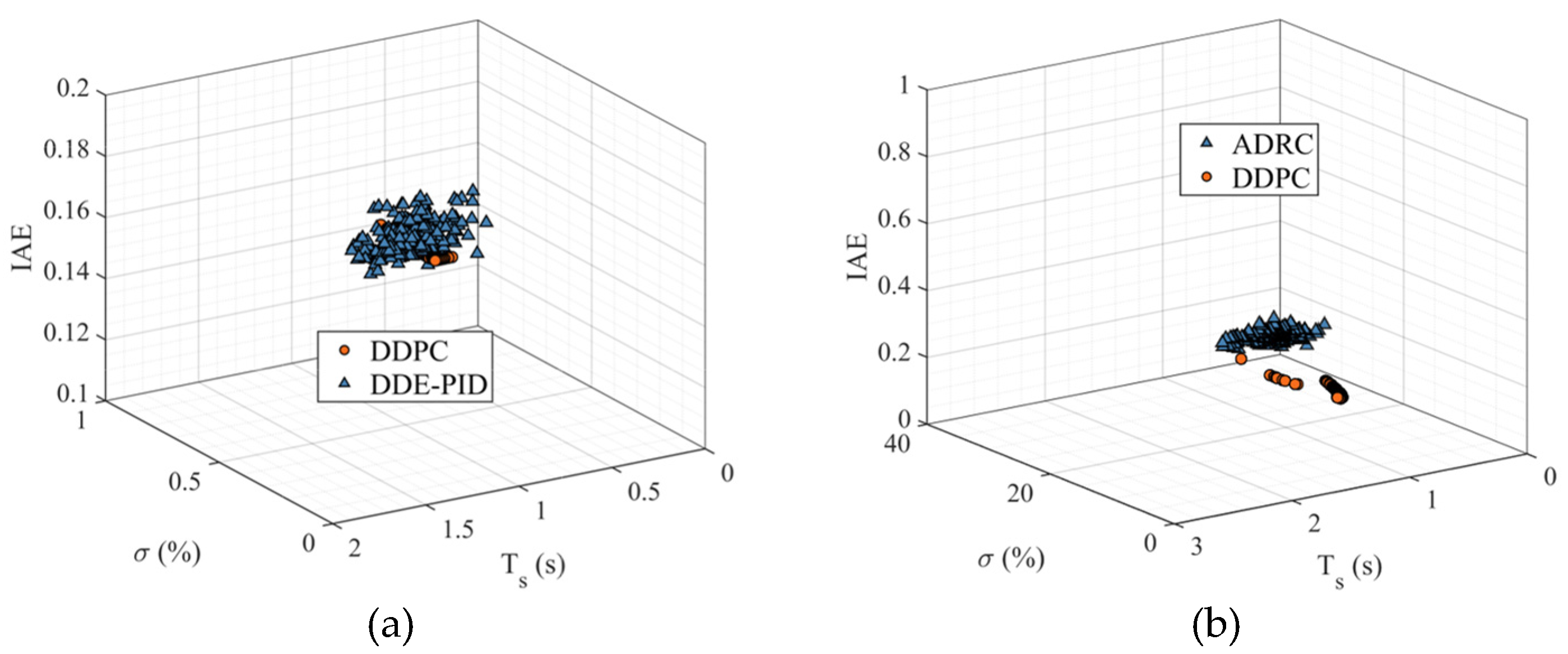
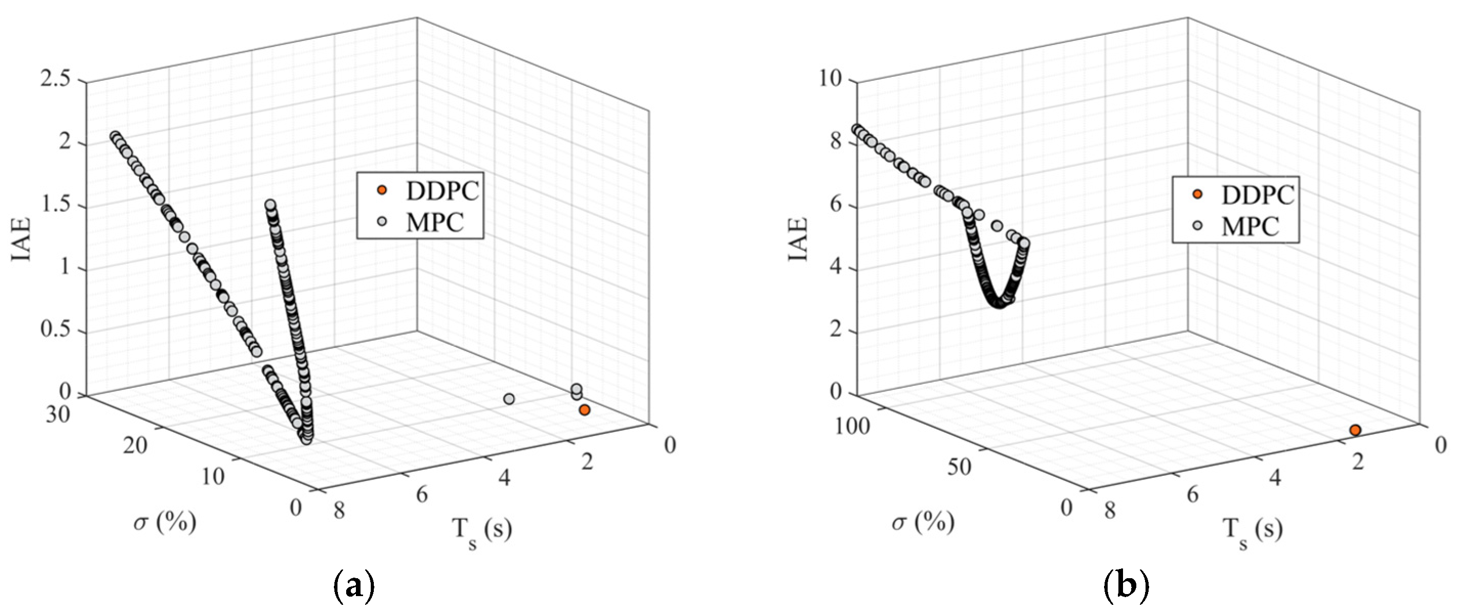
To further assess robustness from a probabilistic perspective, Monte Carlo simulations are carried out for all benchmark processes. For each plant, we randomly sampled 500 implementations with parameters within a pre-defined uncertainty range and evaluated the corresponding closed-loop response under the same control configuration. The resulting performance of each realization is characterized by IAE, the overshoot σ, and the settling time T_s. The scatter distributions of these indices provide a compact representation of robustness: a tighter and lower-valued cluster indicates that the controller is able to maintain consistent closed-loop performance over a broader range of plant variations.

The Monte Carlo results are summarized in Figure 16 for the linear benchmark processes. In all subplots, each point corresponds to one random plant realization in the performance space. The DDPC samples consistently form compact clusters located near the low-IAE, low-overshoot, and short-settling-time region, whereas the benchmark MPC samples are much more widely spread. The more compact DDPC cluster indicates that prediction-object shaping contracts the effect of parameter uncertainty into a smaller equivalent residual around the shaped model.

To further quantify the robustness improvement introduced by the outer predictive layer, two representative linear benchmarks were selected for Monte Carlo comparison against the standalone inner-layer controllers. It should be noted that DDE-PID and ADRC already provide substantial robustness enhancement by estimating and compensating for the lumped disturbance. Building on this inner-layer compensation, DDPC further incorporates predictive optimization over the shaped equivalent model. As shown in Figure 17, the DDPC samples form more compact clusters in the low-IAE, low-overshoot, and short-settling-time region, indicating that the outer predictive layer further reduces performance dispersion under parameter perturbations.

The computational cost was evaluated using 30 repeated simulations under the same computing environment. The average time per control step increases from 0.080154 ms for DDE-PID to 0.598677 ms for DDPC, corresponding to approximately 7.47 times higher computational cost due to the additional prediction and optimization layer. Nevertheless, the average online computation time of DDPC remains below 1 ms per control step, which is acceptable for the benchmark.

For the nonlinear benchmark processes, the same statistical trend is observed in Figure 18. In Figure 18a, the benchmark MPC samples for G_n5 exhibit a wide spread, indicating strong sensitivity of the nonlinear closed-loop response to parameter variation. By contrast, the DDPC samples remain concentrated in a very small neighborhood, suggesting that the inner shaping layer successfully suppresses the nonlinear uncertainty seen by the predictive optimizer. A similar but even more pronounced result is obtained for G_n6 in Figure 18b. This shows that the statistical robustness benefit of DDPC extends beyond linear perturbation analysis and remains valid for strongly nonlinear benchmark systems.

From a control perspective, the Monte Carlo results reveal an important property of DDPC: the inner desired-dynamics layer does not eliminate uncertainty but contracts its effect into a much smaller equivalent residual around the shaped model. Consequently, the outer MPC is exposed to a more coherent prediction object, and the resulting closed-loop performance becomes substantially less sensitive to plant variations. The probabilistic concentration of the DDPC samples in the three-dimensional performance space therefore provides direct statistical evidence for the uncertainty-contraction and robustness-enhancement mechanisms developed in Section 3 and Section 4.

Based on this observation, the robustness of DDPC can be further interpreted from the perspectives of stability, feasibility, and uncertainty attenuation. In terms of stability, the inner desired-dynamics layer reshapes the uncertain plant into a stable equivalent model; when ω_c > 0, G_d(s) = ${\omega }_c^m/(s+{\omega }_c{)}^m$ has stable poles, and the outer MPC performs prediction based on the discretized shaped model rather than the raw uncertain plant. In terms of feasibility, the benchmark simulations do not impose hard input/output inequality constraints, and the finite-horizon quadratic optimization problem remains solvable under the selected weighting matrices. If hard constraints are introduced, recursive feasibility should be further handled by standard MPC techniques such as soft constraints, terminal constraints, or constraint tightening. In terms of robustness, DDPC is evaluated through the model-matching error, frequency-domain disturbance attenuation, and Monte Carlo-based probabilistic performance. The frequency-domain and Monte Carlo results jointly show that DDPC contracts the effect of plant uncertainty into a smaller residual channel before the outer predictive optimization, leading to stronger disturbance attenuation and more concentrated performance distributions under parameter perturbations.

5. Control Evaluation on Coal-Fired Power Unit

Coal-fired power units operating under flexible and deep peak-shaving conditions provide a representative industrial scenario for evaluating DDPC. Under frequent load regulation, boiler thermal-control loops are affected by wide-load variations, heat-storage effects, actuator disturbances, and operating-condition-dependent dynamics, which may cause prediction mismatch when a fixed plant model is used in standard MPC. Therefore, this scenario is consistent with the motivation of DDPC: the inner desired-dynamics layer regularizes the effective plant dynamics before the outer MPC performs prediction and optimization.

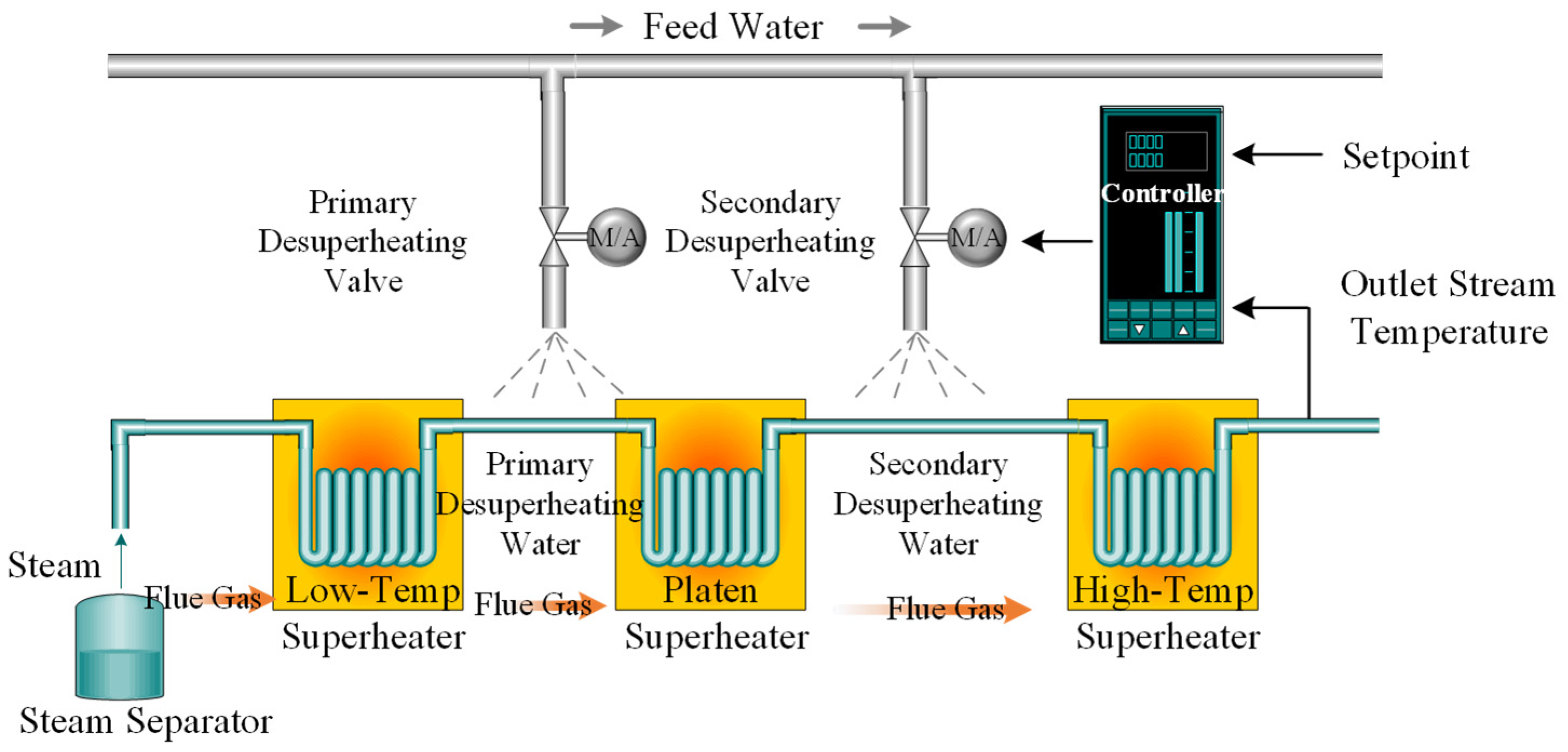
Based on this industrial background, the proposed DDPC strategy is evaluated on the superheated steam temperature control loop of a high-fidelity 660 MW coal-fired boiler hardware-in-the-loop simulator. This loop is a challenging thermal-control problem due to its large inertia, strong delay, operating-condition dependence, and strict temperature-regulation requirements. In practical operation, two stages of desuperheating are arranged between the heating surfaces to regulate the outlet steam temperature and avoid tube overheating, as shown in Figure 19. Spray water is extracted from an intermediate stage of the feedwater pump and injected through the primary and secondary desuperheating valves. The outlet temperatures downstream of the low- and high-temperature superheaters are measured and fed back to the control system, which adjusts the spray-water flow in real time to maintain the target temperature under load variations [30]. The control objective is to maintain the superheated steam temperature as stably as possible around the given value while avoiding excessive steam-temperature deviation during continuous load fluctuations.

The simulator provided by CHN Energy Zhishen Control Technology Co., Ltd. has been calibrated against operating trends from multiple real power units and can reproduce the major thermal-process dynamics of utility-scale coal-fired generation systems with high fidelity [31]. In addition, the DCS platform used in the hardware-in-the-loop tests adopts the same hardware configuration as that used in the field, which makes the validation environment closer to actual plant operation. In the present study, the controller hardware was directly connected to the simulator to form a closed loop, thereby providing a realistic validation environment between purely numerical simulation and field implementation.

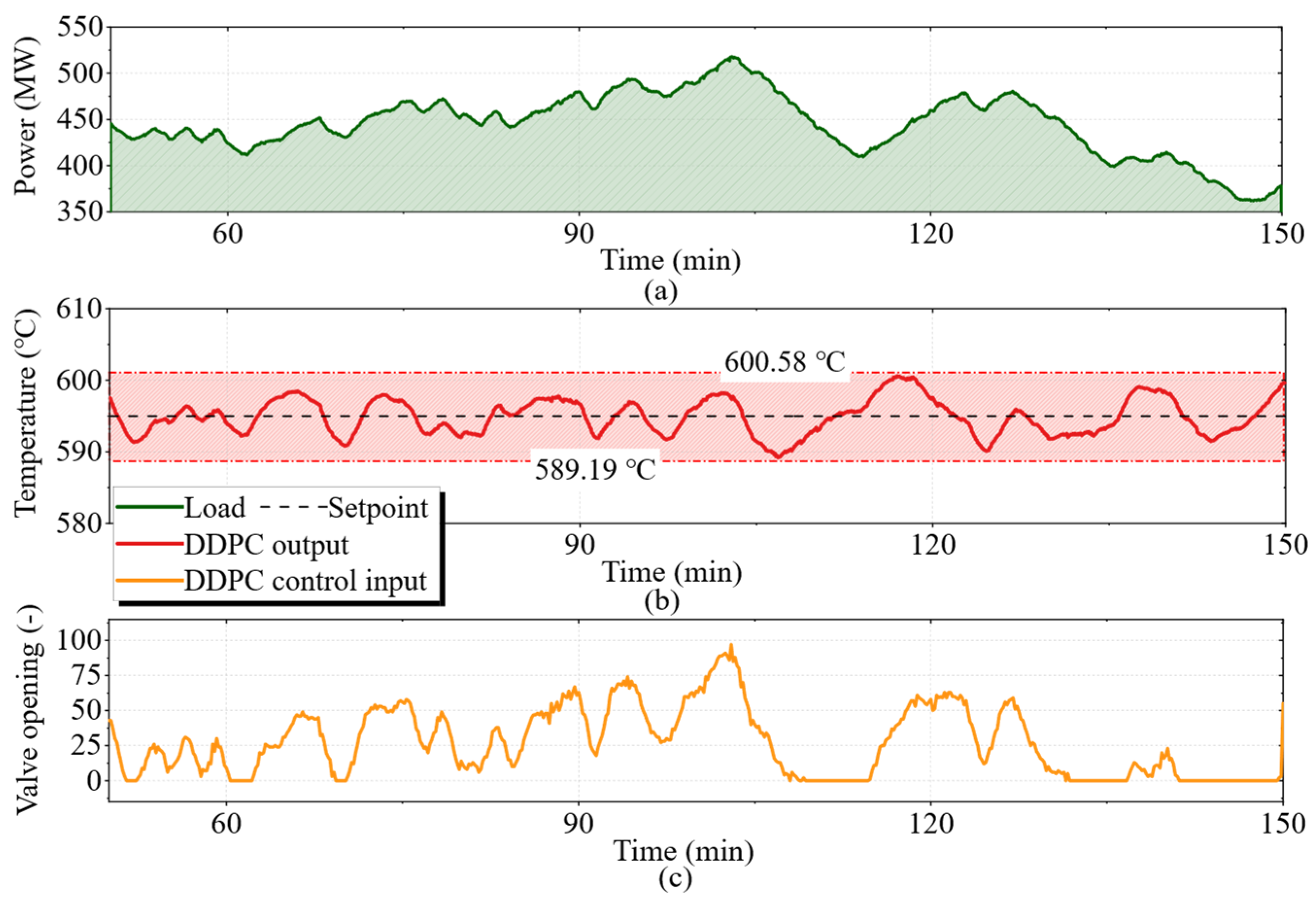
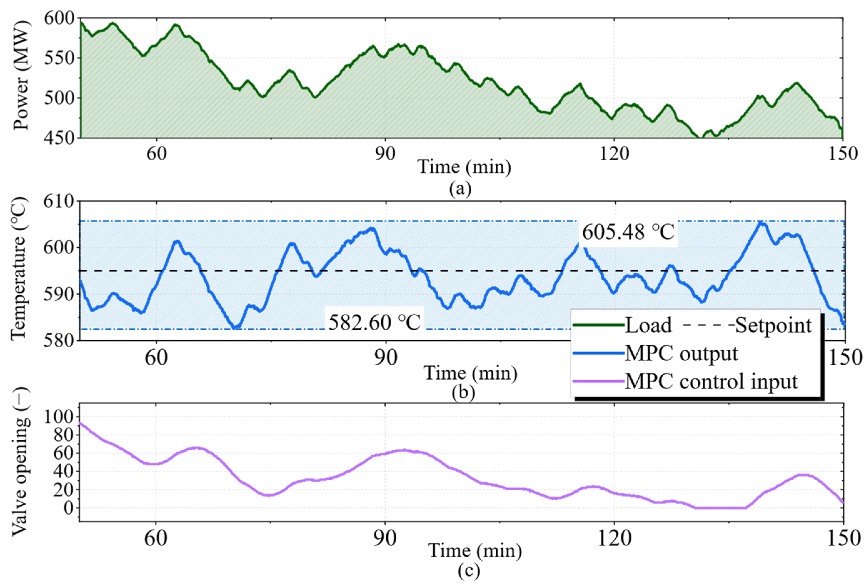
It should be noted that the load trajectories used in these hardware-in-the-loop tests were derived from real dispatch data of a power plant under deep peak-shaving operation. Therefore, the load input could not be arbitrarily reset or exactly repeated as in a purely numerical simulation. To provide a meaningful engineering comparison, two test segments with similar load-variation amplitudes were selected for the MPC and DDPC evaluations. Figure 20 and Figure 21 compare the corresponding temperature responses of DDPC and standard MPC, respectively. In both figures, panel (a) shows the load trajectory, panel (b) shows the superheated steam temperature, and panel (c) shows the spray-water valve opening. As seen in Figure 20, DDPC keeps the temperature within a relatively narrow band around the setpoint throughout the load fluctuation process. The measured maximum and minimum temperatures are 600.58 °C and 589.19 °C, respectively. The maximum positive and negative deviations are therefore +5.58 °C and −5.81 °C, corresponding to a total fluctuation band of 11.39 °C.

By contrast, the standard MPC response in Figure 21 exhibits a significantly wider temperature excursion. The measured maximum and minimum temperatures are 605.48 °C and 582.60 °C, respectively, which correspond to deviations of +10.48 °C and −12.40 °C from the setpoint and a total fluctuation band of 22.88 °C. Compared with standard MPC, DDPC reduces the peak-to-peak temperature fluctuation by approximately 50.2%, while the maximum positive and negative deviations are reduced by 46.8% and 53.1%, respectively. These results indicate that DDPC is more effective in maintaining the superheated steam temperature within a narrow operating range under sustained load changes.

Overall, the results demonstrate that the proposed DDPC strategy is not only effective in benchmark simulations, but also capable of delivering improved temperature regulation on a high-fidelity industrial boiler simulator. The substantial reduction in temperature fluctuation under realistic varying-load conditions confirms the engineering potential of DDPC for practical thermal-process control in large coal-fired power units.

6. Conclusions

This paper developed a desired-dynamics-based predictive control (DDPC) framework for uncertain systems under model mismatch and varying operating conditions. The main implication is that MPC robustness can be improved by reshaping the dynamic object used for prediction, rather than only modifying the optimization layer. In DDPC, the inner desired-dynamics layer estimates and compensates for lumped uncertainty and transforms the raw uncertain plant into a shaped equivalent model, while the outer MPC performs receding-horizon optimization on this conditioned object. This two-layer structure also provides methodological inspiration for other model-dependent controllers, such as predictive control variants and IMC-based methods, where performance depends on the consistency between the internal model and the actual plant dynamics.

Benchmark studies on linear, nonlinear, time-delay, unstable, and multivariable systems show that DDPC improves the consistency of the effective prediction model, yielding tighter response envelopes and more concentrated Monte Carlo performance distributions than standard MPC. Frequency-domain analysis further indicates improved low-frequency disturbance attenuation. In the hardware-in-the-loop test on a high-fidelity 660 MW boiler simulator, DDPC reduced the peak-to-peak superheated steam temperature fluctuation from 22.88 °C to 11.39 °C, with the maximum positive and negative deviations reduced by 46.8% and 53.1%, respectively.

Several limitations remain. DDPC assumes that the dominant input-output dynamics can be approximately shaped into a low-order desired model and that lumped uncertainty can be estimated sufficiently fast. Severe time delay, non-minimum-phase behavior, rapidly varying input gain, high-frequency unmodeled dynamics, measurement noise, and actuator saturation may cause deviations between the prescribed and achievable equivalent dynamics. Moreover, although benchmark simulations and hardware-in-the-loop validation have been conducted, broader field validation is still required.

Future work will focus on three aspects: equivalently incorporating actuator amplitude and rate constraints into the outer MPC formulation; developing parameter-selection rules and stability analysis for long-time-delay systems; and further validating the transferability of DDPC in different energy systems and related model-dependent control architectures.

References

1. Wu, C.; Wang, C.; Hou, Z.; Wang, Z. Flexible peak shaving in coal-fired power plants: A comprehensive review of current challenges, recent advances, and future perspectives. Energy 2025, 327, 136446. [Google Scholar] [CrossRef]
2. Liao, K.; Xu, Y.; Yin, M.; Chen, Z. A virtual filter approach for wind energy conversion systems for mitigating power system frequency fluctuations. IEEE Trans. Sustain. Energy 2020, 11, 1268–1277. [Google Scholar] [CrossRef]
3. Li, J.; Lin, J.; Wang, J.; Lu, X.; Nielsen, C.P.; McElroy, M.B.; Song, Y.; Song, J.; Lyu, X.; Yu, M.; et al. Redesigning electrification of China’s ammonia and methanol industry to balance decarbonization with power system security. Nat. Energy 2025, 10, 762–773. [Google Scholar] [CrossRef]
4. Schwenzer, M.; Ay, M.; Bergs, T.; Abel, D. Review on model predictive control: An engineering perspective. Int. J. Adv. Manuf. Technol. 2021, 117, 1327–1349. [Google Scholar] [CrossRef]
5. Åström, K.J.; Hägglund, T. PID Controllers: Theory, Design, and Tuning, 2nd ed.; Instrument Society of America: Durham, NC, USA, 1995. [Google Scholar]
6. Han, J. From PID to active disturbance rejection control. IEEE Trans. Ind. Electron. 2009, 56, 900–906. [Google Scholar] [CrossRef]
7. Morari, M.; Lee, J.H. Model predictive control: Past, present and future. Comput. Chem. Eng. 1999, 23, 667–682. [Google Scholar] [CrossRef]
8. Grimble, M.J.; Ordys, A.W. Predictive control for industrial applications. Annu. Rev. Control 2001, 25, 13–24. [Google Scholar] [CrossRef]
9. Joshal, K.S.; Gupta, N. Microgrids with model predictive control: A critical review. Energies 2023, 16, 4851. [Google Scholar] [CrossRef]
10. Villanueva, M.E.; Quirynen, R.; Diehl, M.; Chachuat, B.; Houska, B. Robust MPC via min–max differential inequalities. Automatica 2017, 77, 311–321. [Google Scholar] [CrossRef]
11. Mayne, D.Q.; Seron, M.M.; Raković, S.V. Robust model predictive control of constrained linear systems with bounded disturbances. Automatica 2005, 41, 219–224. [Google Scholar] [CrossRef]
12. Yang, H.; Li, B.; Zuo, Z.; Zhao, H. Tube-based MPC for LPV systems with external disturbances using interval predictors. IEEE Trans. Ind. Inform. 2024, 20, 3060–3069. [Google Scholar] [CrossRef]
13. Luque, I.; Chanfreut, P.; Limón, D.; Maestre, J.M. Model predictive control for tracking with implicit invariant sets. Automatica 2025, 179, 112436. [Google Scholar] [CrossRef]
14. Sasfi, A.; Zeilinger, M.N.; Köhler, J. Robust adaptive MPC using control contraction metrics. Automatica 2023, 155, 111169. [Google Scholar] [CrossRef]
15. Quevedo, D.E.; Chatterjee, D. Stochastic predictive control. Int. J. Robust Nonlinear Control 2019, 29, 4985–4986. [Google Scholar] [CrossRef]
16. González, E.; Sanchis, J.; Salcedo, J.V.; Martínez, M.A. Conditional scenario-based model predictive control. J. Frankl. Inst. 2023, 360, 6880–6905. [Google Scholar] [CrossRef]
17. Gao, F.; Yang, B.; Chen, C.; Guan, X.; Tang, Y. Distributionally robust optimization based model predictive control for stochastic mixed traffic flow. IEEE Trans. Intell. Transp. Syst. 2024, 25, 1491–1502. [Google Scholar] [CrossRef]
18. Li, Q.; Shi, Y.; Jiang, Y.; Shi, Y.; Wang, H.; Poor, H.V. A distributionally robust model predictive control for static and dynamic uncertainties in smart grids. IEEE Trans. Smart Grid 2024, 15, 4890–4902. [Google Scholar] [CrossRef]
19. Bujarbaruah, M.; Zhang, X.; Tanaskovic, M.; Borrelli, F. Adaptive stochastic MPC under time-varying uncertainty. IEEE Trans. Autom. Control 2021, 66, 2840–2845. [Google Scholar] [CrossRef]
20. Anderson, B.D.O.; Brinsmead, T.S.; Liberzon, D.; Morse, A.S. Multiple model adaptive control with safe switching. Int. J. Adapt. Control Signal Process. 2001, 15, 445–470. [Google Scholar] [CrossRef]
21. Xie, Y.; Berberich, J.; Brändle, F.; Allgöwer, F. Data-driven min–max MPC for LPV systems with unknown scheduling signal. Eur. J. Control 2025, 86, 101373. [Google Scholar] [CrossRef]
22. Xie, H.; Dai, L.; Lu, Y.; Xia, Y. Disturbance rejection MPC framework for input-affine nonlinear systems. IEEE Trans. Autom. Control 2022, 67, 6595–6610. [Google Scholar] [CrossRef]
23. Zhang, Y.; Edwards, C.; Belmont, M.; Li, G. Robust model predictive control for constrained linear system based on a sliding mode disturbance observer. Automatica 2023, 154, 111101. [Google Scholar] [CrossRef]
24. Yang, Y.; Yao, X.; Xu, H. Disturbance-observer-based event-triggered model predictive control of nonlinear input-affine systems. Automatica 2024, 161, 111504. [Google Scholar] [CrossRef]
25. Martínez-Carvajal, B.V.; Sanchis-Sáez, J.; García-Nieto, S.; Martínez-Iranzo, M. Modified active disturbance rejection predictive control: A fixed-order state–space formulation for SISO systems. ISA Trans. 2023, 142, 148–163. [Google Scholar] [CrossRef]
26. Shi, G.; Gao, Z.; Chen, Y.Q.; Li, D.; Ding, Y. A controller design method for high-order unstable linear time-invariant systems. ISA Trans. 2022, 130, 500–515. [Google Scholar] [CrossRef]
27. Camacho, E.F.; Bordons, C.; Maestre, J.M. Model Predictive Control; Springer: New York, NY, USA, 2025. [Google Scholar]
28. Zhou, W.; Shao, S.S.L.; Gao, Z. A Stability Study of the Active Disturbance Rejection Control Problem by a Singular Perturbation Approach. Appl. Math. Sci. 2009, 3, 491–508. [Google Scholar]
29. Chu, Z.; Wu, C.; Sepehri, N. Active Disturbance Rejection Control Applied to High-order Systems with Parametric Uncertainties. Int. J. Control Autom. Syst. 2019, 17, 1483–1493. [Google Scholar] [CrossRef]
30. Wu, Z.; He, T.; Li, D.; Xue, Y.; Sun, L.; Sun, L. Superheated steam temperature control based on modified active disturbance rejection control. Control Eng. Pract. 2019, 83, 83–97. [Google Scholar] [CrossRef]
31. Zhao, J.; Dai, C.; Li, D.; Ding, Y.; Tian, B.; Yan, G.; Xue, Y. Bilevel Internal Model Control-Desired Dynamic Equation-PID Control Strategy for Superheated Steam Regulation in Combined Heat and Power unit. ACS Omega 2026, 11, 22277–22291. [Google Scholar] [CrossRef]
Figure 1. Schematic diagram of proposed desired-dynamics-based predictive control (DDPC) architecture.
Processes 14 01801 g001
Figure 2. DDE−PID composite structure.
Processes 14 01801 g002
Figure 3. ADRC composite structure.
Processes 14 01801 g003
Figure 4. Model-matching analysis for desired-dynamics selection: (a) model−matching error EΔ versus desired bandwidth ωd; (b) time−domain responses of the compensated model, compared with the desired dynamics.
Processes 14 01801 g004
Figure 5. Step-response envelopes before and after desired-dynamics shaping under parametric uncertainty. Left column: original plant family; right column: shaped equivalent family. Perturbation levels are (a) δ = 0.3, (b) δ = 0.6, and (c) δ = 0.9.
Processes 14 01801 g005
Figure 6. Closed-loop responses of linear benchmark Process 1 under nominal, mismatched, and parameter-perturbed conditions: (a) nominal model; (b) model mismatch; (c) response envelope under parameter perturbations. In panel (c), the response envelope represents the trajectory dispersion under parameter perturbations; a narrower envelope indicates lower sensitivity to plant uncertainty. (Left column: process output; right column: control input).
Processes 14 01801 g006
Figure 7. Closed-loop responses of linear benchmark Process 2 under nominal, mismatched, and parameter-perturbed conditions: (a) nominal model; (b) model mismatch; (c) response envelope under parameter perturbations. (Left column: process output; right column: control input).
Processes 14 01801 g007
Figure 8. Closed-loop responses of linear benchmark Process 3 under nominal, mismatched, and parameter-perturbed conditions: (a) nominal model; (b) model mismatch; (c) response envelope under parameter perturbations. (Left column: process output; right column: control input).
Processes 14 01801 g008aProcesses 14 01801 g008b
Figure 9. Closed-loop responses of linear benchmark Process 4 under nominal, mismatched, and parameter-perturbed conditions: (a) nominal model; (b) model mismatch; (c) response envelope under parameter perturbations. (Left column: process output; right column: control input).
Processes 14 01801 g009
Figure 10. Closed-loop responses of nonlinear benchmark Process 5 under nominal and mismatched conditions: (a) standard MPC versus DDPC under the nominal model; (b) adaptive MPC versus DDPC under the nominal model; (c) adaptive MPC versus DDPC under 5% model mismatch. (Left column: process output; right column: control input).
Processes 14 01801 g010
Figure 11. Closed-loop responses of nonlinear benchmark Process 6 under nominal and mismatched conditions: (a) standard MPC versus DDPC under the nominal model; (b) standard MPC versus DDPC under model mismatch. (Left column: process output; right column: control input).
Processes 14 01801 g011
Figure 12. Closed-loop responses of the nonlinear multivariable benchmark under nominal conditions: (a) tracking response of y1; (b) control input u1; (c) tracking response of y2; (d) control input u2.
Processes 14 01801 g012
Figure 13. Closed-loop responses of the nonlinear multivariable benchmark under model mismatch: (a) tracking response of y1; (b) control input u1; (c) tracking response of y2; (d) control input u2.
Processes 14 01801 g013
Figure 14. Frequency-domain comparison of input−disturbance rejection for standard MPC, the standalone desired−dynamics controller, and DDPC: (a) DDE−PID inner realization; (b) ADRC inner realization.
Processes 14 01801 g014aProcesses 14 01801 g014b
Figure 15. Sensitivity of DDPC closed-loop responses to the disturbance-estimator gain ratio k/ωc for linear benchmark Process 1. (Left column: process output; right column: control input).
Processes 14 01801 g015
Figure 16. Monte Carlo-based probabilistic robustness comparison for the linear benchmark processes in the (σ, Ts, IAE) performance space: (a) Gp1, (b) Gp2, (c) Gp3, and (d) Gp4. Each point corresponds to one randomized parameter realization.
Processes 14 01801 g016aProcesses 14 01801 g016b
Figure 17. Monte Carlo-based probabilistic robustness comparison between DDPC and the corresponding standalone inner-layer controller in the (σ, Ts, IAE) performance space: (a) DDPC versus standalone DDE-PID for Gp1; (b) DDPC versus standalone ADRC for Gp2. Each point corresponds to one randomized parameter realization.
Processes 14 01801 g017
Figure 18. Monte Carlo-based probabilistic robustness comparison for the nonlinear benchmark processes in the (σ, Ts, IAE) performance space: (a) Gn5, (b) Gn6. Each point corresponds to one randomized parameter realization.
Processes 14 01801 g018
Figure 19. Schematic diagram of superheated steam temperature control loop.
Processes 14 01801 g019
Figure 20. Validation results of DDPC on the superheated steam temperature control loop of the 660 MW coal-fired boiler: (a) load trajectory, (b) controlled temperature response, and (c) spray-water valve opening.
Processes 14 01801 g020
Figure 21. Validation results of MPC on the superheated steam temperature control loop of the 660 MW coal-fired boiler: (a) load trajectory, (b) controlled temperature response, and (c) spray-water valve opening.
Processes 14 01801 g021