Behavioral Clustering and Load Characterization of EV Charging Stations: Revealing Hidden Grid Stress Patterns Using Machine Learning

Abstract

The explosive growth of electric vehicle (EV) charging infrastructure is increasingly straining power distribution networks, but the at-scale behavioral heterogeneity of charging stations remains poorly understood. In this study, we implement an unsupervised machine learning approach based on real data (encompassing 32,057 EV charging stations in the publicly available dataset of the Republic of Korea) to discover hidden load concentration patterns. We applied K-means clustering (k = 6) with the k-means++ initialization method to seven station-level features, which yielded six behavioral archetypes that were further evaluated using four supervised classifiers (Decision Tree, Logistic Regression, Random Forest, and XGBoost), all achieving an F1 macro ≥ 0.994 and ROC-AUC ≥ 0.999. The SHAP analysis revealed that geographic variables mainly explain the differentiation among low-use slow-charging sub-clusters, whereas operational variables such as session frequency, output capacity, charger type, and charging speed are decisive for the load-relevant C3 and C5 archetypes. We introduced three new grid load metrics: cluster load contribution, load imbalance coefficient of variation (CV = 1.1247), and the hidden load effect. Results indicate that the high-power fast cluster (C5) and high-use slow cluster (C3) combine to contribute 66.7% of the network station load score-based load while representing only 19.2% of stations. Under the station load score proxy assumption, C3 demonstrates 14.4% greater per-station utilization intensity than C5 (293.6 vs. 256.7), challenging the notion that fast chargers are the key source of infrastructure pressures. These insights provide actionable guidance for demand-side management approaches.

1. Introduction

The explosion of electric vehicles (EVs) is transforming global transportation systems and putting new pressures on energy infrastructure. About 14 million electric cars were sold globally in 2023, accounting for 18% of all car sales, and a 35% year-on-year growth compared to data from 2022 [1]. This unprecedented trajectory must be matched by the scalability of public charging infrastructure to keep pace with mass EV adoption.

The Republic of Korea offers a particularly instructive infrastructure case study. Even in the case of Korea, despite having fewer than ten EVs per charger since the last few years, it has also exhibited a higher public charging capacity ratio (7 kW/EV globally) as the majority of its public chargers are slow chargers (around 90% of chargers) [2]. High infrastructure density, paired with largely slow charging, will lead to a more complex load distribution profile that requires systematic investigation.

While the fast-charging infrastructure is growing, the behavioral characteristics of such stations remain poorly understood at scale. Conventional methods of infrastructure planning depend on aggregate utilization metrics that hide the heterogeneity in load patterns across station types and geographic regions. A station capable of high-frequency, low-power slow charging can create entirely different patterns of grid stress than a hub with lower session frequency and higher instantaneous power load, but it is capable of fast charging. This distinction, which is termed the hidden load effect (HLE) in this study, has not been explicitly characterized in the literature.

Machine learning methods provide a potent methodology to discover latent behavioral structures within large-scale charging data. Unsupervised clustering algorithms, in particular, can characterize the station archetypes that share similar load profiles without a priori definitions of groupings. Supervised classification models can subsequently verify the separability of these archetypes and allow for the prediction of future assignments of new stations into existing behavioral clusters. To facilitate the methodological transparency and interpretability in our approach, SHapley Additive exPlanations (SHAP) was applied, which is a game-theoretic approach introduced by Lundberg and Lee [3] to explain the output of any machine learning model by quantifying how much each station attribute contributes to a cluster membership.

The present study fills this gap, utilizing a large-scale simulated dataset composed of 32,057 EV charging stations and 667,210 driver records from the Republic of Korea, published by Seo et al. [4] and made publicly available via Mendeley Data [5]. We demonstrate K-Means clustering with systematic hyperparameter tuning to identify six distinct behavioral archetypes, assess cluster separability with four supervised classifiers, and analyze grid load concentration using novel metrics such as cluster load contribution (CLC) and the load imbalance coefficient of variation.

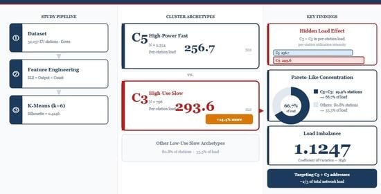
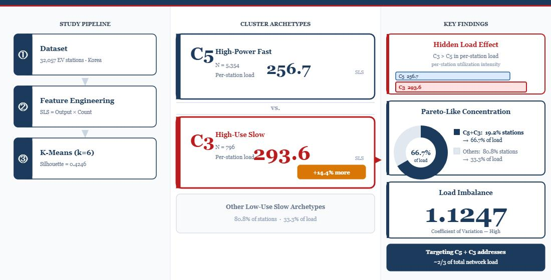
This study has notable contributions, including: (i) identification of six distinct behavioral archetypes of EV charging stations through unsupervised clustering; (ii) characterization of HLE showing that high-frequency slow-charging stations can cause more stress to the grid on a per-station basis than does high-power fast-charging stations; (iii) discovery of a highly concentrated load distribution pattern where only 19.2% of stations account for approximately 66.7% of the total grid load; and (iv) feature importance analysis based on SHAP indicating a dominant influence from geographic and infrastructure-related attributes in terms of cluster discrimination.

2. Literature Review

The use of machine learning in electric vehicle charging infrastructure has advanced along two mostly parallel paths: demand forecasting and spatial planning. Nazari et al. [6] reported in detail on clustering techniques designed for electric vehicles and used either hard or soft methods as two key methodologies to alleviate the computational burden and model the behavioral complexity of large EV populations that are integrated into distribution networks. They found that K-Means and hierarchical approaches dominate the academic literature on EV clustering, but cited a lack of applications to characterize stations as load-bearing infrastructure archetypes, as most focus on user behavior segmentation or charging station siting.

The complementary body of literature addresses the modeling of individual EV user charging behavior. Shahriar et al. [7] carried out a systematic review of ML approaches for EV charging behavior prediction, reviewing session duration, energy demand, departure time, and frequency estimation. They show that ensemble techniques in general, and Random Forest and XGBoost specifically, consistently outperform individual models on behavioral prediction tasks, and also that contextual variables such as traffic conditions, weather, and time of day increase precision significantly. These findings are directly relevant to infrastructure characterization, as session frequency and duration patterns determine whether a station operates predominantly in slow-charging, fast-charging, or high-frequency slow-charging regimes, which are the key distinctions examined in this study.

Recent years have seen a growing interest in applying SHAP to EV charging systems. Ullah et al. [8] employed an XGBoost classifier with SHAP analysis to predict charging station choice behavior, demonstrating the main decision factors for EV users in selecting a given charging station: location, availability (opened), pricing, and type of station. Their research put a methodological blueprint into place for interpretable machine learning on the EV. Integrating ensemble classifiers with a SHAP-based post hoc explanation allows practitioners to discover which underlying characteristics of their infrastructure exhibited the strongest influence on observable behavioral patterns. This study builds on that approach at the user decision level to the infrastructure archetype level, using SHAP to reveal which station features have the most strongly determining cluster membership with respect to the six behavioral archetypes identified.

A new research stream on optimizing charging station locations has developed, usurping many heuristic approaches with data-driven methods. Magsino et al. [9] used K-Means and density-based clustering methods on GPS mobility traces from taxi and ride-hailing fleets in Singapore, Jakarta, and another Southeast Asian city to show that origin-destination trajectory analysis yields station placement recommendations closely correlated with empirically observed demand concentrations. Li et al. [10] employed more advanced techniques such as multi-type clustering and grid-based aggregation of demand to gather reservation patterns through the usage of taxi GPS paths in Qingdao, China, addressing optimal locations for charging stations while minimizing the travel distance on average, while satisfying station satisfaction conditions. These trajectory-based strategies illuminate not just where drivers go, but also where they linger long enough to allow charging, tapping a behavioral cadence that purely geographic or demand-density approaches cannot deliver. Collectively, these studies establish GPS mobility data as a usable input for charging infrastructure spatial planning and motivate the missing elements of station-level behavioral archetypes that mediate between spatial planning and the characterization of load.

Korea’s EV charging ecosystem features a unique institutional environment. Kim et al. [11] performed an economic feasibility analysis of public charging infrastructure in Korea and its evolution from free public charging (2011–2016) to metered pricing regimes, showing that an investment in charging infrastructure is more cost-effective for battery electric vehicle adoption than the purchase subsidies. In a companion spatial study, Kim and Kim [12] investigate the factors determining public fast-charging station locations across the Seoul Metropolitan Area and find a negative correlation between traffic volume and station location. This counterintuitive finding indicates that demands for siting have been driven more by administrative and property-availability considerations than through systematic demand analysis. These findings indicate that there is a structural misalignment between the logic used to deploy infrastructure and real-world patterns of demand for behavior, providing direct policy relevance for the station-level archetype characterization approach we pursue in this study.

Fescioglu-Unver and Yıldız Aktaş [13] provided a thorough review of the wide variety of studies on machine learning applications in EV charging, ranging from infrastructural planning to charge scheduling to dynamic pricing to vehicle routing. In particular, their analysis finds the three dominant methodological families in the field to be forecasting, clustering, and reinforcement learning, which determines that customer concerns, especially availability, reliability, and wait time, are first-order drivers of EV adoption rates. Also, if the adoption process is archetype-based, then infrastructure planning that does not account for station behavioral heterogeneity will miss one of the strongest levers to increase market penetration.

Clustering has been utilized for location selection as well as load forecasting on the station level. Moving on to location planning, techniques utilizing GPS mobility traces have shown that the placement of charging stations using clusters leads to a better correlation with actual demand rather than heuristics. To append for load forecasting, deep learning-based spectral clustering is utilized to deal with statistical heterogeneity in regional EV charging loads so that global forecasting models are not applicable, as regional charging loads exhibit statistically heterogeneous distributional profiles [14]. Moreover, behavioral clustering of fast-charging sessions has also been investigated using agglomerative methods, with distinct usage patterns identified at highway stations [15]. At the feeder level, clustering using K-Means on representative distribution circuits has facilitated a systematic evaluation of smart-charging strategies [16], with the results highlighting that behavioral characterization is a key precursor to successful upgrade planning at high EV penetration. Smart-charging demand response research further demonstrates that load-shifting strategies are most successful when grouped by behavioral archetypes, as opposed to treating stations as a homogenous pool. Yet the combination of heterogeneous station types and cumulative grid load concentration has yet to be formally modeled. Most demand forecasting studies implicitly assume that high-power fast charging will be the primary source of grid stress, neglecting to consider how a large fleet of high-frequency slow-charging stations can also impact grid stability. It is this gap that motivates the HLE concept introduced in this work.

The rich literature pertaining to grid integration and vehicle to grid (V2G) identifies the wealth of actionable station-level behavioral intelligence. Jenn and Highleyman [17] utilized real-world PG&E’s feeder circuit data together with census-block-level EV adoption estimates to analyze projections of future distribution loading in Northern California, resulting in their estimate that, under a six million EV adoption scenario, circa 20% of distribution feeders need upgrades. Their analysis categorized commercial versus residential feeder stress profiles, revealing that feeder-level behavioral heterogeneity, rather than aggregate EV penetration alone, determines where infrastructure stress concentrates. Nutkani et al. [18] investigated the mechanisms employed in the uncontrolled EV charging that result in transformer overload, voltage imbalance, and harmonic distortion of distribution networks, identifying demand-side segmentation as a prerequisite for effective mitigation strategies. Expanding on this foundation, Zhang et al. [19] proposed a large-scale V2G scheduling algorithm based on the alternating direction method of multipliers (ADMM), demonstrating that coordinated management of aggregated charging and discharging can achieve simultaneous peak load reduction and reactive power compensation. Their framework explicitly requires feeder-level and station-type characterization as inputs in its hierarchical optimization structure. Collectively, these studies lead to an infrastructure planning paradigm that functions at the station-archetype scale, which is precisely the contribution of the CLC and load imbalance coefficient of variation metrics proposed here.

The dataset for this study was created and published by Seo, Moon and Kwon [4], with the purpose of developing a graph neural network-based charging station recommendation system tailored for the Korean EV market. The publicly available dataset [5] is the largest simulation of EV driver–station interaction in Korea, which can be used for characterizing load at an infrastructural level and serves as a supporting contribution to the primary recommendation goal.

All machine learning implementations are based on well-known approaches: K-Means with k-means++ initialization [20], Decision Tree [21], Logistic Regression [22], Random Forest [23], and XGBoost, which is a gradient-boosting framework for trees [24]. To assess cluster validation, this study adopted the Elbow method [20], use of the Silhouette coefficient [25], and Davies–Bouldin Index [26]; to explore model interpretability, SHAP was used [3].

The analytical pipeline presented in this study is intentionally built on interpretable traditional machine learning methods. Deep learning clustering approaches, while powerful in high-dimensional temporal domains, require session-level timestamp data to capture spatiotemporal correlations meaningfully, data that are not available in this dataset. The seven-feature station-level input space is well-suited to K-Means with k-means++ initialization, which offers deterministic convergence, validated stability across initializations, and direct SHAP-based interpretability of cluster membership drivers. Applying sequence-based architectures (e.g., LSTM, Transformer) to aggregate station-level features without temporal resolution would introduce false structural assumptions and reduce interpretability without providing meaningful gains for the archetype discovery objective.

3. Materials and Methods

3.1. Dataset

This study utilizes the publicly available dataset published by Seo, Moon and Kwon [4] and deposited on Mendeley Data [5], which consists of records for 32,057 EV charging stations and 667,210 simulated driver interactions across the Republic of Korea. The station metadata file includes 25 features per station, such as geographic coordinates (latitude, longitude), administrative region codes, charger type, output capacity (kW), charging speed classification, and operator identifiers. All analyses were conducted in Python 3.10.0 (Google Colab, Google LLC, Mountain View, CA, USA) using the following libraries: scikit-learn 1.6.1, XGBoost 3.2.0, SHAP 0.51.0, pandas 2.2.2, NumPy 2.0.2, SciPy 1.16.3, matplotlib 3.10.0, and seaborn 0.13.2.

3.2. Feature Engineering

Seven features were chosen to be clustered and classified: output capacity (kW), session count (count), fast or slow flag (is_fast), code of the type of charger (chgertype), latitude and longitude of the station, and a regional code (zcode).

StandardScaler was used on continuous features to remove scale differences in variables with heterogeneous units and ranges to guarantee numerical stability in distance-based or model-based learning algorithms. A composite load proxy was developed to approximate the total load imposed by each charging station, called the station load score (SLS), which jointly captures both its power capacity and usage intensity. Equation (1) defines the SLS:

$$\mathrm{S}\mathrm{L}\mathrm{S}=\mathrm{o}\mathrm{u}\mathrm{t}\mathrm{p}\mathrm{u}\mathrm{t}\left(\mathrm{k}\mathrm{W}\right)\times \mathrm{C}\mathrm{o}\mathrm{u}\mathrm{n}\mathrm{t}$$

(1)

The SLS represents a relative utilization intensity proxy that jointly captures installed power capacity and session frequency. Not only does it not directly measure actual energy demand or instantaneous grid stress, but data on the duration of sessions is unavailable; however, stations with an identical SLS value may have a completely different impact on the grid depending on whether the sessions there are temporally concentrated or spread across the day.

It is important to emphasize that the SLS is a dimensionless relative proxy and does not represent actual energy delivered (kWh) or instantaneous grid stress. Session duration data are unavailable in this dataset; stations with identical SLS values may impose substantially different peak load profiles depending on the temporal concentration of their charging sessions. All load-related findings in this study, including the hidden load effect, are accordingly interpreted under this proxy assumption and should be validated against real session-duration data in future work.

3.3. Clustering

To identify behavioral archetypes, we applied K-Means clustering with k-means++ initialization [20]. The best clusters were identified with the Elbow method and inertia, using the Silhouette coefficient [25], and the Davies–Bouldin Index (DBI) [26] for k values between 2 and 10.

To guarantee the stability of solutions, K-Means configurations were compared with $init\in \{k-means++,random\}$ and $n_{init}\in \{5,10,20,30\}$ after the optimal number of clusters was determined. Four different linkage methods (ward, complete, average, single) and three distance metrics (Euclidean, cityblock, cosine) were tested as an alternative approach with agglomerative clustering. All clustering inputs were first standardized with StandardScaler [27] before analysis.

The stability assessment confirmed that cluster assignments, archetype profiles, and load/station values remained consistent across all tested K-Means configurations. The k-means++ initialization method inherently reduces sensitivity to random seed selection relative to random initialization, further ensuring the reproducibility of the k = 6 solution reported in this study.

3.4. Supervised Classification

The supervised classification stage serves a dual purpose. First, it functions as a cluster separability validation procedure: by demonstrating that structurally distinct classifiers can reliably recover cluster assignments from the same feature space with high F1 macro and ROC-AUC, we confirm that the six K-Means archetypes are geometrically well-separated and internally consistent. Near-perfect classification performance is both expected and desirable as evidence of meaningful, stable cluster partitions and does not constitute data leakage. Second, the trained classifiers provide deployment utility: a new charging station with known feature values can be assigned to one of the six behavioral archetypes without re-running K-Means. The train/test split (80:20, stratified, random_state = 42) and a StandardScaler fitted exclusively on training data ensure that no test-set information contaminates model training or evaluation.

We trained four classifiers on the generated K-Means cluster labels: Decision Tree [21], Logistic Regression [22], Random Forest [23], and XGBoost [24]. They were chosen to represent linear and nonlinear decision boundaries and ensemble-based learning approaches, respectively.

The feature matrix used for classification was constructed with the same seven variables that were used in clustering. Stratified sampling for splitting the data into training and test was used with an 80:20 split (with random_state = 42). For models that needed inputs to be scaled, a StandardScaler was fit on the training data and then applied to the test data. Logistic Regression and Decision Tree were trained on scaled features, while Random Forest and XGBoost were trained on the original feature space.

Hyperparameter optimization was performed using RandomizedSearchCV (n_iter = 50, five-fold cross-validation, random_state = 42 and the primary scoring metric was F1 macro [27]). For each classifier, model-specific parameter distributions were defined separately.

The performance of the final model was evaluated on the held-out test set using accuracy, precision (macro), recall (macro), F1 (macro) [28], Matthews correlation coefficient (MCC) [29,30], and ROC-AUC (macro, One-vs-Rest) [31].

3.5. SHAP Interpretability

SHAP (SHapley Additive exPlanations) was applied to the best classifier automatically selected based on the F1 macro score in the held-out test set, using Matthews correlation coefficient (MCC) as a tie-breaking criterion. In the case of tree-based models (Decision Tree, Random Forest, XGBoost), TreeExplainer [3] was used, while in Logistic Regression, LinearExplainer was applied instead. In this study, Random Forest achieved the highest F1 macro and was therefore selected as the SHAP model. SHAP values were calculated on the test set, producing a three-dimensional output array with dimensions (samples, features, classes). In the case of sklearn-based models, which return a list of per-class arrays, the output was normalized to a common format by array stacking. Mean absolute SHAP values over all samples and classes were calculated for global feature importance, while per-cluster importance was obtained individually for each archetype to understand which features most strongly determine cluster membership.

3.6. Grid Load Distribution and Cluster-Level Metrics

Three metrics were introduced to characterize load distribution across cluster archetypes.

The CLC of cluster $k$ is defined in Equation (2):

$${\mathrm{C}\mathrm{L}\mathrm{C}}_k= {\displaystyle \frac{\sum {\mathrm{S}\mathrm{L}\mathrm{S}}_k}{\sum {\mathrm{S}\mathrm{L}\mathrm{S}}_{\mathrm{t}\mathrm{o}\mathrm{t}\mathrm{a}\mathrm{l}}}}$$

(2)

where $\sum {\mathrm{S}\mathrm{L}\mathrm{S}}_k$ is the station load score of cluster $k$, and $\sum {\mathrm{S}\mathrm{L}\mathrm{S}}_{\mathrm{t}\mathrm{o}\mathrm{t}\mathrm{a}\mathrm{l}}$ is the total load across all clusters.

Equation (3) defines the load imbalance coefficient of variation (CV).

$$\mathrm{C}\mathrm{V}={\displaystyle \frac{{\sigma }_{\mathrm{C}\mathrm{L}\mathrm{C}}}{{\mu }_{\mathrm{C}\mathrm{L}\mathrm{C}}}}$$

(3)

where ${\sigma }_{CLC}$ and ${\mu }_{CLC}$ are the standard deviation and mean of cluster-level load contributions.

We define the hidden load effect (HLE) as the difference in average load per station between high-use slow (C3) and high-power fast (C5) clusters, according to Equation (4):

$$\mathrm{H}\mathrm{L}\mathrm{E}={\displaystyle \frac{\sum {\mathrm{S}\mathrm{L}\mathrm{S}}_{\mathrm{C}3}}{{\mathrm{N}}_{\mathrm{C}3}}}-{\displaystyle \frac{\sum {\mathrm{S}\mathrm{L}\mathrm{S}}_{\mathrm{C}5}}{{\mathrm{N}}_{\mathrm{C}5}}}$$

(4)

where SLS is the station load score and $N$ is the number of stations within each cluster.

Moreover, a relative form of the hidden load effect is given by Equation (5):

$${\mathrm{H}\mathrm{L}\mathrm{E}}_{\mathrm{r}\mathrm{e}\mathrm{l}}={\displaystyle \frac{\frac{\sum {\mathrm{S}\mathrm{L}\mathrm{S}}_{\mathrm{C}3}}{N_{\mathrm{C}3}}-\frac{\sum {\mathrm{S}\mathrm{L}\mathrm{S}}_{\mathrm{C}5}}{N_{\mathrm{C}5}}}{\frac{\sum {\mathrm{S}\mathrm{L}\mathrm{S}}_{\mathrm{C}5}}{N_{\mathrm{C}5}}}}$$

(5)

In the absolute hidden load effect (HLE, Equation (4)) and in relative form (${\mathrm{H}\mathrm{L}\mathrm{E}}_{\mathrm{r}\mathrm{e}\mathrm{l}}$, Equation (5)), we express the difference in mean SLS per station as: (i) a simple difference, (ii) a percent of C5’s mean SLS. Distinct feature distributions dictated the cluster archetypes. The high-power fast cluster corresponds to stations with a fast_ratio greater than 0.9, while the high-use slow cluster corresponds to stations with a fast_ratio less than 0.1 and the highest mean session count.

4. Results

4.1. Exploratory Data Analysis

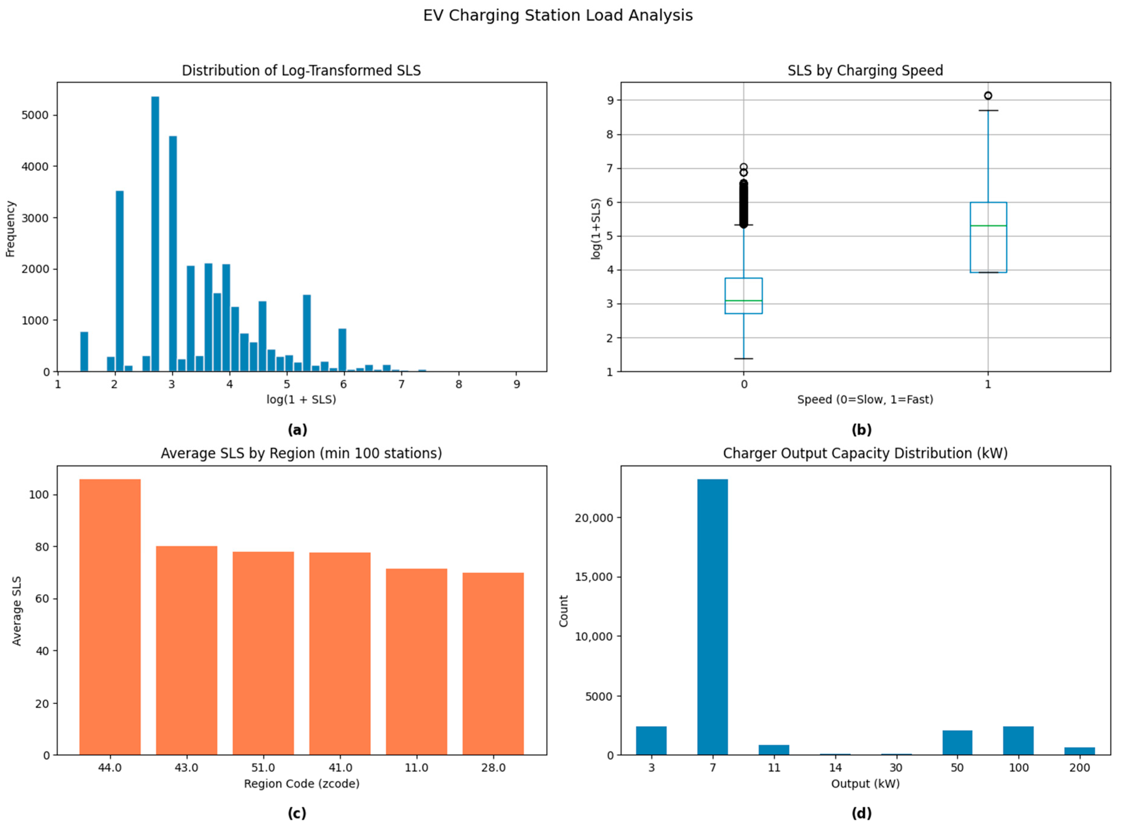
The data set contains 32,057 charging stations, including 5345 (16.7%) fast chargers and 26,712 (83.3%) slow chargers. The distribution of the SLS is highly right-skewed (mean = 75.2, max = 9360), indicating that a small subset of stations carries disproportionately higher shares of cumulative load compared to others. The log-transformed distribution of the SLS (as exemplified in Figure 1) illustrates this skewness even better. Fast chargers were linked to significantly higher SLS values than slow chargers; this trend was confirmed by the boxplot showing a higher median for fast chargers compared to slow ones and increased dispersion.

There is considerable geographic heterogeneity in these regional analyses. For the regions with more than 100 stations, region 44 has the highest SLS average and is followed by regions 43, 51, and 41, while lower SLS averages were observed in regions 11 and 28 (Figure 1). An additional pattern is clearly observable when comparing the charger capacities, which highlights that some output levels (7 kW and higher-capacity chargers, e.g., 50 kW and 100 kW) are occurring more frequently than others, indicating a non-uniform distribution of charging infrastructure across capacity.

4.2. Clustering Results

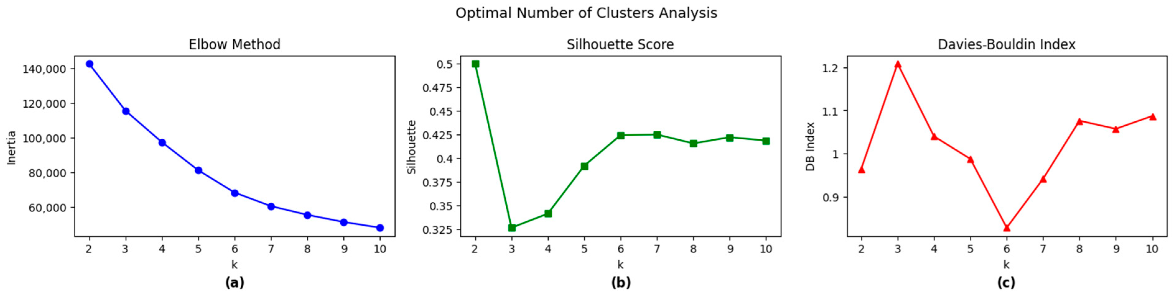
The Elbow, Silhouette, and Davies–Bouldin (DBI) analyses for k = 2 to 10 are shown in Figure 2.

Table 1. Silhouette score and Davies–Bouldin Index (DBI) for k = 2 to 10.

k	Silhouette	DBI	Note
2	0.5001	0.9642	Silhouette maximum
3	0.3267	1.2085
4	0.3416	1.0398
5	0.3922	0.9874
6	0.4245	0.8277	DBI minimum—selected
7	0.4252	0.9412	Silhouette secondary peak
8	0.4158	1.0760
9	0.4223	1.0571
10	0.4188	1.0869

presents the Exact Silhouette and DBI scores for each k. The Silhouette score is maximized at k = 2 (0.5001), indicating the disproportionately strong binary separation of fast and slow chargers, a structure already present in the is_fast feature, and known a priori from dataset metadata. A selection of k = 2 would thus retrieve an existing label rather than illuminating latent behavioral structure. After k = 2, the Silhouette score drops down more rapidly to k = 3 (0.3267) and recovers to a second plateau at k = 6–7. Crucially, k = 7 produces a marginally higher Silhouette score than k = 6 (0.4252 vs. 0.4245, difference of 0.0007) and by contrast a substantially worse DBI (0.9412 vs. 0.8277). Thus, the choice of k = 6 is validated by the minimum in DBI, the Elbow inflection point, and interpretability considerations, with an additional validation based on the Silhouette criterion, which is to be considered as a secondary indicator due to its sensitivity to pre-existing binary structure.

After trying different linkage and distance combinations, it appears single linkage on cityblock produces a particularly high Silhouette score, but comes at the cost of quite extreme imbalance within clusters in terms of sizes, leading to a chaining effect. Euclidean distance linkage by Ward proved to form better-connected structures but resulted in overall clusters of not greater compactness and separation than K-Means. Thus, K-Means was chosen as the main clustering algorithm.

Table 2. K-Means cluster behavioral profiles (k = 6).

Cluster	N	Fast Ratio	Mean Output (kW)	Mean Count	Load/Station *	Archetype
C0	3408	0.00	7.03	4.48	31.5	Low-Use Slow (W)
C1	6713	0.00	7.24	4.62	33.0	Low-Use Slow (N)
C2	7990	0.00	6.96	4.50	31.3	Low-Use Slow (C)
C3	796	0.01	6.68	44.08	293.6	High-Use Slow
C4	7796	0.00	6.75	4.42	28.9	Low-Use Slow (S)
C5	5354	0.99	97.80	2.33	256.7	High-Power Fast

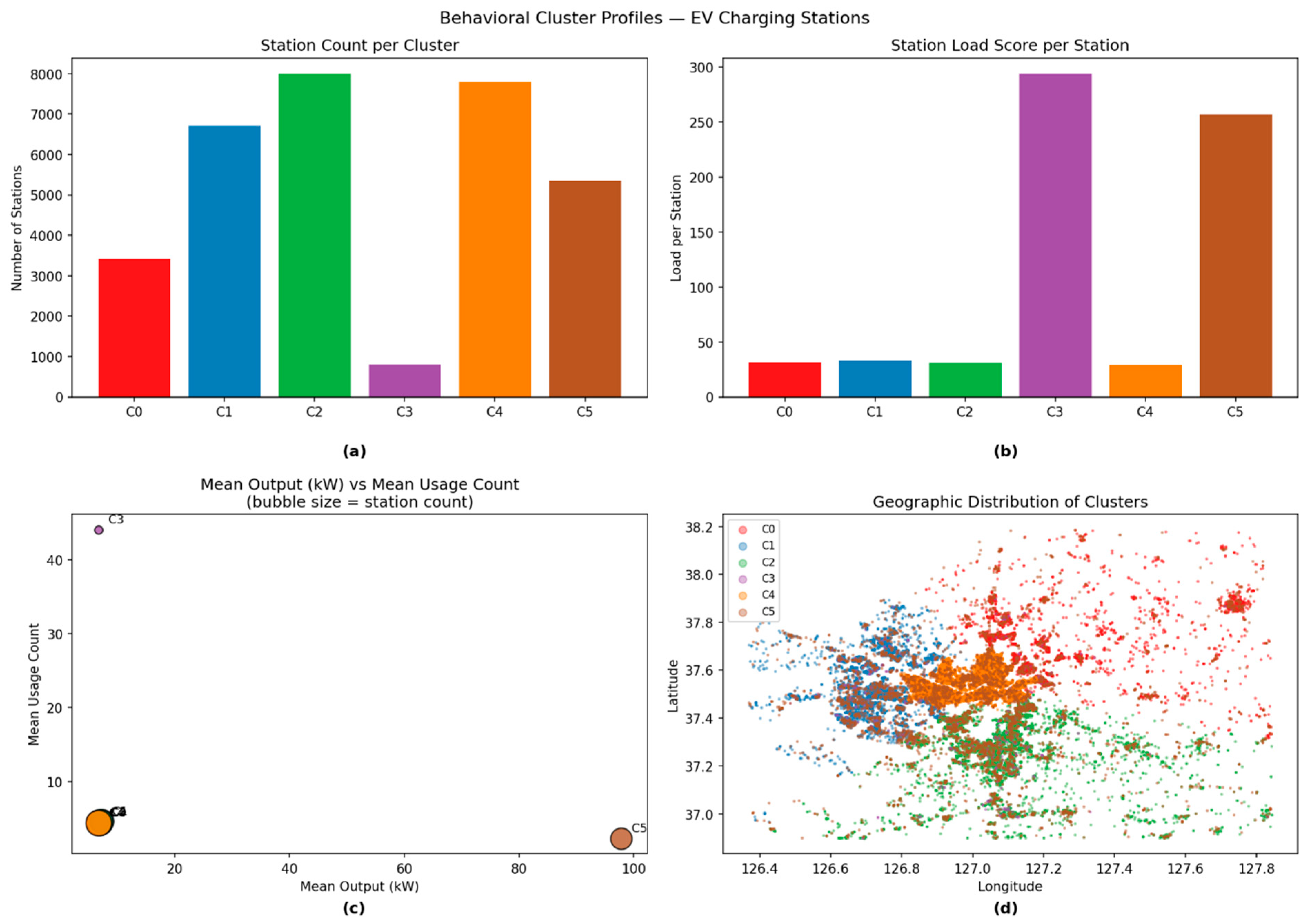
* load/station = total SLS ÷ station count.

summarizes and Figure 3 visualizes the six K-Means cluster behavioral profiles. Cluster C5 is defined by high-power charging stations, where the average output levels are significantly higher than those of other clusters. Cluster C3 has significantly higher loads per station, suggesting a notable degree of use, despite relatively low power levels. In contrast, clusters C0, C1, C2, and C4 all share a similar low-usage, low-output profile; the difference among them lies mainly in their spatial distribution (See Figure 3). This resulted in four low-use slow sub-clusters, labeled W, N, C, and S for approximate relative spatial tendencies; however, there was considerable geographic overlap between these groups. The operational profiles of these four clusters are very similar (load/station range: 28.9–33.0), and they differ mainly based on the spatial location rather than behavioral insights. From a grid planning standpoint, however, these sub-cluster groups can be merged into a single low-use slow archetype with no loss of operationally relevant information; the fact that they appear as separate clusters in the k = 6 solution derives from geographic heterogeneity captured by the dataset rather than meaningful operational differentiation, corroborated by further examination through SHAP as seen in Section 4.4.

From a grid load management perspective, the four low-use slow sub-clusters (C0, C1, C2, C4) can be consolidated into a single low-use slow archetype without any operational information loss, yielding a simplified three-archetype representation: low-use slow (consolidated), high-use slow (C3), and high-power fast (C5). This consolidated framework is recommended for practitioners focused on demand-side management and infrastructure prioritization, where the operationally critical distinction lies between C3 and C5 rather than among the geographically differentiated low-use slow sub-clusters.

4.3. Classification Results

The supervised classification stage is designed as a cluster separability validation procedure. Near-perfect F1 macro and ROC-AUC values confirm that the six behavioral archetypes are geometrically well-separated in the feature space, which is both the intended and expected outcome of this validation design.

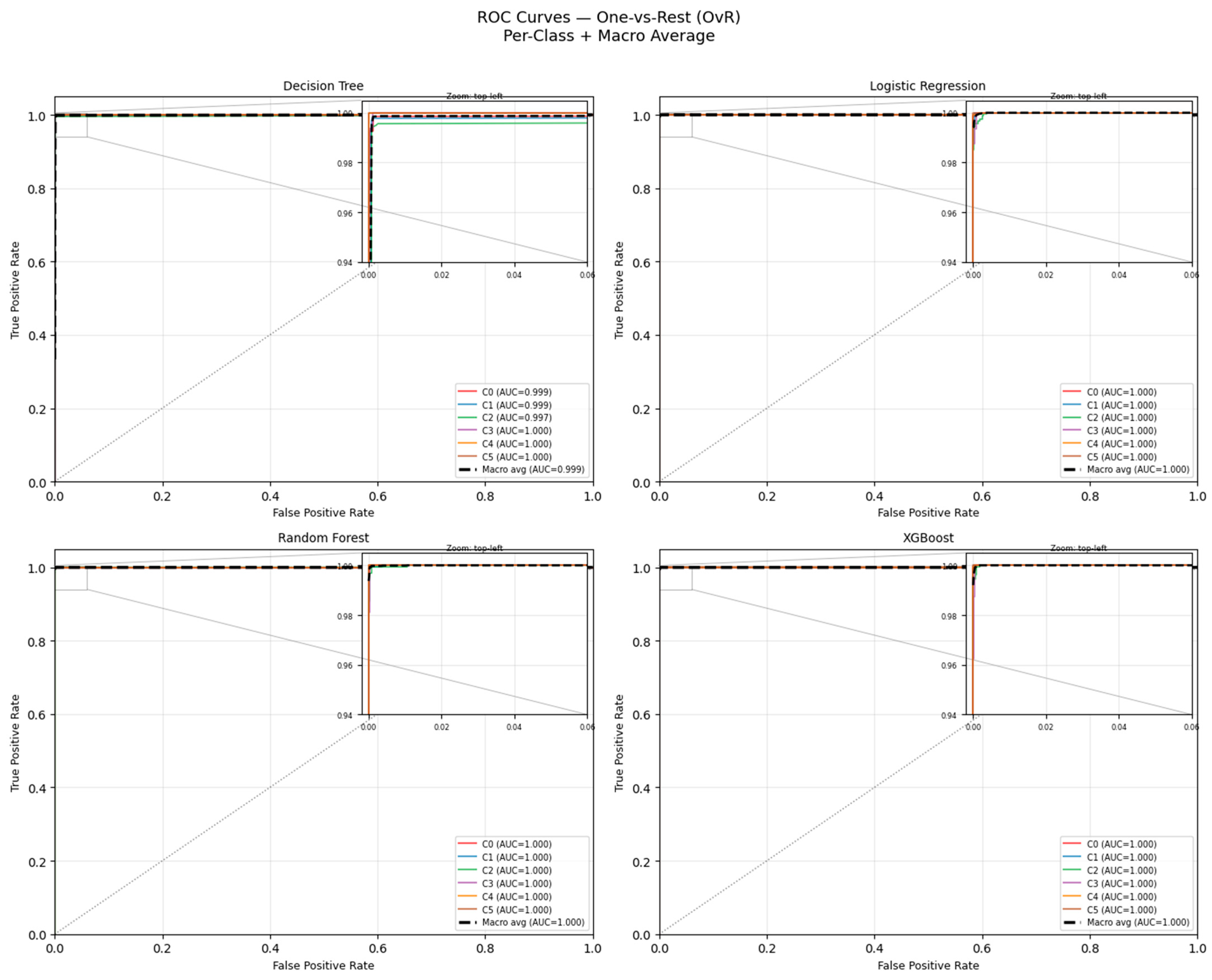
As shown in

Table 3. Classification performance on held-out test set (optimized models).

Model	Accuracy	Precision	Recall	F1 Macro	MCC	AUC	CV F1
Decision Tree	0.9970	0.9911	0.9972	0.9941	0.9963	0.9992	0.9930
Logistic Regression	0.9978	0.9961	0.9966	0.9964	0.9973	1.0000	0.9975
Random Forest	0.9988	0.9971	0.9981	0.9976	0.9984	1.0000	0.9956
XGBoost	0.9983	0.9966	0.9977	0.9972	0.9978	1.0000	0.9955

MCC = Matthews correlation coefficient; AUC = ROC-AUC macro (OvR); CV F1 = RandomizedSearchCV best_score_.

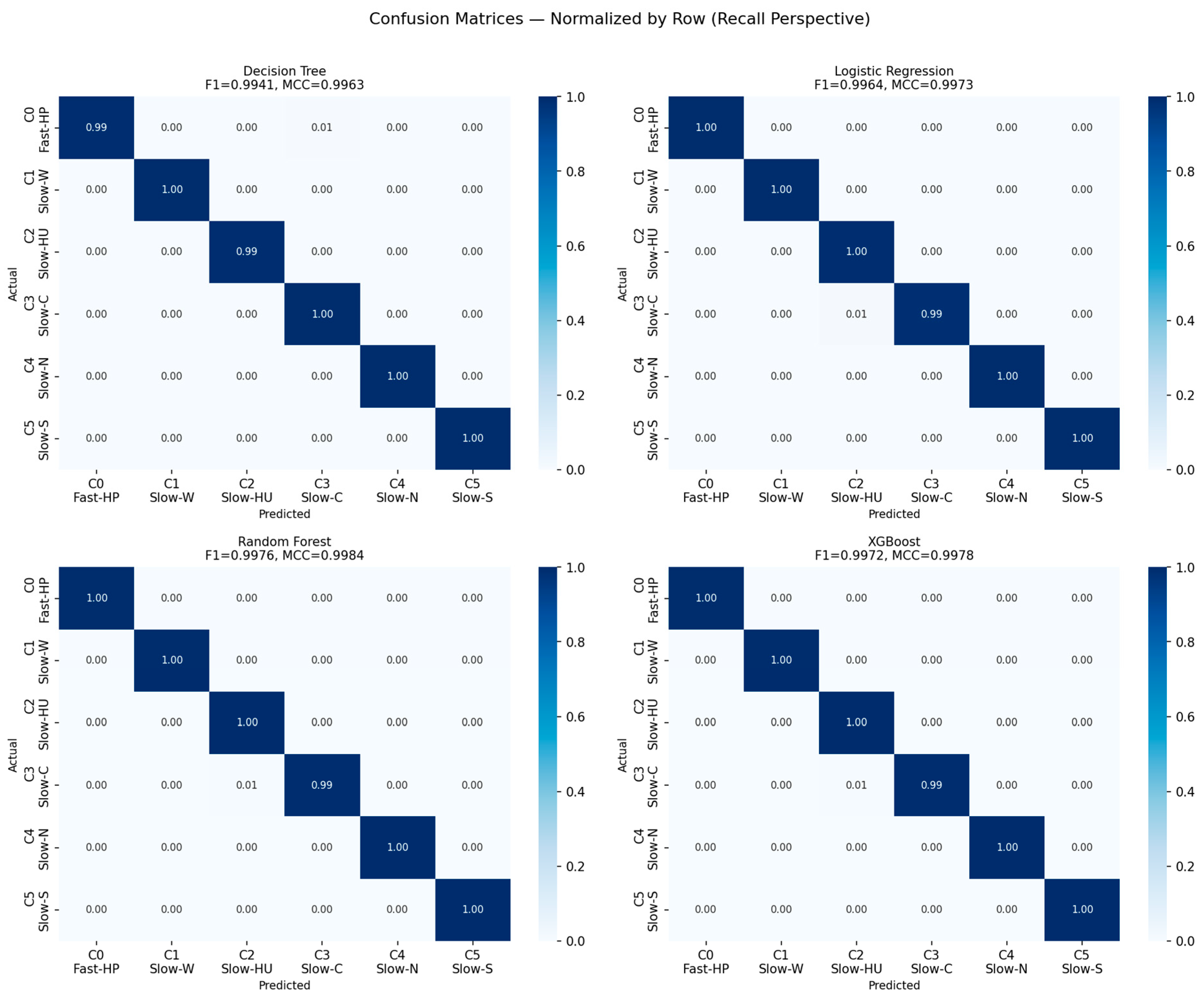
, with accompanying visualizations in Figure 4 and Figure 5, all four classifiers achieved near-perfect performance on the held-out test set. Among the models, Random Forest produced the best overall performance on most evaluation metrics, closely followed by XGBoost, Logistic Regression, and Decision Tree. All models obtained accuracy, F1 macro, and MCC measures > 0.99, indicating highly consistent classification capability across cluster labels, with marginal performance differences between models. Cross-validation results obtained via RandomizedSearchCV are closely aligned with test set performance, suggesting stable generalization and no apparent overfitting.

Finally, the normalized confusion matrices in Figure 4 reveal near-perfect classification performance across all clusters, with most predictions falling along the diagonal. Minor misclassifications can be found, especially for cluster C3, where a small proportion of samples were confused with other slow-charging clusters. This is consistent across models, as the structure of these clusters with respect to their charging behavior is also comparable.

The ROC curves shown in Figure 5 were nearly perfectly separable for all classes. The class-wise curves are close to the top-left corner of the plot, showing very high true positive rates with almost no false positive rates. Values for the macro-average AUC were all ~1.00 across all models, reflecting the strong discriminative power of the feature space.

4.4. SHAP Feature Importance

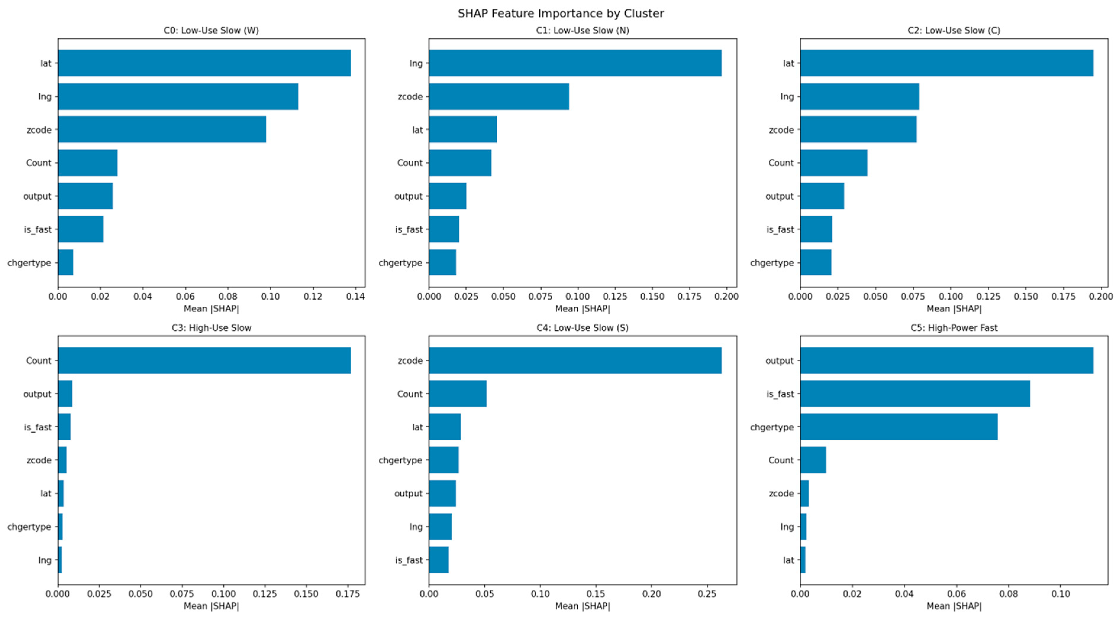
The per-cluster SHAP analysis in Figure 6 shows that feature dominance varies between cluster archetypes. In the case of cluster C5 (high-power fast), features related to output capacity appear as the most significant, in addition to binary variables describing a fast-charger (is_fast) and charger type itself, which reflects its association with high-power charging infrastructure. For cluster C3 (high-use slow), session count is clearly the dominant feature, with a wide separation of high-usage stations from all other clusters. The presence of location variables, specifically latitude, longitude, and zcode, as the most important variable for clusters C0, C1, C2, and C4, suggests that these clusters are predominantly spatially distinct from operational characteristics.

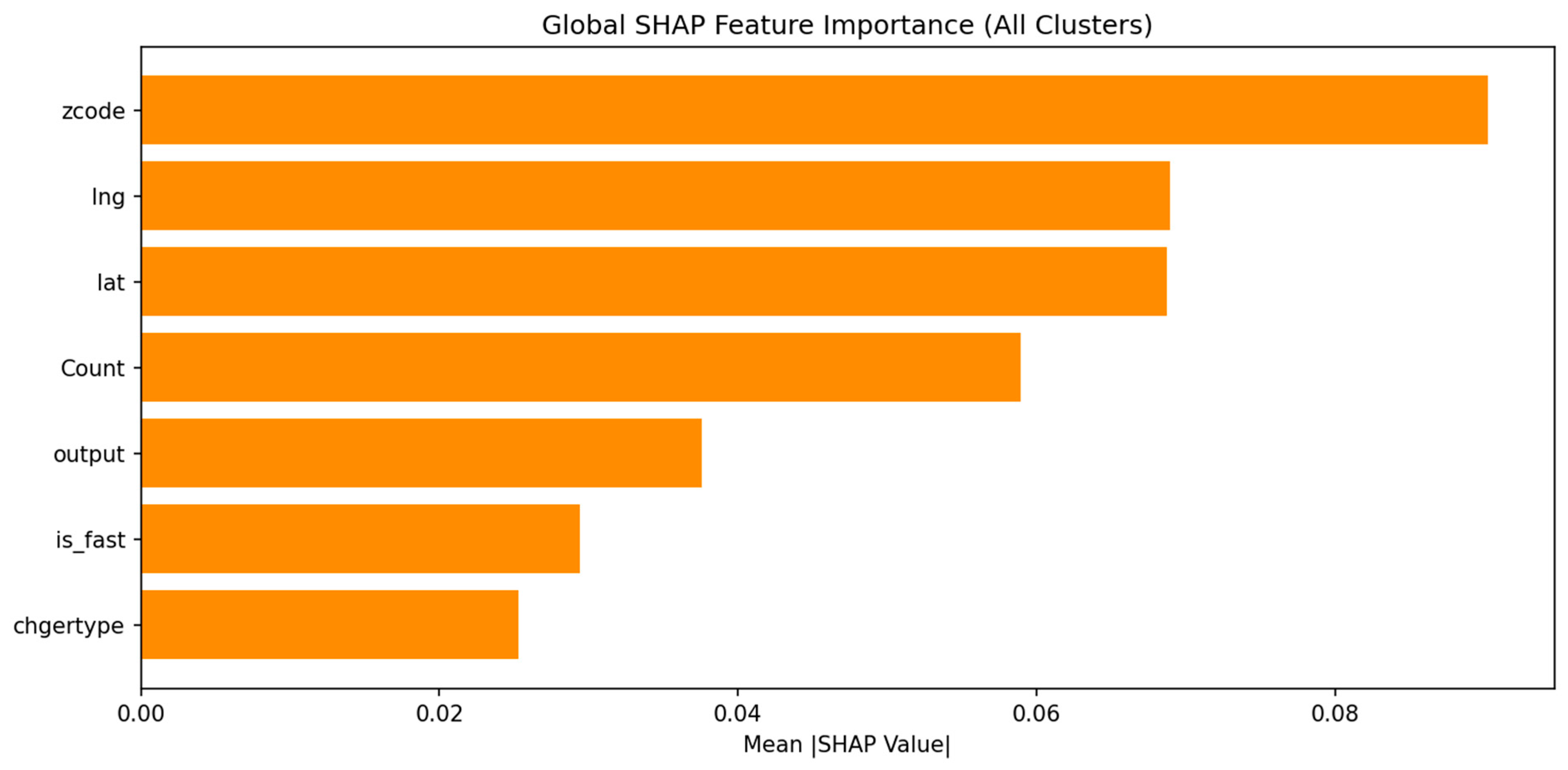
In line with these cluster-specific trends, the global SHAP analysis shows that overall, regional encoding (zcode) is by far the most important single variable, followed closely by longitude and latitude (in Figure 7). Usage intensity (session count) ranks fourth, and output capacity and charger type play a moderate role. Meanwhile, the is_fast binary fast-charger indicator had the lowest global importance. This indicates that charging speed classification alone carries limited discriminative power when spatial and usage-intensity features are present. An important general observation, however, is that the four low-use slow clusters (C0, C1, C2, C4) dominate in terms of their global SHAP ranking, and together accounting for 80.8% of all stations, are primarily differentiated by geographic variables. For the two operationally critical archetypes, C3 (high-use slow) and C5 (high-power fast), geographical features are much less important than their operational counterparts: session count is the decisive feature for C3, while output capacity, is_fast, and charger type are all highly predictive of C5. Infrastructure planners should thus interpret the global SHAP ranking cautiously; per-cluster importance profiles provide more actionable guidance for the prioritization of demand-side management and grid upgrades.

The dominance of geographic variables (zcode, latitude, longitude) in SHAP-based cluster discrimination does not necessarily imply that the clustering captures geography alone rather than operational behavior. In EV charging ecosystems, spatial variables frequently encode latent infrastructural and demand-related characteristics, including urban density, charger deployment policies, regional mobility demand, land-use structure, and accessibility constraints. Geographic differentiation may therefore function as an indirect representation of heterogeneous charging demand environments. Importantly, the two operationally critical archetypes, C3 (high-use slow) and C5 (high-power fast), remain primarily driven by infrastructure utilization variables rather than geographic encoding.

Two interpretive frames should be distinguished when applying SHAP findings in practice. In the spatial differentiation frame, geographic variables (zcode, longitude, latitude) dominate global SHAP importance because 80.8% of stations belong to low-use slow clusters that are operationally equivalent but geographically dispersed; this insight is relevant for infrastructure siting and regional deployment planning. In the grid-load behavior frame, operational features dominate for the two critical archetypes: session count is the decisive feature for C3 (high-use slow), while output capacity, is_fast, and charger type are most predictive for C5 (high-power fast). Infrastructure planners focused on demand-side management and load prioritization should therefore consult per-cluster SHAP profiles rather than the global SHAP ranking, which is dominated by the geographically differentiated majority.

4.5. Implications of Grid Load Concentration and the Hidden Load Effect

The CLC for all six archetypes is displayed in

Table 4. CLC analysis.

Cluster	N	CLC (%)	Load/Station	Load/1000 *	Archetype
C0	3408	4.45	31.5	1.31	Low-Use Slow (W)
C1	6713	9.19	33.0	1.37	Low-Use Slow (N)
C2	7990	10.36	31.3	1.30	Low-Use Slow (C)
C3	796	9.69	293.6	12.17	High-Use Slow
C4	7796	9.34	28.9	1.20	Low-Use Slow (S)
C5	5354	56.97	256.7	10.64	High-Power Fast

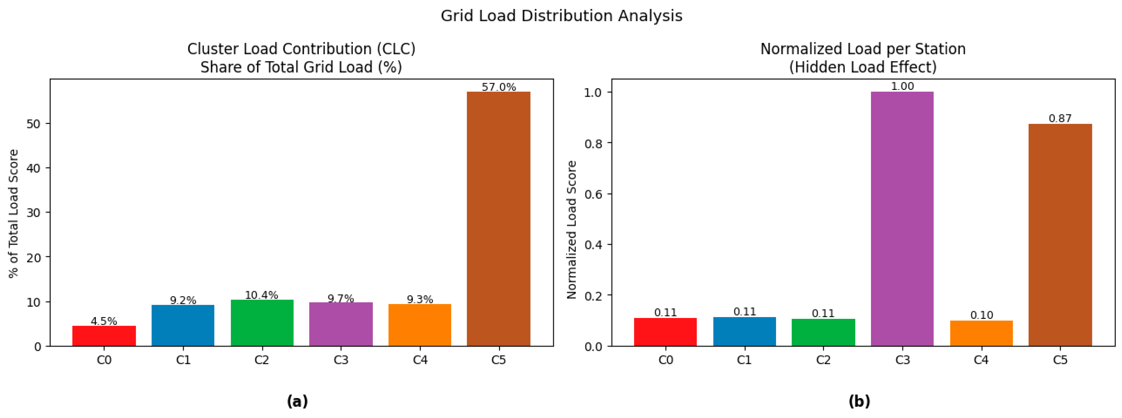
* load/1000 = CLC(%) ÷ N × 1000, indicating SLS-based load contribution per 1000 stations.

and visualized by the results seen in Figure 8. Cluster C5 (high-power fast) makes up about 57% of the total SLS-based network load, while the cluster constitutes approximately 16.7% of all stations. Cluster C3 (high-use slow) comprises only a small fraction of the network, yet contributed nearly 9.7% of the total SLS-based load. The joint weight of clusters C5 and C3 makes up less than 1/5 of all stations but almost 2/3 of the total SLS-based network load, showing a high concentration in the space utilization distribution.

A relatively high load imbalance coefficient of variation (1.1247) indicates that SLS-based load contributions across clusters exhibit a significant degree of variance, endorsing the existence of this trend.

The load-per-station comparison normalized by SLS (Figure 8) indicates a notable pattern. Cluster C3 exhibits a higher SLS-based load per station than cluster C5, despite consisting primarily of slow chargers. This finding suggests that usage intensity, rather than charging speed alone, plays a critical role in determining per-station utilization intensity. However, this directionality assumes comparable mean session durations across archetypes; if fast-charging sessions in C5 are systematically shorter than slow-charging sessions in C3, actual energy delivery per station in C5 may exceed that implied by the SLS proxy alone.

5. Discussion

The six cluster archetypes found in this study align with behavioral heterogeneity expressed in previous EV clustering studies [6,14,15]. The delineated nature of C5 (high-power fast) and C3 (high-use slow) as operationally distinct archetypes suggests that charging speed and usage intensity can be treated in a largely independent fashion, with respect to the behavioral dimensions captured by large-scale datasets related to such information as EV chargers.

A notable finding of this study is what we call HLE. Particularly for the SLS metric, C3 (high-use slow) is much more intensive per station on that measure than C5 (high-power fast), with a difference between them of around 14.4% [C3-SLS = 293.6; C5-SLS = 256.7]. This result also suggests that relatively low nominal power capacity stations may accumulate high utilization intensity if session frequency is sufficiently high. Thus far, the HLE describes a scenario in which per-station SLS is determined by cumulative use frequency being greater than instantaneous power capacity. It should be noted, however, that this directionality is contingent on the assumption of comparable mean session durations across archetypes. If C5 fast-charging sessions are consistently shorter than C3 slow-charging sessions, a reasonable assumption for average fast-charging behavior, energy delivered per station in C5 may exceed that predicted from the SLS proxy, and the HLE could be negated or overruled under such cases.

The real-world mechanism underlying the HLE reflects structural differences in deployment context. C3 (high-use slow) stations are typically located at extended-dwell venues, workplace parking facilities, residential complexes, and retail centers, where vehicles remain for several hours per visit. This structural characteristic enables high cumulative session frequency (mean count = 44.08 for C3 versus 2.33 for C5) despite relatively low nominal power output per session (mean output = 6.68 kW). By contrast, C5 (high-power fast) stations serve drivers seeking rapid en-route top-ups, achieving high instantaneous power (mean output = 97.80 kW) but lower session frequency and longer inter-session idle periods. The SLS proxy (output × count) directly captures this cumulative utilization intensity asymmetry, producing the result that C3 exceeds C5 in per-station SLS (293.6 vs. 256.7, absolute difference +36.9 units).

However, this observation is consistent with the analysis by Li and Jenn [16], showing that residential feeders will need better capacity upgrades than commercial feeders even if fast chargers are less frequent in commercial sectors. Their explanation emphasizes the role of spatial and temporal clustering of slow-charging demand. The present findings expand upon this viewpoint by demonstrating how similar usage asymmetries may emerge across the station-archetype where proxies are used based on frequency alone.

To assess the robustness of the HLE directional finding, three hypothetical session-duration scenarios are considered. Under Scenario A (equal mean durations across archetypes, consistent with the SLS proxy assumption), C3 load/station = 293.6 exceeds C5 load/station = 256.7, yielding HLE = +14.4%. Under Scenario B (C5 mean session duration shorter than C3, e.g., 30 min vs. 60 min), the HLE direction would be evaluated under a more realistic dwell-time assumption; however, the exact energy-based comparison would require observed session-duration data. Under Scenario C (C5 mean session duration substantially longer than C3, e.g., 120 min vs. 60 min, an unlikely but theoretically possible case), energy-adjusted intensity reverses, and C5 would exceed C3. We conclude that under the most empirically plausible assumption, fast-charging sessions being shorter than or equal in duration to slow-charging sessions, the HLE direction is maintained. Future work incorporating real session-duration data will enable definitive empirical verification.

The high SLS-based load concentration across clusters, with a small fraction of stations contributing to a large share of aggregate SLS-based network load, on the other hand, has direct implications for demand-side management. As illustrated in Section 4.5, clusters C5 and C3 together account for less than one-fifth of all stations but are responsible for roughly two-thirds of SLS-based network load. In order to cope with the increased demand from EV charging, smart-charging strategies or time-of-use pricing can be incorporated to help balance overall demand and maximize efficiency of localized infrastructure upgrades needed within these clusters.

The near-perfect classification performance of all models (F1 macro > 0.99) reflects the structural separability of the derived clusters in the feature space, rather than predictive generalization to entirely unseen infrastructure conditions, thus internally validating that the six archetypes are well-defined and easily distinguishable behavioral categories. The consistent performance of the cross-validation and test sets also reinforces the claim that these models are stable and not over-fitted.

Furthermore, it is emphasized that the near-perfect classification performance reflects cluster separability within the derived feature space, not external predictive validity to entirely unseen infrastructure contexts. This distinction is consistent with the intended design of the classification stage as a separability validation procedure.

This study has several limitations. First, the SLS is a unitless proxy of utilization intensity; it does not represent actual energy consumption in kWh since we do not have information on session duration. The HLE directional finding that C3 has higher per-station SLS than C5 is sensitive to the assumption of similar mean session durations among archetypes; this may not hold if fast charging sessions are generally shorter, which is indeed possible in practice. Moreover, the dataset reports session count as a temporal aggregate without time-of-day, day-of-week, or seasonal disaggregation. The time concentration of charging demand is at least as important for grid operators as session volume; peak demand windows drive stress on actual built infrastructure (much more so than cumulative usage frequency). This restriction only emphasizes the proxy nature of SLS. Second, the dataset is based on simulated charging behavior, which might not be truly representative of real-world usage dynamics. Third, K-Means cluster memberships can vary depending on initial conditions provided for the algorithm, but this effect was mitigated through consistent archetype interpretation. Fourthly, we found that the four low-use slow sub-clusters (C0, C1, C2, C4) are largely differentiated by geographic variables, as confirmed by SHAP analysis rather than operational characteristics when interpreting cluster assignment. This spatial differentiation could be indicative of the regional deployment patterns of infrastructure and inter-operator heterogeneity with respect to Korean administrative zones. Practitioners focused on load management rather than spatial planning may find a consolidated three-archetype representation operationally sufficient. Finally, findings are based on the Korean charging infrastructure and may not be directly generalizable for regions having different configurations of networks or users’ behavior.

6. Conclusions

This study utilized an integrated machine learning pipeline on data comprising the Republic of Korea’s total 32,057 EV charging stations to identify six behavioral archetypes and conduct an SLS-based investigation of utilization distribution patterns, along with what is referred to in this study as the HLE and a highly concentrated utilization structure.

With k = 6, K-Means clustering identified one high-power fast cluster (C5), one high-use slow cluster (C3), and four low-use slow clusters. All four classifiers performed with average F1 macro values above 0.99 and ROC-AUCs close to 1.00, showing a strong structural separability of the detected archetypes in feature space. The SHAP analysis revealed that geographic features, in particular regional codes (zcode), longitude, and latitude, exert the greatest overall influence, while cluster-specific effects demonstrate that output capacity, along with fast-charger indicator (is_fast) and charger type, are most predictive for C5 (high-power fast), whilst session count is most important to driving usage for C3 (high-use slow).

Three main contributions can be highlighted. First, the HLE is quantified in terms of SLS-based utilization intensity per station; C3 (high-use slow) has a higher value (293.6) than that of C5 (high-power fast) (256.7); this corresponds to an approximate 14.4% difference in the metric SLS. If session durations are assumed to be similar, this finding implies that usage frequency could take precedence over charging power in dictating per-station utilization intensity. Second, the distribution of SLS-based load exhibits extreme concentration, with 19.2% of stations responsible for approximately two-thirds of the overall SLS-based load at the network level (coefficient of variation = 1.1247). Third, the CLC and coefficient of variation are shown to be valuable metrics for SLS-based archetypal-level utilization distribution analyses.

Future work should validate SLS with real energy usage data especially by adding session duration to test whether the direction of the HLE holds under real-world conditions, extending analyses across diverse national charging ecosystems with differing infrastructure configurations, regulatory environments, and user behavior profiles to assess the generalizability of the proposed framework beyond the Korean context, incorporating temporal dynamics of charging behavior and developing demand-side management strategies that prioritize clusters characterized by high usage intensity.