Article

Hierarchical Adjustable Potential Assessment of Electric Vehicles for Transmission–Distribution–Microgrid Coordination

1
Electric Power Research Institute, Jiangsu Power Grid Company Ltd., Nanjing 211103, China
2
Jiangsu Power Grid Company Ltd., Nanjing 210024, China
*
Author to whom correspondence should be addressed.
Processes 2026, 14(10), 1672; https://doi.org/10.3390/pr14101672
Submission received: 13 February 2026 / Revised: 6 May 2026 / Accepted: 14 May 2026 / Published: 21 May 2026

Abstract

Electric vehicles (EVs) provide fast charging/discharging flexibility; however, single-layer assessments may overestimate the flexibility that can be physically delivered under downstream distribution-network constraints. This paper proposes a process-oriented hierarchical adjustable-potential assessment framework for transmission–distribution–microgrid coordination. At the microgrid/station layer, a chance-constrained vehicle feasible set is constructed to capture user uncertainty, and probabilistic Minkowski-sum aggregation is used to obtain a station-level theoretical envelope. At the distribution layer, voltage and line-thermal constraints are modeled using LinDistFlow and intersected with the theoretical envelope to derive an effective potential satisfying network security limits. At the transmission layer, the effective feasible region is further packaged into a time-varying generalized-battery parameter set for consistent upward reporting without introducing dispatch optimization. In addition, a bottleneck truncation effect (BTE) metric is defined to quantify how distribution constraints reduce upstream-usable flexibility. Case studies show that hierarchical network constraints compress both peak EV flexibility and the all-day feasible-region area. Specifically, the microgrid-layer theoretical envelope reaches 432 kW on the charging side, 124 kW on the discharging side, and 3799 kWh in feasible-region area. After distribution-layer security clipping, the effective envelope becomes 299 kW, 124 kW, and 2063 kWh, corresponding to reductions of 30.79%, 0.00%, and 45.70%, respectively, relative to the microgrid layer. After transmission-layer packaging, the deliverable envelope is further reduced to 285 kW, 118 kW, and 1946 kWh, i.e., reductions of 34.03%, 4.84%, and 48.78%, respectively, relative to the microgrid baseline. These results demonstrate that the proposed workflow provides verifiable and time-varying deliverable capability boundaries for cross-layer EV flexibility assessment.

1. Introduction

With the rapid electrification of transportation and the increasing demand for low-carbon power-system operation, electric vehicles (EVs) are evolving from passive loads into flexible resources with coupled load, storage, and regulation attributes. Through vehicle-to-grid (V2G) interaction, EV clusters can support renewable-energy integration, peak shaving, valley filling, and local voltage regulation. However, EV flexibility is highly dependent on user behavior, charging infrastructure, and network constraints. As a result, there is often a substantial gap between the theoretical flexibility aggregated at the charging side and the flexibility that can actually be delivered through the distribution network. In transmission–distribution–microgrid coordination scenarios, evaluating EV flexibility at only a single layer may therefore lead to an overestimation of upstream-usable capability.
For practical operation and market applications, aggregated EV flexibility should not only be assessable but also verifiable and transferable across layers. In the day-ahead stage, capability boundaries are needed for reserve estimation, flexibility inventory, and feeder/transformer security checks. In real time, rolling-updated deliverable boundaries are needed for fast-service validation and deviation monitoring. Therefore, the key challenge is not merely to estimate EV flexibility at one layer but to establish a hierarchical boundary-representation mechanism that consistently links microgrid/station-side aggregation, distribution-network security clipping, and transmission-level reporting, in line with broader controllability-oriented perspectives on flexible electric loads [1].
Existing studies on EV flexibility can be broadly grouped into centralized V2G architectures [2,3,4,5], distribution–microgrid coordination frameworks [6,7], EV behavior modeling approaches [8], grid-constrained charging/discharging scheduling methods [9,10,11], and set-based aggregation techniques [12,13,14]. However, most existing studies still face at least one of the following limitations. First, many scheduling-oriented methods focus on optimal dispatch decisions rather than transferable flexibility-boundary representation, making them difficult to use directly for cross-layer capability reporting. Second, some aggregation methods simplify network constraints and therefore cannot guarantee that the aggregated charging-station flexibility remains physically deliverable at the distribution level. Third, several hierarchical or market-oriented studies discuss coordination mechanisms among actors but do not provide a consistent low-dimensional interface through which flexibility boundaries can be transmitted from the microgrid layer to the distribution and transmission layers. As a result, the upstream system may still observe a boundary that is economically attractive but physically non-deliverable.
More specifically, the review in [3] shows that existing V2G business models and coordination mechanisms still struggle to support cross-layer coordination among multiple actors. From the perspective of EV behavior modeling, ref. [8] provides valuable statistical support for grid-integration studies, but behavior uncertainty modeling alone does not solve the problem of cross-layer deliverability. In addition, refs. [4,5,6,9,10,11] demonstrate the importance of grid-constrained charging and coordinated scheduling, yet most of these works are designed for local operation or dispatch optimization rather than for a transferable capability-boundary representation. Set-based aggregation studies [12,13,14] offer useful tools for feasible-region construction, but they do not directly address how an aggregated boundary should be clipped by distribution constraints and then repackaged into a transmission-readable form. Therefore, a gap remains between local flexibility aggregation and system-level, cross-layer deliverable-boundary reporting.
Overall, the literature indicates that transmission–distribution–microgrid coordination requires not only better uncertainty modeling and aggregation techniques but also a consistent representation pathway from raw station-side flexibility to distribution-feasible and transmission-reportable capability boundaries. This motivates the development of a hierarchical adjustable-potential framework that is assessment-oriented, physically interpretable, and suitable for cross-layer reporting.
Recent studies have further expanded the state of the art in EV charging scheduling, forecasting, and infrastructure planning. For example, ref. [15] develops a multi-objective charging scheduling strategy for charging stations with renewable generation, ref. [16] studies coordinated EV charging in photovoltaic- and battery-supported charging stations within distribution networks, ref. [17] reviews data-driven approaches for predicting EV charging behavior, and ref. [18] investigates grid-performance-oriented planning of charging infrastructure. These studies strengthen the literature on scheduling, behavior prediction, and infrastructure planning, but they still do not directly provide a cross-layer, transmission-readable representation of deliverable EV flexibility under downstream network constraints.
To address these issues, this paper studies hierarchical adjustable-potential assessment of EVs for transmission–distribution–microgrid coordination. Without introducing dispatch optimization, we establish a layered representation framework of “theoretical adjustability—network clipping—upstream deliverability”: (1) at the microgrid/station layer, a vehicle-level feasible region is built based on user connection behavior and energy constraints, and probabilistic Minkowski-sum aggregation is used to obtain a station-level theoretical adjustable-potential envelope; (2) at the distribution layer, LinDistFlow is adopted to linearize distribution power flow, converting voltage and line-thermal constraints into computable linear sets and intersecting them with the station-level theoretical envelope to form an effective adjustable potential satisfying network hard constraints; and (3) at the transmission layer, the distribution-layer effective feasible region is further packaged into time-varying capability boundaries for system-level assessment, while a bottleneck truncation effect is introduced to quantify how distribution constraints reduce upstream-reportable potential.
The main contributions of this paper are summarized as follows:
(1)
A three-layer set-based adjustable-potential framework is developed to represent EV flexibility consistently across the microgrid, distribution, and transmission layers without relying on dispatch optimization.
(2)
A dual-time-scale assessment mechanism is established, in which day-ahead deliverable boundaries are derived from historical/statistical samples and real-time boundaries are updated using rolling observations.
(3)
Distribution-network security constraints are explicitly embedded through LinDistFlow-based feasible-set clipping, and the resulting effective set is converted into a transmission-readable low-dimensional boundary parameterization.
(4)
A bottleneck truncation effect (BTE) metric is proposed as a diagnostic tool to quantify how downstream network constraints truncate upstream-reportable EV flexibility across time.

2. Transmission–Distribution–Microgrid Multi-Level Coordination Architecture and Hierarchical Adjustable Potential

2.1. Transmission–Distribution–Microgrid Coordination Architecture

Under a transmission–distribution–microgrid coordination architecture, applications such as peak shaving, frequency regulation, and local renewable accommodation differ markedly across time and spatial scales. Accordingly, each layer has different control objectives and constraint emphases for vehicle–grid-interactive resources, leading to differentiated requirements for cross-layer coordination.
To clarify the layered roles, the upward information flow performs resource aggregation and state awareness, whereas the downward information flow performs target decomposition and constraint feedback. The main responsibilities of each layer are summarized as follows:
  • Transmission layer: receives a compact deliverable-boundary representation for system-level inventory, validation, and flexibility reporting.
  • Distribution layer: checks whether aggregated station-level flexibility remains physically deliverable under voltage and line-thermal constraints.
  • Microgrid/station layer: aggregates EV-side flexibility under parking, SOC, charging-equipment, and participation constraints.
The core of coordination is therefore not to build independent capability curves for the transmission, distribution, and microgrid layers in isolation but to establish a cross-layer capability-boundary transfer mechanism so that the capability description observed by the upper layer remains consistent with the executable capability of the lower layer. To this end, we adopt an interface-oriented framework: boundary information output by the microgrid/charging-station layer is mapped to nodal injections in the distribution network; the distribution layer checks and revises the boundary under physical network constraints and then reports the results to the transmission layer, forming a verifiable cross-layer handshake protocol.

2.2. Role of Dual Time Scales

The essence of transmission–distribution–microgrid coordination is consistent transfer of capability boundaries across different time scales. In the day-ahead stage, the information set is mainly based on historical statistics and forecasting, which is suitable for forming a “committed potential boundary” for the next operating day: the microgrid/charging-station side generates a day-ahead raw adjustable-potential envelope based on statistical regularities of travel behavior and participation willingness; the distribution layer constructs a security-feasible region and performs channel checks by combining day-ahead forecasts of load and distributed generation, yielding reportable effective potential; the transmission layer receives a low-dimensional parameterized boundary for resource inventory and capacity reservation. In the real-time stage, the information set is dominated by online observations, which is suitable for forming a “deliverable boundary” for the current moment: the microgrid side rolls the feasible region using the real-time set of connected vehicles and SOC states; the distribution side dynamically clips the effective potential using real-time voltage/power-flow measurements; and the transmission side conducts capability validation and enforces upper bounds for fast services accordingly. This “day-ahead commitment—real-time delivery” two-stage mechanism is consistent with existing research frameworks for EV aggregation participating in ancillary services.

2.3. Hierarchical Propagation Mechanism and Layer-Reduction Effect of Adjustable Potential

Within the coordination framework, formation of adjustable potential manifests as boundary shrinkage under layer-by-layer superposition of constraints. The hierarchical propagation logic can be summarized as follows: first, the microgrid layer forms “raw physical potential” under user willingness and battery-state constraints; then, the distribution layer obtains “effective potential” by adding line-thermal and nodal-voltage constraints; finally, the transmission layer forms a system-level callable resource boundary based on the received effective potential.
Therefore, the adjustable potential visible to the transmission layer is not a simple sum of vehicle potentials but the result after propagation through multi-level physical constraints of distribution networks and microgrids. This leads to systematic reductions across layers; in particular, when distribution channels are constrained, the potential boundary formed at the microgrid layer will be explicitly clipped. To capture this phenomenon, we introduce the concept of a “bottleneck truncation effect” to quantify the reduction in upstream deliverability of adjustable resources caused by distribution congestion and microgrid autonomy.

2.4. Set-Based Definition of Adjustable Potential and Three-Layer Boundary Description

Adjustable potential is more appropriately defined as a feasible set jointly induced by constraints on power and state of charge (SOC), and it can be aggregated by modeling a charging station as a generalized energy-storage device. Meanwhile, day-ahead adjustable potential should be represented as a set of envelope curves that covers all possible charging/discharging decisions. Accordingly, we adopt a set-based description to unify the three-layer potential boundaries and provide a fixed modeling pathway.
(i)
Microgrid-layer theoretical envelope: probabilistic Minkowski-sum aggregation
The Minkowski sum is used to aggregate individual constraint sets into an envelope space, thereby forming an equivalent feasible region for the cluster.
Within the generalized energy-storage modeling framework, a set of parameters determines the capability boundary of an EV cluster as a flexible storage-load resource and can serve as a parameterized expression of microgrid-layer potential.
(ii)
Distribution-layer effective potential: geometric LinDistFlow constraints and set intersection
At the distribution layer, network-security constraints are imposed on the microgrid-layer theoretical envelope. We adopt LinDistFlow to linearize distribution power flow, converting nodal-voltage constraints and line-thermal constraints into linear inequalities on the P–Q plane, thereby constructing a distribution security-feasible set [14,19,20,21,22]. The distribution-layer “effective potential” is defined as the intersection of the theoretical envelope and the security-feasible set:
(iii)
Transmission-layer deliverable potential: low-dimensional boundary parameterization of the effective set
The overall workflow of the proposed hierarchical adjustable potential assessment is illustrated in Figure 1.

3. Hierarchical Adjustable Potential Modeling Method

3.1. Microgrid-Layer Aggregation Modeling

Denote the station-level reported adjustable power at time t as Pst,trep.
The microgrid/station layer is the smallest reporting unit for resource formation and state awareness. Its task is not to generate a specific charging/discharging trajectory but to output the boundary of the feasible region under vehicle parking and SOC constraints so that upper layers can further impose network constraints and perform system-interface packaging. The output of this layer reflects only intra-station vehicle and equipment constraints and does not include distribution-channel constraints.

3.1.1. Feasible Region Modeling for an Individual EV (Vehicle-Level Boundary)

Discretize the study horizon into T equal time intervals. For an arbitrary vehicle n, use a grid-connection indicator to describe whether the vehicle is controllable at the station. Let the charging power and discharging power be defined accordingly, with the corresponding power bounds given by:
Let the vehicle energy (SOC-related energy state) be defined accordingly. The energy dynamics and bounds are:
Denote the raw microgrid-layer adjustable power at time t as Pst,traw.
These constraints characterize the set of feasible charging/discharging decisions that an individual vehicle can realize over the whole horizon.
Here, the vehicle-level formulation is adopted as a convex-relaxed feasible-boundary model for flexibility assessment rather than as a device-level dispatch model. Nevertheless, relaxing the mutual exclusivity between charging and discharging may enlarge the aggregated theoretical envelope by introducing physically unreachable boundary points during probabilistic aggregation. Therefore, an additional mixed-integer benchmark with explicit charging/discharging exclusivity is introduced in the revised case study to quantify the relaxation-induced error in the microgrid-layer theoretical envelope area.

3.1.2. Station-Level Aggregation: Probabilistic Minkowski Sum and User Participation Modeling

0 P n , t c h P ¯ n c h x n , t ,   0 P n , t d i s P ¯ n d i s x n , t
In this revision, the scenario-generation module is upgraded from independent empirical resampling to a Gaussian-copula-based correlated sampling scheme. Instead of imposing an independence assumption across uncertain EV behavior-state variables, we explicitly model their joint dependence structure, with primary focus on arrival time, departure time, and initial SOC. The marginal distribution of each variable is still represented empirically, whereas cross-variable dependence is fitted in a rank-based manner and then mapped into a Gaussian copula for sampling. This design is intended to better preserve the main dependence patterns observed in historical data and to provide improved matrix-level consistency of the generated scenarios while remaining computationally tractable for large-scale envelope assessment. In the case-study implementation, the rank-based dependence structure is calibrated from the same empirical behavior sample used to construct the marginal distributions of arrival time, departure time, and initial SOC, so the scenario generator preserves data-derived joint behavior rather than imposing independent resampling.
Let the energy state (SOC) of vehicle n at time t be denoted by sn,t.
s n + 1 , t = s n , t + η c h P n , t c h Δ t 1 η d i s P n , t d i s Δ t
s n m i n x n , t s n , t s n m a x x n , t
s n , t n d e p s n r e q
Based on this, station-level aggregation adopts a probabilistic inner approximation of the feasible region via a probabilistic Minkowski sum: first, a scenario-wise feasible envelope is obtained for each of the M behavior-state scenarios, and then the station-level feasible region is defined as the inner envelope that is achievable with probability no less than the prescribed confidence level α.
This definition is equivalent to a confidence-based inner approximation over the scenario set, yielding a “theoretical envelope” that balances uncertainty and deliverability. As the confidence level increases, the station envelope shrinks, reflecting a more conservative but more deliverable capability boundary.

3.1.3. Generalized Energy-Storage Packaging and Jump Terms

F ( m ) = z n m F n m ,   m = 1 ,   ,   M ,
To meet the interface requirement that “the reported boundary can be directly used as nodal-injection inputs for the distribution layer”, the microgrid layer needs to express a high-dimensional feasible set as a low-dimensional, transferable boundary-parameter sequence. Because adjustable potential is jointly induced by power and SOC constraints, a charging station can be aggregated as a generalized energy-storage device; moreover, it behaves as a virtual storage whose effective capacity varies over time. This step should be interpreted as interface-oriented boundary parameterization rather than a statistical feature-compression procedure.
F α P M S = x | P r ( x F ( m ) ) α
Define station-level boundary parameters:
Considering energy jumps caused by vehicle arrival and departure, introduce an exogenous drift term; the station-level equivalent energy dynamics can be written as:
Accordingly, a unified parameter interface reported by the microgrid layer is defined as Θst = {Θst,t | t = 1, …, T}.

3.2. Dual-Time-Scale Potential Assessment

P j , t c h , m a x = n N j P ¯ n c h x n , t , P j , t d i s , m a x = n N j P ¯ n dis x n , t
S j , t m i n = n N j s n m i n x n , t , S j , t m a x = n N j s n m a x x n , t
The key difference between day-ahead and real-time assessment lies in the available information set. Day-ahead assessment relies on historical samples and statistical regularities, outputting an envelope for the next 24 h; it should be interpreted as a set of envelope curves that includes all possible charging/discharging decisions. Real-time assessment is driven by online observations and depends on current-period measurements; it should be updated continuously as time advances.
Here, ΔEst,t denotes the exogenous energy drift term caused by vehicle arrivals and departures.
S j , t + 1 = S j , t + η c h P n , t c h Δ t 1 η d i s P n , t d i s Δ t + d S j , t

3.2.1. Day-Ahead Adjustable Potential: Forecasting Envelope Parameters

Θ j , t P j , t c h , m a x , P j , t d i s , m a x , S j , t m i n , S j , t m a x , d S j , t
Let the set of historical sample days be given. For any historical day d, the parameter sequence can be obtained from the above procedure. The day-ahead forecast outputs an envelope-parameter sequence; in this paper, we use the statistical expectation form. To reflect conservative uncertainty margins, quantiles can be used to replace the expectation, yielding a contracted envelope under a given confidence level in a manner consistent with robust-decision concepts [23,24].

3.2.2. Real-Time Adjustable Potential: Observation-Driven Rolling Parameters

Let the real-time observation information be denoted accordingly. The real-time adjustable potential can be represented as a conditional feasible set:
Θ ^ j , t D A = Ε Θ j , t ( d )
Its parameterized output is defined as:
where the mapping operator transforms observations into power/energy boundaries. This definition ensures that real-time boundaries are updated in a rolling manner as time advances, consistent with the fact that real-time potential depends on current observations and is continuously updated.

3.3. Distribution-Layer: LinDistFlow Feasible Region Modeling and Effective Potential Clipping

P j , t R T ( τ ) = P ( Ω j , τ )
The microgrid-layer output reflects only the intra-station feasible region. If distribution-network constraints such as voltage limits and line thermal limits are ignored, the reported potential will be systematically overestimated.
Θ j , t R T ( τ ) = ψ ( Ω j , τ )

3.3.1. LinDistFlow Constraint Set

For a radial distribution network, LinDistFlow is used to build network constraints based on linearized power-flow relationships. By writing nodal-voltage upper/lower bounds and line-capacity constraints as a unified set of linear inequalities, the distribution security-feasible region at time t can be obtained as:
The region contains variables such as nodal net injections, branch power flows, and nodal voltages; its coefficients are determined by network topology and parameters.
Because LinDistFlow is a linear approximation, its accuracy is highest for radial feeders with moderate voltage deviations and losses. Under heavily loaded or strongly nonlinear operating conditions, the clipped boundary may become slightly optimistic or conservative. In this revised manuscript, the severe-clipping cross sections at 18:30 and 23:00 are further cross-validated in Section 4.4 using a Newton–Raphson AC power-flow model so that the reported clipping boundaries can be checked against a higher-fidelity network model under stressed operating conditions.
Although the present case study emphasizes active-power boundaries, the same clipping framework can be extended to a joint P–Q feasible set by augmenting the station-side interface with reactive-power capability limits and intersecting the resulting P–Q region with voltage-sensitive distribution security constraints. This extension is especially relevant when voltage support is treated as an explicit service objective.

3.3.2. Extension to a Joint P–Q Feasible Set

Although the main manuscript emphasizes active-power boundaries for clarity, the same hierarchical workflow can be extended to a joint P–Q interface when reactive support is to be assessed explicitly. To keep this extension consistent with the present assessment-oriented scope, we introduce a simplified station-side apparent-power coupling without adding binary variables, multi-period reactive dispatch, or a full AC optimal power flow model.
Let Pj,t and Qj,t denote the net active and reactive injections of charging station j at time t, under the same sign convention as in the active-power-only model. For a station converter with apparent-power limit Sj,tmax > 0, the station-side P–Q coupling is written as:
P j , t 2 + Q j , t 2 S j , t m a x 2
If a minimum power-factor requirement is to be enforced at the station terminal, an additional bound can be imposed as:
Q j , t P j , t t a n ϕ j m a x
In this way, the active-power bounds already obtained from the microgrid/station aggregation are retained, while the feasible reactive range is coupled to Pj,t through the converter capability. Accordingly, the station-side feasible set can be extended from the active-power boundary to a joint P–Q set:
F s t , t r e p , P Q = P j , t , Q j , t j J P j , t P j , t m i n , P j , t m a x , P j , t 2 + Q j , t 2 S j , t m a x 2
At the distribution layer, the LinDistFlow security-feasible region can be generalized from the active-power-only form Fdist,tsec = {Pt | At Ptbt} to a joint P–Q form:
F d i s t , t s e c , P Q = P t , Q t A t P P t + A t Q Q t b t
Here, Pt and Qt are the stacked nodal injections at time t, and the coefficient matrices are obtained from the same LinDistFlow linearization used in the main model. The corresponding distribution-feasible effective set in the P–Q plane is defined as:
F d i s t , t e f f , P Q = F s t , t r e p , P Q F d i s t , t s e c , P Q
Equations (14)–(18) preserve the same layered logic as the main framework, namely station-side capability formation, distribution-layer security clipping, and upward packaging if needed, but now stated on a joint P–Q interface. In the revised case study, the corresponding P–Q results are presented through a full-day multi-period AC-based feasible-boundary projection, rather than through a fixed proportional-allocation visualization.

3.3.3. Effective Potential: Set Intersection

Assume charging station j is connected to node k and adopt the sign convention that injection is positive. Then, the EV equivalent injection can be written as:
S d i s t , t = u t | A t u t b t
The distribution-layer effective adjustable potential is defined as:
This corresponds to “hard-constraint filtering”: when the feasible region is truncated, the shrunk portion of the intersection directly reflects potential loss caused by distribution bottlenecks. This mechanism can be illustrated by a “cut-off corner” example in the geometric interpretation.

3.4. Transmission-Layer: Low-Dimensional Boundary Parameterization of Deliverable Potential

p k , t E V = P j , t d i s P j , t c h
The transmission layer typically does not require vehicle-level details within stations; instead, it needs a low-dimensional capability-boundary parameterization that can be directly used for system-level resource characterization. Therefore, after obtaining the distribution-layer effective feasible region, the upstream interface reports a time-varying parameter set rather than a single dispatch point. This representation preserves the key constraint relationships needed for inventory, qualification, and reporting while avoiding unnecessary exposure of lower-layer operational detail.
P d i s t , t e f f = P m i c r o , t r a w S d i s t , t
Define an uploading mapping that packages the effective feasible region into a transmission-readable parameter set:
where the parameters represent the upward/downward regulation power limits, energy limits, and ramping limits, respectively. This packaging ensures that the capability boundary received by the transmission layer is consistent with the distribution-layer effective potential and supports privacy-preserving coordination at the information-interface level.

4. Case Study

4.1. Computational Procedure and Discretization Design

B t = Φ ( P d i s t , t e f f ) = P t , P t , E t m i n , E t m a x , R t , R t
We construct a three-layer transmission–distribution–microgrid assessment workflow for EV adjustable potential. The computational chain includes (i) sample generation and behavior modeling, (ii) historical potential statistics, (iii) day-ahead potential calculation, (iv) real-time rolling update, and (v) three-layer comparative analysis and a conservative deliverable inner approximation for the transmission layer. This bottom-up organization avoids directly solving a high-dimensional joint optimization problem at the whole-grid scale. More specifically, the implementation relies on scenario-wise envelope aggregation and linear network clipping rather than exact high-dimensional Minkowski-set enumeration, which substantially reduces computational burden while retaining an interpretable deliverable-boundary representation.
A discrete-time assessment is adopted. One day is divided into T time steps (T = 96 in our experiments). After generating behavior samples, a large-scale dataset is formed. The microgrid-layer aggregation output is a time-step-wise boundary sequence, which serves as input for distribution-layer clipping and transmission-layer deliverability assessment. To improve reproducibility, the case-study configuration is explicitly summarized below, including the EV sample assumptions, scenario settings, feeder topology, and baseline load/PV conditions used in the following figures.
This case study considers a 24 h horizon discretized into 96 intervals of 15 min each. A total of 200 EVs connected through four charging stations are modeled, with 50 EVs assigned to each station. Each EV is represented with a nominal battery capacity of 60 kWh, charging/discharging power limits of 7 kW, SOC bounds of 20–90%, a minimum departure SOC requirement of 60%, and charging/discharging efficiencies of 0.95. For the probabilistic aggregation, M = 500 behavior-state scenarios are generated using a Gaussian-copula-based correlated sampling scheme for arrival time, departure time, and initial SOC, together with empirical sampling of participation willingness. The copula is fitted on the same empirical behavior sample that provides the marginal descriptions of these variables, so the dependence structure used in the scenario generator is data-calibrated rather than postulated independently. A confidence level of α = 0.90 is adopted to construct the inner deliverable envelope. The distribution-layer study is carried out on a modified IEEE 33-bus radial feeder, where the four charging stations are connected to downstream buses 18, 25, 30, and 33. The nodal voltage limits are set to 0.95–1.05 p.u., and the line thermal limits follow the feeder data. The baseline load profile corresponds to a typical summer weekday, with a feeder peak of about 1.85 MW during 19:00–21:00 and an off-peak level of about 1.15 MW during 03:00–05:00. The PV profile peaks at about 0.60 MW around 12:00–13:00 and decreases to approximately zero after 18:30. The choices M = 500 and α = 0.90 are intended to balance envelope stability, conservativeness, and computational tractability while keeping the case-study scale consistent with the layer-wise envelope magnitudes reported in Figure 2, Figure 3, Figure 4 and Figure 5.
These settings define a representative medium-scale coordination scenario in which the aggregated theoretical charging boundary is at the few-hundred-kW level, while the downstream radial feeder is sufficiently stressed during evening peak periods and synchronized overnight charging periods to reveal the bottleneck truncation effect in a physically interpretable manner.
To make the dependence-preserving role of the Gaussian copula more transparent, we further compare the Spearman rank-correlation structure of the empirical behavior sample with that of a regenerated copula sample produced by the same main-pipeline fitting, sampling, and matching procedure. As reported in Table 1 for CS1 with M = 500, the principal pairwise dependence patterns among arrival time, departure time, and initial SOC are well retained, with absolute correlation gaps below about 0.018. This result supports the use of the Gaussian-copula-based correlated sampling scheme in the present case study and indicates that the regenerated scenarios preserve the rank-dependence structure relevant to behavior-state uncertainty modeling.
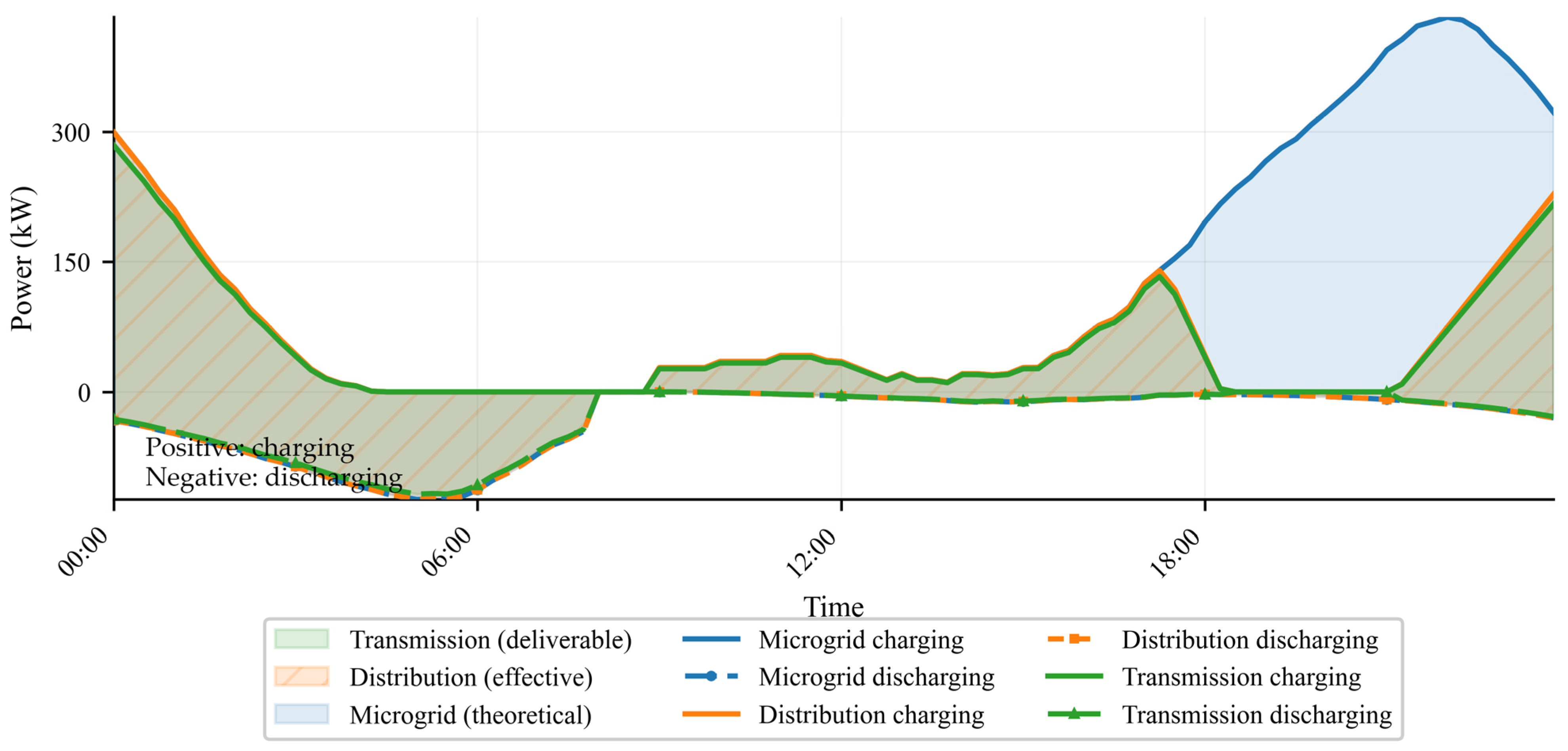
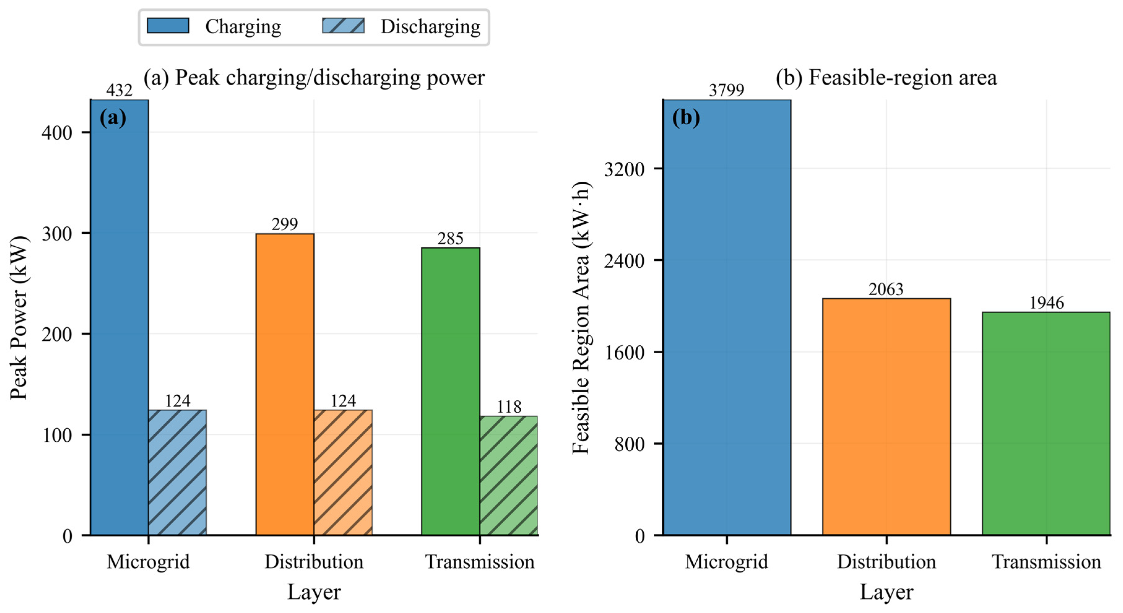
As shown in Figure 2, the three-layer envelopes exhibit a clear contraction pattern from microgrid theoretical capability to distribution-feasible capability and then to transmission deliverable capability. Quantitatively, the microgrid-layer envelope reaches 432 kW on the charging side, 124 kW on the discharging side, and 3799 kWh in feasible-region area. Under distribution constraints, the envelope is clipped to 299 kW, 124 kW, and 2063 kWh, while transmission-side packaging further yields 285 kW, 118 kW, and 1946 kWh. These results preserve the same layered interpretation as before, but under the revised formal baseline, they indicate a more pronounced contraction from station-side theoretical potential to upper-layer deliverable capability.
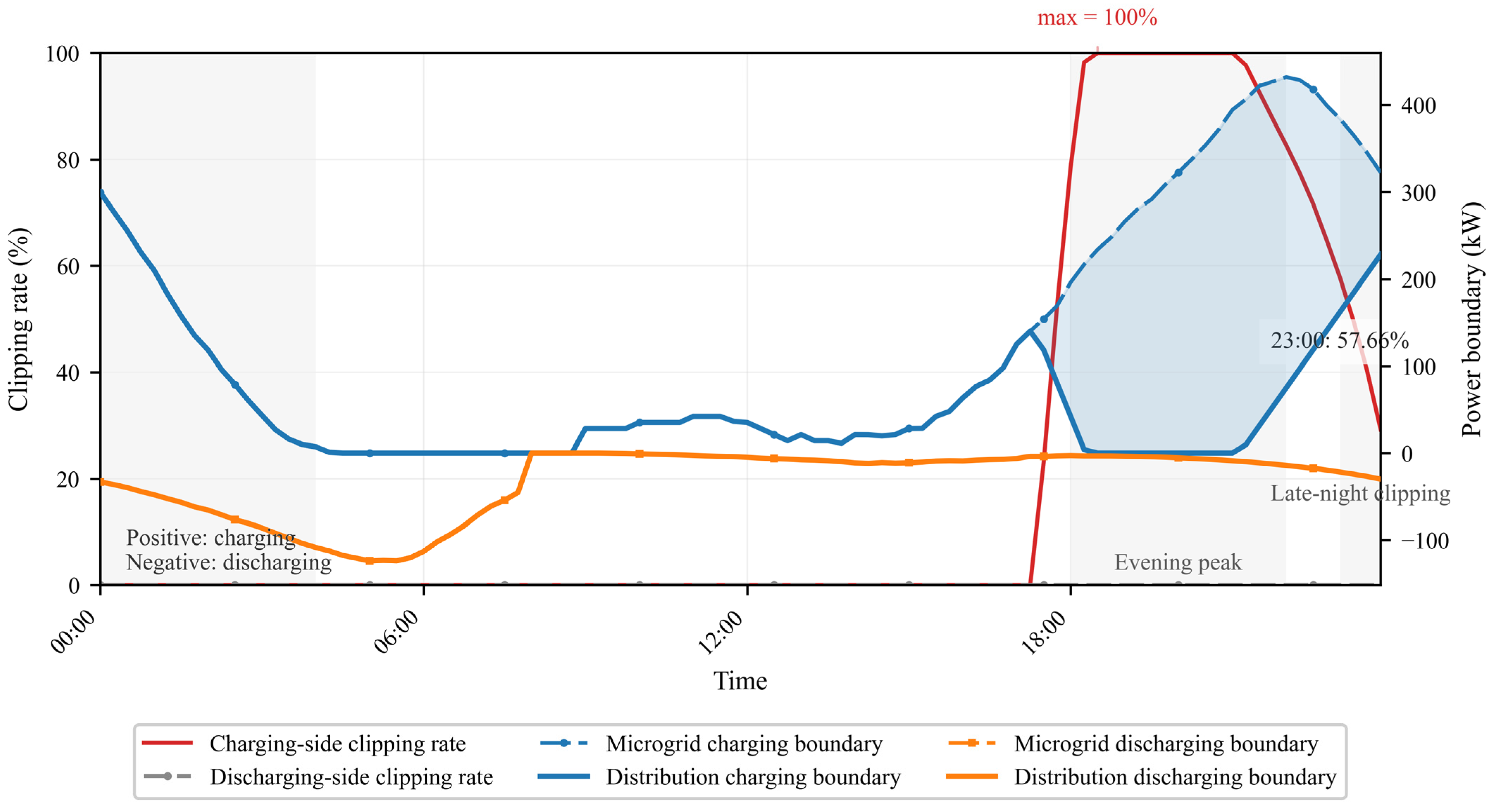
Figure 3 shows that clipping is dominated by the charging side during constrained periods. The mean charging-side clipping rate is 26.97%, and the maximum clipping rate reaches 100.00% at 18:30. At 23:00, the charging-side clipping rate remains significant at 57.66%. By contrast, the discharging-side clipping rate at both 18:30 and 23:00 is 0.00%, indicating that, under the present parameter setting, the main bottleneck is concentrated on charging-side deliverability during the evening-to-late-night interval.
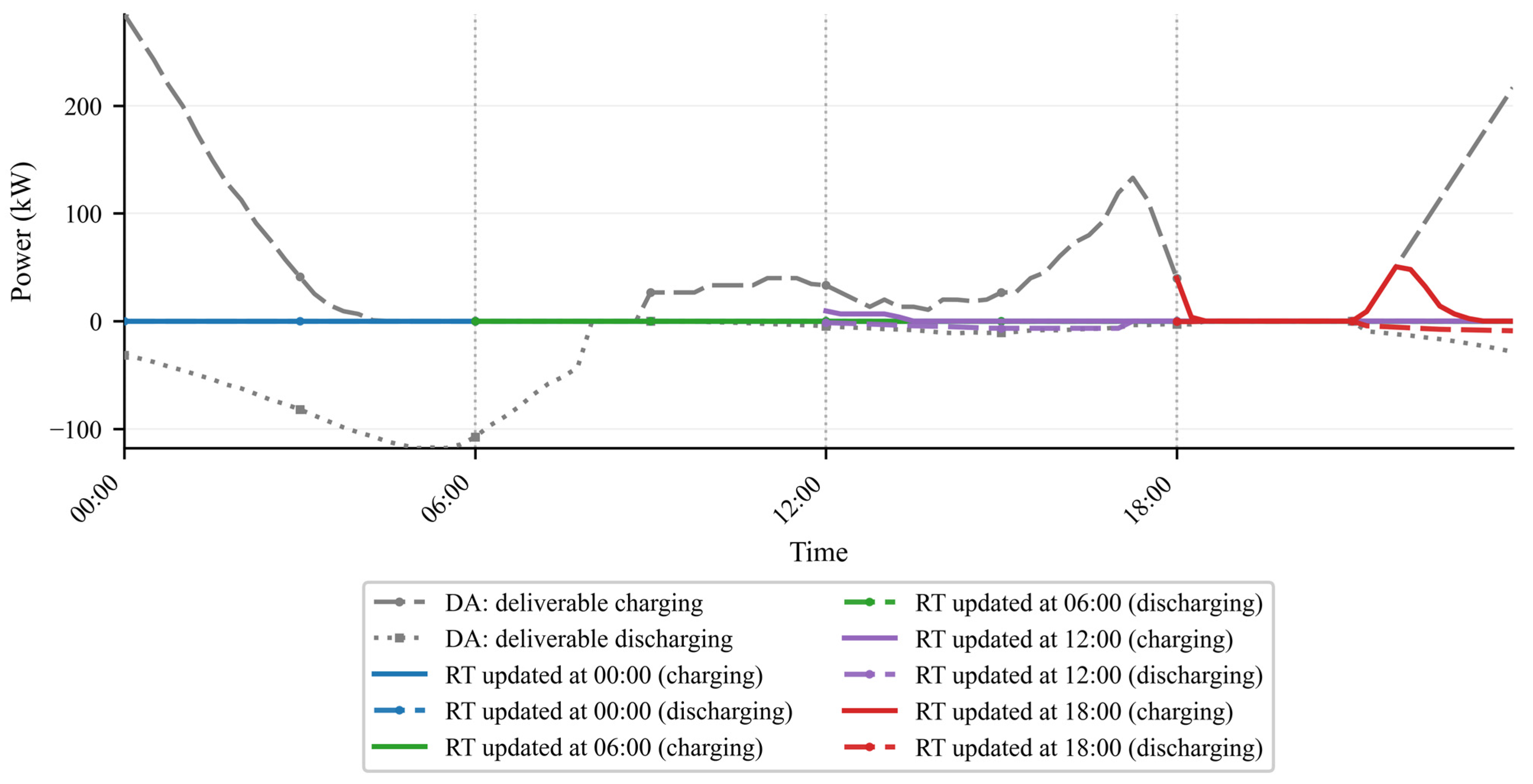
Figure 4 compares the transmission-layer deliverable boundaries in the day-ahead (DA) and real-time (RT) stages. The overall trends are consistent, but the RT boundary becomes more conservative at selected periods because the connected-EV set, SOC states, remaining dwell times, and network margins are updated online. These results suggest that day-ahead assessment provides a baseline range of adjustable capability, while real-time rolling mechanisms calibrate the boundary according to observed conditions. Figure 4 further illustrates the real-time deliverable envelopes updated at four representative observation instants (00:00, 06:00, 12:00, and 18:00); for each observation instant, only the remaining horizon is displayed so that the rolling-update effect can be interpreted consistently. The differences among the curves reflect the evolution of vehicle availability and security margins rather than a fixed deterministic shift.
The peak-and-area comparison in Figure 5 confirms that distribution-network constraints and transmission packaging affect both instantaneous and cumulative flexibility. Relative to the microgrid baseline of 432 kW, 124 kW, and 3799 kWh, the distribution layer exhibits reductions of 30.79% in peak charging capability, 0.00% in peak discharging capability, and 45.70% in envelope area. The transmission layer shows a larger overall contraction, with reductions of 34.03% in peak charging capability, 4.84% in peak discharging capability, and 48.78% in envelope area. This indicates that relying only on station-side theoretical flexibility would materially overestimate system-level deliverable capability.
A direct advantage of the hierarchical framework is that a vehicle-level high-dimensional problem is converted into a lower-dimensional computation of time-series boundaries plus constraint clipping. Because the workflow uses boundary sequences, scenario-wise aggregation, and linear clipping, the computation is markedly lighter than centralized joint vehicle-network optimization. The microgrid layer undertakes the main scenario generation and aggregation, the distribution layer performs linear feasibility clipping, and the transmission layer carries out lightweight conservative packaging. All simulations were implemented in Python 3.9.13 in an Anaconda environment on a Windows-based ASUS ROG laptop (2023 edition), equipped with a 13th Gen Intel Core i7-13650HX CPU and 32 GB RAM. The main numerical environment used NumPy 2.0.2, pandas 2.3.3, SciPy 1.13.1, and Matplotlib 3.9.4. For the T = 96 main case, the end-to-end wall-clock runtime, including scenario generation, aggregation, clipping, packaging, real-time conditioning, plotting, and consistency checking, was 21.50 s; the AC power-flow validation was performed using pandapower 2.14. Accordingly, the quoted computational complexity should be interpreted under this implementation logic—namely, scenario-wise boundary construction and parameter extraction—rather than as the cost of exact enumeration of a full high-dimensional Minkowski sum.
In summary, the proposed three-layer hierarchical assessment exhibits the computational characteristics of “microgrid-layer dominated computation, distribution-layer linear clipping, and transmission-layer lightweight packaging”. As constraints propagate upward, both peak power and feasible-region area shrink, and real-time rolling updates provide online correction of boundaries. This offers a more consistent “deliverable” capability characterization for subsequent dispatch and market-oriented applications.

4.2. Additional Validation of the Convex Relaxation Assumption

To quantify the error introduced by relaxing the mutual exclusivity between charging and discharging, we further conducted a benchmark comparison between the current convex-relaxed model and a mixed-integer linear programming (MILP) model with explicit charging/discharging exclusivity constraints. Since the full three-layer case involves 200 EVs, four charging stations, T = 96 time intervals, and scenario-wise aggregation, directly replacing the entire main workflow with a mixed-integer formulation would lead to a substantial computational burden. Therefore, this benchmark was carried out as a reduced station-level validation test on CS1 (day 1, nEV = 16) while preserving the same time resolution (T = 96) and confidence level (α = 0.90).
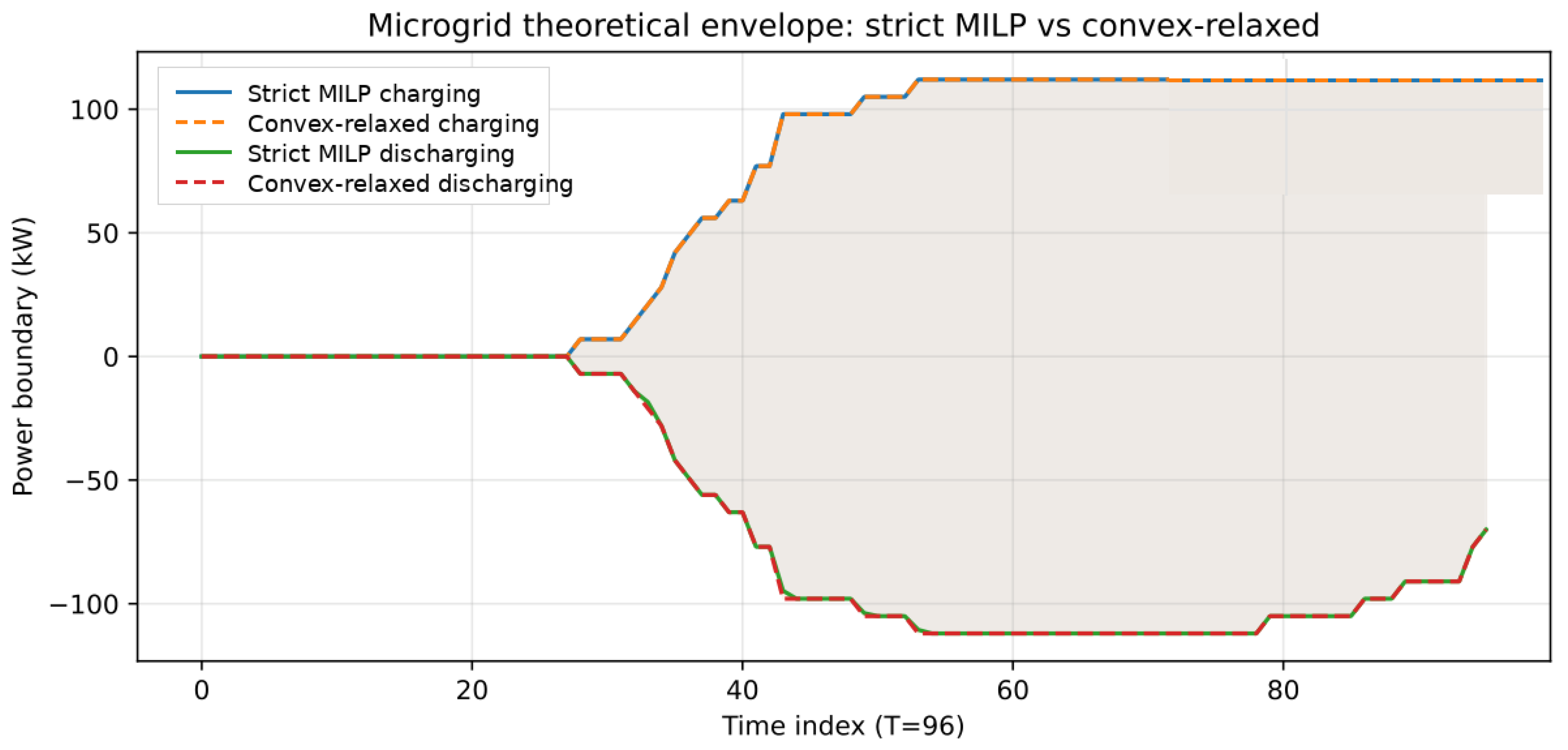
In the benchmark, the resulting theoretical envelope areas were 3062.50 kWh and 3060.36 kWh for the convex-relaxed and MILP formulations, respectively, yielding an absolute percentage deviation (APD) of only 0.0698%. In addition, the peak charging boundary remained unchanged at 112.0 kW, and the peak discharging boundary also remained unchanged at 112.0 kW for both formulations. These results indicate that, in the present benchmark, the convex relaxation does not cause severe capability overestimation in either the peak-power boundary or the envelope-area metric.
As shown in Figure 6, the two envelopes are nearly indistinguishable at the plotting scale, which is consistent with the very small APD reported in Table 2. From the computational perspective, the convex-relaxed benchmark required 12.07 s, whereas the MILP benchmark required 45.16 s. Therefore, the convex-relaxed formulation is retained in the main assessment workflow as a computationally efficient boundary representation, with its approximation error now explicitly quantified.
The near overlap of the two envelopes also indicates that, under the adopted inner-envelope benchmark, the charging/discharging mutual-exclusivity constraint rarely changes the envelope-defining points. In practical terms, most boundary-supporting vehicle–time realizations in the tested setting are either idle or single-directional, so the convex relaxation has limited opportunity to generate additional area.
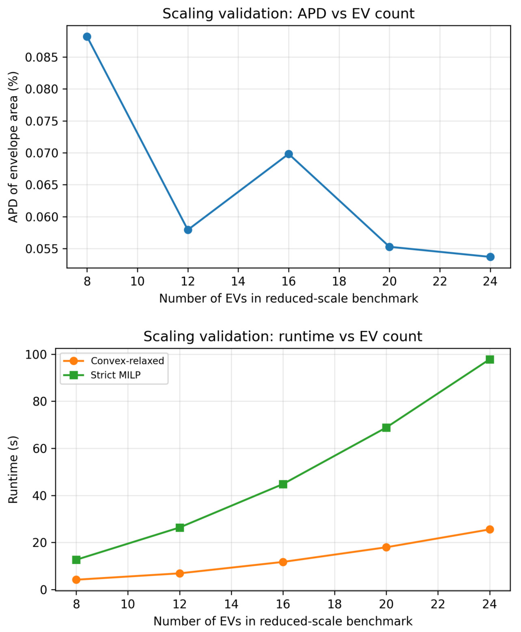
To further examine whether this conclusion remains valid as the benchmark size increases, we carried out a scaling validation with nEV = 8, 12, 16, 20, and 24 under the same station-level benchmark setting while keeping T = 96, α = 0.90, and the same scenario-generation and envelope-construction logic. Across the tested sizes, the APD remains very small, with a mean value of 0.0650% and a maximum value of 0.0882%. Moreover, the peak charging and discharging boundaries remain unchanged for all tested sizes, indicating that the relaxation-induced error is not only small in the representative 16-EV benchmark but also stable across the tested reduced-scale range.
As shown in Figure 7 and Table 3, the APD does not increase with benchmark size and stays below 0.1% throughout the tested range, whereas the MILP runtime grows much faster than that of the convex-relaxed formulation. On average, the MILP runtime is 3.67 times the convex-relaxed runtime in the tested reduced-scale cases. Therefore, the mixed-integer formulation is used here as a representative fidelity check for the convex-relaxed boundary model, while the full main-case workflow continues to adopt the convex-relaxed formulation to maintain tractable large-scale hierarchical assessment.

4.3. Sensitivity to Confidence Level

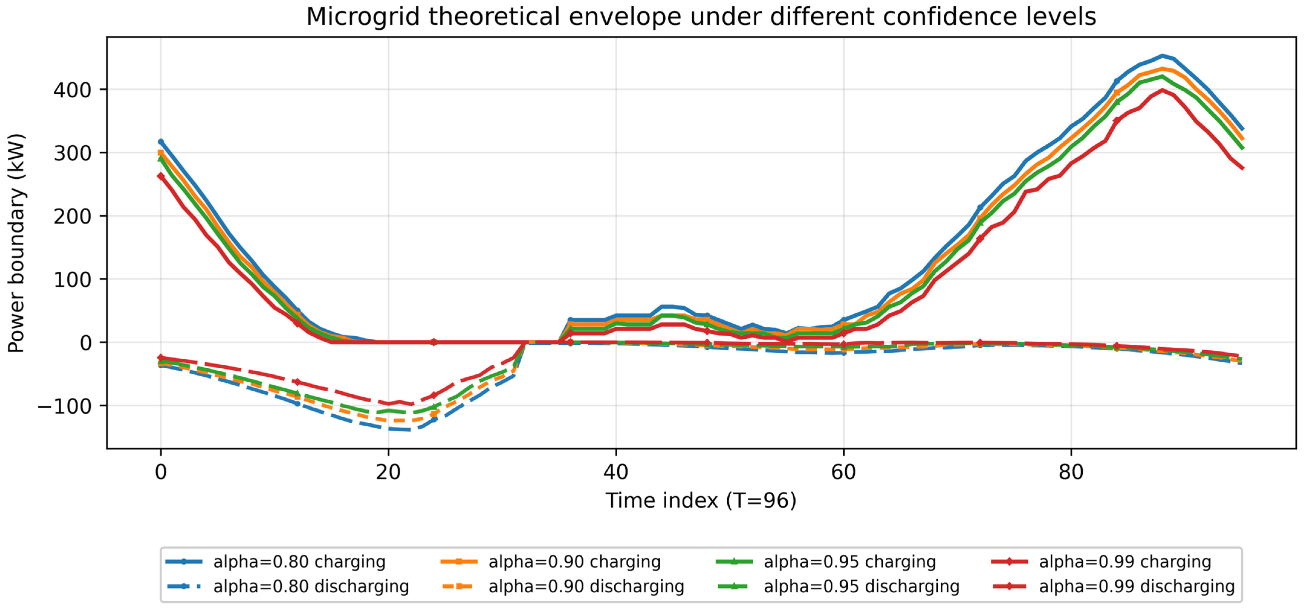
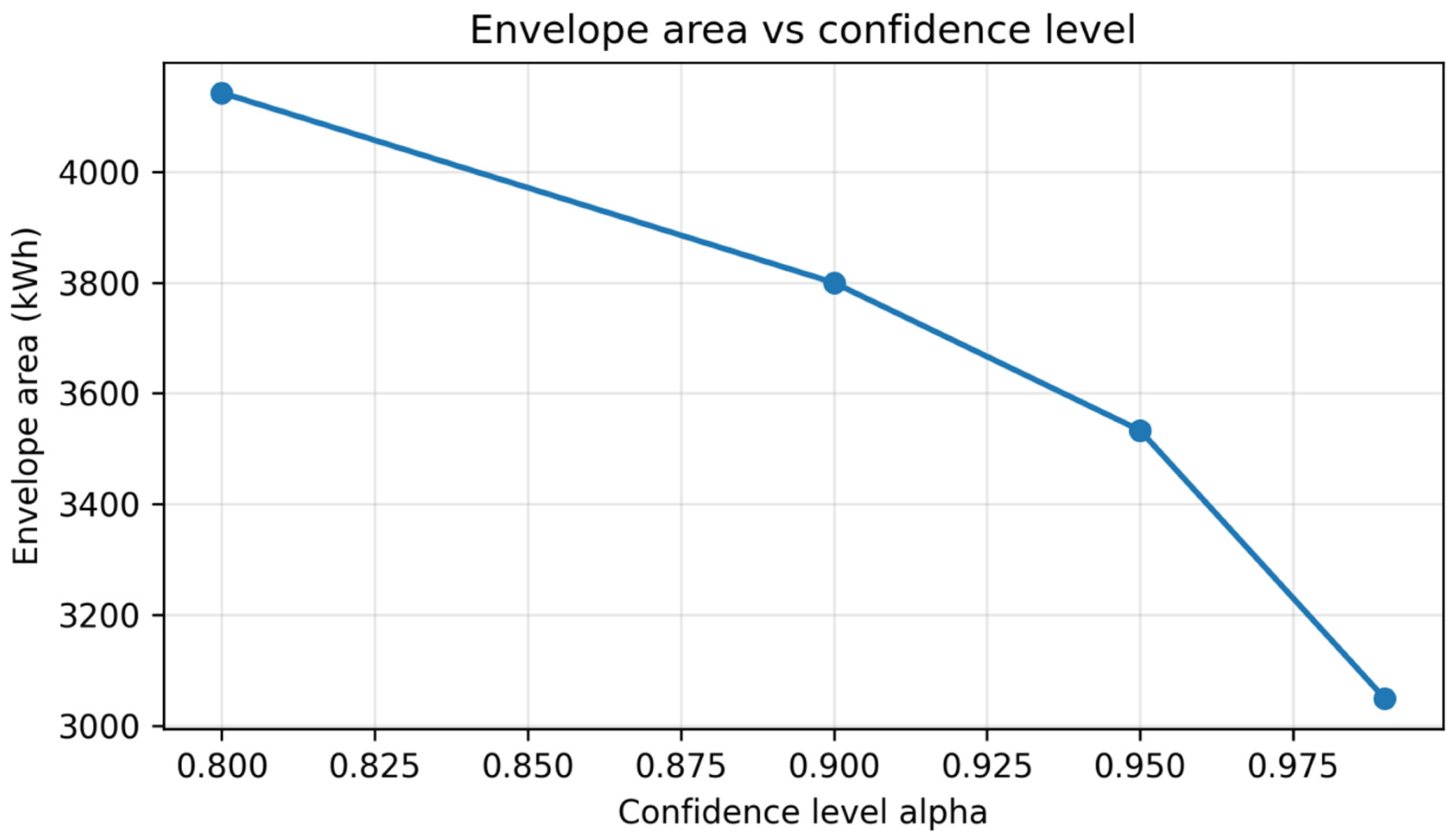
To examine the sensitivity of the inner-envelope construction to the confidence parameter, we further evaluate the microgrid-layer theoretical envelope for α = 0.80, 0.90, 0.95, and 0.99 under the same Gaussian-copula scenario set and aggregation pipeline. The results are summarized in Table 4 and Figure 8 and Figure 9. The results show a monotonic contraction of the inner envelope as α increases. Specifically, the peak charging boundary decreases from 452.8 kW at α = 0.80 to 398.3 kW at α = 0.99, the peak discharging boundary decreases from 138.2 kW to 98.1 kW, and the envelope area decreases from 4142.2 kWh to 3048.8 kWh. At the baseline confidence level α = 0.90, the corresponding values are 432.2 kW, 124.2 kW, and 3799.5 kWh, respectively. These trends indicate that a higher confidence requirement yields a more conservative inner approximation, which is consistent with the deliverability-oriented interpretation of the proposed boundary-assessment framework.

4.4. AC Cross-Validation of LinDistFlow at Severe-Clipping Cross Sections

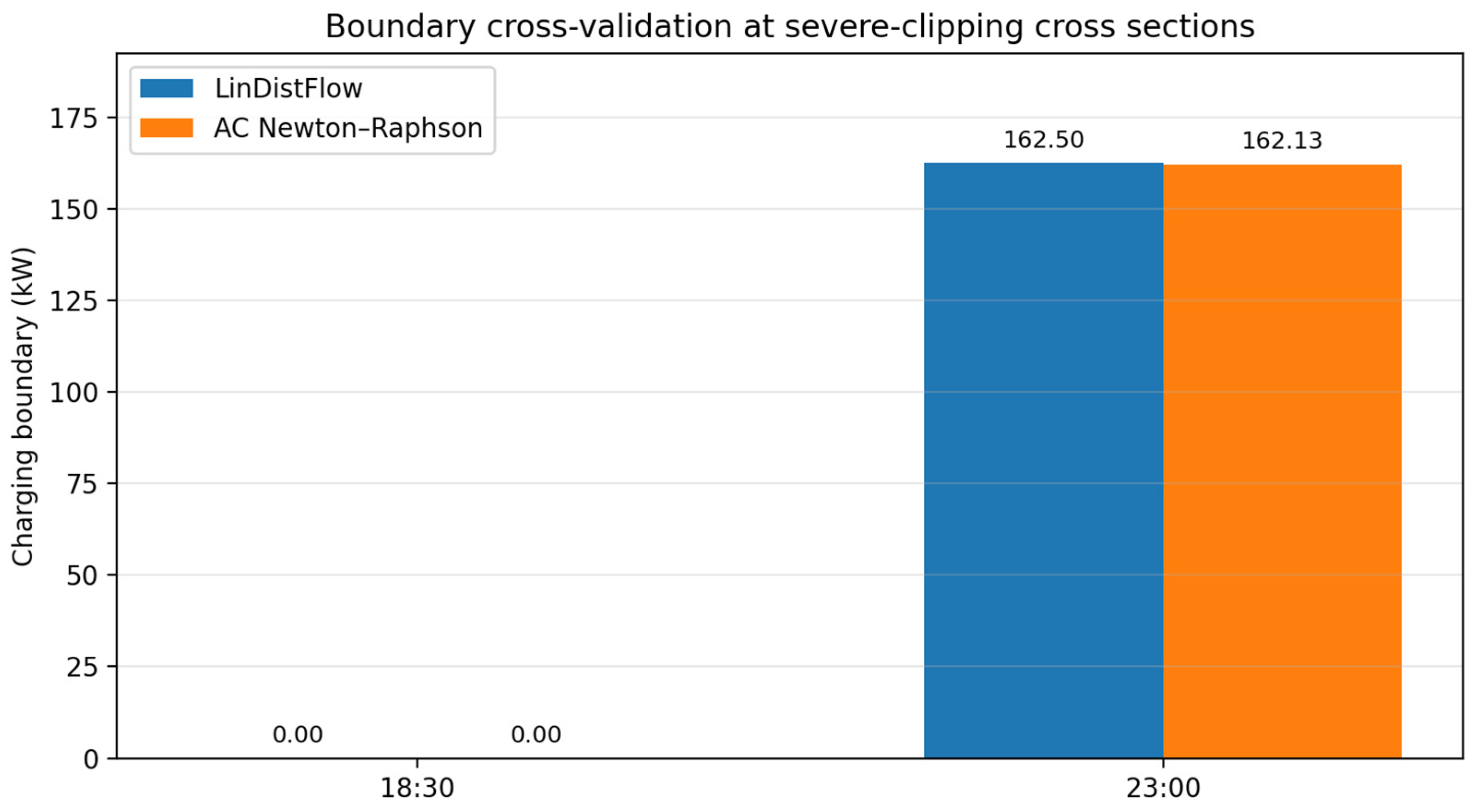
Because the maximum charging-side clipping occurs at 18:30 and remains significant at 23:00, we further cross-validate the LinDistFlow-based charging boundaries at these two representative cross sections using a Newton–Raphson AC power-flow model implemented in pandapower. To ensure consistency with the main case, the AC cross-check adopts the same 33-bus feeder, the same Gaussian-copula scenario set, the same uniform scaling of station-level charging injections, and the same inner-envelope quantile definition used in the LinDistFlow-based assessment. It should also be noted that the 18:30 coincidence of the LinDistFlow and AC boundaries is primarily driven by exhaustion of substation headroom, which is represented identically in both formulations, rather than by the voltage or thermal constraints that LinDistFlow linearizes. Accordingly, the 23:00 cross section, where the minimum AC voltage is closer to the admissible lower bound, provides the more direct fidelity test of the LinDistFlow approximation. The resulting boundary comparison is shown in Figure 10.
Table 5 summarizes the boundary comparison. At 18:30, both the LinDistFlow model and the AC model yield a zero charging boundary under the adopted inner-envelope definition, which confirms the 100% clipping conclusion at the evening peak rather than attributing it to a linearization artifact. At 23:00, the LinDistFlow and AC charging boundaries are 162.50 kW and 162.13 kW, respectively, corresponding to a relative deviation of only 0.23%. The minimum AC voltages at 18:30 and 23:00 are 0.9651 p.u. and 0.9576 p.u., respectively. These results indicate that the severe charging-side clipping reported in the main case is physically credible under the adopted conservative inner-envelope representation, while the 23:00 boundary is also closely matched between LinDistFlow and AC.

4.5. Full-Day Multi-Period AC-Based Joint P–Q Feasible-Boundary Projection

To strengthen the network-level interpretation beyond active-power-only clipping, this revision upgrades the joint P–Q analysis from a representative single-time illustration to a full-day, multi-period AC-based feasible-boundary projection over all 96 time intervals. The aim is to characterize how aggregate active–reactive flexibility evolves throughout the day under the same time-varying load/PV background and distribution-network security limits.
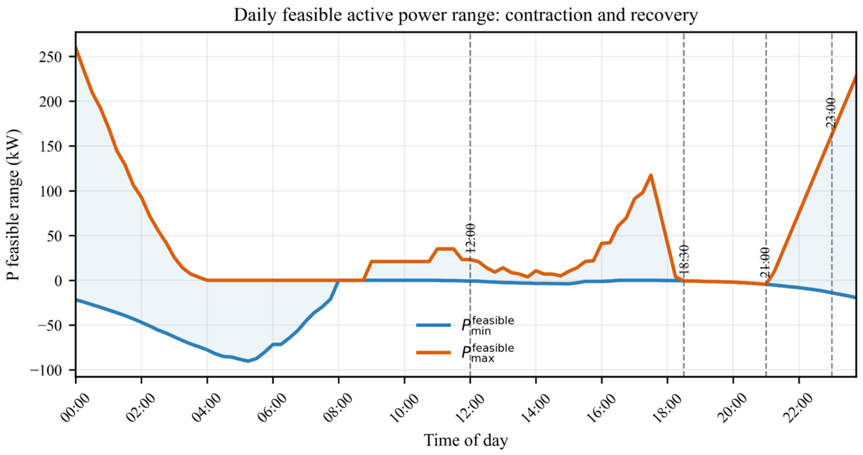
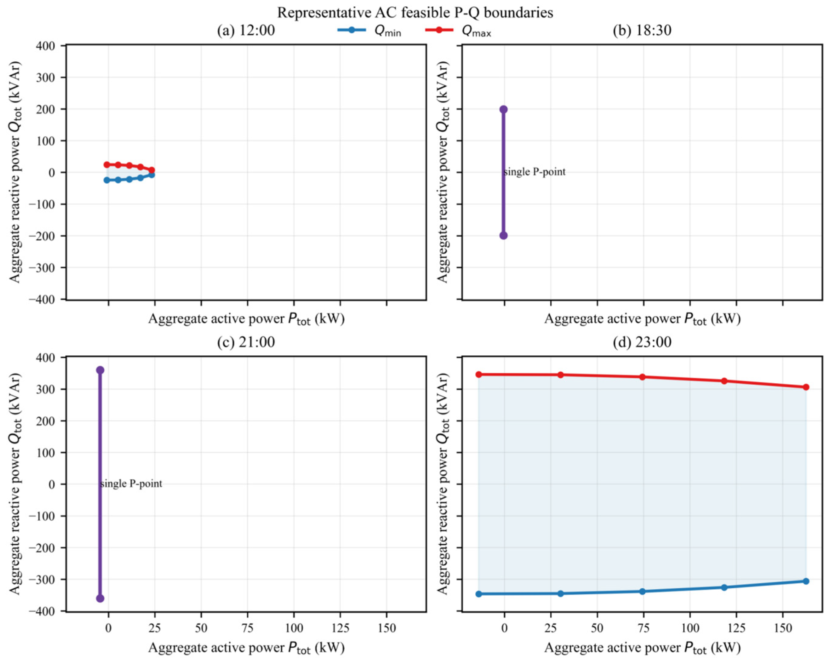
At each time index t, the four charging stations are modeled as independently adjustable injections (Pj,t, Qj,t) rather than being constrained by a fixed proportional-allocation rule. For each aggregate active-power grid point Ptot,t, this study determines the corresponding feasible reactive envelope by identifying the upper and lower bounds Qtot,tmax and Qtot,tmin under, (i) station active-power bounds, (ii) station apparent-power limits Pj,t2 + Qj,t2 ≤ (Sj,tmax)2, and (iii) AC power-flow feasibility with nodal-voltage constraints, branch thermal limits, and feeder-head active-power headroom. This yields a time-resolved AC-feasible projected boundary approximation in the (Ptot, Qtot) plane for each time period. Representative active–reactive feasible ranges are summarized in Table 6.
Figure 11 shows the day-long evolution of the feasible aggregate active-power range, revealing a clear pattern of contraction during the evening peak and recovery afterward. Figure 12 further compares representative projected boundaries at 12:00, 18:30, 21:00, and 23:00. The 12:00 case represents a daytime non-degenerate feasible region, whereas 23:00 serves as a post-peak recovery reference with a substantially reopened boundary. In contrast, the feasible boundaries at 18:30 and 21:00 contract so strongly that the projected set degenerates to a single-P cross section. This degenerate presentation should be interpreted as a physical contraction of the AC-feasible set under network-security limits at those periods, rather than as a numerical artifact or a plotting error. At these two times, the active-power degree of freedom is effectively pinned by the binding network constraints, while a residual reactive interval remains feasible at the fixed active-power point; hence the vertical single-P slices in Figure 12 are expected outcomes of the AC-feasible projection.
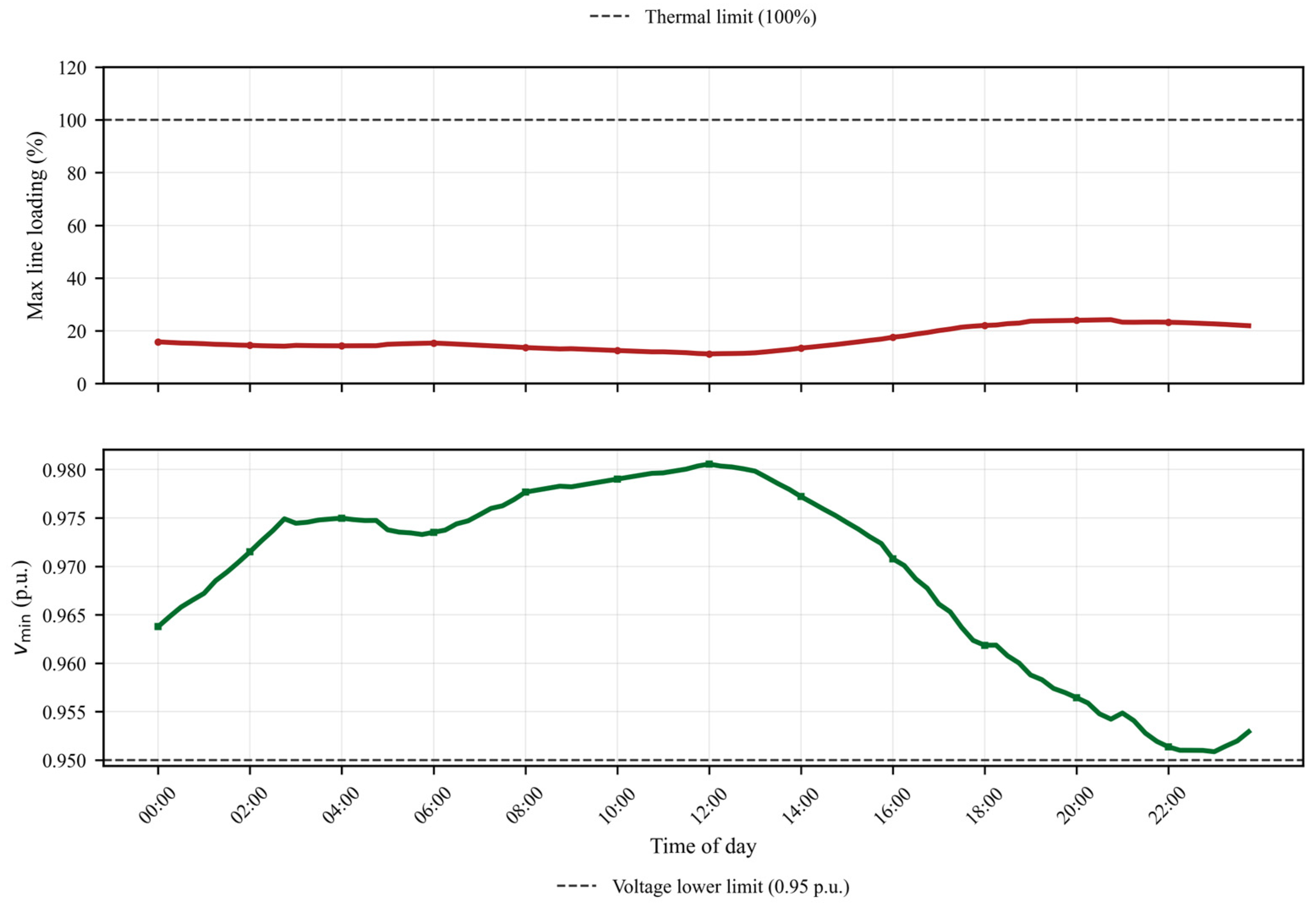
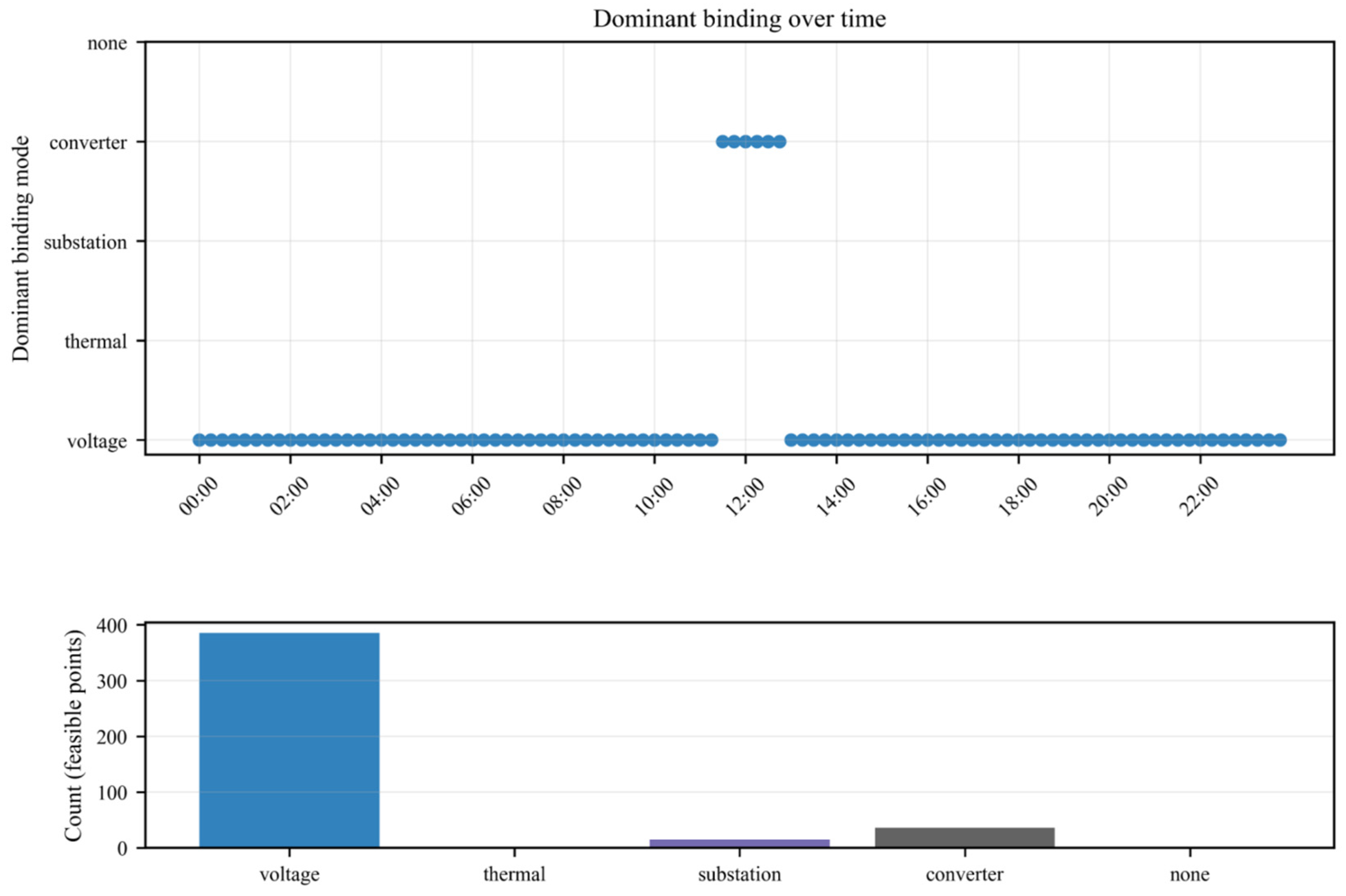
Figure 13 explains the mechanism behind this contraction. Across the day, line-loading levels remain well below the thermal limit, while the minimum-voltage trajectory approaches the lower admissible bound more closely during the tight evening intervals. Figure 14 further shows that the dominant binding factor is non-thermal and shifts with operating conditions: converter limits dominate many lightly stressed periods, the degenerate point at 18:30 is identified as substation-headroom-limited, and the degenerate point at 21:00 is voltage-limited. Here, the time-axis classification identifies the dominant binding mode at the time-step level, while the count statistics summarize dominant labels over all feasible boundary points. Therefore, the evening boundary collapse should be interpreted as a network-side AC-feasibility contraction in which substation headroom and voltage constraints become active at different stressed periods, rather than as a thermal-overload phenomenon.
Overall, the full-day AC-based projection provides a time-resolved joint P–Q feasibility picture that is consistent with the main clipping analysis and suitable for system-level operational interpretation. The earlier proportional-allocation slice is retained only as a historical simplified comparison and is no longer used as the primary result path.

5. Conclusions

This paper proposes a hierarchical adjustable-potential assessment framework for aggregated EV resources in transmission–distribution–microgrid coordination. Rather than seeking a dispatch trajectory, the framework provides a consistent pathway from station-side theoretical envelopes to distribution-feasible effective potential and finally to transmission-readable deliverable boundaries for both day-ahead and real-time use.
The revised main-case results further support the same core conclusion: layered network constraints systematically compress EV flexibility from theoretical station-side potential to system-level deliverable potential. In the present case, the microgrid-layer envelope reaches 432 kW on the charging side, 124 kW on the discharging side, and 3799 kWh in feasible-region area; the distribution layer reduces these values to 299 kW, 124 kW, and 2063 kWh; and the transmission layer further reduces them to 285 kW, 118 kW, and 1946 kWh. Relative to the microgrid baseline, this corresponds to reductions of 30.79% in peak charging capability, 0.00% in peak discharging capability, and 45.70% in feasible-region area at the distribution layer, and 34.03%, 4.84%, and 48.78%, respectively, at the transmission layer. Charging-side clipping remains the dominant bottleneck, with a mean clipping rate of 26.97%, a maximum of 100.00% at 18:30, and 57.66% at 23:00, whereas discharging-side clipping at these two representative times remains 0.00%. Therefore, station-side theoretical potential should not be directly interpreted as dispatchable upper-layer capability without distribution-layer clipping and transmission-oriented packaging.
From an application perspective, the transmission-layer deliverable boundary can support capacity declaration, ancillary-service qualification, and demand-response validation without overstating downstream capability. The proposed bottleneck truncation effect provides a useful diagnostic index for DSOs to identify periods and locations where downstream constraints most strongly truncate upstream-reportable flexibility. In addition, because only aggregated boundary parameters are reported upward, the framework supports privacy-preserving coordination at the information-interface level rather than through exchange of individual EV trajectories or raw user-level charging records. The core T = 96 hierarchical workflow was completed in 21.50 s on a standard laptop platform, indicating that the proposed assessment framework remains computationally practical for repeated case-based analysis and rolling boundary updates. The very small APD therefore reflects engineering acceptability of the relaxation in the tested benchmark setting rather than an absence of physical mutual-exclusivity logic in the strict MILP formulation.
Moreover, the scenario-generation module was revised using a Gaussian-copula-based correlated sampling scheme so that the main dependence patterns among arrival time, departure time, and initial SOC can be better preserved than under independent resampling. The copula dependence is calibrated from the empirical behavior sample underlying the case study, thereby keeping the joint behavior model data-grounded at the scenario-generation stage. A confidence-level sensitivity analysis over α = 0.80, 0.90, 0.95, and 0.99 further showed that the microgrid-layer inner envelope shrinks monotonically as the confidence requirement increases, which supports the deliverability-oriented interpretation of the proposed inner-approximation framework.
Finally, the reactive-power assessment was upgraded from representative cross-sectional slices to a full-day, 96-period AC-based P–Q feasible-boundary projection. The revised results show a daytime non-degenerate feasible region at 12:00, severe contraction to single-P cross-sections at 18:30 and 21:00, and substantial reopening at 23:00. Combined with the network-security metrics and dominant-binding analysis, this indicates that the observed evening collapse is driven by substation-headroom exhaustion at 18:30 and voltage limitation at 21:00 rather than by thermal overload. These results confirm that the legacy proportional-allocation slice was overly idealized for representing the actual active–reactive feasible boundary under stressed operating conditions.
Future work can refine the present full-day AC-based projected boundary approximation into a fully optimized multi-period AC-OPF reactive-flexibility formulation, adopt richer data-driven scenario generation or generative models, examine sensitivity with respect to the scenario number M and the boundary-resolution settings, benchmark larger-scale multi-feeder cases, and broaden the present AC validation to more comprehensive network-feasibility verification.

Author Contributions

Conceptualization, M.W.; methodology, M.W.; software, Y.P.; validation, W.R.; formal analysis, M.W.; investigation, H.G.; resources, K.D.; data curation, Y.P.; writing—original draft preparation, M.W.; writing—review and editing, X.Y.; visualization, Y.P.; supervision, X.Y.; project administration, H.G.; funding acquisition, H.G. All authors have read and agreed to the published version of the manuscript.

Funding

This research was funded by State Grid Jiangsu Electric Power Co., Ltd., grant number J2024152. The project title is “Research on Vehicle-to-Grid Interaction Flexibility Enhancement Technology for Transmission-Distribution-Microgrid Coordination”.

Data Availability Statement

Data are available from the corresponding author upon reasonable request. The data are not publicly available due to privacy or ethical restrictions.

Conflicts of Interest

Authors Mingshen Wang, Yi Pan, Xiaodong Yuan, and Kemin Dai were employed by the company Electric Power Research Institute, Jiangsu Power Grid Company Ltd. Authors Wenjun Ruan and Haiqing Gan were employed by the company Jiangsu Power Grid Company Ltd. The authors declare that this study received funding from State Grid Jiangsu Electric Power Co., Ltd. The funder was not involved in the study design, collection, analysis, interpretation of data, the writing of this article, or the decision to submit it for publication.

References

  1. Callaway, D.S.; Hiskens, I.A. Achieving Controllability of Electric Loads. Proc. IEEE 2011, 99, 184–199. [Google Scholar] [CrossRef]
  2. Huang, A.Q.; Crow, M.L.; Heydt, G.T.; Zheng, J.P.; Dale, S.J. The Future Renewable Electric Energy Delivery and Management (FREEDM) System: The Energy Internet. Proc. IEEE 2011, 99, 133–148. [Google Scholar] [CrossRef]
  3. Sovacool, B.K.; Kester, J.; Noel, L.; de Rubens, G.Z. Actors, Business Models, and Innovation Activity Systems for Vehicle-to-Grid (V2G) Technology: A Comprehensive Review. Renew. Sustain. Energy Rev. 2020, 131, 109963. [Google Scholar] [CrossRef]
  4. Kempton, W.; Tomic, J. Vehicle-to-Grid Power Fundamentals: Calculating Capacity and Net Revenue. J. Power Sources 2005, 144, 268–279. [Google Scholar] [CrossRef]
  5. Kempton, W.; Tomic, J. Vehicle-to-Grid Power Implementation: From Stabilizing the Grid to Supporting Large-Scale Renewable Energy. J. Power Sources 2005, 144, 280–294. [Google Scholar] [CrossRef]
  6. Xu, Z.; Su, W.; Hu, Z.; Song, Y.; Zhang, H. A Hierarchical Framework for Coordinated Charging of Plug-In Electric Vehicles in China. IEEE Trans. Smart Grid 2016, 7, 428–438. [Google Scholar] [CrossRef]
  7. Gerard, H.; Rivero Puente, E.I.; Six, D. Coordination between Transmission and Distribution System Operators in the Electricity Sector: A Conceptual Framework. Util. Policy 2018, 50, 40–48. [Google Scholar] [CrossRef]
  8. Wang, Y.; Infield, D. Markov Chain Monte Carlo Simulation of Electric Vehicle Use for Network Integration Studies. Int. J. Electr. Power Energy Syst. 2018, 99, 85–94. [Google Scholar] [CrossRef]
  9. Sortomme, E.; El-Sharkawi, M.A. Optimal Charging Strategies for Unidirectional Vehicle-to-Grid. IEEE Trans. Smart Grid 2011, 2, 131–138. [Google Scholar] [CrossRef]
  10. Gan, L.; Topcu, U.; Low, S.H. Optimal Decentralized Protocol for Electric Vehicle Charging. IEEE Trans. Power Syst. 2013, 28, 940–951. [Google Scholar] [CrossRef]
  11. Jian, L.; Zheng, Y.; Xiao, X.; Chan, C.C. Optimal Scheduling for Vehicle-to-Grid Operation with Stochastic Connection of Plug-In Electric Vehicles to Smart Grid. Appl. Energy 2015, 146, 150–161. [Google Scholar] [CrossRef]
  12. Müller, F.L.; Szabó, J.; Sundström, O.; Lygeros, J. Aggregation and Disaggregation of Energetic Flexibility from Distributed Energy Resources. IEEE Trans. Smart Grid 2019, 10, 1205–1214. [Google Scholar] [CrossRef]
  13. Nazir, M.S.; Hiskens, I.A.; Bernstein, A.; Dall’Anese, E. Inner Approximation of Minkowski Sums: A Union-Based Approach and Applications to Aggregated Energy Resources. In Proceedings of the 2018 IEEE Conference on Decision and Control (CDC); NREL Conference Paper NREL/CP-5D00-73423; IEEE: New York, NY, USA, 2019. [Google Scholar]
  14. Bolognani, S.; Zampieri, S. On the Existence and Linear Approximation of the Power Flow Solution in Power Distribution Networks. IEEE Trans. Power Syst. 2016, 31, 163–172. [Google Scholar] [CrossRef]
  15. Zhang, L.; Ji, Y.; Li, X.; Huang, Z.; Cui, D.; Chen, H.; Gong, J.; Breer, F.; Junker, M.; Sauer, D.U. Multi-objective Charging Scheduling for Electric Vehicles at Charging Stations with Renewable Energy Generation. Green Energy Intell. Transp. 2025, 4, 100283. [Google Scholar] [CrossRef]
  16. Ray, S.; Kasturi, K.; Nayak, M.R. Multi-objective Electric Vehicle Charge Scheduling for Photovoltaic and Battery Energy Storage Based Electric Vehicle Charging Stations in Distribution Network. Green Energy Intell. Transp. 2025, 4, 100296. [Google Scholar] [CrossRef]
  17. Yaghoubi, E.; Yaghoubi, E.; Khamees, A.; Razmi, D.; Lu, T. A Systematic Review and Meta-analysis of Machine Learning, Deep Learning, and Ensemble Learning Approaches in Predicting EV Charging Behavior. Eng. Appl. Artif. Intell. 2024, 135, 108789. [Google Scholar] [CrossRef]
  18. Maghami, M.R.; Thang, K.F.; Mutambara, A.G.O.; Firoozi, A.A.; Yaghoubi, E.; Zareian Jahromi, M.; Yaghoubi, E. Optimized Planning of Electric Vehicle Charging Infrastructure for Grid Performance Improvement. Discov. Sustain. 2025, 6, 706. [Google Scholar] [CrossRef]
  19. Baran, M.E.; Wu, F.F. Network Reconfiguration in Distribution Systems for Loss Reduction and Load Balancing. IEEE Trans. Power Deliv. 1989, 4, 1401–1414. [Google Scholar] [CrossRef]
  20. Baran, M.E.; Wu, F.F. Optimal Sizing of Capacitors Placed on a Radial Distribution System. IEEE Trans. Power Deliv. 1989, 4, 735–743. [Google Scholar] [CrossRef]
  21. Farivar, M.; Low, S.H. Branch Flow Model: Relaxations and Convexification—Part I. IEEE Trans. Power Syst. 2013, 28, 2554–2564. [Google Scholar] [CrossRef]
  22. Low, S.H. Convex Relaxation of Optimal Power Flow—Part I: Formulations and Equivalence. IEEE Trans. Control Netw. Syst. 2014, 1, 15–27. [Google Scholar] [CrossRef]
  23. Bertsimas, D.; Sim, M. The Price of Robustness. Oper. Res. 2004, 52, 35–53. [Google Scholar] [CrossRef]
  24. Boyd, S.; Vandenberghe, L. Convex Optimization; Cambridge University Press: Cambridge, UK, 2004; ISBN 978-0521833783. [Google Scholar]
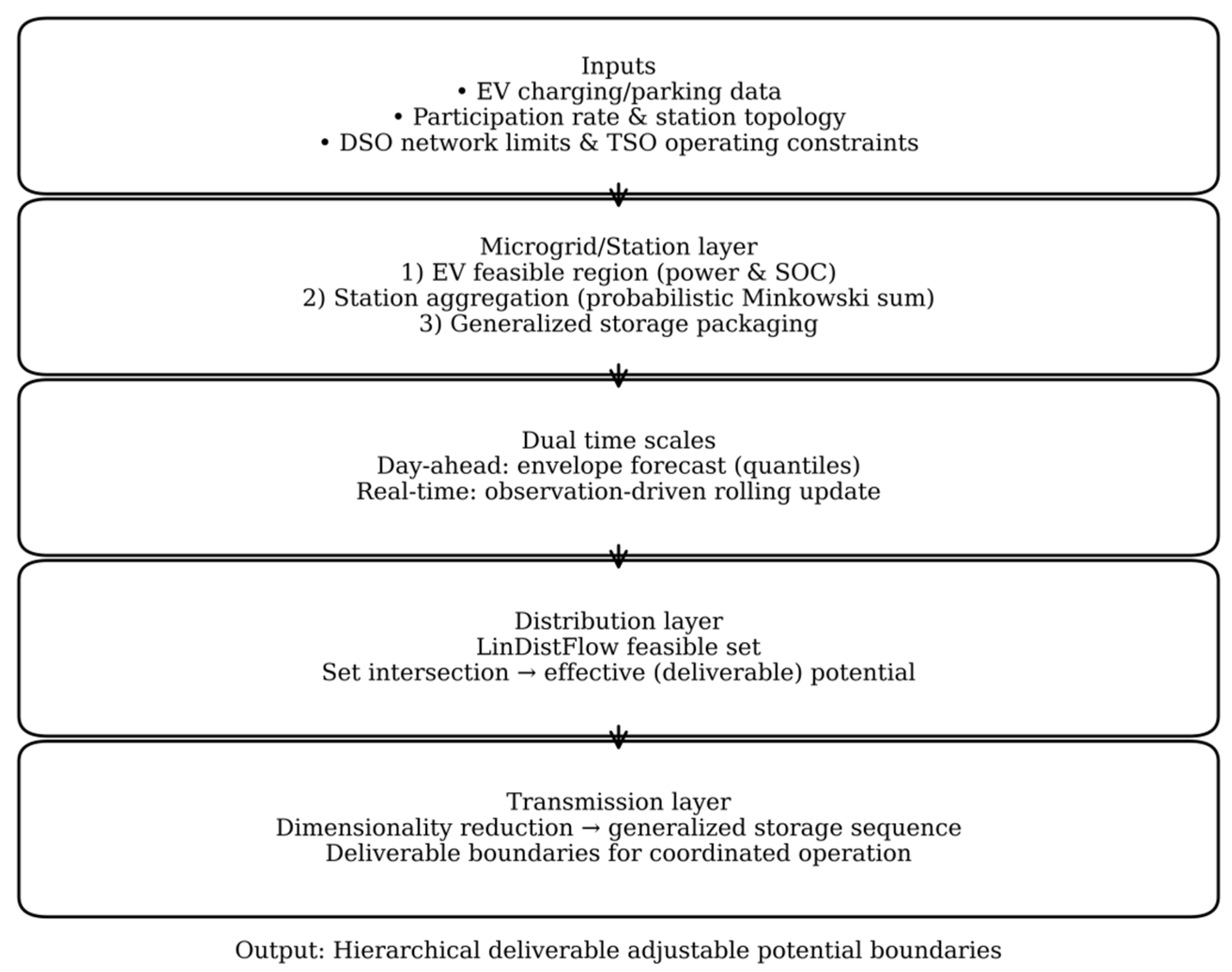
Figure 1. Overall hierarchical adjustable-potential assessment workflow. Note: the workflow links microgrid aggregation, distribution-layer clipping, and transmission-layer packaging.
Processes 14 01672 g001
Figure 2. Three-layer potential envelopes over the study horizon. Note: the layers are the microgrid theoretical envelope, distribution effective envelope, and transmission deliverable envelope; positive and negative power denote charging- and discharging-side boundaries, respectively.
Processes 14 01672 g002
Figure 3. Distribution-layer clipping rates over time. Note: charging- and discharging-side envelopes are shown; annotations mark the maximum clipping point at 18:30 and the late-night point at 23:00.
Processes 14 01672 g003
Figure 4. Day-ahead and real-time transmission-layer deliverable boundaries. Note: the figure compares day-ahead and real-time envelopes and shows real-time updates at 00:00, 06:00, 12:00, and 18:00 over the remaining horizon. Positive and negative power denote charging- and discharging-side capability, respectively.
Processes 14 01672 g004
Figure 5. Layer-wise comparison across layers: (a) peak charging/discharging power; (b) feasible-region area.
Processes 14 01672 g005
Figure 6. Station-level theoretical envelopes under convex-relaxed and MILP models. Note: the MILP benchmark enforces explicit charging/discharging mutual-exclusivity constraints.
Processes 14 01672 g006
Figure 7. Scaling validation of the convex-relaxation benchmark. Note: the upper panel reports theoretical-envelope APD versus EV number, and the lower panel compares convex-relaxed and strict MILP runtimes.
Processes 14 01672 g007
Figure 8. Microgrid-layer inner envelopes under different confidence levels. Note: the confidence levels are α = 0.80, 0.90, 0.95, and 0.99.
Processes 14 01672 g008
Figure 9. Microgrid-layer envelope area versus confidence level α.
Processes 14 01672 g009
Figure 10. LinDistFlow and AC-validated charging boundaries. Note: the representative severe-clipping cross sections are 18:30 and 23:00.
Processes 14 01672 g010
Figure 11. Daily feasible aggregate active-power range. Note: the boundary contracts during the evening peak and recovers afterward.
Processes 14 01672 g011
Figure 12. Representative AC-based P–Q feasible boundaries. Note: the representative times are 12:00, 18:30, 21:00, and 23:00.
Processes 14 01672 g012
Figure 13. Network security metrics in the AC-based P–Q projection. Note: the metrics are maximum line loading and minimum voltage.
Processes 14 01672 g013
Figure 14. Dominant-binding modes in the full-day AC-based P–Q projection. Note: time-step labels identify the dominant binding mode, and feasible-point counts summarize dominant labels over boundary points. In degenerate single-P cases, residual reactive intervals may remain feasible.
Processes 14 01672 g014
Table 1. Spearman rank-correlation comparison for CS1.
Variable PairEmpirical SampleCopula-Generated Sample (M = 500)Absolute Gap
Arrival time vs. departure time−0.1851−0.17320.0119
Arrival time vs. initial SOC (kWh)−0.6152−0.59730.0179
Departure time vs. initial SOC (kWh)0.22550.23410.0086
Note: The empirical sample is taken from the CS1 charger-pool dataset after removing rows with missing values in arrival time, departure time, and initial SOC. The copula-generated sample is obtained by regenerating a full M = 500 sample using the same random seed and the same main-pipeline Gaussian-copula fitting, sampling, and matching procedure as the case-study workflow, rather than from the preview file used only for diagnostic visualization.
Table 2. Convex-relaxed and MILP benchmark comparison.
ModelEnvelope Area (kWh)Peak Charging Boundary (kW)Peak Discharging Boundary (kW)Runtime (s)
Convex-relaxed3062.50112.0112.012.07
MILP with mutual exclusivity3060.36112.0112.045.16
APD0.0698%---
Note: The MILP benchmark includes explicit charging/discharging mutual-exclusivity constraints.
Table 3. Scaling validation of convex-relaxed and strict MILP formulations.
nEVAPD (%)Peak Ch. Diff. (kW)Peak Dis. Diff. (kW)MILP/Convex Runtime
80.08820.00.03.04×
120.05790.00.03.84×
160.06980.00.03.82×
200.05530.00.03.83×
240.05370.00.03.83×
Note: Reduced-scale benchmark sizes are reported with APD, peak-boundary differences, and MILP/convex runtime ratios.
Table 4. Confidence-level sensitivity of microgrid-layer inner-envelope metrics.
αPeak Charging Boundary (kW)Peak Discharging Boundary (kW)Envelope Area (kWh)
0.80452.8138.24142.2
0.90432.2124.23799.5
0.95420.0111.63533.1
0.99398.398.13048.8
Table 5. AC validation of LinDistFlow charging boundaries.
TimeLinDistFlow Boundary (kW)AC Boundary (kW)Relative Error (%)Minimum AC Voltage (p.u.)Dominant Binding Factor
18:300.000.000.9651Substation headroom exhausted under inner-envelope definition
23:00162.50162.130.230.9576Voltage margin closer to binding
Note: the two severe-clipping cross sections are 18:30 and 23:00; the relative error is reported for the AC-validated boundary.
Table 6. AC-based active–reactive feasible ranges.
TimeFeasible P Range (kW)Feasible Q Range (kVAr)Dominant Binding
12:00−0.84 to 23.24−24.44 to 24.44converter
18:30−0.55 to −0.55−198.95 to 198.95substation
21:00−4.47 to −4.47−360.07 to 360.07voltage
23:00−13.96 to 162.50−346.08 to 346.08voltage
Note: ranges are reported for four representative times in the full-day multi-period AC-based projection.
Disclaimer/Publisher’s Note: The statements, opinions and data contained in all publications are solely those of the individual author(s) and contributor(s) and not of MDPI and/or the editor(s). MDPI and/or the editor(s) disclaim responsibility for any injury to people or property resulting from any ideas, methods, instructions or products referred to in the content.