Flow Regime-Driven Adaptive Imaging for Oil–Water Two-Phase Flow in Horizontal Wells

Abstract

Cross-sectional imaging of two-phase oil–water flow in horizontal wells is essential for optimising production, yet conventional deterministic interpolation cannot adapt to varying flow regimes: Kriging smooths chaotic textures while stochastic simulation introduces spurious noise into stable flows. This paper proposes a Flow-Regime-driven Framework for Adaptive Cross-sectional Imaging (FR-FACI) that couples flow-regime identification with image reconstruction. Six physically meaningful features extracted from capacitance (CAT) and turbine (SAT) array signals feed a support vector machine (SVM) classifier that assigns each sampling window to one of three regimes: stratified (SF), stratified-froth (SFF), or froth (FR). A chaos weight derived from the calibrated classifier probability continuously blends detrended ordinary kriging with sequential Gaussian simulation, eliminating hard-switching artefacts. Experiments covering 12 operating conditions yield 95.83% classification accuracy under leave-one-condition-out validation. Variogram ranges differ by more than 26-fold across regimes, confirming the physical necessity of dual-path design. FR-FACI achieves an overall MAE of 0.105 and RMSE of 0.160, matching Kriging in stable flows while recovering chaotic textures that all single-model methods miss. Directions for future work, including uncertainty propagation, field-scale validation, and real-time monitoring integration, are discussed.

1. Introduction

As the oil and gas industry transitions to digitalisation and intelligent operations, the real-time, accurate acquisition of multiphase flow data within the wellbore has become a critical requirement for optimising production strategies, identifying water-bearing zones, and ensuring safe operations [1]. In comparison with vertical wells, horizontal wells demonstrate a markedly asymmetrical distribution of oil and water phases across the cross-section. This is due to the fact that gravity is perpendicular to the wellbore axis, resulting in more complex and variable flow patterns [2,3]. In horizontal pipelines, oil–water two-phase flow can manifest in various flow patterns, including stratified flow, stratified wavy flow, stratified flow with interfacial mixing, and dispersed flow [4,5]. The mechanisms governing these transitions are driven by the coupling of flow velocity, water cut, pipe diameter, and fluid properties [6], which pose significant challenges for interpreting logging data and reconstructing water cut spatially within the wellbore cross-section [7].

The physical evolution of subsurface systems, such as the non-linear response of dry hot rocks to thermal cycling [8] or the bifurcation dynamics in fractured rock seepage [9], is heavily state-dependent. Similarly, oil–water two-phase flow in horizontal wellbores is strongly state-dependent. When the dominant flow mechanism shifts, the spatial distribution of the cross-sectional flow field changes fundamentally.

In order to overcome the measurement errors associated with traditional centre-sampling instruments in non-vertical wells, production logging technology has evolved from single-point measurements to spatially distributed array measurements. Multi-array production logging (MAPS) tool strings, centred on array capacitance water-in-oil-phase-ratio (CAT), array vortex flowmeters (SAT), and full-borehole flowmeters, have been widely applied in the evaluation of multiphase flow in horizontal wells [10,11,12]. It has been demonstrated that capacitance methods [13] and electrical tomography [14] are effective in visualising flow within horizontal pipelines. Advancements in hardware technology have facilitated the acquisition of data from spatially distributed sensors. Building on this, two-dimensional cross-sectional imaging techniques have been developed, utilising various spatial interpolation algorithms. Furthermore, recent advancements in three-dimensional wellbore visualisation techniques have been made.

Current interpretation workflows primarily rely on deterministic spatial interpolation algorithms to reconstruct continuous cross-sections from discrete sampling points. Wu et al. [15] systematically compared the performance of inverse distance weighting (IDW), radial basis function (RBF), and ordinary Kriging (OK) methods in water-in-oil ratio imaging in horizontal wells, whilst Zhang et al. [16] further evaluated the three-dimensional imaging characteristics of linear interpolation, cubic splines, and natural neighbourhood interpolation under different flow rates and water-in-oil ratios. However, these methods suffer from two fundamental limitations: firstly, deterministic models are based on global static assumptions and cannot adapt to dynamic changes in flow patterns; under turbulent and complex mixing conditions, sensor responses exhibit high non-linearity and contain significant noise, and standard water-content calculation models may sometimes produce local water-content values that exceed the physical boundary [17,18]; secondly, as a least-squares estimator, Kriging exhibits an inherent ‘smoothing effect’. Yamamoto [19] noted that Kriging reduces estimation variance by overestimating low values and underestimating high values, leading to poor reproduction of the sample histogram; Bai and Tahmasebi [20] further confirmed that this smoothing effect severely erodes spatial texture features. In horizontal well scenarios, high-frequency textures of chaotic flow patterns such as bubble flows are smoothed out, resulting in reconstructed images that, whilst statistically valid, lack physical realism. Olea and Pawlowsky [21] also confirmed that smoothing is an inherent characteristic of all least-squares spatial estimators.

In order to address the smoothing effect of Kriging, Sequential Gaussian Simulation (SGS) introduces statistically compliant random perturbations to recover lost high-frequency texture information. While the model has been successfully validated in the context of reservoir modelling [22,23], it has not yet been introduced to multiphase flow imaging. Furthermore, due to the random nature of the perturbations applied by SGS, there is a risk of overlaying physically unjustified textures onto organised, spatially continuous stratified flows, which could potentially distort the spatial structures that SGS aims to reconstruct.

Despite substantial advancements in cross-sectional reconstruction, a gap remains between imaging methodologies and flow-pattern recognition. As is evidenced by the works of [24,25,26,27], deep learning frameworks frequently depend on dense sensor arrays and static training datasets. This renders their application to the sparse radial arrangements that are typical in downhole logging difficult. Concurrently, spatial interpolation algorithms are being subjected to continuous optimisation. Contemporary methodologies, such as Gaussian Process Regression (GPR) [28,29,30] or machine-learning-coupled Kriging [31], have been demonstrated to provide enhanced spatial variability capture in scenarios where data is sparse. However, as single-model approaches, they are still unable to overcome their inherent limitations. They inevitably either oversmooth heterogeneous chaotic regions or introduce unnecessary random fluctuations into stable flow fields.

Concurrently, data-driven flow pattern recognition using machine learning [11,32,33,34,35] has become increasingly mature. However, the majority of extant studies treat classification as an isolated task, outputting discrete labels without feeding the results back into the reconstruction process. Consequently, even when chaotic flow patterns are accurately identified, the subsequent imaging stage incorrectly continues to employ interpolation logic suited only for laminar flow.

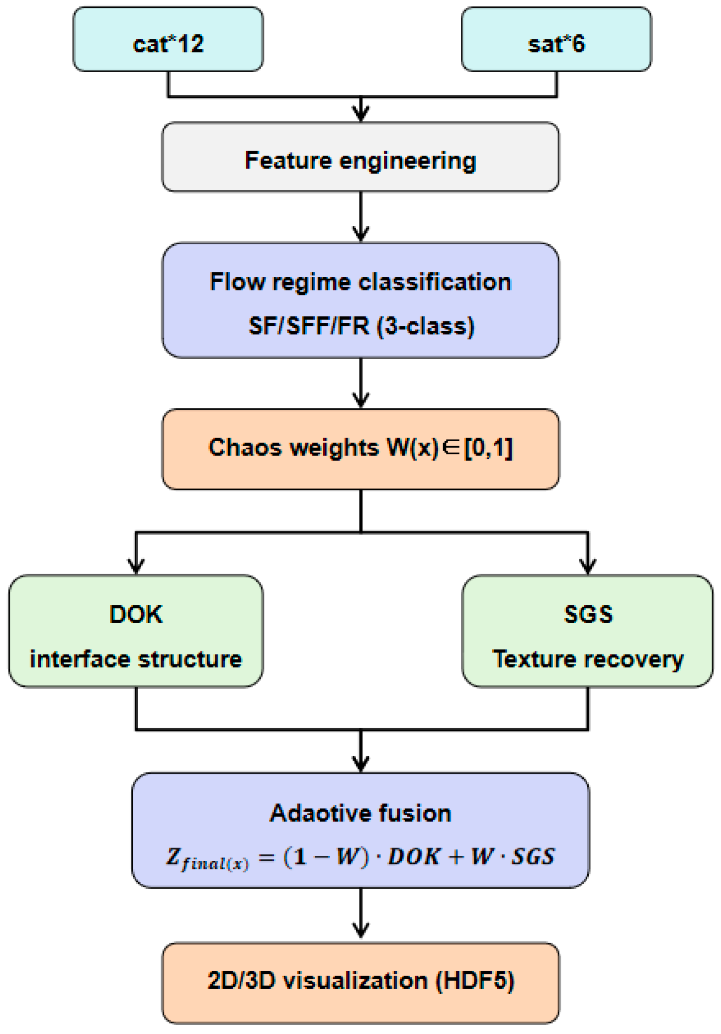
To address these issues, this paper proposes a Flow-Regime-driven Framework for Adaptive Cross-sectional Imaging (FR-FACI), which couples the identification of flow regimes with image reconstruction in a closed-loop process (see Figure 1). Physically meaningful features drive support vector machine (SVM)-based regime classification, and a chaos weight mechanism converts the classifier’s probabilistic output into continuous blending weights between detrended ordinary kriging (DOK) and sequential Gaussian simulation (SGS). The core contributions are: (1) the FR-FACI coupled framework, which adapts the reconstruction strategy according to the flow conditions and thus overcomes the limitations of single interpolation models; (2) the Chaos Weight continuous control mechanism, which eliminates artefacts caused by abrupt changes and whose robustness is validated through sensitivity analysis; and (3) quantitative variogram analysis across 12 conditions and three regimes, which demonstrates order-of-magnitude differences in spatial correlation structure and establishes the physical necessity of dual-path reconstruction.

2. Experimental System and Data Acquisition

2.1. Multiphase Flow Experimental Setup

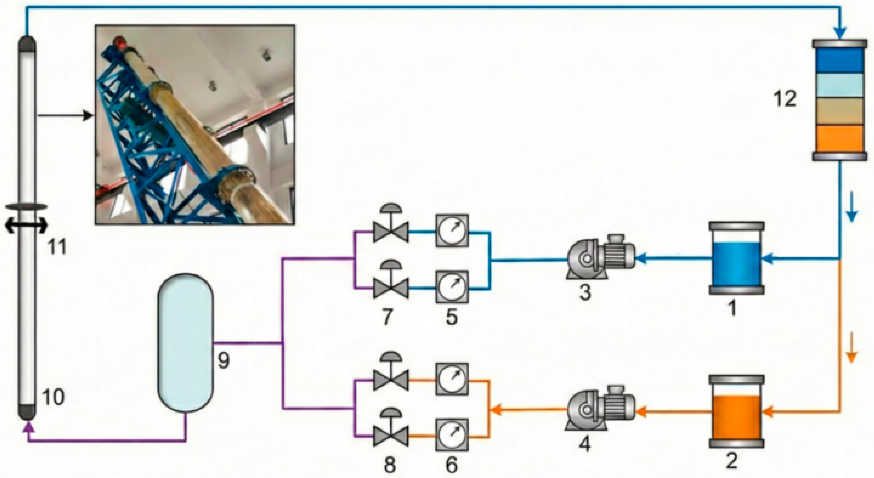
The experimental data were collected at the horizontal-well multiphase-flow simulation facility of the Ministry of Education Key Laboratory of Oil and Gas Resources and Exploration Technology at Yangtze University [2,9]. The test section of this configuration consists of a horizontal pipe with an internal diameter of 124 mm. The main body comprises a 10-metre-long transparent glass tube, facilitating visual observation of flow patterns and high-speed photographic recording. A stainless steel section, measuring one metre in length, is attached to each extremity with the objective of stabilising the flow regime. The experimental working fluids comprised No. 10 industrial white oil (density 0.826 g/cm³, viscosity 2.92 mPa·s, surface tension 30.00 mN/m) and tap water (density 0.988 g/cm³, viscosity 1.16 mPa·s, surface tension 72.00 mN/m). The oil and water phases were stored in separate tanks with flow rates regulated by PID-controlled pumps; a gravity separation tank (residence time > 30 min) ensured complete phase segregation and fluid reproducibility. The experimental flow circuit is shown schematically in Figure 2.

2.2. Array Sensor System

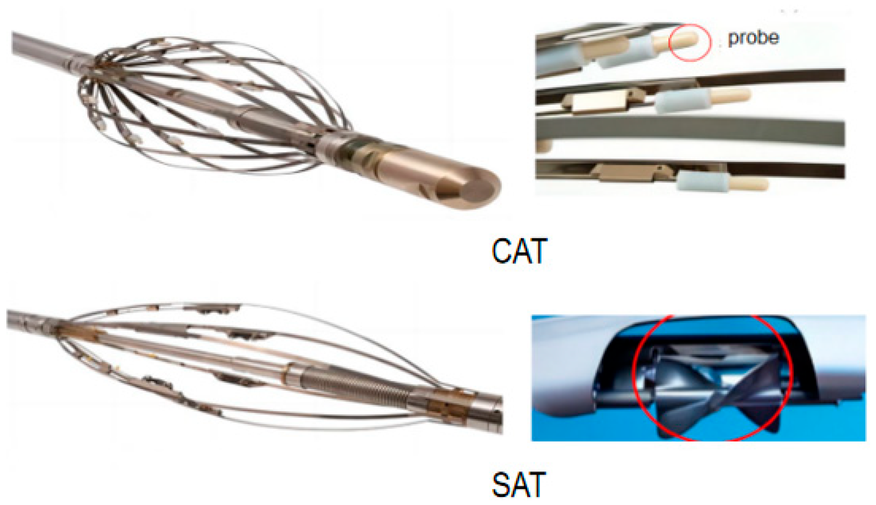
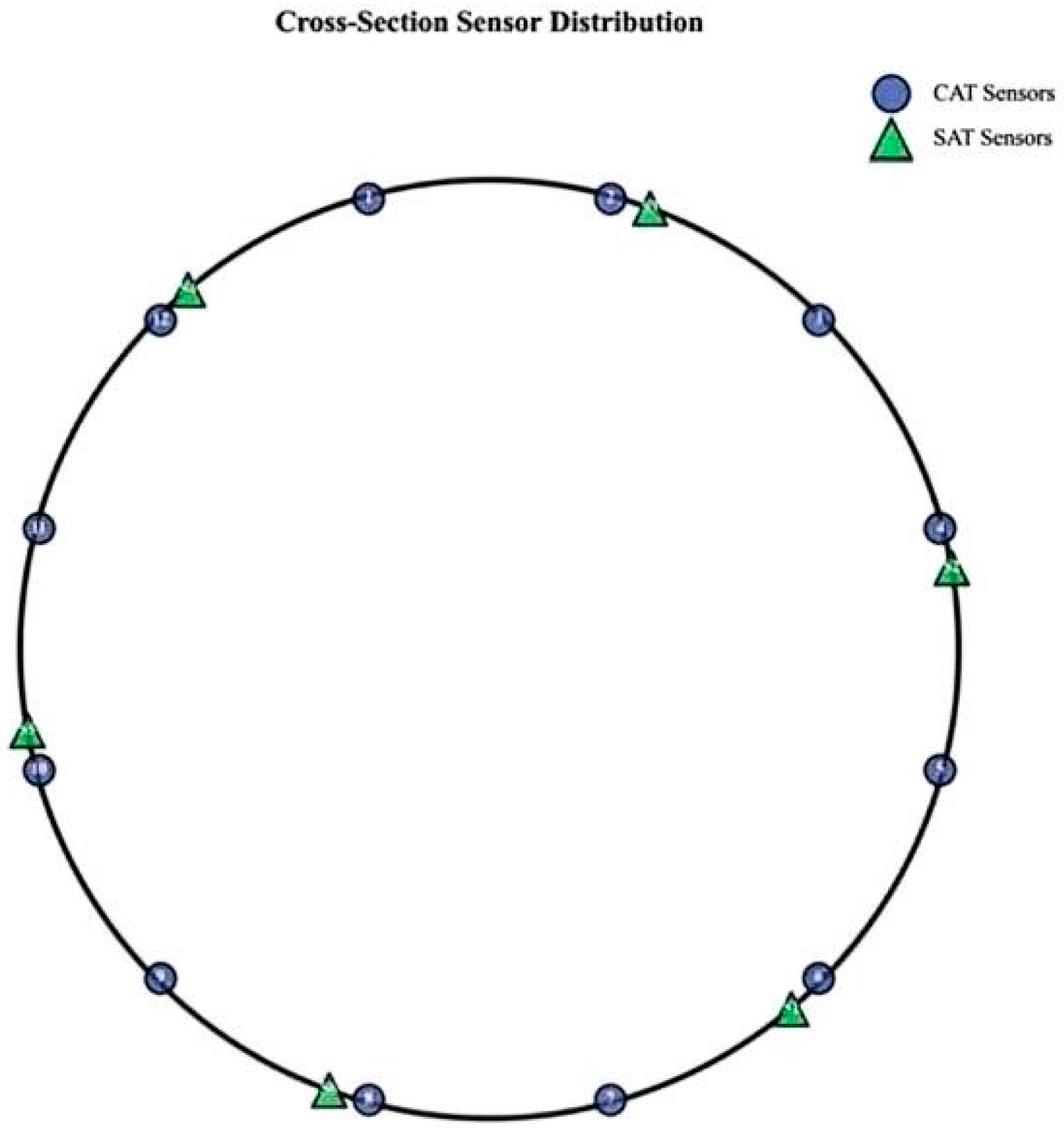
The experiment employed a Capacitance Array Tool (CAT) and a Screw Array Tachometer (SAT), whose structure and operating principles are illustrated in Figure 3. The CAT identifies oil and water phases by measuring the dielectric constant of the surrounding fluid. Each of its 12 capacitive sensors produces a frequency response proportional to the local dielectric constant: the water phase (ε ≈ 80) yields a high response (≈0.95), while the oil phase (ε ≈ 2.2) produces a moderate response (≈0.87). The SAT captures the cross-sectional velocity distribution; each turbine’s rotational speed, proportional to local fluid velocity, is converted into a frequency signal via a Hall-effect detector. The spatial distribution of all 18 sampling points is shown in Figure 4.

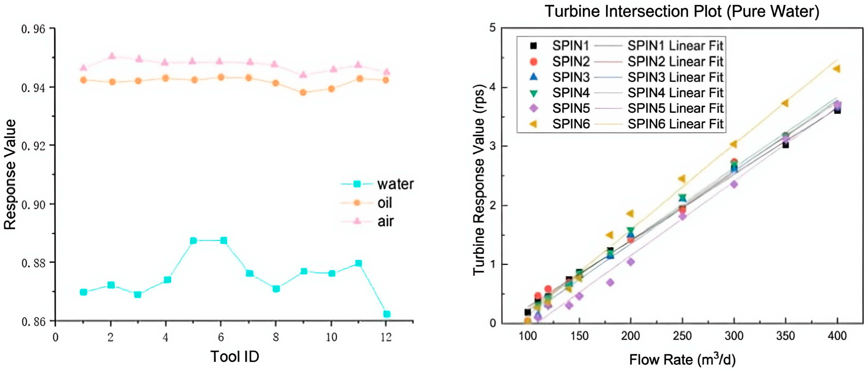
All sensors were calibrated under controlled single-phase conditions prior to experimentation (Figure 5). For the CAT, 12 probes had response values of 0.94–0.96 in pure water and 0.86–0.88 in pure oil. Their uniformity ensures negligible inter-sensor variation relative to the oil–water response contrast. For the SAT, the rotational speeds of six turbines (SPIN 1–SPIN 6) exhibit a strong linear relationship with total flow rate (R² > 0.99 for all channels), and the standard error of linear fit residuals is <2% of full-scale reading across the test flow range.

2.3. Design of Experimental Conditions and Flow Pattern Classification

The experiment was designed to create 12 sets of experimental conditions under horizontal well conditions, covering various combinations of flow rates and water cut, with the aim of capturing as many typical flow patterns of oil–water two-phase flow in horizontal wells as possible. This was achieved by systematically adjusting the oil and water flow rates. The specific parameters for each condition and the corresponding flow patterns are illustrated in Figure 1.

The 150 data sets recorded in

Table 1. Experimental Conditions and Flow Pattern Classification for Horizontal Well Oil–Water Two-Phase Flow.

No.	Total Flow Rate Q (${\mathbf{m}}^3/\mathbf{d}$)	Water Cut ${\mathit{C}}_{\mathit{w}}$ (%)	Flow Pattern	Interface Characteristics	Data Sets
1	100	20	SW	Wavy interface, minor oil entrainment	150
2	100	40	SW	Wavy interface, minor oil entrainment	150
3	100	60	ST	Smooth, stable horizontal interface	150
4	100	90	ST	Smooth, stable horizontal interface	150
5	300	20	SFF	Discernible interface, localised foaming	150
6	300	40	SFF	Discernible interface, localised foaming	150
7	300	60	SFF	Discernible interface, localised foaming	150
8	300	90	SFF	Discernible interface, localised foaming	150
9	600	20	FR	Fully disrupted, emulsified mixture	150
10	600	40	FR	Fully disrupted, emulsified mixture	150
11	600	60	FR	Fully disrupted, emulsified mixture	150
12	600	90	FR	Fully disrupted, emulsified mixture	150

represent the raw sampling points at each depth under a single operating condition. To extract statistically robust features and suppress transient noise, the raw signals were segmented using non-overlapping windows with a length of 25 and a step size of 25. This results in six window-level samples per operating condition, for a total of 72 samples across all conditions used to train and evaluate the flow pattern classifier.

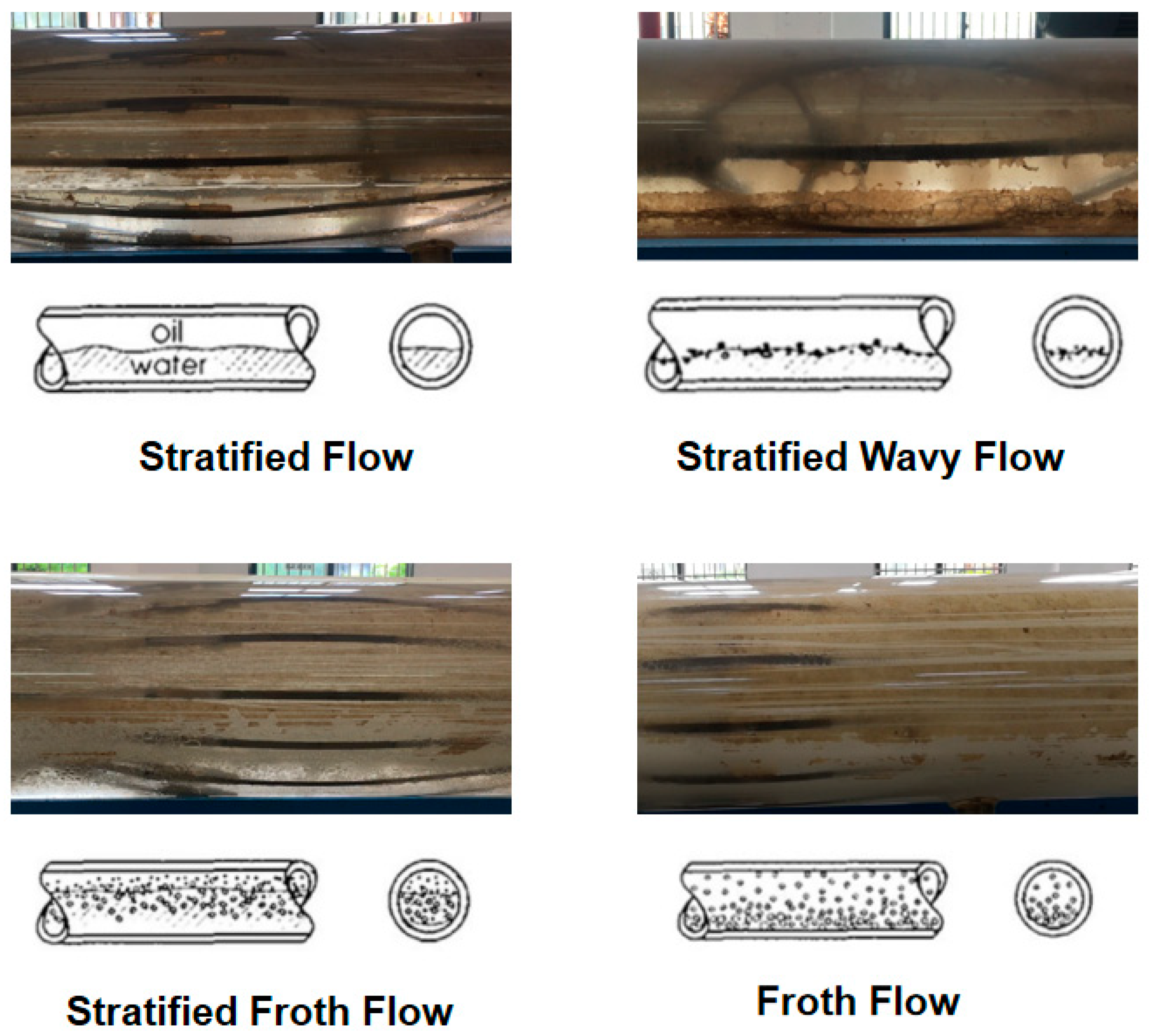
Flow pattern annotations for each operating condition were based on visual observations within the transparent pipe section and synchronised camera recordings. Within the flow rate and water cut range of this experiment, four typical flow patterns were observed; the experimental flow pattern diagram is shown in Figure 6.

Stratified Flow (ST): The flow of oil and water occurs in distinct layers that are separated by a clear horizontal interface. This interface is characterised by smoothness, with no significant disturbances, and the phase distribution within the cross-section is stable.

Stratified Wavy Flow (SW): The mixture of oil and water remains stratified, but the interface exhibits regular, small-amplitude undulations. A few oil bubbles are present at the interface, and the flow remains predominantly gravity-driven.

Stratified Froth Flow (SFF): The oil–water interface remains discernible, but there is significant entrainment of oil and water at the interface and localised foaming. The cross-section retains the overall stratified structure whilst also exhibiting significant localised mixing zones.

Froth Flow (FR): Turbulent energy has been shown to be sufficient to disrupt the phase interface completely; oil and water mix to form an emulsified frothy mass, exhibiting a disordered, patchy distribution within the cross-section.

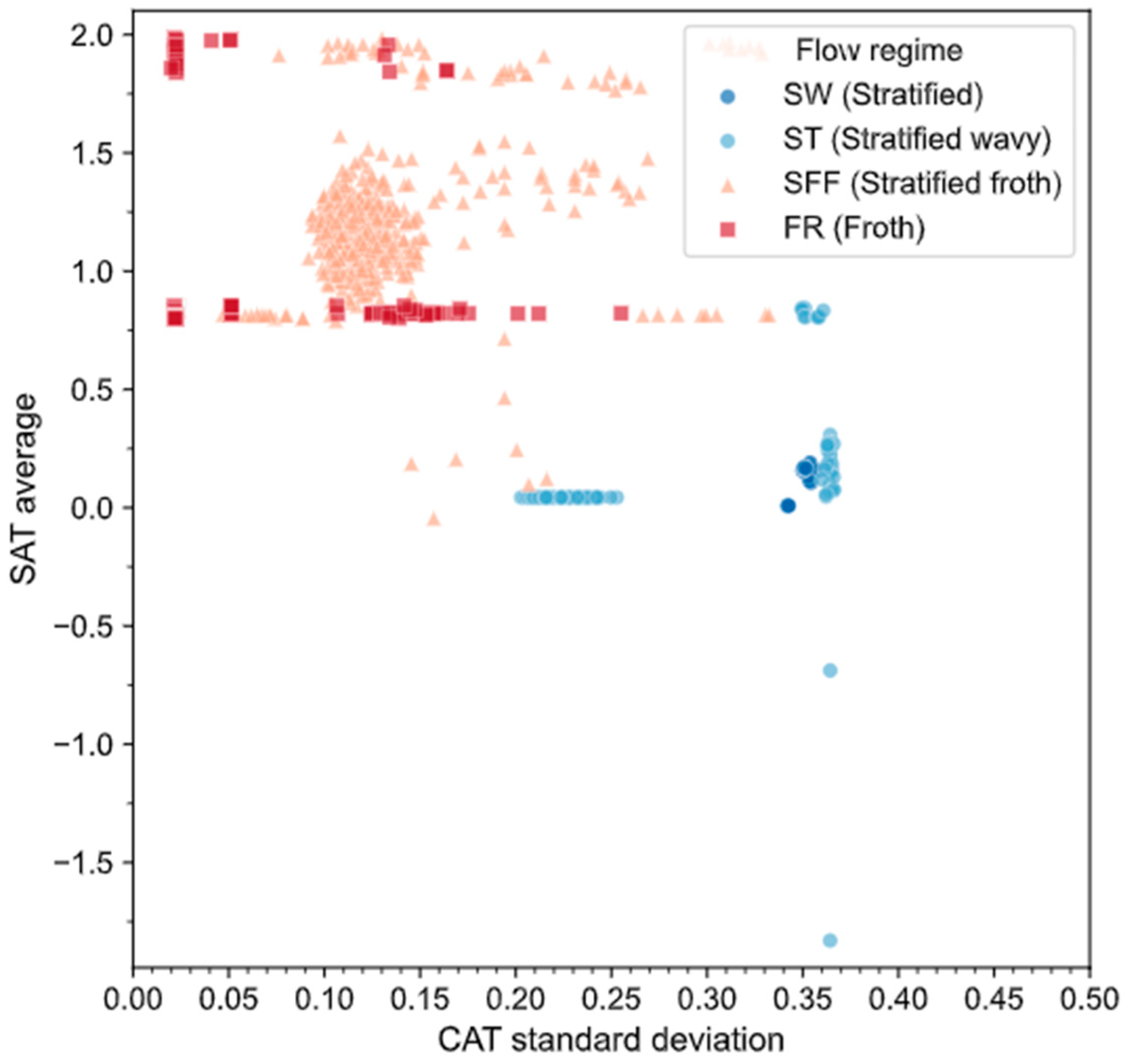
Although four flow patterns were visually identified (ST, SW, SFF, and FR), the CAT and SAT signals cannot distinguish between ST and SW. As illustrated in Figure 7, the feature-space points for ST and SW overlap significantly, whereas SFF and FR occupy distinct regions. Statistical tests (t-test or Mann–Whitney U, $\mathsf{\alpha }$ = 0.05) on all six features (

Table 2. Statistical Comparison of the Distribution of ST and SW Flow Patterns.

Feature	Test	p-Value	Cohen’s d	Conclusion
sat_overall_r2	Mann-Whitney U	0.289	0.12	Hard to distinguish
sat_nonlinear	t-test	0.184	0.19	Hard to distinguish
sat_nonlinear_ratio	Mann-Whitney U	0.512	0.08	Hard to distinguish
cat_cross_mean_var	t-test	0.685	0.05	Hard to distinguish
cat_cross_max_var	Mann–Whitney U	0.379	0.16	Hard to distinguish
cat_cross_std_var	t-test	0.032	0.46	Slightly distinguishable

) confirm that five of the six features have p > 0.05 and negligible effect sizes (Cohen’s d = 0.05–0.19). Only cat_cross_std_var reaches marginal significance (p = 0.032, d = 0.46), which is insufficient for a stable classification boundary under leave-one-condition-out validation. This merging is consistent with the findings of Torres et al. [6]. Accordingly, the algorithm uses three labels—SF, SFF and FR—for all subsequent analysis.

3. Methodology

3.1. Physics-Informed Feature Extraction and Importance Analysis

Six features are extracted from each depth sample. From the 12-channel CAT signals: CAT_mean (arithmetic mean of 12 probe readings, reflecting the overall water content level—higher values indicate water-dominated cross-sections) and CAT_std (standard deviation across probes, capturing oil–water spatial heterogeneity; in stratified flow, the bimodal oil/water distribution yields high CAT_std, while in froth flow, rapid phase alternation at each probe also elevates CAT_std, though the underlying physical mechanisms differ). From the six SAT signals: SAT_mean (mean rotational speed of six micro-turbines, directly proportional to the cross-sectional average kinetic energy—significantly higher under turbulent conditions that promote froth formation) and SAT_std (velocity non-uniformity across the cross-section, most pronounced in the vortex regions of froth flow). Two geostatistical features are computed from the experimental variogram: Range (the distance at which spatial autocorrelation decays to the sill, large in stratified flow due to strong interfacial continuity, small in froth flow due to fine-scale turbulent mixing) and Nugget (the variogram intercept at zero lag, reflecting micro-scale random variation; turbulent disturbances in froth flow produce nugget values far exceeding those of stratified flow). The variogram is defined as follows:

$$\gamma (h)={\displaystyle \frac{1}{2N\left(h\right)}}{\displaystyle \sum _{i=1}^{N\left(h\right)}}{\left[z\right(x_i)-z(x_i+h\left)\right]}^2$$

(1)

where $N\left(h\right)$ is the number of data pairs at spacing h, and $Z\left(x\right)$ is the sensor reading at position x.

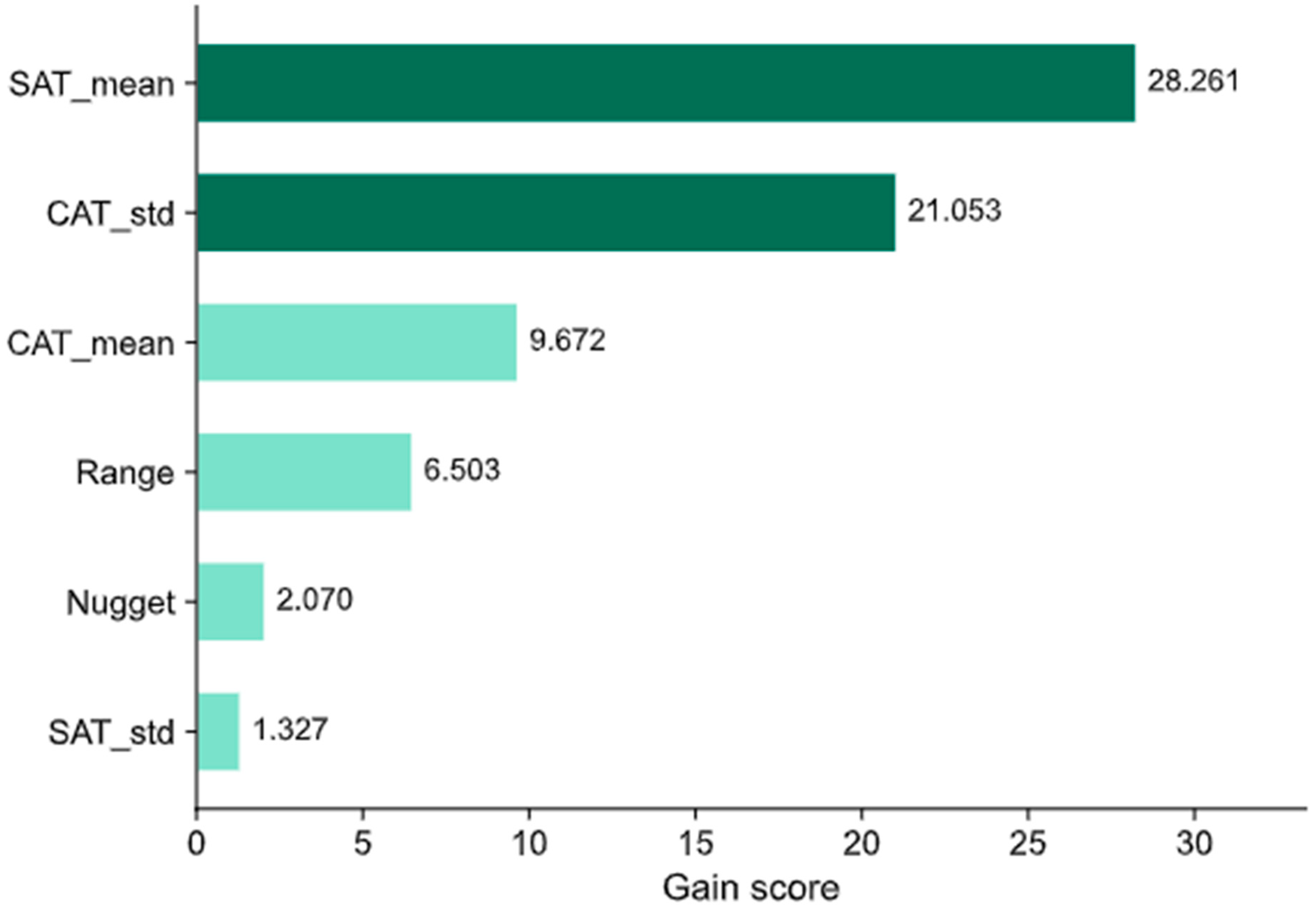
Feature importance was assessed using XGBoost (version 2.1.2) [36] gain scores (Figure 8). SAT_mean and CAT_std ranked first and second, respectively, jointly contributing ~72% of the information used for classification—consistent with the expectation that flow velocity and phase heterogeneity are the primary discriminators at a physical level. Permutation importance analysis of the SVM classifier under LOCO cross-validation (

Table 3. Permutation Feature Importance of the SVM Classifier Under LOCO Cross-Validation.

Feature	Mean Accuracy Drop (%)	Std (%)	Permutation Rank	XGBoost Gain Rank
SAT_mean	18.75	3.42	1	1
CAT_std	13.19	2.86	2	2
Range	5.56	2.14	3	4
CAT_mean	2.78	1.53	4	3
SAT_std	1.39	1.18	5	6
Nugget	0.56	0.83	6	5

) confirms this ranking, with respective accuracy drops of 18.75% and 13.19% for these two features. The remaining four features provide supplementary, albeit progressively smaller, contributions.

3.2. Chaos Weight Mechanism: From Discrete Classification to Continuous Imaging Control

3.2.1. Classifier Training and Model Selection

Based on the features selected in Section 3.1, three classifiers representing distinct learning paradigms were compared for flow-type discrimination among SF, SFF, and FR: (i) SVM [37] with an RBF kernel (C = 10, γ = scale, balanced class weights), chosen for its margin-based regularisation and suitability for small-sample problems; (ii) logistic regression (LogReg) as a linear baseline, whose softmax output provides inherently calibrated probabilities; and (iii) XGBoost (n_estimators = 80, max_depth = 2, learning_rate = 0.05), representing gradient-boosted ensemble learning with hyperparameters tuned to avoid overfitting on the limited training set.

Generalisation was evaluated using leave-one-condition-out (LOCO) cross-validation: in each of 12 iterations, all data from one operating condition were held out for testing while the model was trained on the remaining 11 conditions. This is more rigorous than random splitting, as the model must generalise to an entirely unseen operating condition. Classification results are reported in Section 4.1.

3.2.2. Chaos Weight Generation

Beyond providing a discrete label, the classifier outputs probability estimates for each class, which are used for continuous imaging control.

In this paper, Platt Scaling [38] is employed to transform the raw decision values into class probabilities. In the context of a three-class classification scenario, this results in the generation of probability vectors for SF, SFF, and FR, with the proviso that the sum of these vectors is equivalent to 1.

$$p(x)={\left[P\right(SF\left|F_X\right),P\left(SFF\right|F_X),P(FR\left|F_X\right)]}^T,\sum _k{p}_k\left(x\right)=1$$

(2)

where ${\mathrm{F}}_{\mathrm{x}}$ is the feature vector at position x. Calibration is performed using 5-fold internal cross-validation within each LOCO training fold to avoid information leakage.

The quality of calibration is evaluated using two metrics: the Brier Score and the expected calibration error. The Brier Score (BS) quantifies the discrepancy between predicted probabilities and true labels; lower values indicate superior calibration. The expected calibration error (ECE) is a metric used to assess the congruence between the predicted confidence levels and the actual classification accuracy. A lower value is generally considered more favourable. As demonstrated in

Table 4. Probability calibration metrics under LOCO cross-validation.

Model	Multi-Class BS	BS (SF)	ECE (SF)	BS (SFF)	ECE (SFF)	BS (FR)	ECE (FR)
SVM	0.113	0.029	0.105	0.054	0.129	0.031	0.089
XGBoost	0.163	0.059	0.077	0.054	0.097	0.050	0.147

, the SVM employing Platt Scaling achieved a lower multi-class Brier Score and an inferior ECE for the FR class compared to XGBoost. As the chaotic weights are directly defined as P(FR), the SVM’s low BS (0.031) and ECE (0.089) for FR confirm that the calibrated probabilities are sufficiently reliable and can be used as weights for continuous imaging control.

The chaos weight W(x) is defined as the classifier’s predicted probability of the foam flow category:

$$W\left(x\right)=P\left(FR\right|F_x)$$

(3)

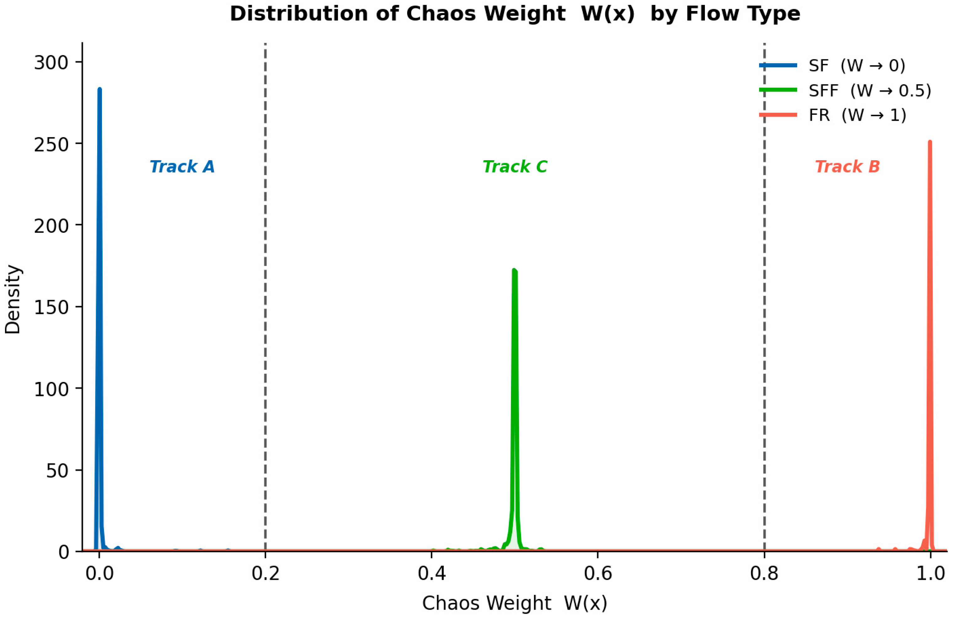
As a continuous measure of the intensity of local flow chaos, W(x) has a direct correspondence with the spatial statistical structure of the cross-sectional field. When W(x) approaches zero, the classifier reliably identifies laminar flow, and the cross-sectional field manifests a smooth structure with a discernible interface. Conversely, when W(x) approaches one, the classifier reliably identifies foamy flow, and the cross-sectional field should be chaotic, characterised by a complex, foamy texture. As illustrated in Figure 9, the empirical distribution of W(x) under the three flow regimes is as follows: under SF conditions, W(x) is tightly concentrated around 0; under FR conditions, it is concentrated around 1; and under SFF conditions, the distribution centre is approximately at 0.5. The weights are not uniformly distributed between 0 and 1 but cluster into three distinct bands—low, medium, and high—corresponding to the three flow regimes. The tight intra-regime clustering and clear inter-regime separation confirm that the Platt-calibrated SVM probabilities provide reliable continuous control signals for adaptive reconstruction.

3.3. Dual-Path Adaptive Reconstruction

3.3.1. Path A: Detrended Ordinary Kriging (DOK)—For Stable Stratified Flow

In laminar flow conditions, gravity-driven oil–water separation leads to a systematic vertical gradient in the water content field across the cross-section, from the top of the pipe (pure oil) to the bottom (pure water). This results in a violation of the assumption of intrinsic stationarity, which is a prerequisite for the application of ordinary Kriging [39]. For this reason, the present study employs detrended ordinary Kriging (DOK), a methodology which decomposes the water content field into a deterministic trend component and a stochastic residual component:

$$Z\left(x\right)=m\left(y\right)+R\left(x\right)$$

(4)

where $\mathrm{m}\left(\mathrm{y}\right)$ is the large-scale trend function related to the vertical position $y$, and $R\left(x\right)$ is the random residual after detrending, assumed to satisfy the assumption of internal stationarity. The trend (y) is estimated by fitting a regression of sensor readings on their vertical coordinates; in stratified flow, the vertical trend can typically be described by an S-shaped function or a polynomial approximation.

After trend removal, the residual $\mathrm{R}\left(x\right)=Z\left(x\right)-m\left(y\right)$ is modelled using a variogram function and ordinary Kriging interpolation. The ordinary Kriging of the residual is:

$${\widehat{R}}^{*}(x_0)={\displaystyle \sum _{i=1}^n}{\lambda }_{i}R(x_i)$$

(5)

where ${\mathsf{\lambda }}_{\mathrm{i}}$ is the Kriging weight, obtained by solving the following system of equations:

$$\left\{\begin{array}{c}{\sum }_{j=1}^n{\lambda }_i\gamma (x_i-x_j)+\mu =\gamma \left(x_{i-}{x}_0\right),i=1,\dots ,n\hfill \\ {\sum }_{i=1}^n{\lambda }_i=1\hfill \end{array}\right.$$

(6)

where $\mathsf{\lambda }(·)$ is the theoretical fitting model of the experimental variance function of the residuals, and $\mathsf{\mu }$ is the Lagrangian multiplier. The final reconstructed value is:

$$Z_A^{*}(x_0)=m(y_0)+{\widehat{R}}^{*}(x_0)$$

(7)

The advantage of DOK lies in its ability to transform a non-stationary problem into a stationary one by removing trends, thereby ensuring that Kriging satisfies the Best Linear Unbiased Estimation property [39,40]. Its output is deterministic and smooth, capable of precisely preserving the spatial continuity of the oil–water interface in stratified flow. However, this very smoothness constitutes its shortcoming in chaotic flow patterns, as it systematically flattens the high-frequency texture of foam flow.

3.3.2. Path B: Sequential Gaussian Simulation (SGS)—For Chaotic Froth Flow

In conditions of foaming flow, the turbulent energy disrupts the phase interface, resulting in the mixing of oil and water in the form of disordered, small-scale patches. This process leads to high-frequency spatial variations in the cross-sectional field. The use of Kriging to achieve a smoothing effect is an effective method of preventing the reproduction of chaotic textures [19]. In order to recover the high-frequency information that is typically lost by deterministic methods, this study employs Sequential Gaussian Simulation (SGS) [20] for the foaming flow path.

SGS is a conditional random simulation method whose core principle involves introducing random perturbations that obey the Kriging variance onto the Kriging mean. This ensures that the generated realisations statistically retain the same histogram and variogram structure as the original data [22]. The process commences with the conversion of the original water content values to a standard normal distribution via quantile mapping. Subsequently, a random access sequence is generated on the simulation grid. At each unvisited node, simple Kriging is performed using the k nearest available data points (k = min(10, n_available)) to obtain the conditional mean and variance. From these, a value is randomly sampled and added to the conditional data set. Once all nodes have been visited, the simulated field is transformed back to the original data space.

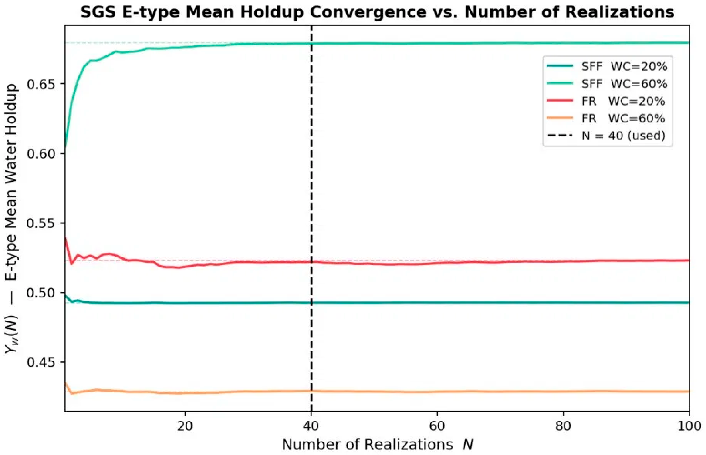
In this study, the standard SGS process was appropriately modified to suit the requirements of cross-sectional imaging. Initially, 40 independent runs were generated for each cross-section, and the ensemble mean was then employed as the final estimate ${\mathrm{Z}}_{\mathrm{B}}^{*}(\mathrm{x})$ to suppress node-level noise from individual runs whilst retaining statistical texture. This number was validated through a convergence analysis (Figure 10): the E-type mean holdup Yw(N) stabilises before N = 20 for all tested SFF and FR conditions, with a maximum absolute deviation of 0.0011 relative to the N = 100 reference—well within a 0.5% tolerance. The SF regime is excluded because the Chaos Weight effectively nullifies the SGS contribution (W < 0.02). The variance between runs was utilised as an estimate of prediction uncertainty. Secondly, given the potential instability of the experimental variance function fitting process under chaotic flow conditions, the SGS path fitting range is constrained within a physically reasonable interval. This is done to prevent the emergence of long-range correlation structures that are inconsistent with small-scale turbulent flow. Furthermore, a texture boost parameter is introduced to control the amplitude of random perturbations, with FR set to 2.0 and SFF set to 1.5 to match the differences in the intensity of high-frequency spatial variability across different flow regimes. These operational values were selected based on the sensitivity analysis in Section 4.4, where boost values from 0.5 to 4.0 were tested. Higher values (b = 4.0) served only to probe the imaging response at extreme perturbation amplitudes and were not used in the final reconstruction. It has been demonstrated that, given the chaotic weight suppresses W(x) to near zero in the laminar region, the contribution of the SGS path is automatically suppressed. Consequently, the setting of the boost parameters has virtually no effect on the laminar imaging results, thereby reducing the engineering burden of parameter tuning for each flow regime. The sensitivity of imaging quality to the boost parameters is analysed in Section 4.4.

3.3.3. Adaptive Fusion

The final cross-section reconstruction is achieved by adaptively fusing the outputs of the two paths via chaotic weights:

$$Z_{final}\left(x\right)=(1-W(x\left)\right)·Z_A^{*}\left(x\right)+W\left(x\right)·Z_B^{*}\left(x\right)$$

(8)

where ${\mathrm{Z}}_{\mathrm{A}}^{*}(\mathrm{x})$ is the output of the DOK path, ${\mathrm{Z}}_{\mathrm{B}}^{*}(\mathrm{x})$ is the output of the SGS path, and $\mathrm{W}\left(\mathrm{x}\right)\in [0,1]$ is the chaotic weight. The physical interpretation of this formula is that in the laminar flow region, the weight approaches zero, and the output is almost entirely controlled by DOK, maintaining a smooth interface; in the turbulent region, the weight approaches one, and the output is almost entirely controlled by SGS, restoring the turbulent texture; in the transition region, the two paths are smoothly blended probabilistically, avoiding spatial discontinuities caused by abrupt switching.

The variance of the fusion output can be decomposed as follows:

$${\sigma }_{final}^2(x)={[1-W(x\left)\right]}^2·{\sigma }_{DOK}^2(x)+{W\left(x\right)}^2·{\sigma }_{SGS}^2(x)+W(x)[1-W(x)]·{\left[Z_A^{*}\right(x)-Z_B^{*}(x\left)\right]}^2$$

(9)

The first two terms represent the weighted variances of the two paths respectively, whilst the third term reflects the divergence between DOK and SGS. When W(x) approaches 0.5, and the two paths yield significantly different predictions—at which point this term is maximised—the flow type is in a transitional state (SFF).

Furthermore, to ensure the physical consistency of the reconstruction results, a boundary constraint is applied to the blended output:

$$Z_{final}\left(x\right)=max(0,min(1,Z_{final}\left(x\right)\left)\right)$$

(10)

This strictly confines the reconstructed moisture content values to the interval [0, 1], thereby avoiding unreasonable phenomena such as negative moisture content or supersaturation.

3.3.4. Comparative Method: Gaussian Process Regression (GPR)

To assess whether optimising the interpolation model alone can match FR-FACI, Gaussian process regression (GPR) is included as a single-model benchmark. GPR shares Kriging’s Gaussian-process foundation, but replaces manual variogram fitting with automatic kernel hyperparameter optimisation via log-marginal likelihood. This reduces subjectivity in sparse-data settings [28,29]. A Matérn kernel (ν = 2.5) combined with constant and white-noise kernels was used, with all hyperparameters optimised by L-BFGS-B. Hyperparameter optimisation was performed independently for each cross-section within the leave-one-sensor-out framework, where the Matérn Iength scale, output variance, and white-noise variance were jointly determined by maximising the log-marginal likelihood over the remaining sensor readings. As with DOK, a first-order vertical trend was removed prior to interpolation.

3.4. 3D Volumetric Reconstruction and Visualization

Cross-sectional imaging provides only two-dimensional information on fluid distribution at a single depth. To construct a continuous three-dimensional visualisation along the wellbore axis, this study employs a data baking strategy to expand the two-dimensional reconstruction results at discrete depths into three-dimensional volumetric data [40,41].

$$V(x,y,z)={\displaystyle \frac{z_{k+1}-z}{z_{k+1}-z_k}}{Z}_{final}(x,y,z_k)+{\displaystyle \frac{z-z_k}{z_{k+1}-z_k}}{Z}_{final}(x,y,z_{k+1})$$

(11)

and $z_k\le z\le z_{k+1}$.

This process converts discrete two-dimensional images into continuous three-dimensional volumetric data, similar to inter-slice interpolation in medical CT imaging. The output files can be directly integrated with web-based 3D rendering engines to achieve interactive visualisation of fluid distribution within the wellbore.

4. Results and Discussion

4.1. Flow Regime Classification

As shown in

Table 5. Performance Comparison of Classifiers via Leave-One-Condition-Out (LOCO) Cross-Validation.

Classifier	Accuracy	Macro-F1	SF Precision	SF Recall	SFF Precision	SFF Recall	FR Precision	FR Recall	Acc Std
SVM	95.83%	0.958	1.00	1.00	0.889	1.00	1.00	0.875	0.138
LogReg	90.28%	0.903	0.958	0.958	0.793	0.958	1.00	0.792	0.23
XGBoost	84.72%	0.851	0.952	0.833	0.697	0.958	1.00	0.750	0.315

, the SVM achieved 95.83% overall accuracy and a Macro-F1 of 0.958 under LOCO cross-validation, outperforming both LogReg (90.28%) and XGBoost (84.72%). XGBoost exhibited the greatest variance across folds (standard deviation = 0.315), consistent with the recognised instability of greedy splitting in small-sample regimes [11]; the SVM’s margin-based decision boundary proved more robust to training-set perturbations.

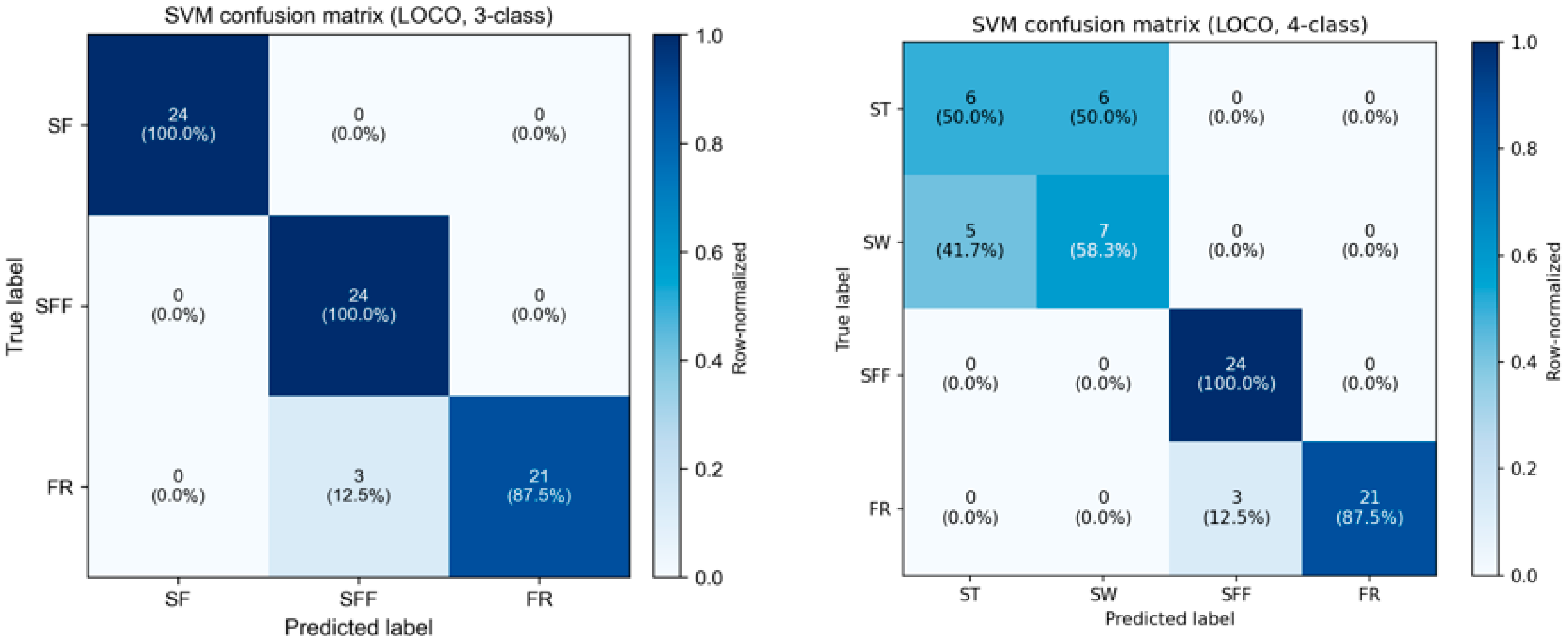
The confusion matrix (Figure 11, left) shows no misclassifications for SF and SFF, with only three out of 24 FR samples misclassified as SFF. When the original four-class labels are retained (Figure 11 on the right), ST and SW exhibit near-random cross-classification (6/12 and 5/12, respectively). This confirms that their merger into SF is both necessary and effective at the classifier level, as three-class accuracy improved from 75% to 95.83%.

4.2. Spatial Statistical Structure Across Flow Regimes

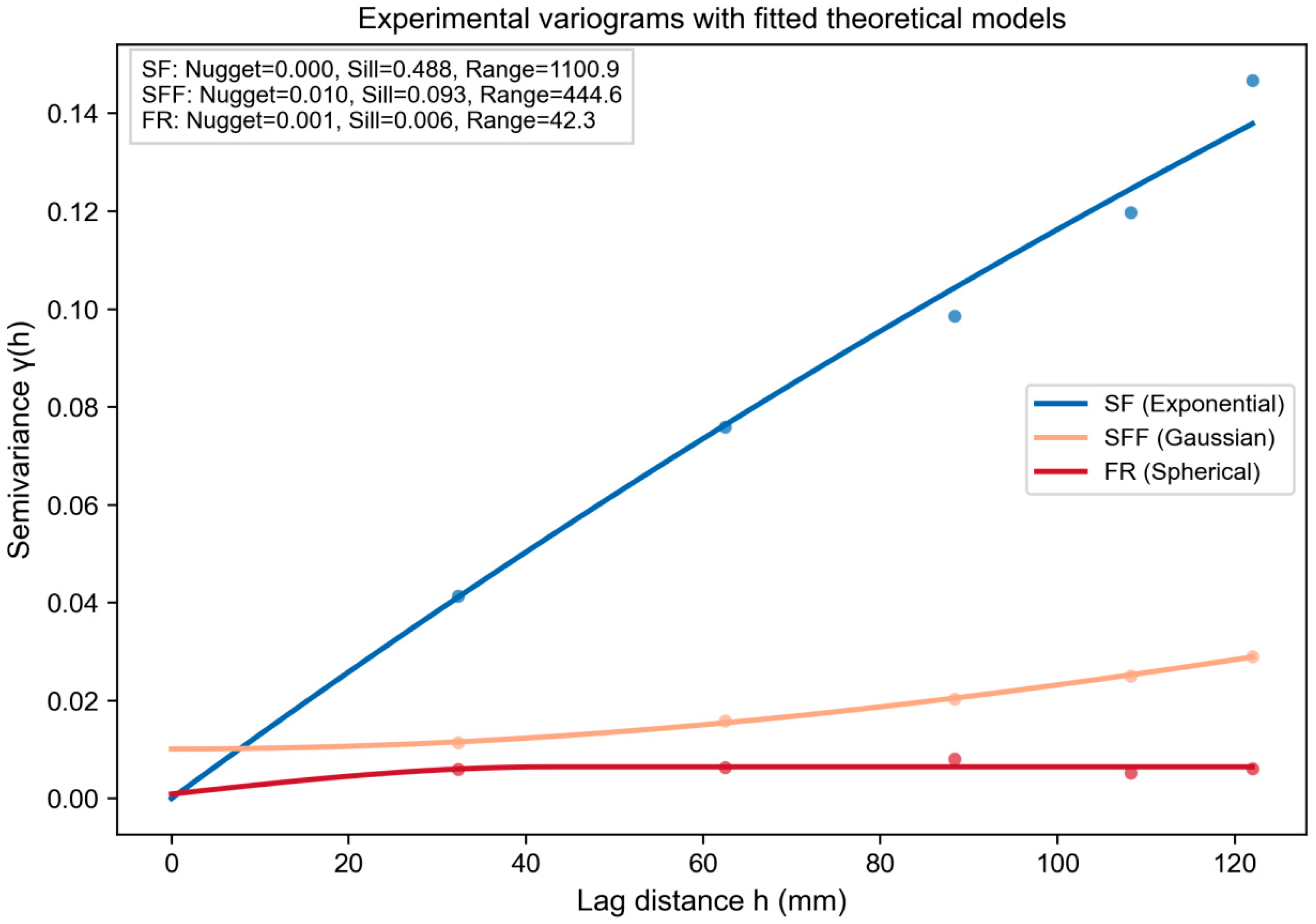
Figure 12 shows the experimental variograms and fitted models for the three regimes. The FR model reaches its sill at a lag of approximately 40 mm, the SFF model rises gradually without reaching its sill within the observation range, and the SF model continues to increase over the entire range, with a fitted range of 1100.9 mm. This 26-fold difference confirms the presence of regime-dependent spatial structure. The sill values likewise reflect the intensity of phase mixing: SF exhibits the highest sill value (0.488) due to the bimodal oil–water contrast across a sharp interface. In contrast, FR shows the lowest sill value (0.006) because turbulent mixing homogenises local readings. However, the low FR sill does not imply spatial uniformity. Rather, the characteristic scale falls below the sensor spacing—precisely the sub-resolution gap that the SGS path is designed to fill. The physical origin of these differences lies in the governing flow mechanisms. In SF, gravity dominates: the denser water phase settles to the pipe bottom, producing a stable, continuous interface whose spatial correlation extends over distances comparable to the pipe diameter (range ≈ 9D). In FR, turbulent inertia overcomes gravitational segregation, fragmenting the oil–water interface into droplets and patches at scales governed by local energy dissipation. This confines spatial correlation to ~40 mm, consistent with the measured FR range. SFF represents the transitional regime where gravitational and inertial forces are of comparable magnitude, producing an interface that is globally discernible but locally disrupted—hence its intermediate variogram behaviour.

4.3. Cross-Sectional Imaging Performance

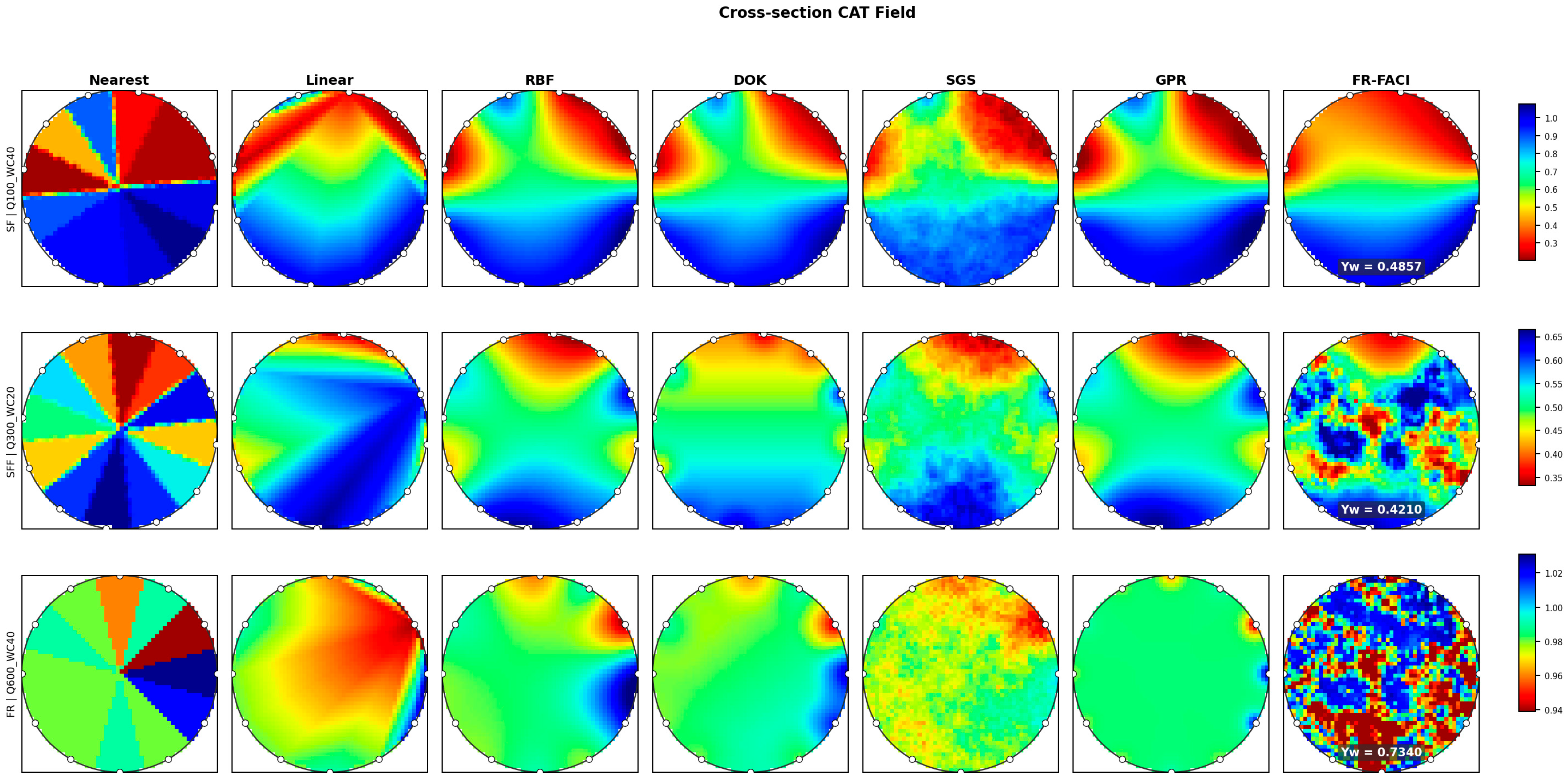
Figure 13 compares the cross-sectional images produced by seven methods under SF, SFF and FR conditions. Under SF conditions, most methods produce similar results, except for the Nearest method, which exhibits Voronoi artefacts. Differences become more pronounced with increasing flow complexity: Linear, RBF, DOK and GPR all oversmooth the interface mixing zone under SFF and FR conditions, whereas SGS recovers texture, but applies perturbations indiscriminately to all regimes. The FR-FACI method adapts according to the chaos weight. Under SF conditions (W ≈ 0), imaging is DOK-controlled. Under SFF conditions (intermediate W), interface regions exhibit localised texture, while bulk regions remain smooth. Under FR conditions (W ≈ 1), the SGS path dominates, recovering chaotic oil–water patch structures.

Table 6. Quantitative Imaging Error Comparison via Leave-One-Sensor-Out (LOSO) Cross-Validation.

Method	SF-MAE	SF-RMSE	SFF-MAE	SFF-RMSE	FR-MAE	FR-RMSE	Overall-MAE	Overall-RMSE
Nearest	0.195	0.305	0.106	0.144	0.056	0.102	0.119	0.203
Linear	0.195	0.305	0.106	0.144	0.056	0.102	0.119	0.203
RBF	0.174	0.220	0.103	0.137	0.069	0.113	0.115	0.163
DOK	0.168	0.232	0.091	0.120	0.069	0.095	0.105	0.160
SGS	0.180	0.238	0.133	0.182	0.579	0.699	0.297	0.439
GPR	0.171	0.247	0.103	0.133	0.054	0.097	0.108	0.168
FR-FACI	0.168	0.232	0.091	0.120	0.056	0.094	0.105	0.160

quantifies the LOSO cross-validation errors. DOK and FR-FACI both achieve the lowest overall mean absolute error (MAE) (0.105) and root mean square error (RMSE) (0.160). Under FR conditions, the MAE of FR-FACI (0.056) is lower than that of DOK (0.069), indicating that the SGS path recovers texture while reducing pointwise error. GPR achieves an overall MAE of 0.108 and the lowest FR-MAE (0.054), which confirms the flexibility of hyperparameters based on data. However, as a single model, it cannot match the performance of FR-FACI in adapting to different regimes. Unconstrained SGS shows severe bias (FR-MAE = 0.579), which highlights the importance of regulating the Chaos Weight.

4.4. SGS Boost Parameter Sensitivity

The theoretical quality of FR-FACI is contingent not only on the path selection process, but also on the influence of the texture enhancement parameter (boost) within the SGS path. The boost functions to regulate the amplitude of random perturbations; if the boost is insufficient, texture recovery is inadequate, whilst if the boost is excessive, this results in the introduction of unnecessary noise. The SF operating condition corresponds to track A (W < 0.2), which uses a pure DOK path and does not involve the SGS step. Therefore, the boost parameter is ineffective in this case, and the selection of boost is relevant only to SFF and FR.

Table 7. The Effect of SGS Boost Parameters on Imaging Errors under SFF and FR Conditions.

Boost	SFF Mean $\left|∆{\mathit{Y}}_{\mathit{w}}\right|$	SFF Max $\left|∆{\mathit{Y}}_{\mathit{w}}\right|$	FR Mean $\left|∆{\mathit{Y}}_{\mathit{w}}\right|$	FR Max $\left|∆{\mathit{Y}}_{\mathit{w}}\right|$
0.5	0.057	0.099	0.146	0.187
1.0	0.061	0.108	0.144	0.187
1.5	0.060	0.106	0.144	0.189
2.0	0.057	0.100	0.136	0.183
2.5	0.054	0.095	0.130	0.181
3.0	0.051	0.089	0.125	0.180
3.5	0.051	0.088	0.129	0.179
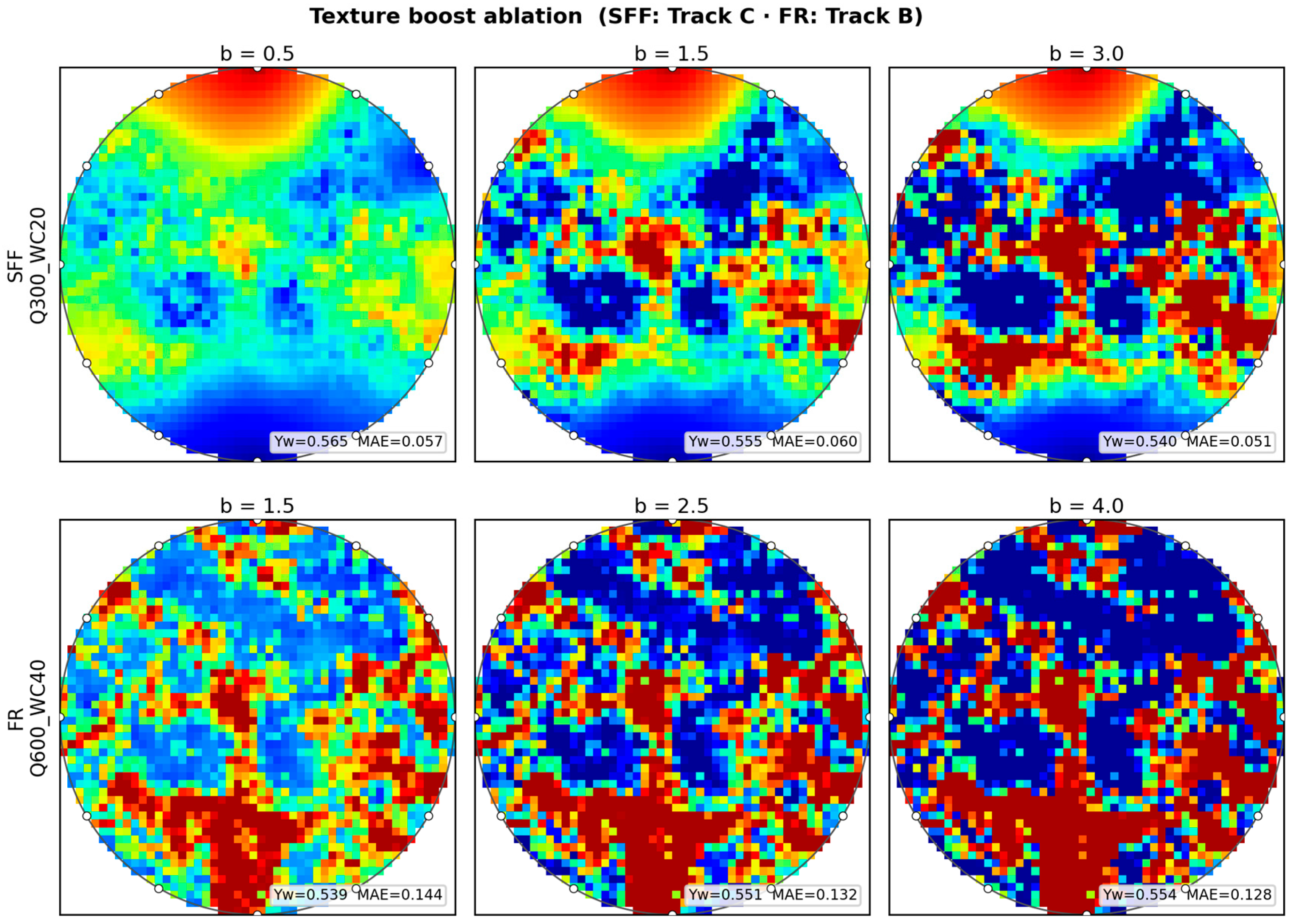
4.0	0.053	0.092	0.128	0.179

presents the mean and maximum values of the $\left|∆Y_w\right|$ for SFF and FR under various levels of boost. The error for FR tends to level off after b = 2.0, with only a 0.008 improvement from b = 2.0 to 4.0, whilst the error for SFF continues to decrease as the boost increases. However, MAE measures the average deviation in water content across the cross-section; it is insensitive to spatial texture, and under high boost levels, physical boundary constraints truncate extreme-value pixels, causing a spurious pull-back in the mean. Consequently, it cannot be regarded as the exclusive foundation for selection.

Combined with a visual assessment of the cross-sectional images, the SFF begins to reveal the texture of the interface mixing zone at b = 1.5 without a significant increase in error; however, at b ≥ 2.0, the texture becomes too pronounced, obscuring the underlying layered structure. For FR, the moisture content colour gradient transition is complete at b = 2.0; however, when b ≥ 3.0, the intermediate transition colours disappear, and the pixel-level discontinuities (approximately 2.5 mm per pixel) do not match the droplet scale of the foam flow, which ranges from a few millimetres to a few centimetres. The selection of SFF was made with a value of b set at 1.5, whilst that of FR was set at 2.0.

As demonstrated in Figure 14, even when the global boost is set to 3.0, the imaging under SF conditions remains smooth. The Chaos Weight in the SF region has been demonstrated to suppress W(x) to a negligible level, thereby effectively isolating the contribution of the SGS path. This, in turn, serves to reduce the engineering burden associated with the fine-tuning of parameters on a per-flow basis. The boost values were selected using a two-criterion procedure: first, identifying the MAE plateau point beyond which further increases yield diminishing error reduction (<0.01 in mean ΔYw); second, verifying through visual assessment that the reconstructed texture scale remains physically consistent with the expected droplet or mixing-zone dimensions for each regime. This semi-quantitative approach was adopted because no independent high-resolution ground truth (e.g., ECT cross-sectional imaging) was available to define an objective texture-fidelity metric. The boost values used throughout Section 4.3 and Section 4.6 are 1.5 for SFF and 2.0 for FR.

4.5. Uncertainty and Generalisability

FR-FACI provides a natural uncertainty estimate through the fusion variance defined in Equation (9). The DOK path contributes the Kriging variance ${\sigma }_{DOK}^2$, while the SGS path provides the inter-realisation variance ${\sigma }_{SGS}^2$ derived from the 40-run ensemble. The first two terms of that expression, ${[1-W(x\left)\right]}^2·{\sigma }_{DOK}$ and ${W\left(x\right)}^2·{\sigma }_{SGS}$, represent the weighted prediction variances of the DOK and SGS paths, respectively. The third term, $\mathrm{W}(1-\mathrm{W})·{({\mathrm{Z}}_{\mathrm{A}}-{\mathrm{Z}}_{\mathrm{B}})}^2$, captures the divergence between the two paths. This term reaches its maximum at W ≈ 0.5, which is typical of the SFF transition zone. It accordingly highlights regions with the greatest reconstruction ambiguity. Even so, the current framework fails to propagate such pixel-level variance to derived quantities including volumetric water holdup and three-dimensional fields. Rigorous uncertainty propagation can be implemented by performing Monte Carlo sampling on classifier probability and SGS realisations. This approach can deliver confidence intervals for integrated production parameters and merits further investigation in future research.

The SVM classification process is estimated to require approximately 0.15 milliseconds per window, while the DOK interpolation process takes around 5.6 milliseconds per cross-section. However, these times are considered negligible when compared with conventional logging speeds of one frame every one to two seconds. The SGS workflow necessitates a processing time of 66 s per cross-section when generating 40 realisations, and this has become the primary computational bottleneck due to its sequential Python -3.14 loop structure. Compiled inner loops and multi-core parallelisation of independent realisations are expected to reduce this cost substantially.

The current validation covers three flow regimes in a 124 mm horizontal pipe. Two aspects of generalisability warrant discussion. First, regarding transitional flow regimes: the continuous nature of the Chaos Weight inherently provides interpolation for regimes not explicitly trained, such as dispersed-droplet or annular flow. Nevertheless, extending the classifier to additional regime labels and validating the weight response across a broader regime map remain necessary before field deployment. Second, regarding pipe diameter: the variogram parameters (range, sill, nugget) are expected to scale with pipe geometry. In larger-diameter wells, the sensor spacing-to-diameter ratio decreases, potentially improving spatial resolution; however, the number and arrangement of sensors may also change, affecting the variogram structure. Transfer learning or diameter-normalised feature engineering could mitigate the need for full retraining, but experimental validation on alternative pipe sizes is required to confirm this hypothesis.

4.6. 3D Visualization and Experimental Validation

As illustrated in

Table 8. Comparison of Experimental Photographs and 3D Volumetric Imaging for Typical Flow Patterns.

Flow Patterns	Experimental Fig.	3D Imaging
SF
SFF
FR

, a comparative analysis is presented of the 3D visualisation models for the three typical operating conditions (SF, SFF and FR) alongside photographs captured during the transparent tube experiments. The SF photographs show clear oil–water stratification with a continuous horizontal interface, which the 3D model reproduces faithfully. Under SFF conditions, the model captures both the overall layered structure and the localised mixing-zone texture at the interface, reflecting the Chaos Weight’s intermediate blending of DOK and SGS paths. Under FR conditions, the characteristic ‘milky white’ chaotic appearance observed experimentally is matched by the heterogeneous oil–water patch distribution in the 3D reconstruction, with texture evolving naturally along the axial direction.

To quantify the volumetric deviation between the reconstructed field and the sensor reference, the volume deviation and relative deviation were defined as:

$${\mathsf{\delta }}_{\mathrm{v}}=Y_{w,\mathrm{r}}-Y_{w,v}$$

(12)

$$\mathrm{r}\mathrm{e}\mathrm{l}\mathrm{a}\mathrm{t}\mathrm{i}\mathrm{v}\mathrm{e}\mathrm{d}\mathrm{e}\mathrm{v}\mathrm{i}\mathrm{a}\mathrm{t}\mathrm{i}\mathrm{o}\mathrm{n}={\mathsf{\delta }}_{\mathrm{v}}/Y_{w,v}\times 100\%$$

(13)

where $Y_{w,\mathrm{r}}$ is the volume-averaged water holdup of the FR-FACI reconstructed field, and $Y_{w,v}$ is the reference value obtained from the 12 CAT probes weighted by Voronoi area.

Table 9. Volumetric Water Holdup Deviation Between FR-FACI Reconstruction and Sensor Reference.

No.	Flow Pattern	${\mathbf{Y}}_{\mathbf{W},\mathbf{r}}$	${\mathbf{Y}}_{\mathbf{W},\mathbf{v}}$	${\mathsf{\delta }}_{\mathbf{v}}$	Relative Deviation (%)
1	SF	0.192	0.176	+0.016	+9.09
3	SF	0.554	0.511	+0.043	+8.41
4	SF	0.876	0.812	+0.064	+7.88
5	SFF	0.218	0.255	−0.037	−14.5
7	SFF	0.582	0.676	−0.094	−13.91
8	SFF	0.855	0.974	−0.119	−12.22
9	FR	0.171	0.150	+0.021	+14.00
11	FR	0.548	0.481	+0.067	+13.93
12	FR	0.862	0.744	+0.118	+15.86

presents the results for nine operating conditions. The SF conditions show relative deviations of +7.88% to +9.09%, indicating a slight overestimation of water volume by the reconstructed field. The SFF conditions exhibit negative deviations of −12.22% to −14.51%, reflecting systematic underestimation due to interface mixing and SGS boundary truncation. The FR conditions show positive deviations of +13.93% to +15.86%. The absolute relative deviations across all conditions remain within 16%, which can be attributed to the combined effects of the sparse sensor layout (12 CAT probes covering less than 40% of the 124 mm cross-sectional area) and the Voronoi weighting approximation (estimated model error ± 5%). The total water volume in the reconstructed field is consistent with sensor observations within an engineering-acceptable range.

5. Conclusions and Outlook

This paper presents FR-FACI (Flow-Regime-Driven Dual-Path Adaptive Framework), a method for cross-sectional imaging of two-phase oil–water flow in horizontal wells. The main findings are as follows: (1) an SVM classifier using six physically meaningful features achieves 95.83% accuracy under LOCO validation, with Chaos Weight converting probabilistic outputs into continuous imaging control; (2) variogram analysis reveals order-of-magnitude differences in spatial correlation across regimes, providing a physical basis for dual-path reconstruction; and (3) FR-FACI matches DOK in terms of structural accuracy (with an overall MAE of 0.105), while also recovering chaotic textures that all single-model methods, including GPR, fail to reproduce.

Several limitations and future directions are identified. Firstly, while the fusion variance provides an indicator of uncertainty at a pixel level, the current framework does not propagate this uncertainty into derived volumetric or production parameters. Incorporating Monte Carlo-based uncertainty propagation would provide confidence bounds that are essential for decision-making. Secondly, validation has been conducted exclusively on laboratory-scale data using a 124 mm pipe. Application to field-scale horizontal wells with different diameters, fluid properties and sensor configurations is necessary to confirm generalisability. Thirdly, the present workflow operates in post-processing mode. Integration with real-time monitoring systems, where streaming sensor data feeds continuous regime classification and adaptive imaging, would enable dynamic production surveillance and would be a natural extension of the FR-FACI architecture.

References

1. Wanasinghe, T.R.; Wroblewski, L.; Petersen, B.; Gosine, R.G.; James, L.A.; De Silva, O.; Mann, G.K.I.; Warrian, P.J. Digital twin for the oil and gas industry: Overview, research trends, opportunities, and challenges. IEEE Access 2020, 8, 104175–104197. [Google Scholar] [CrossRef]
2. Ismail, A.S.I.; Ismail, I.; Zoveidavianpoor, M.; Mohsin, R.; Piroozian, A.; Misnan, M.S.; Sariman, M.Z. Experimental investigation of oil–water two-phase flow in horizontal pipes: Pressure losses, liquid holdup and flow patterns. J. Pet. Sci. Eng. 2015, 127, 409–420. [Google Scholar] [CrossRef]
3. Oddie, G.; Shi, H.; Durlofsky, L.; Aziz, K.; Pfeffer, B.; Holmes, J. Experimental study of two and three phase flows in large diameter inclined pipes. Int. J. Multiph. Flow 2003, 29, 527–558. [Google Scholar] [CrossRef]
4. Trallero, J.L.; Sarica, C.; Brill, J.P. A study of oil/water flow patterns in horizontal pipes. SPE Prod. Facil. 1997, 12, 165–172. [Google Scholar] [CrossRef]
5. Angeli, P.; Hewitt, G. Flow structure in horizontal oil–water flow. Int. J. Multiph. Flow 2000, 26, 1117–1140. [Google Scholar] [CrossRef]
6. Torres, C.F.; Mohan, R.S.; Gomez, L.E.; Shoham, O. Oil–water flow pattern transition prediction in horizontal pipes. J. Energy Resour. Technol. 2016, 138, 022904. [Google Scholar] [CrossRef]
7. Zhang, H.; Zhai, L.; Han, Y.; Chen, X.; Gao, Z.; Jin, N. Response characteristics of coaxial capacitance sensor for horizontal segregated and non-uniform oil-water two-phase flows. IEEE Sens. J. 2016, 17, 359–368. [Google Scholar] [CrossRef]
8. Xue, Y.; Wu, W. Characterization of brittleness evolution of hot dry rock during cyclic thermal treatment. Acta Geotech. 2026, 1–11. [Google Scholar] [CrossRef]
9. Jia, Y.; Cao, Z.; Li, Z.; Du, F.; Huang, C.; Lin, H.; Wang, W.; Zhai, M. Nonlinear evolution characteristics and seepage mechanical model of fluids in broken rock mass based on the bifurcation theory. Sci. Rep. 2024, 14, 10982. [Google Scholar] [CrossRef]
10. Frisch, G.; Perkins, T.; Quirein, J. Integrating wellbore flow images with a conventional production log interpretation method. In SPE Annual Technical Conference and Exhibition? SPE: Richardson, TX, USA, 2002; p. SPE-77782-MS. [Google Scholar]
11. Song, H.; Xia, T.; Li, M.; Wang, M.; Zhang, X. Interpretation method of multiple array production logging based on machine learning in a horizontal well. J. Geophys. Eng. 2025, 22, 1300–1314. [Google Scholar] [CrossRef]
12. Vu-Hoang, D.; Faur, M.; Marcus, R.; Cadenhead, J.; Besse, F.; Haus, J.; Di-Pierro, E.; Wadjiri, A.; Gabon, P.; Hofmann, A. A novel approach to production logging in multiphase horizontal wells. In SPE Annual Technical Conference and Exhibition? SPE: Richardson, TX, USA, 2004; p. SPE-89848-MS. [Google Scholar]
13. Zhai, L.S.; Jin, N.D.; Gao, Z.K.; Zhao, A.; Zhu, L. Cross-correlation velocity measurement of horizontal oil–water two-phase flow by using parallel–wire capacitance probe. Exp. Therm. Fluid Sci. 2014, 53, 277–289. [Google Scholar] [CrossRef]
14. Wang, Q.; Wang, M.; Wei, K.; Qiu, C. Visualization of gas–oil–water flow in horizontal pipeline using dual-modality electrical tomographic systems. IEEE Sens. J. 2017, 17, 8146–8156. [Google Scholar] [CrossRef]
15. Wu, Y.; Guo, H.; Deng, R.; Song, H. Application of array imaging algorithm in horizontal well oil–water two-phase water holdup measurement. IEEE Sens. J. 2022, 23, 2900–2913. [Google Scholar] [CrossRef]
16. Zhang, D.; Guo, H.; Sun, Y.; Fu, A.; Li, A.; Wang, D.; Guo, Y.; Ouyang, M.; Yu, L.; Peng, W. Three-Dimensional Array Interpolation Imaging Algorithm of Water Holdup by the Capacitance Array Tool of Oil–Water Two-Phase Flow in Horizontal Wells. Sensors 2026, 26, 1388. [Google Scholar] [CrossRef] [PubMed]
17. Rodriguez, I.H.; Yamaguti, H.K.; De Castro, M.S.; Da Silva, M.J.; Rodriguez, O.M. Slip ratio in dispersed viscous oil–water pipe flow. Exp. Therm. Fluid Sci. 2011, 35, 11–19. [Google Scholar] [CrossRef]
18. Wang, H.; Wang, C.; Yin, W. A pre-iteration method for the inverse problem in electrical impedance tomography. IEEE Trans. Instrum. Meas. 2004, 53, 1093–1096. [Google Scholar] [CrossRef]
19. Yamamoto, J.K. Correcting the smoothing effect of ordinary kriging estimates. Math. Geol. 2005, 37, 69–94. [Google Scholar] [CrossRef]
20. Bai, T.; Tahmasebi, P. Sequential Gaussian simulation for geosystems modeling: A machine learning approach. Geosci. Front. 2022, 13, 101258. [Google Scholar] [CrossRef]
21. Olea, R.A.; Pawlowsky, V. Compensating for estimation smoothing in kriging. Math. Geol. 1996, 28, 407–417. [Google Scholar] [CrossRef]
22. Deutsch, C.V.; Journel, A.G. Geostatistical software library and user’s guide. N. Y. 1992, 119, 578. [Google Scholar]
23. Monjezi, M.; Kashani, M.R.; Ataei, M. A comparative study between sequential Gaussian simulation and kriging method grade modeling in open-pit mining. Arab. J. Geosci. 2013, 6, 123–128. [Google Scholar] [CrossRef]
24. Li, Y.; Yang, W. Image reconstruction by nonlinear Landweber iteration for complicated distributions. Meas. Sci. Technol. 2008, 19, 094014. [Google Scholar] [CrossRef]
25. Yan, W. Image-to-Image Translation with Generative Adversarial Network for Electrical Resistance Tomography Reconstruction. arXiv 2025, arXiv:2512.18557. [Google Scholar]
26. Li, X.; Liu, J.; Li, Y.; Liu, G.; Wei, J.; Lyu, Z. ECT image reconstruction algorithm based on Res-SEUnet. Flow Meas. Instrum. 2024, 100, 102688. [Google Scholar] [CrossRef]
27. Wang, S.; Hu, D.; Zhang, M.; Lin, J.Q.; Chen, W.; Giorgio-Serchi, F.; Peng, L.; Li, Y.; Yang, Y. A digital twin of electrical tomography for quantitative multiphase flow imaging. Commun. Eng. 2022, 1, 41. [Google Scholar] [CrossRef]
28. Seeger, M. Gaussian processes for machine learning. Int. J. Neural Syst. 2004, 14, 69–106. [Google Scholar] [CrossRef] [PubMed]
29. Christianson, R.B.; Pollyea, R.M.; Gramacy, R.B. Traditional kriging versus modern Gaussian processes for large-scale mining data. Stat. Anal. Data Min. ASA Data Sci. J. 2023, 16, 488–506. [Google Scholar] [CrossRef]
30. Cui, T.; Pagendam, D.; Gilfedder, M. Gaussian process machine learning and Kriging for groundwater salinity interpolation. Environ. Model. Softw. 2021, 144, 105170. [Google Scholar] [CrossRef]
31. Mohammadpour, M.; Roshan, H.; Arashpour, M.; Masoumi, H. Machine learning assisted Kriging to capture spatial variability in petrophysical property modelling. Mar. Pet. Geol. 2024, 167, 106967. [Google Scholar] [CrossRef]
32. Khan, U.; Pao, W.; Sallih, N.; Hassan, F. Flow regime identification in gas-liquid two-phase flow in horizontal pipe by deep learning. J. Adv. Res. Appl. Sci. Eng. Technol. 2022, 27, 86–91. [Google Scholar] [CrossRef]
33. Ghosh, S.; Pratihar, D.; Maiti, B.; Das, P. Identification of flow regimes using conductivity probe signals and neural networks for counter-current gas–liquid two-phase flow. Chem. Eng. Sci. 2012, 84, 417–436. [Google Scholar] [CrossRef]
34. Mask, G.; Wu, X.; Ling, K. An improved model for gas-liquid flow pattern prediction based on machine learning. J. Pet. Sci. Eng. 2019, 183, 106370. [Google Scholar] [CrossRef]
35. Zhao, P.; Xu, Z.; Liu, H.; Yu, B. Unraveling air–water two-phase flow patterns in water pipelines based on multiple signals and convolutional neural networks. AQUA-Water Infrastruct. Ecosyst. Soc. 2023, 72, 2472–2486. [Google Scholar] [CrossRef]
36. Chen, T.; Guestrin, C. Xgboost: A scalable tree boosting system. In Proceedings of the 22nd ACM Sigkdd International Conference on Knowledge Discovery and Data Mining, San Francisco, CA, USA, 13–17 August 2016; pp. 785–794. [Google Scholar]
37. Cortes, C.; Vapnik, V. Support-vector networks. Mach. Learn. 1995, 20, 273–297. [Google Scholar] [CrossRef]
38. Niculescu-Mizil, A.; Caruana, R. Predicting good probabilities with supervised learning. In Proceedings of the 22nd International Conference on Machine learning, Bonn, Germany, 7–11 August 2005; pp. 625–632. [Google Scholar]
39. Goovaerts, P. Geostatistics for Natural Resources Evaluation; Oxford University Press: Oxford, UK, 1997. [Google Scholar]
40. Li, H.; Wang, R. Method of real-time wellbore surface reconstruction based on spiral contour. Energies 2021, 14, 291. [Google Scholar] [CrossRef]
41. Shao, C.; Zhang, F.; Chen, G.; Ji, J.; Hou, Q.; Tang, J.; Cao, X. Study of real-time LWD data visual interpretation and geo-steering technology. Pet. Sci. 2013, 10, 477–485. [Google Scholar] [CrossRef][Green Version]
Figure 1. Flow Regime-Driven Adaptive Cross-Sectional Imaging Framework (FR-FACI).
Processes 14 01651 g001
Figure 2. Schematic of Horizontal Well Multiphase Flow Experimental Loop. 1. Water storage tank; 2. Oil storage tank; 3–4. Pressure pumps; 5–8. Control console; 9. Mixing tank; 10. Simulated wellbore; 11. Wellbore inclination controller; 12. Oil-water separation tank.
Processes 14 01651 g002
Figure 3. Structure and operating principles of the Capacitive Array Water Content Meter (CAT) and the Scalar Array Turbine (SAT).
Processes 14 01651 g003
Figure 4. Spatial Distribution of CAT and SAT Sensors Across Wellbore Cross-Section.
Processes 14 01651 g004
Figure 5. CAT pure oil and pure water calibration responses and SAT micro-turbine calibration curves.
Processes 14 01651 g005
Figure 6. Typical Oil–Water Flow Patterns in Horizontal Pipe.
Processes 14 01651 g006
Figure 7. Feature Distribution of Different Flow Patterns in CAT_std–SAT_mean Space.
Processes 14 01651 g007
Figure 8. Feature Importance Ranking Based on XGBoost Gain.
Processes 14 01651 g008
Figure 9. Distribution characteristics of the chaotic weight W(x) corresponding to the three flow types.
Processes 14 01651 g009
Figure 10. Convergence of SGS ensemble-mean water holdup with the number of realisations under representative SFF and FR conditions.
Processes 14 01651 g010
Figure 11. Confusion Matrix of SVM Classifier. (Left) 3-class classification; (Right) 4-class classification, both under LOCO cross-validation.
Processes 14 01651 g011
Figure 12. Experimental Variograms for Three Typical Flow Regimes.
Processes 14 01651 g012
Figure 13. Cross-Sectional Imaging Results of Different Methods Under Typical Flow Conditions.
Processes 14 01651 g013
Figure 14. Sensitivity of Imaging Results to SGS Boost Parameter.
Processes 14 01651 g014