Unstructured PEBI Grid-Based Pulse Well Testing for Fractured Caved Reservoirs

Abstract

The distribution and volume of karst caves are the core parameters for the development of fractured cave reservoirs. In this paper, the single-phase seepage equation is adopted to describe the pressure variation in the fracture system, the wave equation is introduced to characterize the pressure dynamics in the cave, and based on the discrete technology of unstructured grid and finite volume method, the numerical simulation algorithm of fractured caved reservoirs is realized. This framework uniquely enables the inversion of physically meaningful karst cave parameters—specifically volume and location—directly from interference/pulse test data, bridging a significant gap between conventional statistical multi-porosity models and practical reservoir characterization needs. Using this algorithm program, a simulation study was conducted on the impulse well test responses of active wells and observation wells in fractured caved reservoirs. Studies show that the volume of karst caves with connectivity and the distance between the active well and the karst cave are the key factors affecting the pressure response of the observation well: the larger the volume of the karst cave, the smaller the variation range of the pressure of the observation well; The greater the distance between the active well and the cave, the smaller the variation range of the observation well pressure. Based on the above rules, this paper proposes for the first time to use the pressure response and derivative historical fitting method of the observation well in pulse well testing to inversely explain key parameters such as the volume and location of the karst cave. This research provides a theoretical basis for the application of pulse well testing technology in the evaluation of fractured caved reservoirs.

1. Introduction

In the Ordovician strata of the Tarim Basin in Xinjiang and deep carbonate rock strata such as Guaizi Lake in Inner Mongolia, fractured caved reservoirs are widely developed, and the reservoir space is significantly complex [1,2,3]. Research by scholars at home and abroad has shown that this type of reservoir is not a simple porous medium, but a complex reservoir collective composed of multi-scale (millimeter to meter) fracture networks and cave systems of various shapes [4,5,6,7]. The effective development of reservoirs highly depends on an accurate understanding of the spatial distribution of fractured caved systems and key parameters, especially the volume and distribution of karst caves. Therefore, how to quantitatively characterize the volume of karst caves and their spatial distribution patterns has become the core challenge for the efficient evaluation and development of such reservoirs [8,9].

At present, the methods for characterizing fractured caved reservoirs are mainly divided into static and dynamic categories. Static methods mainly focus on seismic exploration. A large number of fractures and karst caves developed in fractured caved reservoirs can cause intense lateral heterogeneous changes in seismic wave fields (such as amplitude), and abnormal seismic properties, such as amplitude change rates, are usually interpreted as fractured caved development zones [10]. Based on this, the comprehensive utilization of three-dimensional seismic data and the integration of logging, core and other data have become an important means to characterize the macroscopic features of strongly heterogeneous carbonate rock reservoirs [11]. However, due to factors such as deep reservoir burial, extremely high heterogeneity, and insufficient seismic resolution, seismic methods are difficult to achieve precise quantitative prediction of the internal structure of fractured caved reservoirs (such as the volume, precise location, and connectivity of individual karst caves), and thus cannot meet the demands of efficient development [12].

Dynamic methods mainly rely on reservoir pressure monitoring and analysis. After the oil well is put into production, the dynamic response of the bottom hole pressure contains the information of the reservoir structure. Due to the significant differences in pressure, conducting capacity and storage capacity of the media in the fracture and cave, their heterogeneous distribution will have a characteristic impact on the bottom hole pressure curve. For this reason, the triple medium seepage model (typically including matrix, fractures, and caves) has been widely used to study the pressure dynamic characteristics of such reservoirs [10,13,14,15,16,17]. The main academic viewpoints underpinning this triple medium model can be summarized as follows: The reservoir is conceptualized as comprising three distinct components: low-permeability matrix, fracture networks, and cave systems [5,10,18]. The matrix acts as the primary storage space, characterized by relatively high porosity but extremely low permeability; consequently, it does not directly participate in fluid flow itself but supplies fluids to the fractures and caves through crossflow mechanisms [19,20]. Conversely, the fracture network serves as the dominant seepage pathway, governed by Darcy’s law, facilitating fluid movement by interconnecting the bedrock, caves, and the wellbore, thus forming the principal conduit for fluid flow towards the well [7,21]. Building upon this conceptual framework of component functions and interactions, and considering the varying connectivity patterns between caves and fractures, specific model formulations have been developed, including the “triple-porosity/single-permeability” model (where fractures dominate the permeability and flow) and the “triple-porosity/double-permeability” model (where both fractures and caves contribute significantly to permeability and flow). However, the statistical parameters relied upon by the above triple-medium models (e.g., storage ratio, channeling coefficient) cannot directly map to discrete geological features such as cave volume and spatial location. Moreover, a dedicated interference/pulse well testing theory for fractured-cavernous reservoirs is still lacking, despite its theoretical potential.

Numerous researchers have made significant contributions to this field. Through the combination of experiments and simulations, Chi et al. [11] have overcome the difficulty of accurately calculating the permeability of fracture-cave carbonate reservoirs and successfully developed a new and more precise permeability calculation model. Li et al. [22] established a series of mathematical models of double holes and double seams and a parallel mathematical model of double holes and single seams, considering non-seepage coupling. Then, the rate transient analysis curve is obtained by using the Laplace transform and numerical inversion. Based on the rate transient analysis curve, the geometric parameters such as the radius, permeability and length of the karst cave of large fractures, as well as the dynamic reserves, can be obtained. Furthermore, Tian et al. [23] established a novel three-porosity model based on the Maxwell-Garnett mixing rule, which solved the problem of calculating the water saturation of complex fracture-cavity carbonate reservoirs. This model quantitatively integrates the influences of fractures, pores and matrix pores on the porosity index and is further supported by the porosity parameter acquisition method based on FMI logging, demonstrating its accuracy in water saturation assessment and practical production guidance. Moreover, Huang et al. [10] developed an acidification simulation method coupled with hydrology, mechanics and chemistry by extending the classical two-scale continuum model, integrating discrete fracture, free flow and pore elastic models and revealed the key control role of stress on fracture closure and acid transport in fracture-cave-type carbonate reservoirs during the acidification process. However, the existing triple medium model has a key limitation: its description of the interaction among multiple media mainly relies on two statistical average parameters, namely the storage capacity ratio and the channeling coefficient. Although these parameters can characterize the “intensity” of fluid exchange and energy transfer between different media in the sense of seepage mechanics, they cannot directly reveal geological parameters with clear physical meanings, such as the specific number of karst caves, the volume of individual karst caves, the spatial position of karst caves and their precise distribution relationship with fractures. In other words, there is a gap between the model parameters and the key geological attributes that the mine actually cares about. Regarding this issue, Du, et al. [24,25] started from the laws of conservation of mass, momentum and energy, they deeply considered the equation of state of the fluid in the cave under high-temperature and high-pressure conditions, and innovatively proposed that the pressure change in the cave is essentially a coupling process of fluid flow and pressure fluctuations (sound waves/elastic waves), and established the corresponding coupled flow-wave mathematical model. This theoretical breakthrough provides a new model framework with more explicit physical significance for the pressure recovery well test analysis of fractured caved reservoirs, making it possible to explain the volume, number and distance of karst caves in adjacent wellbores through pressure recovery well test data. While these triple-medium models effectively capture multi-scale flow interactions, they rely on statistical averaging parameters that cannot resolve individual cave geometries. In contrast, the coupled flow-wave model of Du et al. allows direct inversion of physically meaningful cave parameters such as cave volume and number, yet its application is mainly confined to pressure buildup tests near the wellbore, limiting its ability to delineate the spatial distribution of caves on an inter-well scale. Despite this, challenges still exist: Pressure recovery well testing mainly reflects the reservoir information within a limited range near the wellbore, and it is difficult to solve the spatial distribution problem of the cave system on a larger scale (especially between wells). Theoretically, inter-well interference well testing and pulse well testing can detect inter-well connectivity and provide directional information, which are ideal dynamic means to solve spatial distribution problems. However, at present, there is still a lack of theories and efficient interpretation methods for interference/pulse well testing systems specifically designed for the complex heterogeneous characteristics of fractured caved reservoirs (such as discrete karst caves and complex fracture networks).

To address these limitations, this study proposes a numerical simulation framework based on unstructured PEBI grids that couples single-phase seepage in the fracture network with a wave-equation-based pressure model for caves. This work aims to fill the gap by enabling the direct inversion of physically meaningful cave parameters (volume, location) from interference/pulse test data, thereby providing a theoretical basis for well pattern deployment and reserve assessment in fractured-caved reservoirs.

The remaining part of this article is organized as follows. Section 2 provides a detailed introduction to the theory and mathematical model of interference pulse well testing in fractured caved reservoirs. Section 3 presents the verification of the numerical solution strategy for the model. The sensitivity analysis was conducted in Section 4. Section 5 discusses practical application cases of the model, and Section 6 summarizes the full text and presents conclusions. This work aims to develop a set of methods for identifying inter-well connectivity and inverting the spatial distribution of karst caves based on numerical simulation, with the goal of providing a solid theoretical foundation and technical support for the optimal deployment of well patterns, precise assessment of reserves, and formulation of efficient development plans for fractured caved reservoirs.

2. Theory and Mathematical Model

Interference well testing, or pulse well testing, is a dynamic testing method that involves applying pressure disturbances in an active well and monitoring the pressure changes over time in an observation well to determine the inter-well connectivity and invert formation parameters. The core mechanism lies in the redistribution of pressure disturbances caused by active wells in the reservoir, while observation wells record the response of this pressure field at specific locations. Numerical simulation is the most effective tool for solving the pressure distribution under such complex boundary conditions. In view of the limitation that conventional structural grids are difficult to accurately depict karst caves, fractures and complex boundaries, this paper adopts the unstructured perpendicular bisector (PEBI) grid technology for numerical simulation to accurately calculate and obtain the pressure response data of the observation well location.

2.1. PEBI Grid

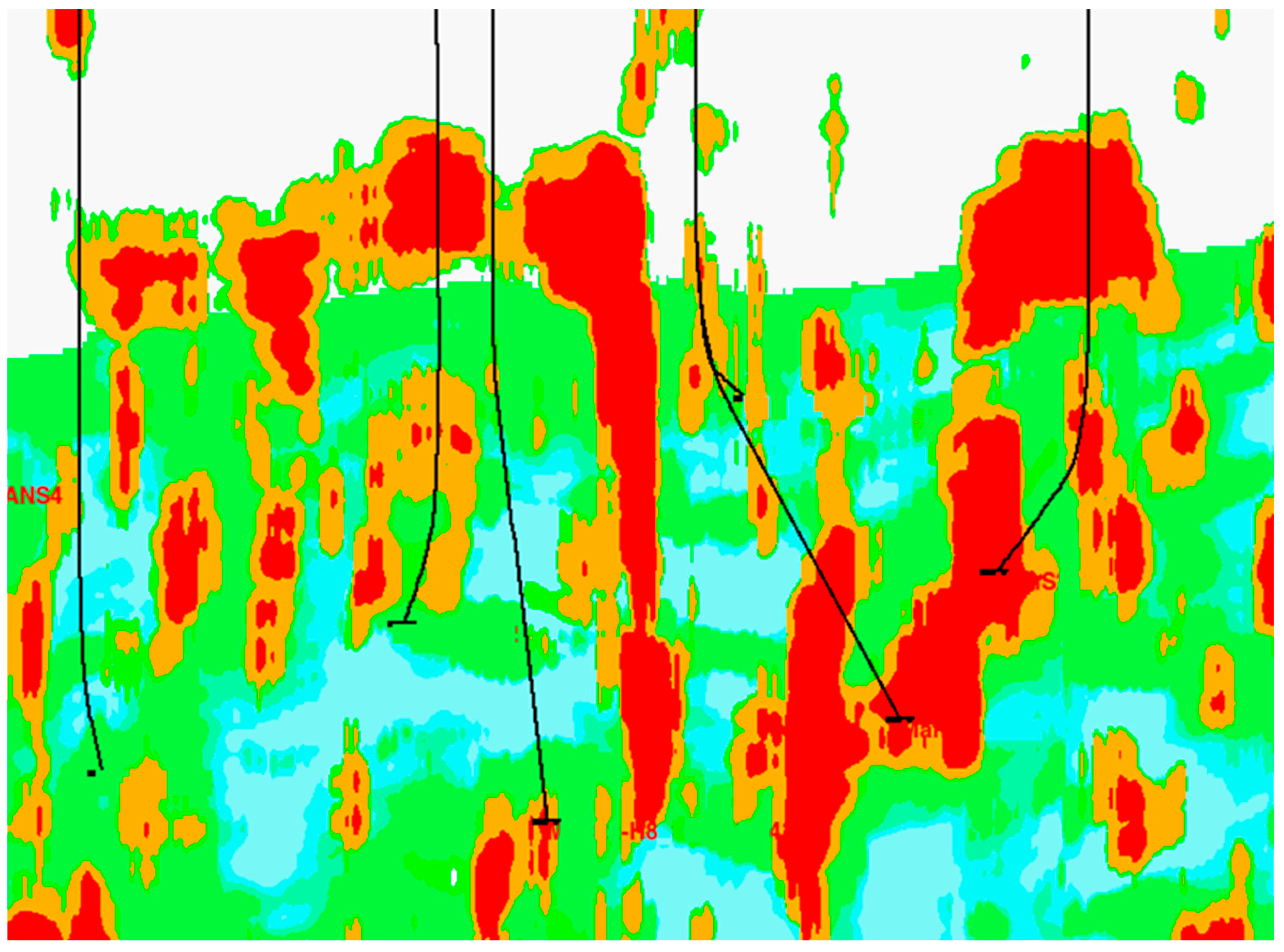
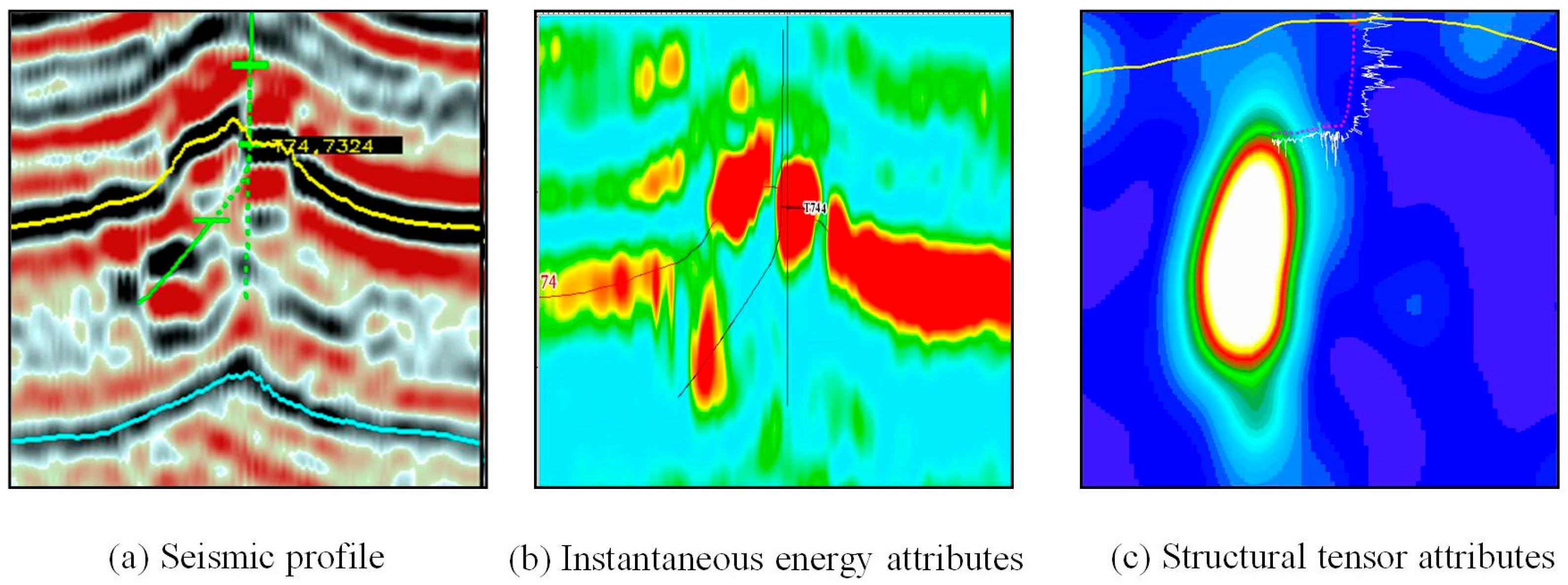
Taking the Xinjiang Oilfield in the Tarim Basin as an example, the geometric shape of its karst caves is extremely irregular, and the fluid flow behavior inside is significantly different from the seepage characteristics of porous media [26]. Figure 1 presents the seismic profile, instantaneous energy attribute and structural tensor attribute diagrams of Xinjiang Oilfield. In this situation, the regular grid system is difficult to accurately depict the morphology of such complex caves. To effectively characterize the cave, the boundary contour of the cave can be approximated by using straight line segments, and the PEBI grid technique can be applied to achieve efficient grid division of fractured caved reservoirs. The principal advantage of the PEBI grid for this specific problem is its local orthogonality and the flexibility of Voronoi tessellation, which allows it to naturally conform to the complex, discontinuous boundaries of the void cave regions, where traditional structured grids would require excessively fine and computationally expensive stair-step approximations. This is critical for preserving the local conservation and solution accuracy around the cave-fracture interface, where pressure exchange is calculated. This grid system is constructed by generating Voronoi polygons (i.e., PEBI grid cells) through Delaunay triangulation. Given that there is no seepage process inside the cave, there is no need to grid the interior of the cave in numerical simulation.

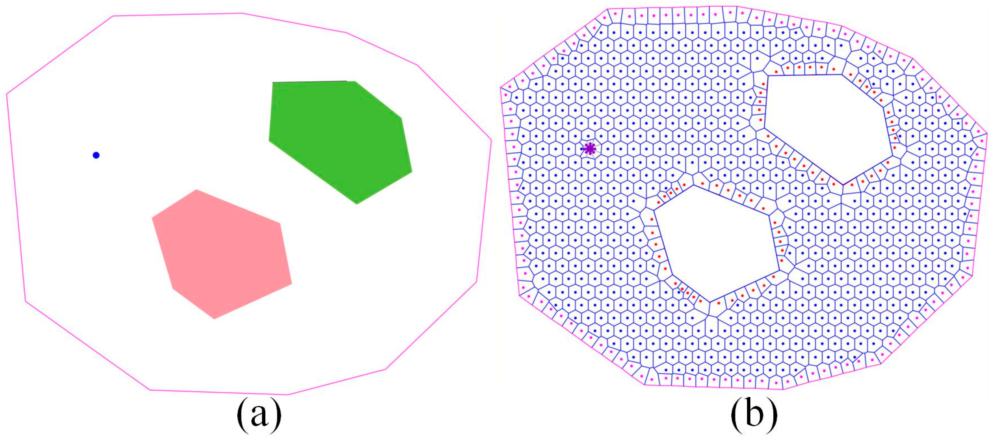
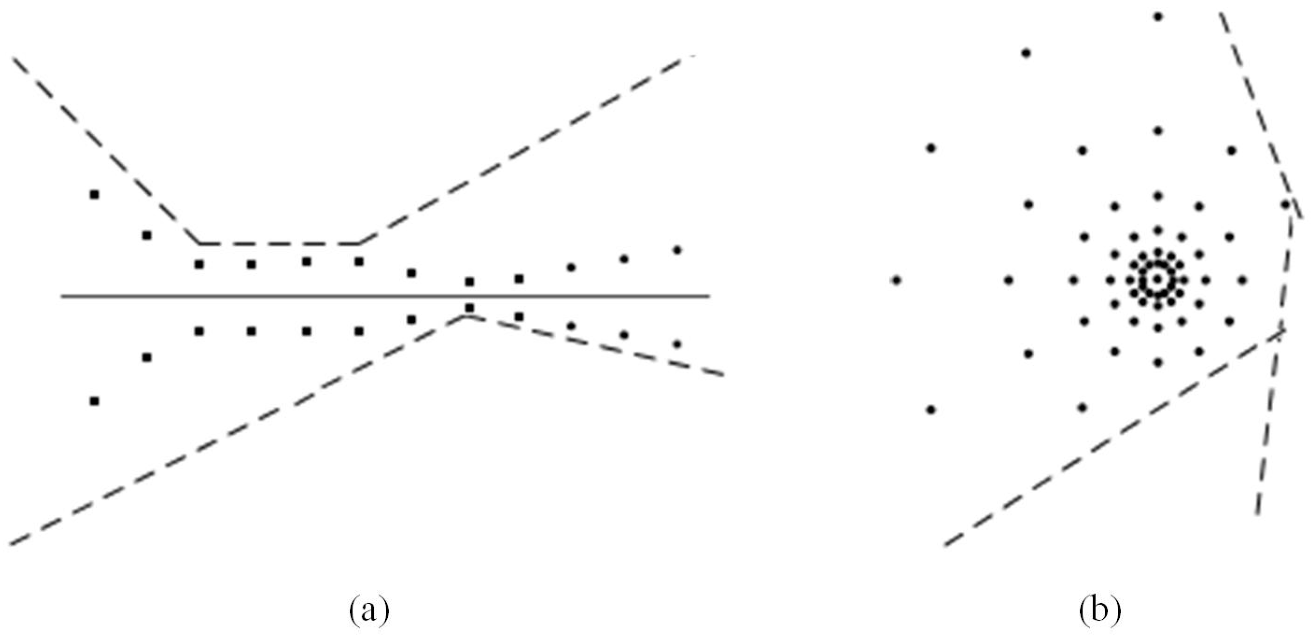
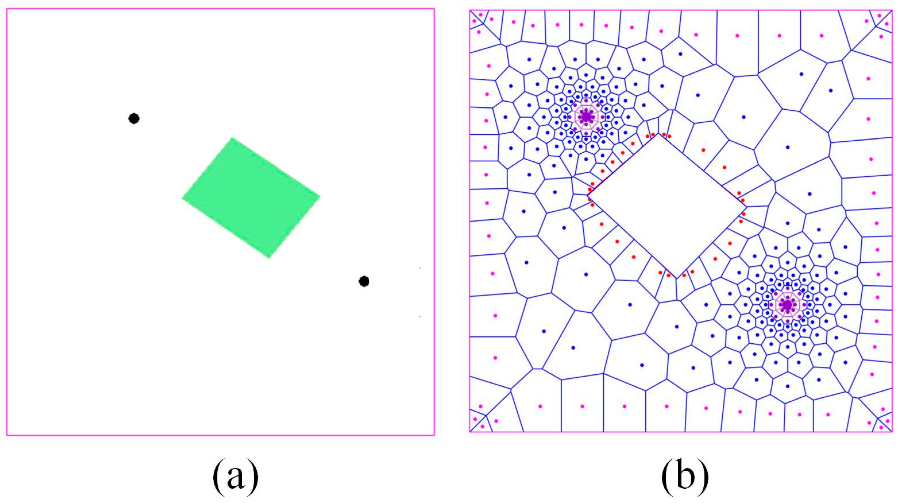
PEBI meshing involves complex geometric calculation processes [27]. In the application of fractured caved reservoirs, since there is no need for grid division inside the cave, the grid lines at its boundaries actually present a discontinuous state (Figure 2), that is, the grid breaks at the cave boundaries. To ensure the accuracy and stability of grid division in fractured caved reservoirs, special grid generation algorithms must be implemented at the karst cave boundaries. Especially when the distance between karst caves and the external boundary of the oil reservoir, between karst caves or between karst caves and the wellbore is too close, grid interference is very likely to occur. Given that both the cave boundary and the oil reservoir boundary are approximated by line segments, and there are different angles between these line segments, and radial flow grids are usually required to be generated near vertical wells, this paper adopts the constraining lines technology (Figure 3) to effectively solve the above grid interference problems.

2.2. Governing Equation

Recent studies innovatively proposed a dynamic flow model for fractured caved reservoirs [28]. By introducing key physical assumptions, the governing equations and definite solution conditions for describing the pressure distribution of such reservoirs were established. Suppose that in carbonate rock strata, apart from discrete karst caves, the fracture network and bedrock jointly form an equivalent porous medium with macroscopic average porosity ϕ and permeability K. When the oil phase is regarded as a slightly compressible single-phase fluid, its seepage behavior follows the following partial differential equation [10]:

$$\nabla \cdot \left[{\displaystyle \frac{K}{\mu B}}(\nabla p-\gamma \nabla Z)\right]={\displaystyle \frac{\mathsf{\partial }}{\mathsf{\partial }t}}\left({\displaystyle \frac{\varphi }{B}}\right)$$

(1)

where K is the permeability of the reservoir matrix; μ is the viscosity of oil; B represents the volume coefficient of the oil phase formation; p is the pressure; γ represents the density of the oil phase; Z represents the vertical coordinate; and ϕ denotes the reservoir matrix porosity.

Unlike conventional porous media, the cave contains no granular matrix. Consequently, pressure changes are not dissipated by slow Darcy-type diffusion through pore throats; instead, they are transmitted purely through the compressibility of the fluid itself, fundamentally in the manner of acoustic or elastic wave propagation. The pressure dynamics inside the cave are therefore governed by the wave equation [24]:

$${\displaystyle \frac{dv}{dt}}+{\displaystyle \frac{1}{\rho C}}{\displaystyle \frac{dp}{dt}}-g=0$$

(2)

where ρ represents the density of the oil; v is the volume expansion rate of the fluid in the cave under isobaric conditions; and g denotes the acceleration due to gravity. C is the propagation speed of the pressure wave and can be calculated by the following formula:

$$C^2={\displaystyle \frac{1}{\rho }}({\displaystyle \frac{1}{M}}+{\displaystyle \frac{1}{\varphi E}})$$

(3)

where M is the bulk modulus of the oil, and E represents the Young’s modulus of the reservoir.

For an infinitesimal pressure drop dp, the fluid undergoes isobaric expansion, producing a relative volume change dv. Being essentially an open volume, the total volumetric change rate inside the cave is simply the net volumetric flow rate entering or leaving the control volume. Neglecting gravitational effects within the cave, integrating Equation (2) over the whole cave volume V immediately yields the lumped-volume form:

$$Q\left(t\right)=-{\displaystyle \frac{V}{\left(1/M+1/\varphi E\right)}}{\displaystyle \frac{d{p}_V}{dt}}$$

(4)

where Q is the flow rate exchanged between the cave and the reservoir; p_V is the variation in pressure in the cave over time. This derivation makes the physical picture clear: the filled-liquid cave behaves as a compressible container whose pressure responds directly to the net accumulation or depletion of fluid, with the responsiveness governed by the wave speed C. The lumped formulation thus provides an intuitive basis for coupling the cave pressure with the fracture-system seepage that controls the net inter-cave flows.

In summary, the classical pure-diffusion model causes the pressure disturbance to attenuate rapidly with distance and time, exhibiting a monotonic and smooth response. In our coupled model, the cave, governed by the wave equation, acts as a dynamic energy capacitor. It absorbs the energy of the incoming diffusion wave, stores it via fluid compression, and then re-releases it, propagating an elastic pressure wave further into the connected fracture network. This dual mechanism has two primary effects: (1) it substantially increases the instantaneous pressure disturbance amplitude observed at the observation well (as energy is channeled and efficiently transmitted), and (2) it introduces a distinct buffer-lag effect, which manifests as the phase lag and the “derivative hump” behavior shown in our sensitivity results. This paragraph is now in Section 2.2, following Equation (4).

2.3. Solution Strategy

Considering the conservation of discrete equations and the use of unstructured PEBI grids, the equations are first integrated as follows:

$${\displaystyle \underset{V_i}{\iiint }\nabla •\left[\frac{K}{\mu B}\left(\nabla p-\gamma \nabla Z\right)\right]d\Omega =}{\displaystyle \underset{V_i}{\iiint }\frac{\mathsf{\partial }}{\mathsf{\partial }t}\left(\frac{\varphi }{B}\right)d\Omega }$$

(5)

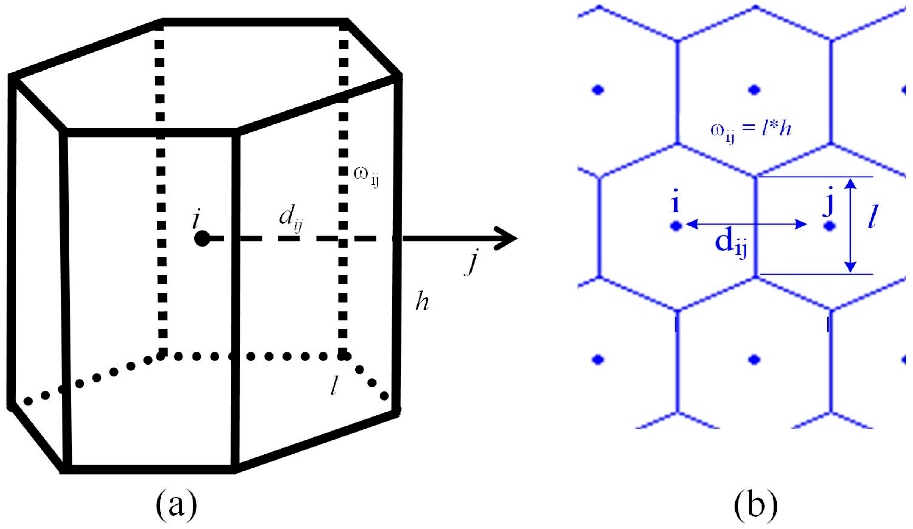
By using the divergence theorem, volume integration is transformed into surface integration. In the PEBI grid shown in Figure 4, the sum of each face in grid i is executed. The left side of Equation (5) can be rewritten as [29]:

$${\displaystyle \underset{S}{∯}\left[\frac{K}{\mu B}(\nabla p-\gamma \nabla Z)\right]}\cdot \overrightarrow{n}ds={\displaystyle \sum _j\left[{\left(\frac{K}{\mu B}\right)}_{ij}\frac{{\omega }_{ij}}{d_{ij}}\left(p_j-p_i-\gamma (Z_j-Z_i)\right)\right]}$$

(6)

The right side of Equation (5) is the cumulative term, which can be discretized as:

$${\displaystyle \underset{V_i}{\iiint }\frac{\mathsf{\partial }}{\mathsf{\partial }t}\left(\frac{\varphi }{B}\right)d\Omega }={\displaystyle \frac{V_i}{\Delta t}}\left[{\left({\displaystyle \frac{\varphi }{B}}\right)}_i^{n+1}-{\left({\displaystyle \frac{\varphi }{B}}\right)}_i^n\right]={\displaystyle \frac{1}{B_i^n}}{\displaystyle \frac{\mathsf{\partial }{\varphi }_i}{\mathsf{\partial }p}}\delta p_i+{\varphi }^{n+1}{\displaystyle \frac{\mathsf{\partial }(1/B_i)}{\mathsf{\partial }p}}\delta p_i$$

(7)

The volume coefficient of porosity and slightly compressible fluid can be approximately given in the following form:

$$\varphi ={\varphi }_{\mathrm{ref}}\left[1+C_r\left(p-p_{\mathrm{ref}}\right)\right]$$

(8)

$$B=B_{\mathrm{ref}}/\left[1+C_f\left(p-p_{\mathrm{ref}}\right)\right]$$

(9)

Combining Equations (6)–(9), we can obtain:

$${\displaystyle \sum _j{T}_{ij}[p_j-p_i-(D_j-D_i)]}={\displaystyle \frac{V_i}{\Delta t}}\left[{\displaystyle \frac{{\varphi }_{\mathrm{ref}}{C}_r}{B^n}}+{\varphi }^{n+1}{\displaystyle \frac{C_f}{B_{ref}}}\right](p_i^{n+1}-p_i^n)$$

(10)

where T represents conductivity; D is the gravity in the grid; p_ref, ϕ_ref and B_ref represent the reference pressure, the porosity and volume coefficient under the reference pressure, respectively. The conductivity of the n + 1 time step can be obtained by Taylor expansion at the previous iteration [30]:

$$T_{ij}^{n+1}\cong T_{ij}^{\begin{array}{l}(v+1)\\ n+1\end{array}}=T_{ij}^{\begin{array}{l}(v)\\ n+1\end{array}}+{\left.{\displaystyle \frac{\mathsf{\partial }{T}_{ij}}{\mathsf{\partial }{p}_i}}\right|}^{\begin{array}{l}(v)\\ n+1\end{array}}\delta p_i^{\begin{array}{l}(v+1)\\ n+1\end{array}}+{\left.{\displaystyle \frac{\mathsf{\partial }{T}_{ij}}{\mathsf{\partial }{p}_j}}\right|}^{\begin{array}{l}(v)\\ n+1\end{array}}\delta p_j^{\begin{array}{l}(v+1)\\ n+1\end{array}}$$

(11)

where the superscripts n and v represent the time step and the iteration step, respectively. The pressure term also takes values in n + 1 time steps:

$$\begin{array}{l}{p}_j^{\begin{array}{l}(v+1)\\ n+1\end{array}}\approx p_j^{\begin{array}{l}(v)\\ n+1\end{array}}+\delta p_j^{\begin{array}{l}(v+1)\\ n+1\end{array}}\\ p_i^{\begin{array}{l}(v+1)\\ n+1\end{array}}\approx p_i^{\begin{array}{l}(v)\\ n+1\end{array}}+\delta p_i^{\begin{array}{l}(v+1)\\ n+1\end{array}}\end{array}$$

(12)

After fully implicit linearization based on spatial upstream weighting, Equation (10) can be expressed as:

$$\begin{array}{l} {\displaystyle \sum _j\left(T_{ij}^{\begin{array}{l}(v)\\ n+1\end{array}}\right)\left(p_j^{\begin{array}{l}(v)\\ n+1\end{array}}-p_i^{\begin{array}{l}(v)\\ n+1\end{array}}-(D_j-D_i)\right)}+{\displaystyle \sum _j\left(T_{ij}^{\begin{array}{l}(v)\\ n+1\end{array}}\right)\left(\delta p_i^{\begin{array}{l}(v+1)\\ n+1\end{array}}-\delta p_i^{\begin{array}{l}(v)\\ n+1\end{array}}\right)}\\ +{\displaystyle \sum _j{\left(\frac{\mathsf{\partial }{T}_{ij}}{\mathsf{\partial }p}\right)}_{+}^{\begin{array}{l}(v)\\ n+1\end{array}}\left(p_j^{\begin{array}{l}(v)\\ n+1\end{array}}-p_i^{\begin{array}{l}(v)\\ n+1\end{array}}-(D_j-D_i)\right)\delta p_{+}^{\begin{array}{l}(v+1)\\ n+1\end{array}}}\\ =C_p^{\begin{array}{l}(v)\\ n+1\end{array}}\delta p_j^{\begin{array}{l}(v+1)\\ n+1\end{array}}+C_p^{\begin{array}{l}(v)\\ n+1\end{array}}(p_i^{\begin{array}{l}(v)\\ n+1\end{array}}-p_i^n)\end{array}$$

(13)

where C_p is the cumulative coefficient, expressed as:

$$C_p={\displaystyle \frac{V_i}{\Delta t}}\left[{\displaystyle \frac{{\varphi }_{\mathrm{ref}}{C}_r}{B^n}}+{\varphi }^{n+1}{\displaystyle \frac{C_f}{B_{ref}}}\right]$$

(14)

We take the cave as a grid with a grid pressure of p_V. The total flow into the grid in all strata connected to the cave is expressed by Darcy’s law. Thus, the cave equation can be discretized as:

$${\displaystyle \sum _j\left[{\left(\frac{K}{\mu B}\right)}_j\frac{{\omega }_j}{d_{Vj}}\left(p_j-p_V\right)\right]=-\frac{V}{\left(1/M+1/\varphi E\right)}\frac{p_V^{n+1}-p_V^n}{\Delta t}}$$

(15)

In pulse well testing, there are active wells and observation wells. If there is no fluid inflow or outflow in the observation well, the flow rate is 0. The active well has the operation of opening and closing the well. The active well can be treated as the inner boundary. Considering the wellbore storage and the skin, it is the bottom hole flow pressure expression of the active well:

$$p_{wf}^{n+1}={\displaystyle \frac{{\displaystyle \sum _j{\left(W{I}_j{\lambda }_j{p}_j\right)}^{n+1}}+\frac{C}{\Delta t}{p}_{wf}^n-Q}{{\displaystyle \sum _j{\left(W{I}_j{\lambda }_j\right)}^{n+1}}+\frac{C}{\Delta t}}}$$

(16)

where WI_j denotes the well index; λ_j represents the pressure function of grid j connected to the well; C refers to the wellbore storage constant; S indicates the epidermal coefficient; p_wf stands for the bottom hole flowing pressure; and Q signifies the flow rate of the injection well.

The characteristic time for an acoustic wave to traverse a karst cave of typical dimensions (tens to hundreds of meters) is on the order of milliseconds, given the pressure wave propagation velocity C (Equation (3), typically ~1450 m/s for water). In contrast, the duration of the pulse well test is on the order of hundreds of hours. Consequently, any internal pressure gradients within the cave equilibrate almost instantaneously relative to the overall test duration. The pressure across the cave volume can thus be considered spatially uniform at the resolution of our simulation timesteps. This does not reduce the model to a simple tank model; rather, the temporal dynamics of this uniform pressure are rigorously derived from the wave equation (Equation (2)). By integrating Equation (2) over the cave volume V and linking the volumetric change rate to the net flow rate Q via the fluid’s compressibility, we arrive at Equation (4). The physical mechanism governing pressure change remains fundamentally the propagation and reflection of elastic pressure waves, which justifies retaining the ‘wave equation’ terminology. The wave velocity C is a direct input parameter controlling the dynamic compressibility and energy buffering capacity of the cave.

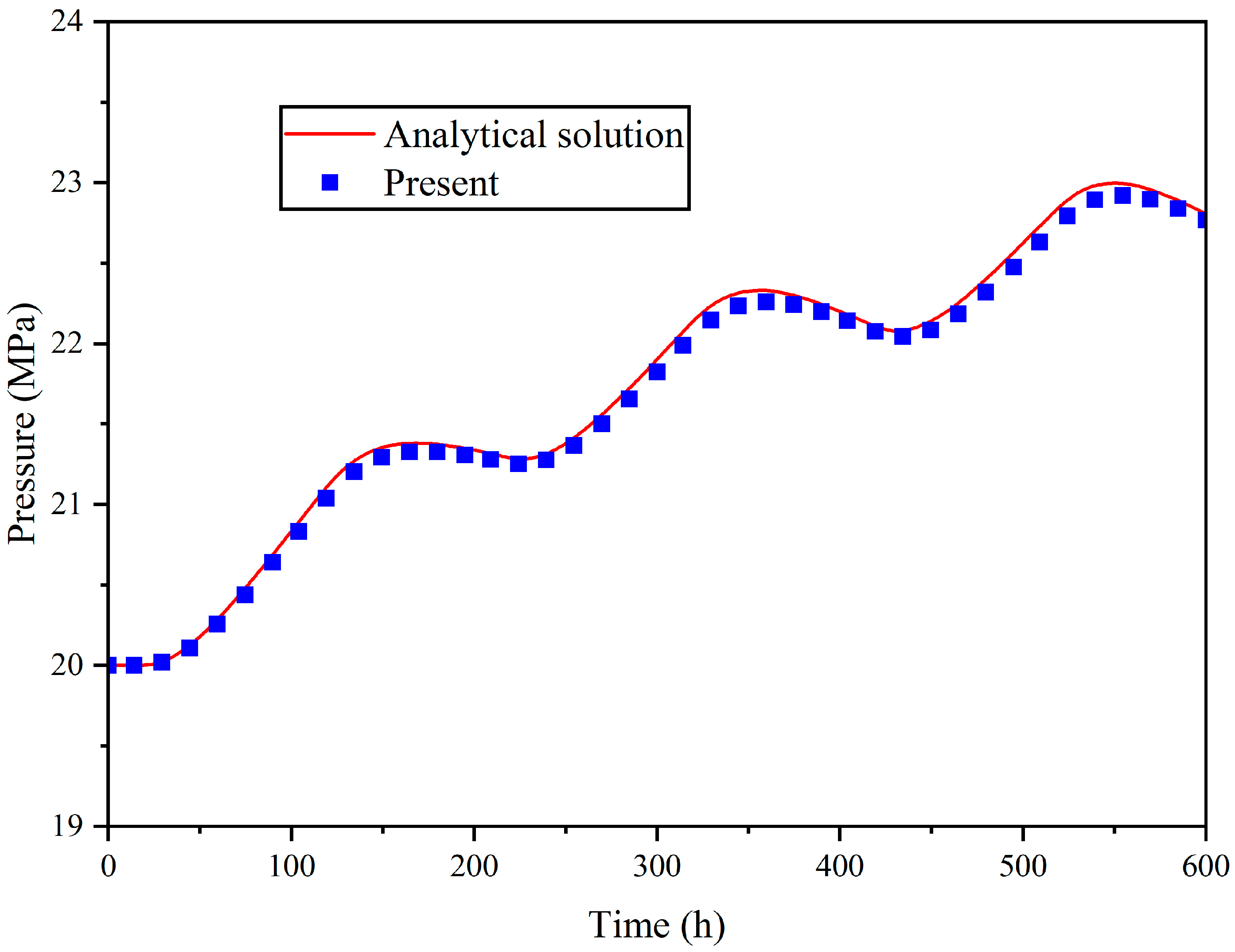
In summary, the overall solution procedure comprises the following steps: (i) spatial discretization of the fracture-matrix system is performed using the unstructured PEBI grid, with the continuum seepage equation integrated by the finite volume method; (ii) the cave is treated as a single computational node whose pressure evolution is governed by the volume-integrated wave equation (Equation (4)); (iii) the exchange flow rate between the cave and the surrounding grid cells is calculated explicitly via Darcy’s law; (iv) the resulting system of nonlinear algebraic equations is linearized fully implicitly and solved iteratively, with the active well handled as an inner boundary condition including wellbore storage and skin.

3. Model Verification

When the volume of the cave is 0, the model degenerates into a simple seepage problem. Considering the wellbore storage constant and the skin in an infinite formation, the expression of the dimensionless pressure at the well with time in the Laplace space analytical solution is [28]:

$${\overline{P}}_D\left(u,t_D\right)={\displaystyle \frac{1}{u}}{\displaystyle \frac{K_0\left(r_D\sqrt{u}\right)}{C_{D}S{K}_0\left(\sqrt{u}\right)+\left(1+C_{D}uS\right)\sqrt{u}{K}_1\left(\sqrt{u}\right)}}$$

(17)

$$C_D={\displaystyle \frac{C}{2\pi r_w^2\varphi h{C}_t}}$$

(18)

$$P_D\left(r_D,t_D\right)={\displaystyle \frac{kh\left[p_i-p\left(r,t\right)\right]}{1.842\times {10}^{-3}QB\mu }}$$

(19)

$$t_D={\displaystyle \frac{3.6kt}{\varphi \mu C_t{r}_w^2}}$$

(20)

$$r_D=r/r_w$$

(21)

$${\overline{P}}_D\left(r_D,u\right)={\displaystyle {\int }_0^{\infty }{P}_D}\left(r_D,t_D\right)e^{-u{t}_D}d{t}_D$$

(22)

where K₀ and K₁ denote the zeroth- and first-order modified Bessel functions of the second kind, respectively. C_D refers to the dimensionless wellbore storage coefficient; P_D(r_D, t_D) stands for dimensionless pressure; t_D indicates dimensionless time; p_i represents the initial formation pressure; p(r, t) denotes the formation pressure distribution; u signifies a Laplace transform variable; r_D is the dimensionless distance between the stimulation well and the observation well.

To verify the reliability of the numerical algorithm proposed in this paper, three-cycle injection and stop pulse excitation were implemented on the active well based on the design parameters in

Table 1. Calculation parameters for well pressure in an infinite formation.

Parameters	Value
The original pressure, pi	20 MPa
Permeability, K	0.001 μm2
Formation thickness, h	10 m
Storage constant, C	0.5 m3/MPa
Radius of the oil well, rw	0.1 m
Skin coefficient, S	0
Porosity, ϕ	0.15
Well distance, L	100 m
Fluid density, ρ	1000 Kg/m3
The side length of the rectangle Xe	10,000 m
Fluid viscosity, μ	1 mPa·s
The side length of the rectangle Ye	10,000 m
Volume coefficient, B	1.1
Injection flow rate, Q	−40 m3/D
Compression coefficient, Ct	0.001 MPa−1
Injection/withdrawal time, t	100 h

. The pressure response of the observed well was obtained by solving Equation (10) through Laplace numerical inversion. Figure 5 shows the dynamic pressure comparison curves of the numerical solution and the classical analytical solution. The results indicate that:

• Consistency of response morphology: The numerical solution fully reproduces the waveform characteristics of the analytical solution, both showing typical pressure lag effects (the response of the observation well is delayed compared to the operation of the active well).
• Pulse period consistency: Both accurately capture three complete pressure pulse periods, and the time sequence of cycle duration and amplitude change is highly consistent with the analytical solution.
• Long-term dynamic deviation: On a large time scale, the numerical solution pressure value is slightly lower than the analytical solution. The maximum deviation occurs at the pulse wave peak position (Δp_max = 0.071 MPa), with an error of 3.55% relative to the original formation pressure, which meets the engineering calculation accuracy requirements. This systematic slight underestimation is mainly attributed to the numerical dispersion inherent in the finite volume discretization and the grid orientation effects of the PEBI mesh, which introduce a marginal additional diffusion compared to the idealized analytical solution. It should be noted that this validation example considers a zero-cave-volume case; it therefore confirms the correctness of the basic seepage solver but does not directly validate the cave wave-equation term. The successful field application presented in Section 5 provides an indirect, yet reasonable, validation of the full model under realistic conditions.

4. Cave Sensitivity Analysis

Based on the above calculation program and parameter values, the pulse pressure of fractured caved reservoirs was calculated. Figure 6 shows the relative positions among the active well, the cave and the observation well. Considering the equal thickness of the stratum, in this paper, the volume of the cave is represented by the area of the cave, and the dimensionless cave area A_D and the dimensionless active well-cave distance L_D are defined. To facilitate the calculation of the cave area, the cave is set as a rectangle, which does not affect the calculation result.

It should be noted that in the sensitivity analysis presented here, the simplification of the cave geometry to a rectangle is solely for the convenience of controlling the area as a single variable. Due to the physical mechanism by which the cave functions primarily as a capacitive volume (Equation (4)), this regularization does not affect the principal conclusions drawn from the sensitivity study. However, for practical field applications involving irregularly shaped caves, the unstructured PEBI grid is an indispensable tool for ensuring geometric fidelity, which is crucial for accurate pressure history matching and parameter inversion.

4.1. Cave Area

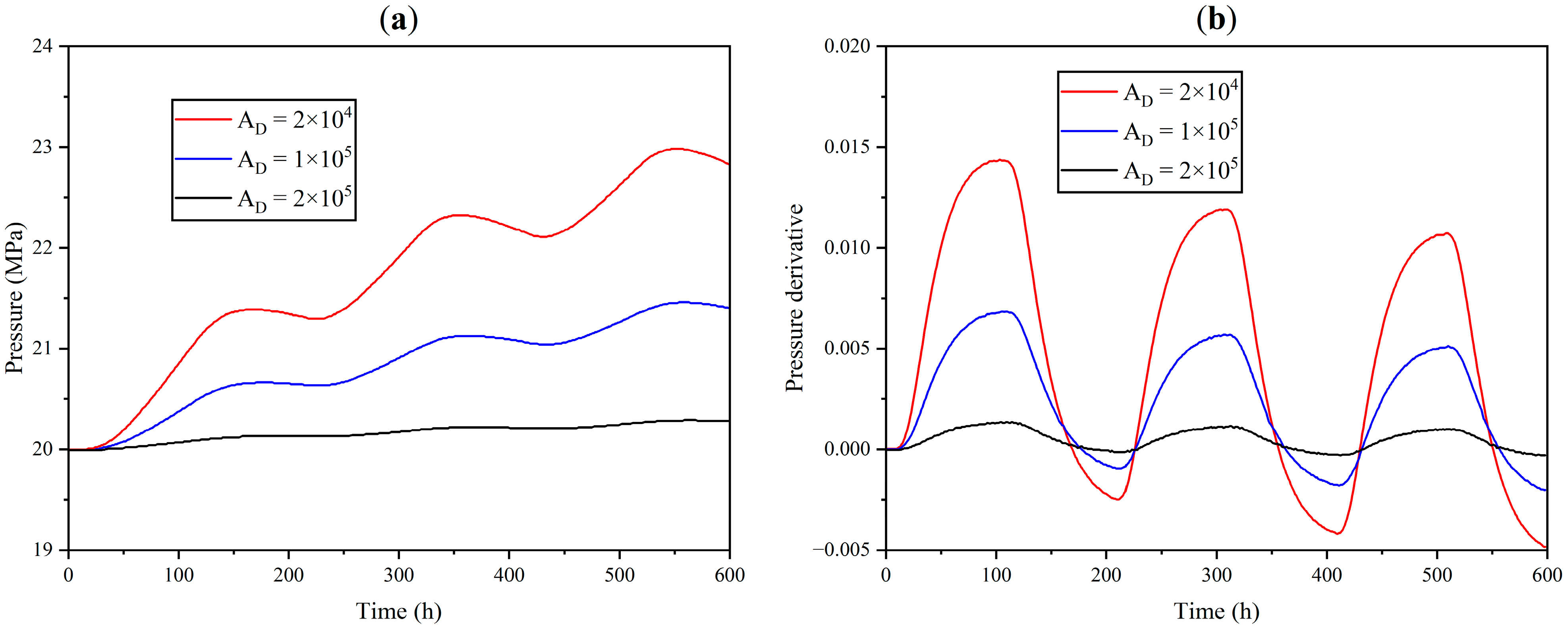
Figure 7 shows the response characteristics of pressure under different cave areas of the observation well and the influence of derivative dynamics on pulse excitation. In the initial stage of injection into the active well (approximately within 24 h), the observation well pressure remains basically unchanged. It then continues to rise until the withdrawal time (100 h). After the injection was stopped, the pressure continued to rise by inertia, reaching a peak about 150 h later and then turning downward. This lag response (phase difference Δt ≈ 50 h) confirms that the operation of the active well has a delayed effect on the observation well through the fracture cave system. The influence of the cave area on the pressure of the observation well. Under the same excitation pressure, the smaller the cave area, the greater the variation range of the observation well pressure. When observing the maximum pressure of the well, when observing the maximum pressure of the well. The larger the volume of the cave, the smaller the pressure variation in the observation well (Figure 7a), and the smaller the distance between the maximum and minimum values of the pressure derivative (Figure 7b). Under the same excitation pressure, the size of the cave area has no effect on the time for observing the pressure change in the well. As the pulse period increases, the minimum value of the derivative shifts downward, and stopping the injection leads to an increase in the pressure drop of the observation well. These phenomena can be explained by the fact that the pressure change in the fluid in the cave is a wave propagation. When the pressure changes in the active well diffuse to the cave through seepage, the compressive characteristics of the fluid inside the cave enable the karst cave to play a role in energy storage and buffering against the pressure changes. After buffering, the pressure changes diffuse to the observation well through seepage. A larger cave volume corresponds to a greater fluid mass and a larger effective capacitance (ρCqV). During the injection pulse, a larger cavity absorbs more energy to achieve the same pressure increase, thereby attenuating the pressure amplitude transmitted to the observation well and smoothing the pressure derivative response.

4.2. Cave-Well Distances

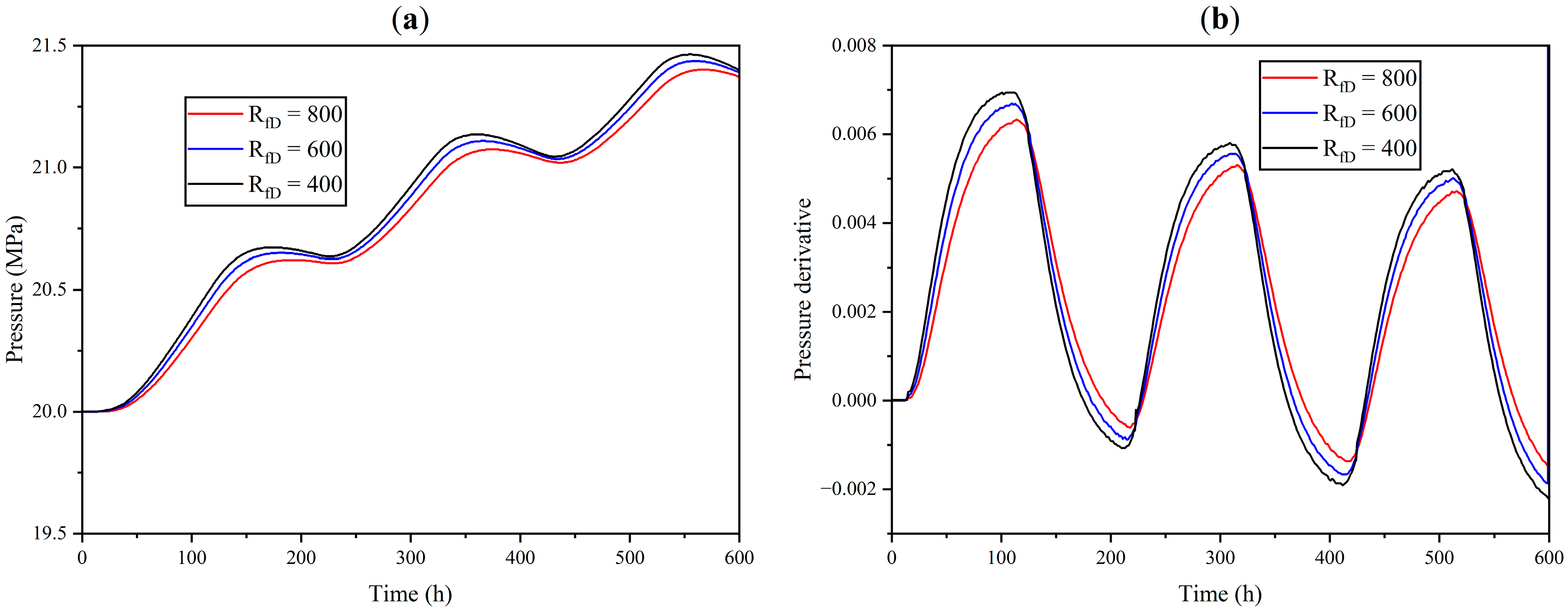
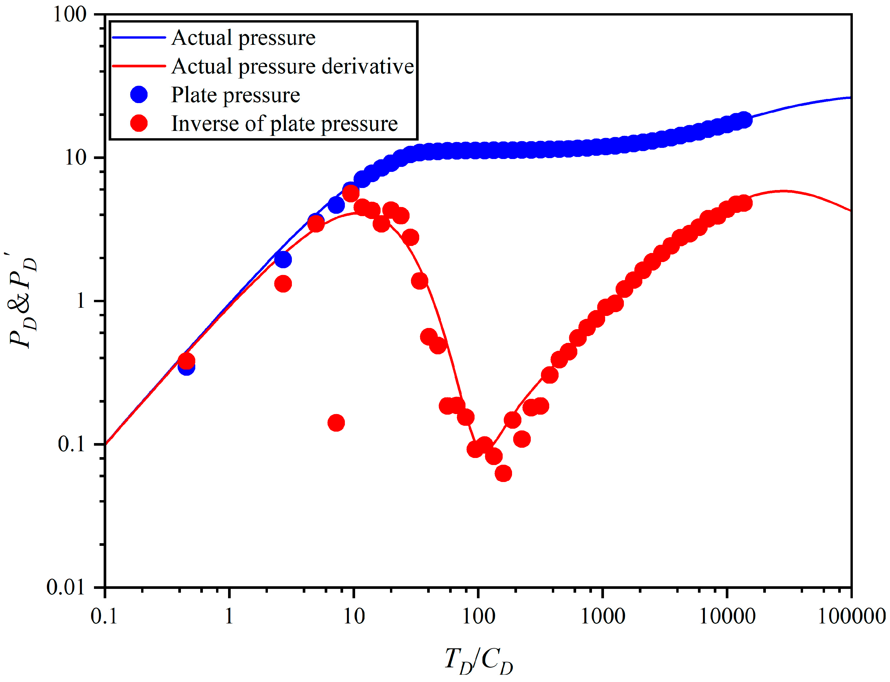
Subsequently, we studied the influence of the cave location on pressure and pressure derivatives. Figure 8 presents the double logarithmic curves of the pressure and the derivative of the observation well at different cave-well distances. It can be seen that the shorter the distance between the cave and the active well, the greater the pressure disturbance amplitude of the observation well. Conversely, the farther the distance, the later the peak of the pressure derivative appears, but the difference is not significant. For instance, when the dimensionless distance LD was increased from 400 to 800, the peak-to-peak pressure variation amplitude at the observation well decreased by only ap-proximately 0.28%, which quantifiably confirms the relatively limited sensitivity compared to a three-fold change in cave volume.

The above-mentioned law can be reasonably explained by the analytical solution of point source seepage in an infinitely large stratum. In the area between the active well and the karst cave, the pressure propagation satisfies the diffusion equation. The well can be regarded as an instantaneous point source, and the pressure response at any point in the formation can be expressed as:

$$p\left(r,t\right)=p_i+{\displaystyle \frac{1}{2}}{\displaystyle \frac{kh}{1.842\times {10}^{-3}QB\mu }}{E}_i\left(-{\displaystyle \frac{r^2\varphi \mu C_t}{14.4kt}}\right)$$

(23)

where the exponential integral can be expressed as:

$$-E_i\left(-x\right)={\displaystyle {\int }_x^{\infty }\frac{e^{-u}}{u}du}$$

(24)

To directly link this analytical solution to the numerical results, let the shortest distance from the active well to the cave boundary be L. By replacing r in Equation (23) with L, the disturbance caused by the flow rate of the active well to the pressure inside the cave can be quantified. This analytical relationship reproduces two key numerical observations:

First, because the exponential integral function is monotonically decreasing, the larger L is, the smaller the pressure calculated by Equation (23) will be—meaning that the pressure disturbance of the active well on the cave becomes weaker, and the pressure variation range recorded by the observation well decreases accordingly. Second, constrained by the slowly varying nature of the exponential integral function, even when L changes considerably, the corresponding pressure change remains relatively modest. This explains why, in the numerical simulations, the distance between the cave and the well affects the pressure response of the observation well, but the overall variation range is limited, matching the behavior predicted by the analytical solution.

4.3. Active Well Flow Rate

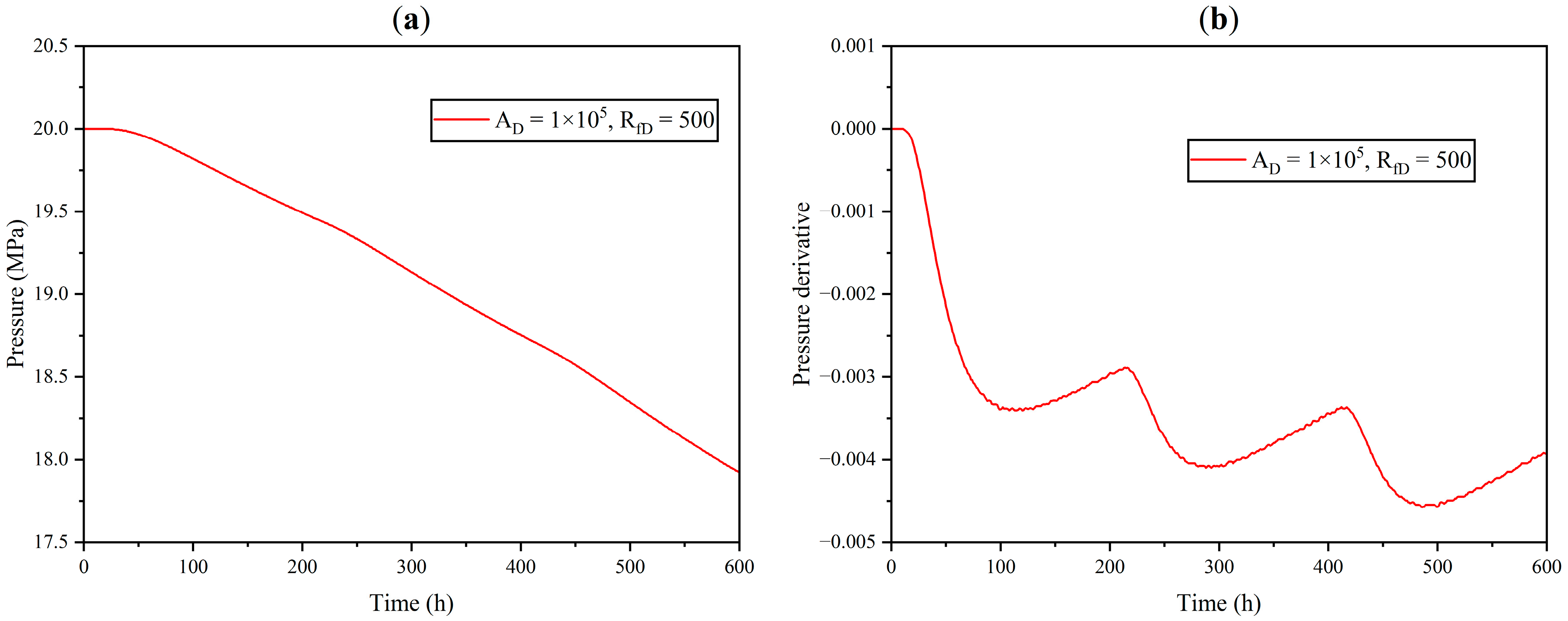
For the standard process of disturbance/impulse well testing in fractured caved reservoirs, we implement stepwise production variations in the active wells and record the pressure responses in the observation wells. We set A_D = 1 × 10⁵ and R_fD = 500. Then, when t is between 0 and 200, 200 and 400, and 400 and 600, the active well flow rates are 100, 200 and 300, respectively. Figure 9 shows the variation in observation well pressure with time in fractured caved reservoirs under variable production. It can be seen from Figure 9a that the pressure in the observation well varies with time. When the flow is stable, the pressure has an approximately linear relationship with time. The slope of the well pressure varies when the flow rate is different. The time when the slope changes is different from the time when the flow rate changes, and a lag phenomenon occurs in the slope change in the observation well. Figure 9b shows the variation in the pressure derivative of the observation well with time under variable production in fractured and cave-shaped oil reservoirs. It can be seen from the figure that the derivative is generally negative, indicating that the pressure is generally decreasing. The derivative shows the characteristic of fluctuating changes, and the derivative feature is more obvious compared with the pressure. However, the derivative value is very small. In actual measurement, the accuracy error of the pressure gauge and environmental noise may mask the change in the pressure derivative. In actual field measurements, the accuracy limitations of pressure gauges and environmental noise can easily mask these subtle pressure derivative changes. This severely limits the practical applicability of pressure derivative interpretation in such reservoirs.

5. Field Application

5.1. Pressure Buildup Test Interpretation for Well Xinjiang-1H

The primary fluid storage space in fractured-vuggy reservoirs is composed of caves. Although the initial oil production rate from these caves can be high, reservoir pressure declines rapidly. Consequently, water injection is required to elevate the reservoir pressure, with injection from adjacent wells being one of the viable strategies. Water flooding production via neighboring wells necessitates an understanding of inter-well connectivity, for which pulse testing serves as a key diagnostic technique.

To illustrate the application of this methodology, wells Xinjiang-1H and Xinjiang-2H were selected. Figure 10 presents the well location map of Xinjiang-1H and Xinjiang-2H, along with the cave distribution interpreted from seismic data (caves are indicated in red). Based on seismic interpretation, the volume of the cavernous region between Xinjiang-1H and Xinjiang-2H is 88,000 m³.

A five-day pressure buildup test was conducted on well Xinjiang-1H on 16 April 2019. Prior to the shut-in period, the production rate was relatively stable, with an average daily oil rate of 136 t/D. For comparison with the pulse-test interpretation results, the well-test interpretation results for Xinjiang-1H from 16 April 2019 are presented herein. Figure 11 shows the log-log type-curve matching plot of pressure and pressure derivative for well Xinjiang-1H. Using the basic parameters provided in

Table 2. Basic parameters of formation and fluid in active wells and observation wells.

Parameters	Value
The thickness of the stratum, h	10 m
Radius of the oil well, Rw	0.6236 m
Porosity, ϕ	0.15
Fluid viscosity, μ	0.58 mPa·s
Volume coefficient, B	1.1
The compression coefficient, Ct	0.001 MPa−1
The depth in the middle H1	6700 m
Fluid density, ρ	860 Kg/m3
Fluid compression coefficient, Cq	0.00085 MPa−1

, the well-test interpretation yields a permeability of 86.3 × 10⁻³ μm², a kh/μ value of 3260 × 10⁻³ μm²·m/(mPa·s), a cave distance of 238.7 m from well Xinjiang-1H, a cave volume of 52,000 m³, and an investigation radius of 471 m.

5.2. Interference Well Testing for Inter-Well Connectivity

To test the inter-well connectivity of Xinjiang Oilfield, interference well testing operations were carried out from 5 to 22 July 2019. Among them, well Xinjiang1-1H was used as an observation well and well Xinjiang1-20H was used as an active well. The measured bottomhole pressures at the observation well during each flow rate step were 129.0 MPa, 128.6 MPa, 128.0 MPa, and 127.9 MPa, respectively, with corresponding pressure drop rates of 0.00072, 0.00129, 0.00173, and 0.00187 MPa/h. The well test process is shown in

Table 3. Well test process.

Active Wellhead Action	Active Well		Observation Well
Increase from 5 to 5.5	6 July 2019 12:55	82.8	9 July 2019 4:45	129
Increase from 5.5 to 6	11 July 2019 18:00	95.3	15 July 2019 10:50	128.6
Increase from 6 to 6.5	15 July 2019 17:17	112.6	19 July 2019 0:30	128
	11 July 2019 18:00	125.9	20 July 2019 15:50	127.9

. Table 2 presents the basic formation and fluid parameters of the active well and the observation well.

Figure 12 presents the curve of the bottom hole flow pressure of observation well Xinjiang1-1H varying with time. During the interference test period, the overall flow pressure of this well showed a continuous and slight downward trend. When the working cycle of the active well Xinjiang1-20H was successively increased from 5 mm to 5.5 mm, 6 mm and 6.5 mm, the bottom hole pressure of Xinjiang1-1H showed three obvious stepwise fluctuations, and the pressure drop rate increased step by step. They are 0.00072, 0.00129, 0.00173 and 0.00187 MPa/h, respectively. Based on this, it can be determined that there is an effective connection between wells Xinjiang1-20H and Xinjiang1-1H. Taking the corresponding moments of each pressure drop turning point as the landmark time points for the arrival of pressure waves in adjacent wells, the pressure propagation velocity is calculated to be between 18.9 and 42.1 m/h.

The excitation time of production variation in Table 2 and the basic parameters in Table 3, with the distance between the observation well and the active well being 1676.28, were simulated and calculated using a 4000 m × 1600 m rectangular reservoir. By adjusting the relevant parameters, the curve fitting of the observation well was achieved in Figure 10. The parameters input during the fitting are shown in

Table 4. Observe the parameters obtained from the curve fitting of the well.

Parameters	Value
Flow coefficient, kh/μ	2840 × 10−3 μm2·m/(mPa·s)
Storage capacity coefficient, ϕCth	9.31 × 10−4 m/MPa
The volume of the cave, V	67,000 m3
The distance between the cave and the observation well, L	190 m

. Compared with independent seismic attributes that indicate a cave volume of ~62,000 m³ and a cave-to-observation-well distance of ~210 m within the same reservoir interval, the inverted values (67,000 m³ and 190 m) deviate by 8% and 9.5%, respectively, supporting the overall consistency of the interpretation. Nevertheless, the inversion is non-unique; alternative parameter combinations (e.g., cave volume 50,000–80,000 m³ and distance 150–230 m) can produce pressure matches within the measurement error of ±0.2 MPa, and uncertainty propagation from ±10% variations in porosity or total compressibility leads to approximately ±15% range in the inferred cave volume.

5.3. Discussion on Cave Volume Discrepancy

The cave volume obtained from seismic interpretation in this study is larger for two main reasons. First, conventional three-dimensional seismic data have a resolution of 10–30 m, while low-frequency deep seismic data have an even coarser resolution of 50–100 m. The mid-depth of the producing zone in this well is 6700 m; the low seismic resolution, therefore, introduces significant error into the cave-volume estimate. Second, some caves between Xinjiang-1H and Xinjiang-2H indicated by the seismic data may be disconnected and thus do not participate in fluid flow. The well test yields the smallest cave volume because it was conducted solely on Xinjiang-1H; the investigation radius is 471 m, which is considerably smaller than the inter-well distance. Consequently, all interpreted parameters represent average values within a 471 m radius, leading to the minimal cave volume from the well test. The kh/μ value from the well test is 3260 × 10⁻³ μm²·m/(mPa·s), which is in close agreement with the pulse-test result, although the well-test value is slightly higher than that derived from the interference test.

6. Conclusions

This paper studies the pulse well testing of fractured caved reservoirs by using the unstructured PEBI grid numerical simulation method. Through the simulation calculation of the “active well–karst cave–observation well” system, the following conclusions are drawn:

• Unstructured PEBI grids can precisely characterize the boundaries of caves and are a relatively accurate method in numerical simulation of fractured caved reservoirs. This method is applied to simulate the “active well–karst cave–observation well” system, and the variation curve of the observation well pressure with time is obtained, which can be used for the study of pulse well testing in fractured caved reservoirs.
• The volume of the karst cave is a key parameter that affects the pressure and pressure derivative changes in the observation well. The larger the volume of the cave, the smaller the pressure variation range of the observation well, and the gentler the pressure derivative change.
• The distance between the active well and the karst cave also significantly affects the pressure response of the observation well. The greater the distance, the smaller the variation range of the pressure in the observation well, and at the same time, the occurrence time of the peak value of its pressure derivative is delayed.
• The numerical simulation algorithm based on unstructured PEBI grids can effectively history-match the observed pressure transients from observation wells during pulse testing, thereby enabling the interpretation of pulse test data in fractured–caved reservoirs. Key parameters such as cave volume and location can be obtained. To reduce the non-uniqueness of the interpretation, the pressure-derivative history of the observation well can be additionally matched. It should be noted, however, that the derivative curve in this case takes both positive and negative values and exhibits complex fluctuating shapes due to the superposition of periodic pulse excitations and the buffering effect of the cave. This complexity makes semi-log or log-log derivative matching challenging. Therefore, direct history matching in Cartesian coordinates—fitting both pressure and pressure derivative simultaneously—provides a more practical and visually demonstrable approach for parameter estimation in such scenarios, rather than relying on conventional log-log derivative matching.
• This method was applied to the curve fitting of interference well test data in the Xinjiang area, and the results were basically consistent with the interpretation results of pressure recovery data.